A Novel AI Framework for PM Pollution Prediction Applied to a Greek Port City

Abstract

Particulate matter (PM) pollution is a major global concern due to its negative impact on human health. To effectively address this issue, it is crucial to have a reliable and efficient forecasting system. In this study, we propose a framework for predicting particulate matter concentrations by utilizing publicly available data from low-cost sensors and deep learning. We model the temporal variability through a novel Long Short-Term Memory Neural Network that offers a level of interpretability. The spatial dependence of particulate matter pollution in urban areas is modeled by incorporating characteristics of the urban agglomeration, namely, mean population density and mean floor area ratio. Our approach is general and scalable, as it can be applied to any type of sensor. Moreover, our framework allows for portable sensors, either mounted on vehicles or used by people. We demonstrate its effectiveness through a case study in Greece, where dense urban environments combined with low cost sensor networks is a peculiarity. Specifically, we consider Patras, a Greek port city, where the net PM pollution comes from a variety of sources, including traffic, port activity and domestic heating. Our model achieves a forecasting accuracy comparable to the resolution of the sensors and provides meaningful insights into the results.

1. Introduction

Particulate matter (PM) pollution poses a substantial global health threat, as emphasized by the World Health Organization [1]. This type of pollution adversely impacts the functionality of both cardiovascular and respiratory systems. Among the most detrimental to human health [2] are ${\mathrm{PM}}_{1.0}$, ${\mathrm{PM}}_{2.5}$ and ${\mathrm{PM}}_{10}$ particles, with aerodynamic diameters less than 1 $\mathsf{\mu }$m, 2.5 $\mathsf{\mu }$m and 10 $\mathsf{\mu }$m, respectively [3]. Notably, PM pollution has been correlated with COVID-19 infection dynamics [4,5,6], while the aforementioned types of PM are also associated with a heightened risk of cancer [7,8].

The most abundant natural $\mathrm{PM}$ particles are sea salt originating from the Earth’s oceans, mineral dust originating from arid and semi-arid areas and volcanic and biogenic emissions [9]. Anthropogenic particles are produced from industrial complexes (e.g., petrochemical plants, coal-powered power stations), transportation (vehicle/shipping emissions), residential heating [10], biomass burning [11] and more. These particles may be transported long distances from their source (>1000 km) by mesoscale and synoptic circulations, depending on their aerodynamic properties and chemical reactivity [12]. The turbulent condition of the Planetary Boundary Layer (PBL) plays a significant role in determining $\mathrm{PM}$ concentrations within the lower layers of the troposphere as well [13]. $\mathrm{PM}$ particles influence the energy budget of the atmosphere by scattering and absorbing solar radiation and by absorbing and (re)emitting infrared radiation. Some of these particles interact with water vapor and other hydrometeors in clouds, thus influencing cloud dynamics and precipitation characteristics such as the total amount produced and the maximum rates [12].

A specific case of the general picture which is of particular interest is the distribution of PM concentrations in dense urban environments. In these environments, as scale-dependent phenomena emerge (e.g., street canyons effects) along with high aerodynamic roughness of the built area, the complexity of the flow increases greatly, thus affecting PM dispersion. Circulations can also be induced by localized steep temperature gradients [14]. As human-induced emissions show a significant spatiotemporal variation and are heavily influenced by meteorological conditions such as wind speed and relative humidity, which are also extremely time-dependent, modeling and forecasting PM pollution in urban environments presents a substantial challenge.

There are two main approaches to forecasting PM pollution, namely, transport models (for example CALPUFF [15], ADMS-5 [16,17], CAMx [18]) and Computational Fluid Dynamics (CFD) [19,20,21] approaches. In general, transport models allow for somewhat coarse modeling of large spatial scales, from 100 m (ADMS-5) to a whole hemi-sphere (CAMx), while CFD models allow for very detailed modeling, though focused on small scales. It is shown in [15] that dispersion models (e.g., [22]) are less accurate within the complex agglomeration of a city; thus, a prominent approach would be to employ a CFD framework in such environments. However, this task could be very costly in terms of computational resources and, for some applications, practically impossible. For instance, Ref. [15] studied an area of about 1.2 km${}^2$, which is much smaller than the area of a medium-sized city, which could be of the order of 10 km${}^2$. Moreover, an ever-present difficulty in both the aforementioned approaches is the need for detailed modeling of the pollution sources to be used as input to the simulation [23]. Another difficulty is that the resulting modeling framework cannot be generalized easily, as each city has its own time-dependent emissions budget. A way to overcome the above difficulties is to use a purely model-agnostic approach, i.e., Artificial Intelligence (AI) and, specifically, Artificial Neural Networks (ANNs).

Applications of AI towards predicting PM concentrations can be found in the literature, with the first work of this kind published almost two decades ago [24]. Over last few years, the community has been actively exploring Deep Learning approaches to PM prediction, with very good results [25,26,27,28,29,30,31,32,33,34,35,36,37,38,39,40,41,42]. Despite the accurate predictions of ANNs, and the fact that they often outperform classical machine learning algorithms, they receive criticism for being “black boxes” [43]. In order to maintain the high predictability while also ensuring meaningful insight into the results, there are approaches offering a level of interpretability on the final prediction outcome. A recent work [44] constructs a novel kind of Long Short-Term Memory (LSTM) ANN network that allows for both high-quality predictions and interpretations of the final result.

In parallel, the availability of low-cost sensors in the market drives both citizen science initiatives and public authorities [45] towards the creation of low-cost sensor networks for air quality monitoring. Moreover, there are also citizen science initiatives that do not rely on commercial sensors, e.g., [46] allowing for enhanced accessibility to ambient air quality assessments. In addition, low-cost sensors are designed to function autonomously, enabling non-expert users to engage in air pollution monitoring without requiring specialized technical knowledge regarding data acquisition, processing and transmission. Indeed, such networks have been operating in many cities around the globe (e.g., [47]) for the last few years, resulting in accumulated open datasets.

In the current work, we leverage the novel LSTM networks introduced by [44] to enhance the interpretability of our PM concentration predictions. Our research endeavors are aimed towards a cost-efficient prediction framework. A fundamental aspect of our approach involves the integration of openly available data from low-cost sensors, as, for example, in [48,49]. Furthermore, we delineate a set of novel features capable of accurately quantifying the spatial dependencies inherent in urban PM pollution which arise from both urban structures and local PM emissions.

The structure of this paper is organized as follows: Section 2 elucidates the methodology and datasets employed in our analysis; Section 3 presents and deliberates upon our findings; lastly, Section 4 encapsulates our conclusions.

2. Data and Methodology

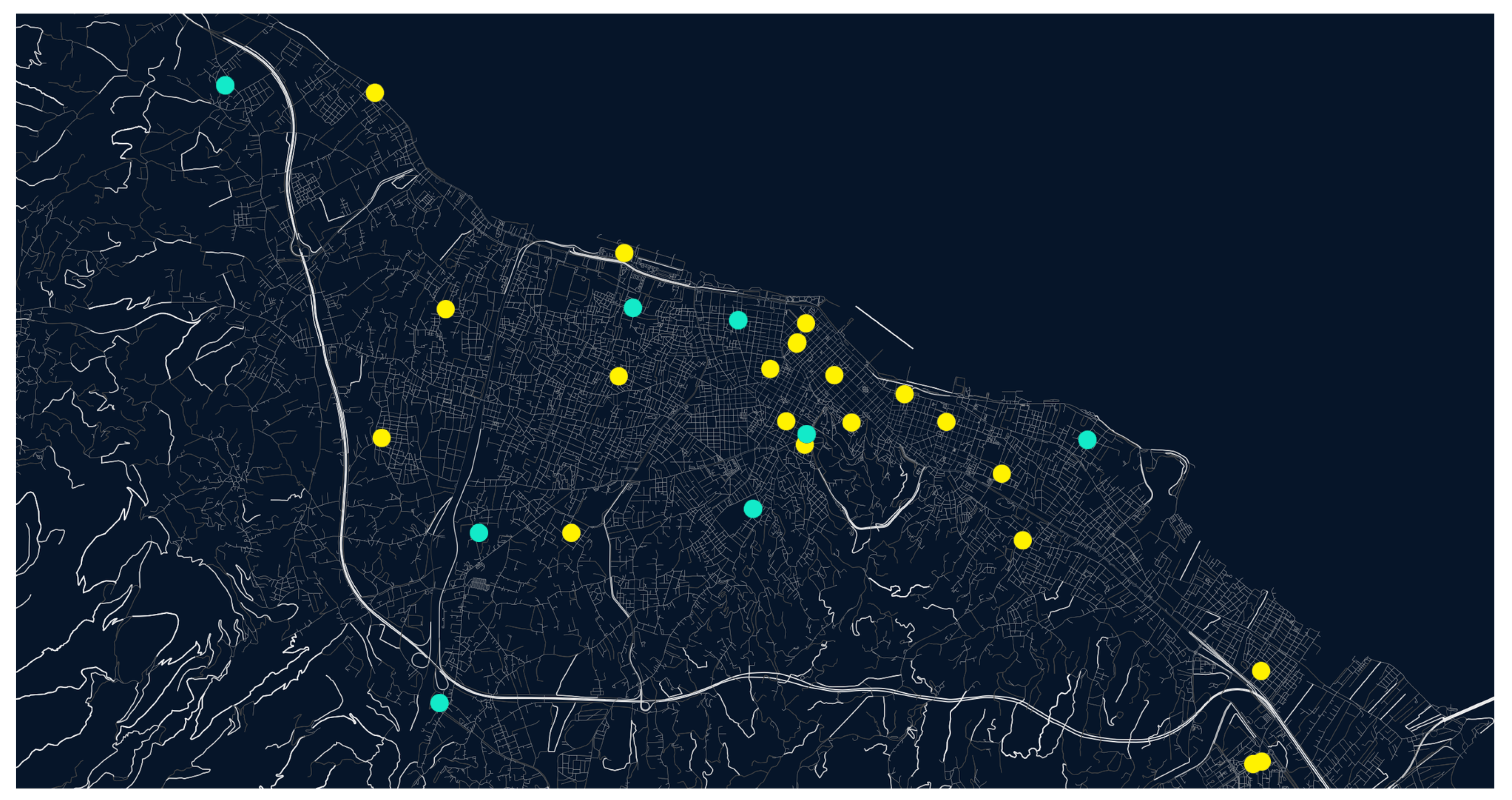
The framework developed for our analysis, outlined in this section, is capable of accommodating any type of observable PM or gas pollutant. It is also sensor-agnostic, in the sense that it is applicable to any sensor type, provided that sensor-specific calibration procedures are integrated into data pre-processing. Furthermore, one may use as additional features specific properties of a PM sensor’s sub-net, such as its resolution. Our approach allows for easy sensor addition or removal and can incorporate portable sensor, for instance, using drones [50] or city buses [51]. These characteristics underline the framework’s flexibility as public sensors can be seamlessly integrated, in alignment with the principles of citizen science. While our methodology is applicable to any urban area, accounting for its unique characteristics, we have chosen the greater area of Patras as a case study to demonstrate the implementation and effectiveness of our framework in a real-world complex urban setting.

2.1. Area of Study

The greater Patras area (city center and suburbs) is located in the northwestern Peloponnese (38${}^{\circ }$14′ N, 21${}^{\circ }$4′ E), approximately 220 km west of Athens. This region is characterized by a hot-summer Mediterranean climate (Csa, Köppen–Geiger climate classification), with daily average temperatures ranging from 6.1 ${}^{\circ }$C in January to 25.3 ${}^{\circ }$C in August. The wettest month is November, with an average accumulated precipitation of 118${}^{\circ }$, while July is the driest, with 4.2 mm [52]. Investigating air quality in Patras carries substantial scientific interest, as it is the third largest city in Greece, housing over 200,000 residents. There are many sources of PM pollution with comparable contributions to total PM loading, all characterized by notable spatiotemporal variations [49]. The southern part of the city features an international port, particularly active during the summer season. It primarily serves passenger ships rather than cargo vessels; however, along the same lines of [53], we suspect that contribution to PM loading during the high season is probable. A small industrial zone is situated 16 km southwest of the city center, hosting several light industries, including pharmaceuticals, food and beverages. North and southwest of the city, there are also popular tourist resorts that draw the attention of many people during the summer period.

The contribution of biomass burning, such as agricultural waste (olive tree branches), from rural areas surrounding Patras is estimated to be up to 7% for ${\mathrm{PM}}_{2.5}$ and 10% for ${\mathrm{PM}}_{10}$ [54]. Studies suggest that during days with high pollution, this contribution can reach up to 50% due to low mixing [11]. Anthropogenic PM particles in Patras mainly consist of organic aerosols (OA) and sulfates. The main sources of OA are very oxygenated OA (V-OOA), moderately oxygenated OA (M-OOA), biogenic oxygenated OA (b-OOA), hydrocarbon-like OA (HOA-1), which related to traffic sources, and hydrocarbon-like OA (HOA-2) from other primary emissions (including cooking) [55]. The most prevalent source of anthropogenic ${\mathrm{PM}}_{10}$ particles is traffic (46.2%) [56], while natural ${\mathrm{PM}}_{10}$ particles observed over Patras are primarily due to the long-range transport of Saharan dust. Extreme cases of dust transport over Greece are frequent throughout the year [57]. As far as ${\mathrm{PM}}_{2.5}$ contributors are concerned, a 2011 study identified secondary sulfate (34%), traffic emissions (34%), biomass burning (11%), shipping (10%), sea salt (11%) and mineral dust (2%) as the major sources in the city center, and secondary sulfate (34%), traffic emissions (25%), biomass burning (15%), mineral dust (10%) and sea salt (5%) as the major sources in a suburban site in Patras [58]. Biomass burning for residential heating is the most important organic aerosol source in the area during winter [59].

Air quality over Patras is determined by the stability of the Planetary Boundary Layer (PBL) and its turbulent state. During unstable conditions, particulate matter may be diluted via vertical mixing within the PBL, which often reaches 2 km above ground level. This is a common case during daytime, with low cloud cover and moderate winds. On the other hand, the atmosphere is more stable during night-time, so pollution cannot be mixed at higher altitudes. Local air flows, such as sea breezes or mountain–valley winds, also affect the air quality of Patras. Additionally, the complex topography of this region modifies the wind patterns by trapping pollutants in certain areas or causing pollutant plumes to disperse unevenly. All the aforementioned factors pose an additional challenge for assessing and forecasting air quality with high confidence.

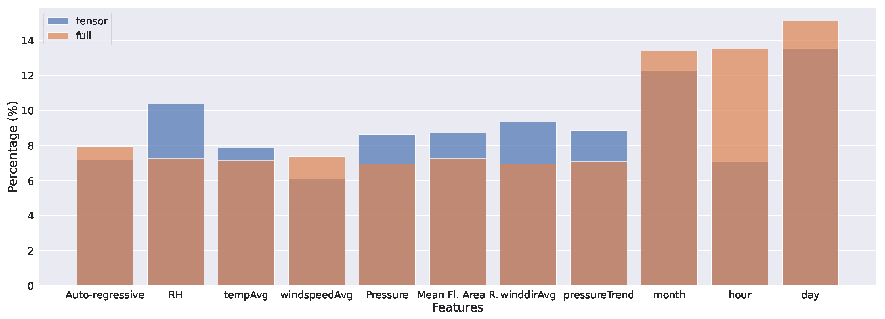
2.2. Feature Selection and Engineering

The spatiotemporal attributes of various PM species, namely, emission rate, concentration distribution and residence time, are influenced by numerous parameters. These influences are shaped by intricate dynamical, thermodynamical and chemical processes. In the literature, one usually utilizes all meteorological features that installed sensors can measure, with temperature, wind velocity and dew point being the most common, among others [30,31,60]. In what follows, we elaborate on the physical reasoning behind the selection of features to be used in our forecasting model, incorporating spatial and temporal features in addition to those of a meteorological nature.

When considering spatial information, commonly used features include coordinates and the distance from a designated point, such as the “city center”, as mentioned in [61]. It is important to note that these features are correlated with the required information but not necessarily causally connected. For instance, the distance from the city center may be correlated with lower population density and, in turn, lower emission rates. However, this consideration can be misleading if there is an industrial facility or if there are extensive agricultural activities in proximity to the sensor, which would contradict the assumption. Moreover, this approach could add challenges in transfer learning approaches from one particular city to another, as the city structure and the local PM emitters’ density could be very different.

A more general approach is to utilize characteristics of the urban structure, namely, the Mean Population Density (MPD) and the Mean Floor Ratio (MFR). The Mean Floor Ratio corresponds to the average ratio of the total built floor area to the area of the specific land under study [62]. It is worth noting that the MFR calculation takes into account the total built floor area, resulting in values larger than 1 for buildings with multiple floors. Urban areas often have higher concentrations of emission sources compared to rural or less densely populated regions. These sources can include vehicular traffic, industrial activities, construction sites, power plants, commercial activities and overall increased energy consumption. As the MFR increases, the density and diversity of emission sources also tend to rise. Consequently, higher PM concentrations can be observed in urban areas due to the greater number and intensity of pollution sources [63]. Moreover, an increased MFR corresponds to increased building capacity, which is closely connected to urban canopy phenomena [64]. In contrast, the MPD represents the average population density within the area where the sensor is located. However, it is important to acknowledge a limitation of the MFR, as it does not account for spaces between buildings, those in particular roads and the percentage of free space between different properties. To address this limitation, additional features, such as road density or the percentage of free space, could be incorporated into the analysis. It should be noted that the MFR corresponds to the legally permitted limits, so it is possible for the actual MFR to be lower (or higher) than the nominal one in certain neighborhoods, considering the specific characteristics of the area. Furthermore, MPD values were estimated using survey data from the Greek Statistical Service. As the survey is performed once per decade, fluctuations are possible. The values of MFR and MPD for the study area were found in [65,66].

Regarding time-related features, their utilization leverages the inherent cyclical and seasonal nature of the phenomenon’s patterns, or the patterns of the features that impact it. Along similar lines to [60], in order to inform the forecasting model about the periodicity of the daily (hours), weekly (days) and seasonal (months) variability of both human-related emissions and also meteorological conditions, we use measurement timestamps; however, we parametrize them differently. In particular, we extract from each timestamp the corresponding hour of the day, $H\in \left\{1,\dots ,24\right\}$, day of the week, $D\in \left\{1,\dots ,7\right\}$, and month of the year, $M\in \left\{1,\dots ,12\right\}$. For each of these, we define two new features:

$$X\_cos=cos\left(\frac{2\pi \times X}{T}\right),X\_sin=sin\left(\frac{2\pi \times X}{T}\right),$$

(1)

where T is equal to 24, 7 or 12 if X corresponds to H, D or M, respectively.

Obviously, meteorological observables also play a crucial role in PM concentration. We begin our discussion with mechanisms that are connected to the dew point which could directly or indirectly affect the PM concentration in the atmosphere [67,68,69]. When an air mass is saturated, water vapor condenses in liquid water droplets, providing a surface for PM to adhere to and thus form larger particles [12]. Furthermore, many particles, including sulfate, nitrate and organic compounds, can undergo gas-to-particle conversion through atmospheric interactions. Consequently, high moisture content in the atmosphere is beneficial for aerosol formation [70]. It should be noted that dew point alone is not an indicator of water vapor content or if the air mass is near saturation. The average dew point is also associated with air mass movements; for instance, changes in dew point can be indicative of the movement and mixing of air masses. When warm, moist air masses encounter cooler air masses or undergo adiabatic cooling due to ascent; the dew point temperature may be reached, leading to the formation of clouds and precipitation. These meteorological conditions can enhance the removal of PM from the atmosphere, effectively reducing its concentration [71]. This effect could result in an overall reduction of the mean PM concentration over the entirety of the studied area. While the dew point provides an absolute measure of the atmospheric moisture content, it does not account for temperature variations that significantly affect the capacity of the air to hold water vapor. For this reason, within our proposed framework, RH is chosen as a feature to capture the relative saturation of the air, which more accurately reflects the moisture dynamics in the varying temperature conditions prevalent in urban microclimates.

Another factor that affects PM concentrations is the air temperature, which modifies the rates of many chemical reactions that lead to the formation of PM [72]. Air temperature also has a significant impact on energy needs within a city. During colder months, increased heating requirements lead to higher energy consumption, often from combustion-based heating systems. Inefficient or poorly maintained systems can contribute to elevated PM emissions [73], while wood combustion also has a significant impact [74]. What is more, during summer, the demand for air conditioning and cooling equipment rises. These systems, relying on electricity often generated from fossil fuels, can indirectly contribute to higher PM emissions [75]. Power generation also plays a crucial role, as extreme temperature events drive increased electricity consumption for heating or cooling. Note that the latter effect is expected to be of diminished importance for the greater Patras area, as the power generation in Greece is centralized and the relative units are located away from the city of Patras. However, in the general case, contributions of local power generation systems could be expected.

Pressure tendency is yet another meteorological observable that can be indirectly correlated to PM concentrations [67,68]. This is because of its connection to synoptic systems. For example, an arriving cyclone (low-pressure system) may induce high wind speeds, cloudy weather and precipitation, resulting in washout and the dispersion of air pollution [76]. In contrast, an inbound anticyclone can result in low wind speeds and atmospheric stability due to the synoptic scale subsidence of air masses. These factors can induce the trapping of air pollution in the lower levels of the atmosphere [77]. Furthermore, atmospheric pressure poses a diurnal fluctuation due to the Earth’s surface heating during daytime and cooling during night-time. On smaller time scales (less than 6 h), pressure may fluctuate due to turbulent flow over complex terrain and big temperature gradients within city landscapes.

It is well established that wind field characteristics, such as wind speed, direction and wind gusts, have a profound impact on the transportation and distribution of air pollution. As a case in point, if the wind blows from an area with significant emissions (for instance industrial zones or agricultural areas) towards a specific location, it can transport and deposit PM, causing an increase in concentration. Conversely, if the wind direction is away from the pollution sources, it can result in lower PM concentrations. Local atmospheric circulation patterns, such as sea breezes, mountain–valley breezes and urban heat island effects, can also impact the dispersion of PM [78]. For example, sea breezes can transport pollutants from coastal areas inland, while mountain–valley breezes can trap pollutants in valleys. Strong wind gusts can lift and suspend PM from the ground or other surfaces, leading to increased concentrations in the air. This effect is especially prominent for fine particles (e.g., ${\mathrm{PM}}_{2.5}$) that have a longer atmospheric residence time. Particles that have settled on roads, construction sites, or other surfaces can be resuspended by gusty winds, contributing to short-term increases in PM concentrations [79]. Similarly, if wind gusts are persistent, they contribute to the dispersion of pre-existing PM concentrations in the atmosphere. The variability of the wind speed can serve as a measure of these phenomena. It is worth noting that an engineered feature of importance for our forecasting model is the so-called variance of the wind speed, which is simply defined as the difference between the maximum and minimum speed measured within a time window.

Finally, in any type of forecasting scenario, employing an auto-regressive approach—that is, using past values of the feature one is aiming to forecast—is vital because it acknowledges the inherent interdependence of data points in the feature’s time-series. Additionally, by considering past values in order to determine future states, the model can learn trends or hyper-local effects that are not directly connected to other features; for instance, an increased restaurant density at the location of a sensor cannot be inferred directly from the MPD or MFR. This approach ultimately allows for more accurate and nuanced forecasts.

Table 1. Grouping of the selected and engineered features into one of four categories.

Spatial	Temporal	Meteorological	Auto-Regressive
MFR, MPD	H_cos, H_sin, D_cos, D_sin, M_cos, M_sin	RH, tempAvg, Pressure/pressureTrend, windGustAvg, windSpeedAvg, windDir_cos, windDir_sin, windSpeedVariance	Auto-regressive

summarizes the used features by their code names, while also grouping them into each of the aforementioned four categories.

2.3. Dataset Development

The target feature corresponds to PM concentration measurements in units of $\mathsf{\mu }$g/m${}^3$, measured by PurpleAir PA-II sensors [49,80] and spanning the time range from 1 December 2018 to 19 June 2022. Historical data are publicly available through the PurpleAir API [81] and were accessed via [82]. The contribution per sensor in the total number of PM concentration measurements is depicted in Figure 1.

PurpleAir PA-II devices are equipped with two PMS5003 laser particle counters, referred to as channels A and B, a BME280 environmental sensor and an ESP8266 micro-controller used for communication. The PMS5003 sensors use a principle of measurement based on the alteration of light intensity as particles traverse the measurement cavity. This phenomenon, termed the nephelometric response, has a direct correlation with the particle concentration, both by mass and number. The algorithm-transforming particle counts in concentration values are proprietary and can therefore be considered to be part of the inherent measurement process. As has been stressed throughout this work so far, the presented framework is sensor-agnostic; nonetheless, and even though PurpleAir provides data for ${\mathrm{PM}}_{1.0}$, ${\mathrm{PM}}_{2.5}$ and ${\mathrm{PM}}_{10}$ concentrations, we opt to work only with ${\mathrm{PM}}_{2.5}$ in what follows because the calibration curves for ${\mathrm{PM}}_{1.0}$ and ${\mathrm{PM}}_{10}$ have not yet been made available [74,83,84]. The code name for the ${\mathrm{PM}}_{2.5}$ data obtained through PurpleAir’s API is pm2.5_cf_1_i, where i corresponds to the channel index and is either A or B, and cf_1 indicates uncorrected values, which are considered to be more robust [74,83].

A pivotal part of our framework is the pre-processing of the data coming from the two sensor channels in order to extract the final concentrations that are used as data points in our study. First, the sensitivity of the sensors is bounded below by applying a consistency condition between the two channels as per the following criterion:

$$\frac{|{\mathrm{PM}}_{A,2.5}-{\mathrm{PM}}_{B,2.5}|}{{\mathrm{PM}}_{A,2.5}+{\mathrm{PM}}_{B,2.5}}\le \alpha \%,$$

(2)

where ${\mathrm{PM}}_{A,2.5}\equiv$ pm2.5_ cf_ 1_A and ${\mathrm{PM}}_{B,2.5}\equiv$ pm2.5_ cf_ 1_B. Following [84], the value $\alpha =30.5$ was selected.

In order to assess the linearity between two channels, we employ Spearman’s and Pearson’s rank-order correlation coefficients, as implemented in the open-source Python library SciPy [85]. Both criteria are non-parametric measures of the monotonicity of the relationship between two variables and $r_k\in [-1,+1]$, where k corresponds to either Pearson or Spearman, with 0 implying no correlation, +1 positive correlation and −1 negative correlation. The difference between the Spearman and Pearson correlation coefficients lies in their underlying assumptions, with the most notable one being normality for the case of Pearson’s coefficient [86]. The corresponding p-value quantifies the probability of the same or more extreme r value to appear due to random fluctuations between uncorrelated datasets. The results can be seen in

Table 2. General properties of our dataset. The id column corresponds to each sensor’s id in the PurpleAir network; N is the total number of data points per sensor; a and b are the coefficients of the linear fit between the channels; and ${\mu }_{\mathrm{scatter}}$, ${\sigma }_{\mathrm{scatter}}$ and $\tilde{\mu }$, ${\sigma }_{\mathrm{median}}$ are mean scatter and median, respectively, with the corresponding standard deviations. Scatter is defined as the orthogonal distance between each $({\mathrm{PM}}_{2.5,channelA},{\mathrm{PM}}_{2.5,channelB})$ value and the fitted line. Moreover, $r_k$ and the corresponding p-values are measures of correlation, with k being either Pearson or Spearmann. Detailed description can be found in the text.

id	N	a	b	${\mathit{r}}_{\mathbf{pears}}$	${\mathit{p}}_{\mathbf{pears}}$	${\mathit{r}}_{\mathbf{spear}}$	${\mathit{p}}_{\mathbf{spear}}$	${\mathit{\mu }}_{\mathbf{scatter}}$	${\mathit{\sigma }}_{\mathbf{scatter}}$	$\tilde{\mathit{\mu }}$	${\mathit{\sigma }}_{\mathbf{median}}$
741	17,467	0.93	−0.77	0.9980	0.0	0.9949	0.0051	2.25	6.19	0.70	0.45
749	25,857	0.94	−0.79	0.9970	0.0	0.9947	0.0053	1.23	3.36	0.59	0.32
1030	5389	0.81	−1.20	0.9752	0.0	0.9714	0.0286	7.71	17.93	3.31	9.75
1566	29,080	0.96	−0.28	0.9970	0.0	0.9970	0.0030	0.69	4.38	0.36	0.12
1672	30,835	1.08	0.06	0.9980	0.0	0.9955	0.0045	1.33	4.25	0.49	0.23
1712	29,580	1.04	0.52	0.9968	0.0	0.9959	0.0041	2.08	11.48	0.65	0.41
5078	26,040	1.00	0.15	0.9984	0.0	0.9965	0.0035	1.45	7.88	0.57	0.31
5092	22,542	0.94	0.37	0.9985	0.0	0.9970	0.0030	2.33	10.03	0.53	0.27
14857	25,990	1.05	−0.61	0.9986	0.0	0.9976	0.0024	1.68	7.57	0.59	0.32
14877	23,250	0.97	−0.42	0.9991	0.0	0.9979	0.0021	1.12	2.84	0.43	0.18
23759	22,756	1.03	0.21	0.9975	0.0	0.9943	0.0057	2.00	9.38	0.49	0.23
30765	18,232	0.99	−0.44	0.9971	0.0	0.9970	0.0030	0.89	8.33	0.33	0.10
56113	10,647	0.98	0.69	0.9958	0.0	0.9942	0.0058	1.66	4.91	0.56	0.29
56229	8001	1.05	0.45	0.9982	0.0	0.9945	0.0055	1.87	13.43	0.72	0.49
56453	10,632	0.86	−0.54	0.9992	0.0	0.9951	0.0049	2.18	11.71	0.44	0.19
57523	5367	0.99	−0.49	0.9997	0.0	0.9991	0.0009	0.82	4.84	0.35	0.12
101589	5248	1.01	−1.02	0.9997	0.0	0.9988	0.0012	1.25	3.05	0.58	0.31
101597	5791	1.11	0.02	0.9980	0.0	0.9980	0.0020	1.32	7.72	0.48	0.22
101609	4927	1.08	0.11	0.9994	0.0	0.9989	0.0011	1.62	6.11	0.48	0.22
101611	7516	0.91	0.74	0.9956	0.0	0.9978	0.0022	2.98	37.17	0.56	0.29
146920	1154	0.91	−0.33	0.9956	0.0	0.9957	0.0043	0.60	0.93	0.29	0.08

. We deduce that both criteria (Pearson and Spearman) strongly support linearity between the two channels, at least on the region where the vast majority of the measurements lie.

As a further step, we perform a linear fit between the two channels and calculate the orthogonal distances between each $({\mathrm{PM}}_{2.5,channelA},{\mathrm{PM}}_{2.5,channelB})$ point and the fitted line:

$${\mathrm{PM}}_{B,2.5}=a\times {\mathrm{PM}}_{A,2.5}+b.$$

(3)

The parameters of the fit are also given in Table 2 for all sensors. In the same table, we also present some statistical measures, namely, the mean value per sensor, the corresponding standard deviation and the median with its dispersion measure. From the difference between mean and median values in Table 2, we deduce the existence of outliers, in agreement with [74]. In order to construct the final ${\mathrm{PM}}_{2.5}$ measurements to be used by our model, we take the weighted average within 1 h, where for weights we use the reverse of the orthogonal distance mentioned before. In this way, we address the fact that the normality of the PM measurements within the 1 h interval cannot be safely assumed in general [87], while we also reduce the impact of outliers. Moreover, we apply a quality cut-off; that is, we exclude measurements where the scatter is more than 1 $\mathsf{\mu }$g/m${}^3$. After this step, we construct the ${\mathrm{PM}}_{2.5,chan.avg}$ measurements as the mean value between the two channels:

$${\mathrm{PM}}_{2.5,chan.avg}=({\mathrm{PM}}_{B,2.5}+{\mathrm{PM}}_{A,2.5})/2.$$

(4)

Finally, as a standard practice for employing data from low-cost sensor networks [74,84,88,89], we apply a calibration procedure. Note that, in general, our pipeline does not depend on the calibration curve used, as it can be applied on the predictions of our model. However, in this case, a sub-part of the trained model will yield results about the physics of the sensor. For example, it has been observed that RH could impact PM measurements in the case of PA-II sensors, e.g., [84]. If the model is trained using uncalibrated data, the latter effect will be captured by it; however, discrimination between PM physics and measurement effects could not be possible.

Among the various linear and non-linear calibration curves employed in the literature (see, e.g., [84]), we choose to use the calibration curve proposed by [84], which reads as

$${\mathrm{PM}}_{2.5,final}=0.524·{\mathrm{PM}}_{2.5,chan.avg}-0.0862·\mathrm{RH}+5.75,$$

(5)

where RH is the relative humidity in %, calculated using the following expression [90]:

$$\mathrm{RH}=exp\left\{\frac{ab\left(T_{DP,avg}-T_{avg}\right)}{\left(T_{avg}+b\right)\left(T_{DP,avg}+b\right)}\right\}\times 100,$$

(6)

where $a=17.368$; b = 238.88 ${}^{\circ }$C; and $T_{avg}$ and $T_{DP,avg}$ are temperature and dew point temperature averages within 1 h.

It is important to note at this point that meteorological variables, specifically pressure, temperature and relative humidity, are measured via the BME280 sensor. Notably, the placement of this sensor directly above the PMS5003 sensors introduces an inherent bias, as heat dissipation from the sensors elevates the temperature readings (from 2.7 ${}^{\circ }$C up to 5.3 ${}^{\circ }$C) and indicates drier RH values (ranging from +9.7% to +24.3%) [89]. This influence is not a static shift but rather a dynamic fluctuation, potentially augmenting or attenuating the physical effects on the data. Moreover, as reported by [84], the dataset exhibits non-physical extrema in temperature and relative humidity, occurring in roughly 1 out of every ${10}^7$ measurements. These are ascribed to electronic noise or communication mishaps between the BME280 sensor and the micro-controller. Anomalously negative temperatures, i.e., around −230 ${}^{\circ }$C, were observed for some of the older sensors used in this study, such as the sensor with id 741.

For the reasons outlined above, and in alignment with other works in the literature [88], the BME280 sensor’s meteorological measurements are excluded from our study. Instead, we utilize open-source data from WeatherUnderground meteorological stations [91], accessed via [92]. The spatial relationship between PM and meteorological sensors is illustrated in Figure 2, while, for completeness, all the labels and descriptions for the available data from the WeatherUnderground sensors can be found in

Table A1. The available observables from the WeatherUnderground sensors network [91].

Label	Unit	Description
Solar Radiation High	W/m${}^2$	High intensity of solar radiation.
uv-High	-	High level of ultraviolet (UV) radiation.
Humidity Low	-	Low humidity level.
Humidity High	-	High humidity level.
Humidity Average	-	Average humidity level.
Temperature High	${}^{\circ }$C	High temperature.
Temperature Low	${}^{\circ }$C	Low temperature.
Temperature Average	${}^{\circ }$C	Average temperature.
Wind Speed High	m/s	High wind speed.
Wind Speed Low	m/s	Low wind speed.
Wind Speed Average	m/s	Average wind speed.
Wind Gust High	m/s	High gusts of wind.
Wind Gust Low	m/s	Low gusts of wind.
Wind Gust Average	m/s	Average gusts of wind.
Wind Direction	deg	Wind Direction.
Dew Point High	${}^{\circ }$C	High dew point temperature.
Dew Point Low	${}^{\circ }$C	Low dew point temperature.
Dew Point Average	${}^{\circ }$C	Average dew point temperature.
Wind Chill High	${}^{\circ }$C	High wind chill temperature.
Wind Chill Low	${}^{\circ }$C	Low wind chill temperature.
Wind Chill Average	${}^{\circ }$C	Average wind chill temperature.
Heat Index High	${}^{\circ }$C	High heat index temperature.
Heat Index Low	${}^{\circ }$C	Low heat index temperature.
Heat Index Average	${}^{\circ }$C	Average heat index temperature.
Pressure Maximum	hPa	Maximum atmospheric pressure.
Pressure Minimum	hPa	Minimum atmospheric pressure.
Pressure Trend	hPa	Difference of atmospheric pressure between subsequent measurements.
Precipitation Rate	mm/h	Rate of precipitation.
Precipitation Total	mm	Total amount of precipitation.

of Appendix A. Regarding the co-location of meteorological stations and PM sensors, we employ an aggregation method along similar lines to [93,94]. Specifically, a scalar meteorological observable Z at the location of PM sensor j is estimated as

$$Z_j=\sum _{i=1}^k{w}_{ij}{Z}_i,$$

(7)

where the weights $w_{ij}=C/l_{ij}$ modulate the influence of each meteorological station. In this expression, $l_{ij}$ is the distance between meteorological station i and PM sensor j; $C={\sum }_{i=1}^{k}1/l_{ij}$ is a normalization constant; and k is the total number of meteorological stations. Specifically for the wind speed and wind direction features, we transformed them into scalar values and applied the transformation of Equation (7) as implemented in the MetPy Python library [95,96].

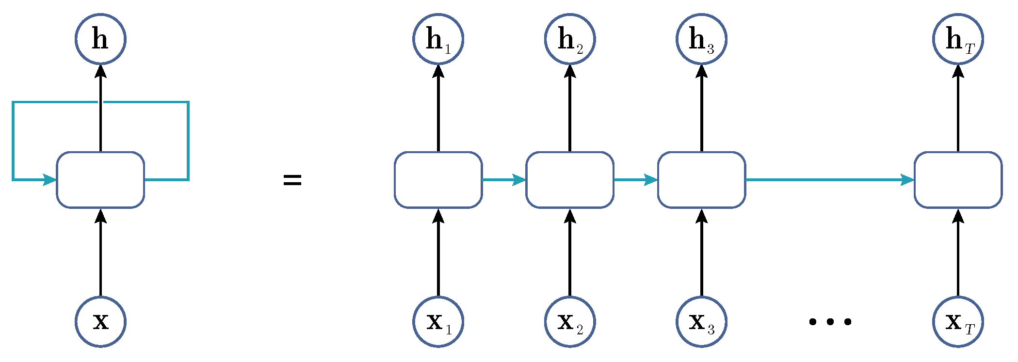
2.4. Forecasting Model Details

In our work, the spatiotemporal variability of PM concentration is modeled via LSTMs. Notably, we use a LSTM instance for the whole city, rather than one instance per sensor, for example, as conducted in [25,97]. In the literature, the spatial variability of the PM concentration has been encapsulated via a variety of approaches [25,26,35,41,42,98]. For instance, the authors in [25] used a Multi-Layer Perceptron (MLP) to combine the results of particular LSTM instances that were used per sensor, while [98] utilized LSTMs for the understanding of the local air pollution dynamics in their area of study. Along similar lines, the authors in [26,35] employed a Convolutional Recurrent Neural Network (CRNN), where geospatial features such as longitude, latitude and distance from city center were fed to CNN layers, and their output was fed to LSTM layers that produced the final prediction. In general, several works in the field utilize combinations of CNN with LSTM networks, such as the approach presented in [35]. Recently, a number of works that employ Gated Recurent Units (GRU), along with CNN [42] or in a encoder–decoder context, have appeared [41].

Finally, there are a few works in the field that employ some sort of “interpretable AI” approach for PM pollution modeling. In particular, at [42], cyclical feature removal was performed and the model’s accuracy was discussed in correlation with the removed feature. A drawback of this approach is that it overlooks the inherent non-linearity of the phenomenon and the persistent interrelationships among features, with the more striking example being those among thermodynamic variables. A more prominent approach on the matter employs Layer-wise Relevance Propagation [41], resulting in so-called importance heat-maps. However, in the latter work, they only considered the prediction range up to 48 h ahead and data from one sensor only, so they do not need to address spatial dependency in their particular context.

While most of these approaches are very suitable for the task at hand, it is important to note that they introduce increased complexity, especially when addressing spatial dependence. This latter fact could seriously affect their generalization ability as the prediction timescale increase [35]. In contrast, our approach addresses spatial dependence through the features discussed in Section 2.2 in order to directly capture the underlying physics of the pollution production and dispersion.

LSTMs [99] fall under the category of Recurrent Neural Networks (RNNs) [100,101] and, as such, they demonstrate exceptional performance in tasks that require the processing of sequential data, including language translation, speech recognition and time-series forecasting [102]. In complete analogy with vanilla RNNs, the recurrent structure of LSTMs can be visualized as a single cell unrolled through time, with each element of the input sequence processed consecutively. In the context of time-series inputs, given a sequence of T time steps $\mathbf{x}=\left\{{\mathbf{x}}_1,\dots ,{\mathbf{x}}_T\right\}$, where ${\mathbf{x}}_t\in {\mathbb{R}}^d$ is the d-dimensional feature vector at time step t, this indicates that the time-series is processed in ascending time step order, as demonstrated in Figure 3.

The output of an LSTM at each time step, t, is a vector known as its hidden state, ${\mathbf{h}}_t$. The key difference between vanilla RNNs and LSTMs is that the information that is passed from time step $t-1$ to time step t is not limited to the hidden state vector ${\mathbf{h}}_{t-1}$; it also includes an additional vector known as the cell state, ${\mathbf{c}}_{t-1}$. The cell state essentially retains and stores important information from past inputs across time steps, allowing the network to “remember” and utilize relevant long-term dependencies (hence the name LSTM).

To compute the hidden and cell state vectors at time step t, the corresponding hidden state vector at time step $t-1$ and the input feature vector ${\mathbf{x}}_t$ undergo independent filtering through three gates, namely, the forget gate, the input gate and the output gate, each of which applies a non-linearity as their activation function. The forget gate determines which information from ${\mathbf{c}}_{t-1}$ should be discarded, while the input gate determines the new information from the input feature vector ${\mathbf{x}}_t$ that should be incorporated into the new cell state, ${\mathbf{c}}_t$. As far as the output gate is concerned, it regulates the information encoded in ${\mathbf{c}}_t$, which propagates into the next time-step’s cell as the hidden state vector, ${\mathbf{h}}_t$.

In their recent study, [44] introduced a novel LSTM variant called Interpretable Multi-Variable LSTM (IMV-LSTM), with the aim of achieving a balance between high forecasting accuracy and offering interpretability for the model’s outputs. In conventional LSTM networks, the hidden state vector captures information from all input features at each time step, which poses challenges in explicitly capturing the unique dynamics of individual features and their interactions. The IMV-LSTM addresses this by extending the concept of the hidden state, generating a hidden state vector for each input feature and employing a novel mixture attention mechanism. Specifically, this mechanism involves applying temporal attention to the sequence of hidden state vectors $\left\{{\mathbf{h}}_1^f,\dots ,{\mathbf{h}}_T^f\right\}$ corresponding to feature f to obtain a summarized history for this feature. Subsequently, using the summarized histories for all features, an additional attention mechanism extracts feature-wise attention scores, which, in turnm can provide insights into each feature’s contribution to the model’s predictions, as well as inter-feature correlations.

As far as the IMV-LSTM model’s implementation is concerned, two alternatives are presented by [44] and both are followed in our work for completeness. The IMV-Full approach essentially corresponds to extending the vectors involved in the traditional LSTM equations into matrices, where each row corresponds to a single feature. The IMV-Tensor approach is equivalent to a set of LSTM networks running in parallel, with each network processing only one input feature’s sequence and then merging all results through the mixture attention mechanism. The code written for the implementation of the models in Python utilizes the PyTorch [103] framework and is heavily influenced by [104].

We construct two feature sets for the case of hourly prediction, namely, “Basic” and “General”. The General feature set contains all the features shown in Table 1, while Basic contains the Pressure feature instead of pressureTrend and does not contain windGustAvg and windSpeedVariance. Moreover, Basic contains only the MFR feature instead of both MFR and MPD. The latter features are corelated to some degree; therefore, using one of them instead of both allows for reducing the total number of features. We point out that the General feature set takes into account the involved physics better than the Basic; however, the reduced feature number allows for faster training. Thus, we use the Basic feature set in order to assess differences between the two IMV-LSTM algorithms in terms of feature importance, while we use the General one in order to achieve the smallest possible RMSE error. We also construct an additional feature set, corresponding to daily predictions, which contains the same features as the General, hourly one, with the obvious exception of H_cos and H_sin.

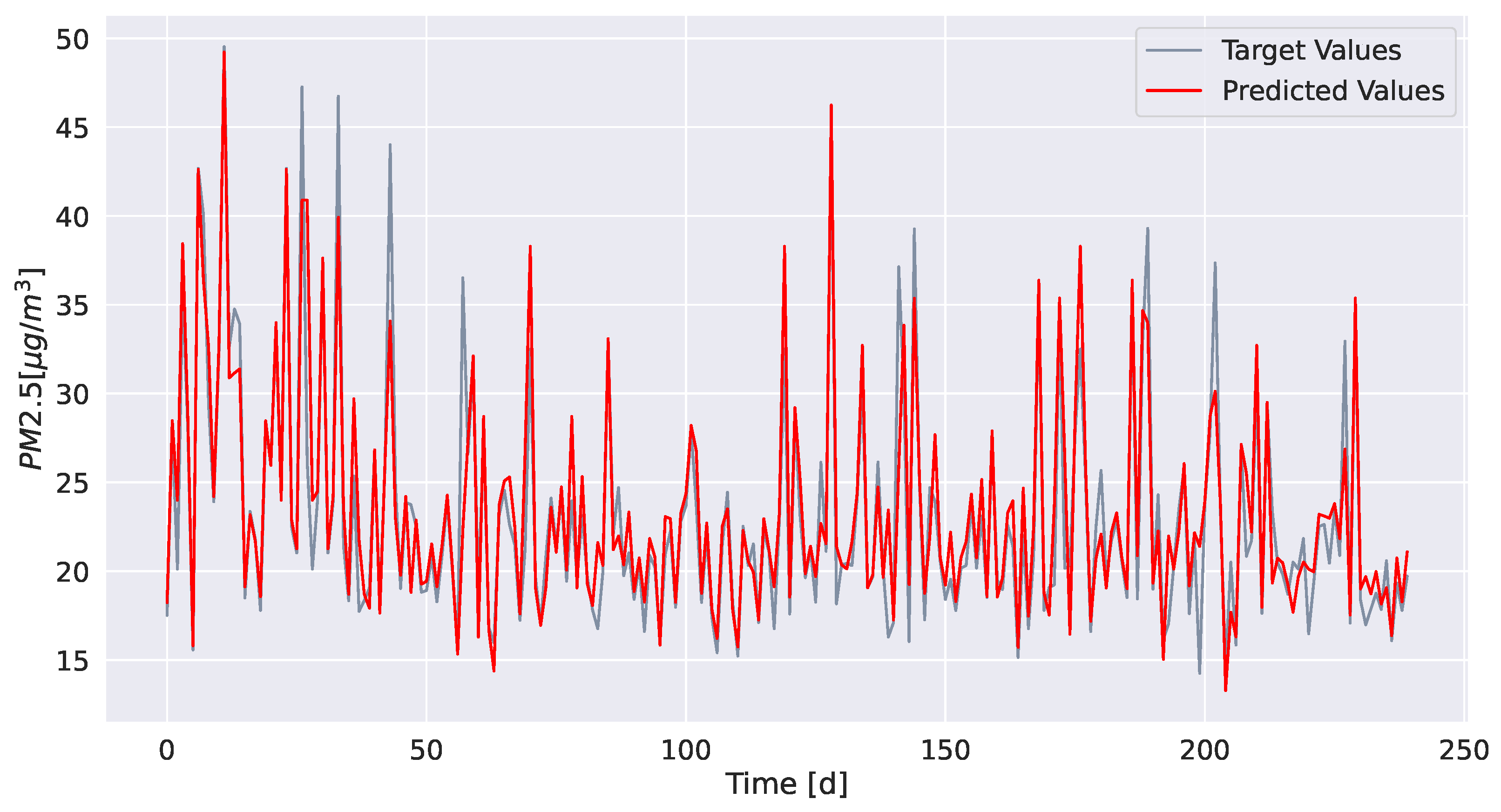
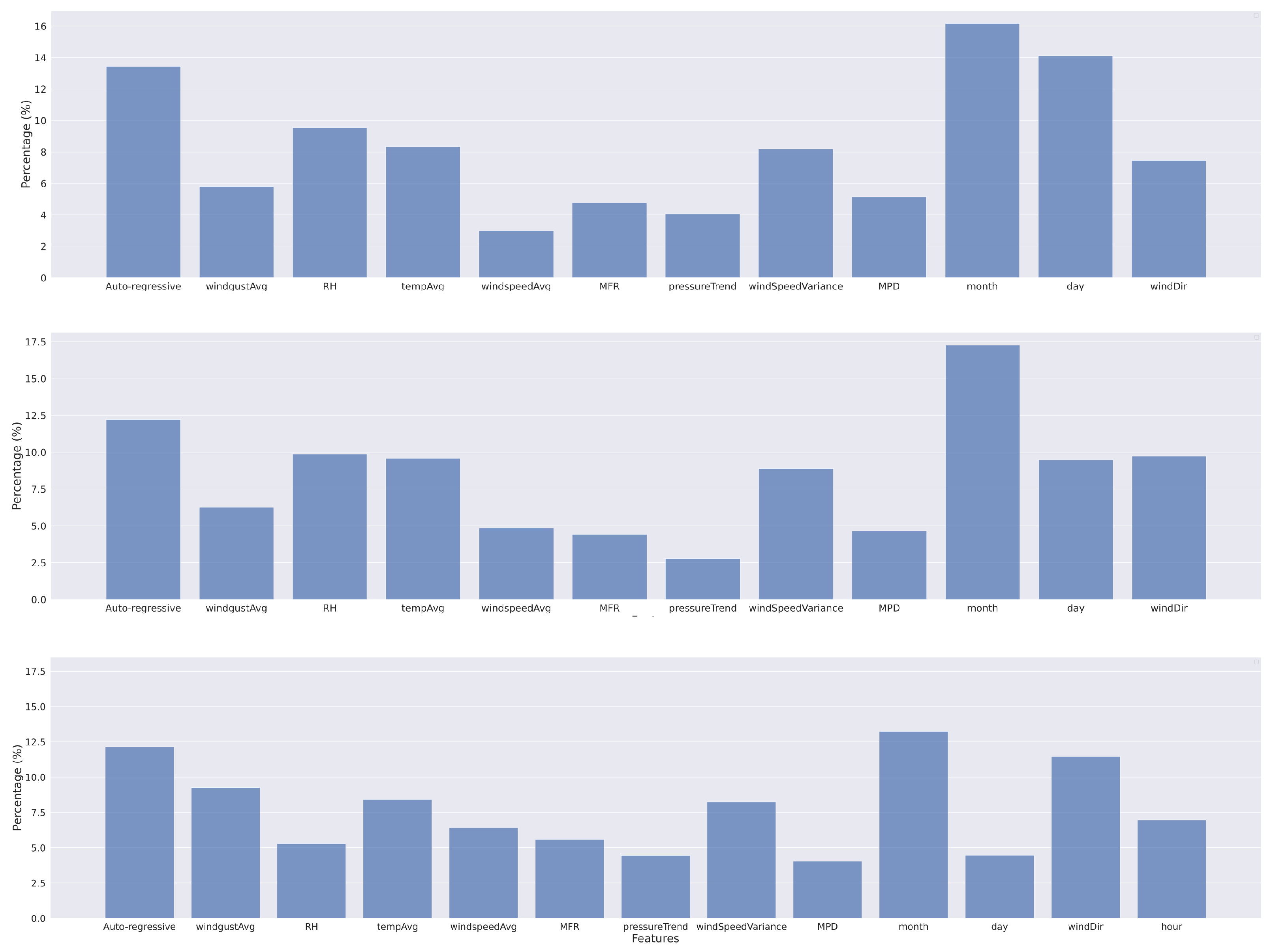
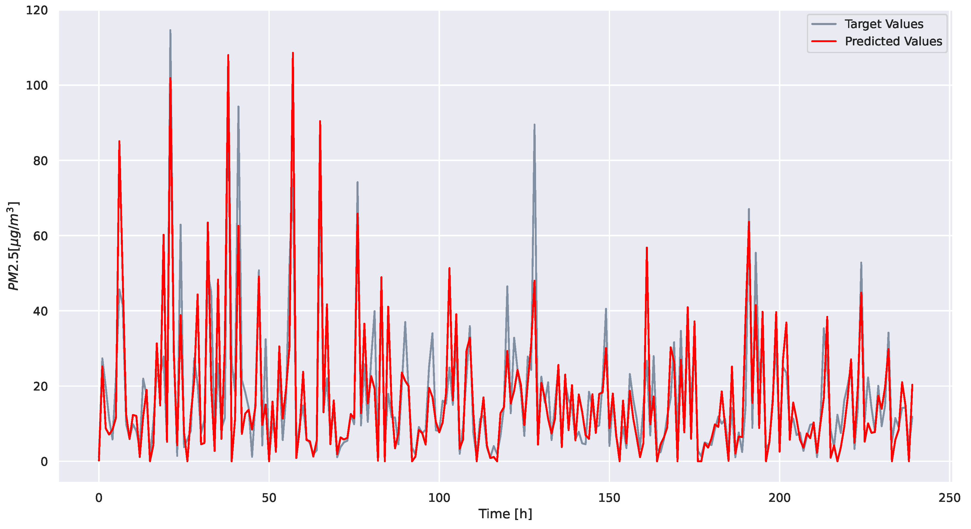
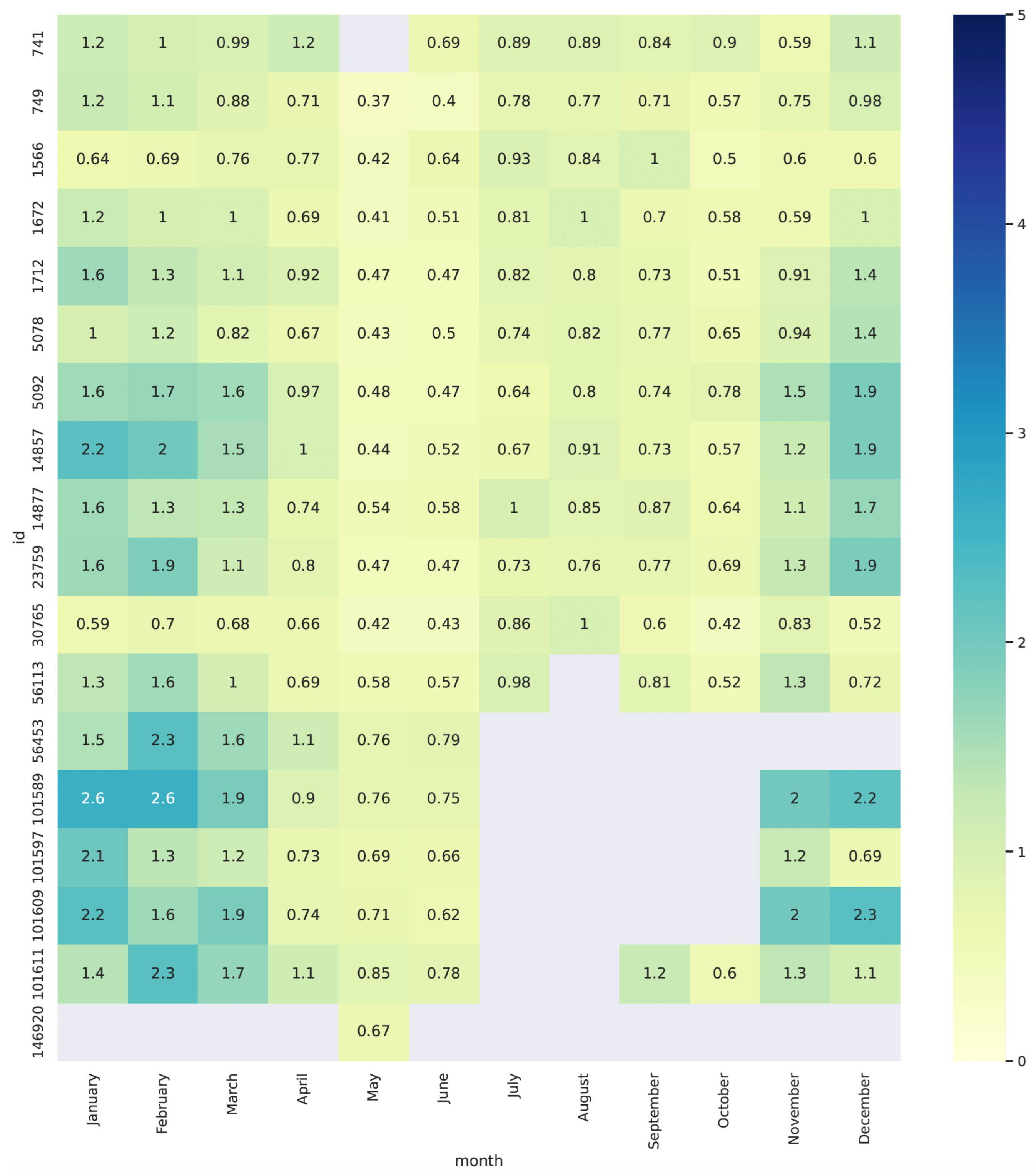
3. Results and Discussion

We use the dataset described at Section 2.3 and, according to standard practice (e.g., [35]), we scale it via standard minmax scaling on $[-1,1]$ space, with the exception of time stamps and wind direction. The latter are transformed via sine/cosine in order to maintain time differences and angular distances between directions, respectively. As standard practice, we split the dataset to three parts, i.e., “train”, “validation” and “test” data, with proportions 50%, 30% and 20%, respectively. We ensure that there is a proportional representation for each sensor and for each timestamp (with emphasis on monthly scale) in the training/test/validation datasets. We set “batch size” to 128 and used 128 LSTM cells. We employed a stopping condition, which it is governed via the “patience” parameter. The latter corresponds to the epochs of training allowed after an increment on the validation error. Along standard lines, we employ Root Mean Square Error (RMSE) as loss function. We use the Adam optimizer, as implemented on the PyTorch package. The relevant parameter values and results are depicted in

Table 3. Results after training for different model and training parameters. Each row refers to a particular model and training setup that has been used for 25 training runs. We have used 600 training epochs, and the “patience” parameter of the early stopping mechanism has been set to 30. The feature sets are defined in the previous section. We present the mean values and standard deviations (std) for Root Mean Squared Error (RMSE) and Mean Absolute Error (MAE).

N/A	Features	Look-Back Time Window	Predict Window	Learning Rate (${10}^{-3}$)	$\mathit{\gamma }$	Steps	RMSE	MAE
1	General—hourly	24 h	24 h	7	0.5	45	$28.0\pm 3.0$	$3.1\pm 0.4$
2	General—hourly	24 h	24 h	5	0.5	45	$23.0\pm 3.5$	$2.8\pm 0.6$
3	General—hourly	24 h	24 h	4.5	0.5	65	$\mathbf{20}.\mathbf{2}\pm \mathbf{1}.\mathbf{3}$	$\mathbf{2}.\mathbf{6}\pm \mathbf{0}.\mathbf{8}$
4	Basic—hourly	48 h	24 h	20	0.5	35	$24.5\pm 2.3$	$2.4\pm 0.6$
5	Standard—daily	7 d	7 d	5	0.5	55	$17.8\pm 1.3$	$3.0\pm 0.4$
6	Standard—daily	24 d	10 d	5	0.5	55	$12.1\pm 1.7$	$2.4\pm 0.8$

. For the case of daily predictions, we resampled our dataset over 24 h and used the median value.

As a first step, we compared the two implementations of IMV-LSTMs from [44] for 25 training runs in terms of their predictive power and the corresponding feature importance. The results on the feature importance are presented in Figure 4. In order to construct the “mean” value on the feature importance, we minimized the following expression:

$$\mathcal{L}\left(f_{mean}\right)={\left(\sum _{j=1}^N\frac{1}{RMS{E}_j}\right)}^{-1}\sum _{j=1}^N\frac{1}{RMS{E}_j}\sqrt{\sum _{i=1}^k{\left(f_{ij}-f_{i,mean}\right)}^2}+\left(\sum _{i=1}^k{f}_{i,mean}-1\right)\times {10}^{\lambda },$$

(8)

where k is the length of the feature importance vector and $RMS{E}_j$ is the RMSE corresponding to this particular run. The first term is the weighted average of the Euclidian distances on the feature space between feature importance vector j and the “mean’’, and as weights, we use the inverse RMSE values. The second term corresponds to the condition that all percentages add to 1. The $\lambda$ parameter is an arbitrary integer, and we set $\lambda =5$ for this set of experiments. We used the feature set and parameters in line 3 of Table 3, and the forecast window has been set to 48 h. The equivalence of feature importance between the two implementations becomes apparent through the mean value estimation of an ensemble of training runs (Figure 4) where the two implementations yield similar importance assessments for each feature. However, this equivalence is statistical in nature due to strong correlations between the features and also the random initialization of LSTMs weights. The latter leads to different convergence rate per feature. As the RMSE error for “tensor” implementation is slightly better than the corresponding one for “full” implementation most of the time, we choose to use the former as the main prediction model. However, we note that the two implementations were found to be almost indiscriminate regarding RMSE loss; moreover, their feature importance assessments are statistically equivalent.

For the case of daily predictions, we trained and validated two models. In particular, a model with prediction window of 7 days and another one with a prediction window of 10 days. The validation results for daily predictions are depicted in Figure 5. In the upper panel of Figure 6, the feature importance for the model trained for daily predictions, averaged over 25 runs is presented. All sin/cos parametrized features (time and wind direction features) has been summed, resulting in “month”, “day” and “windDir”, respectively. We observe that the features that contribute most to the prediction, in order of decreasing importance, are “month”, “day”, “Auto-regressive”, “RH”, “tempAvg”, “windSpeedVariance”, “winddirAvg”, “windgustAvg”, “MPD”, “MFR”, “pressureTrend” and “windSpeedAvg”. The major contribution of the “month” feature can be related to the summer/winter difference on local emissions due to residential heating. The importance of the “day” feature for the prediction points out to the significant variability of the emissions within the week, which underlines the relative importance of local sources variability, such as vehicle traffic and restaurants. Of course, the latter areas could be otherwise indistinguishable with regard to “MPD” and “MFD” features. This could also explain the relatively small importance of “MPD” and “MFD” features in comparison with “Auto-regression”. The “RH” and “tempAvg” features are generally related with the stability of ABL; however, there are some differences. In particular, the “tempAvg” is correlated with summer/winter variability, while the “RH” is also related with the physics of the sensors, as their sensitivity is closely connected with the humidity, e.g., [84]. Furthermore, the perception of coldness in humans is influenced by a combination of factors, including humidity, wind speed, and, of course, temperature. This sensation of coldness potentially affects the decision to activate heating systems during the colder months of the year. The greater significance of “windSpeedVariance” and “windDir” compared to just “windSpeedAverage” suggests the influence of the urban structure. The former two features are associated with the formation and lifetime of coherent turbulent structures within the intricate urban layout. Moreover, as there exist important intra-city variability of the emissions (e.g., [105]), pollution transport from higher polluted areas towards areas with lower density could result increased importance of the wind direction. This interpretation is in alignment with the results of [39]. Another possibility for the contribution of wind direction is through dust transport events [57], as the latter are frequently occuring from south to southwest. A difference between the aforementioned mechanisms pertains to the relevant timescale, as the former mechanism operates on shorter timescales, while the latter on larger ones.

Apart from daily means, in order to be able to provide meaningful information to the general public, i.e., to allow for optimal scheduling the daily chores, a hourly prediction model is imperative. The validation plot (Figure 7) shows very good agreement between the predicted and the actual values. A rather interesting observation is with regard to the peak height. Specifically, while the trained model correctly captures the position of each peak (or low point) almost every time, there are cases where the height (depth) of the peak (low point) are not captured. This could be attributed to the extreme time-variable contribution of traffic emissions. The increment of the “pressureTrend” feature’s importance for the hourly predictions model compared to daily prediction models (e.g., compare the upper panel of Figure 6 with the lower panel of the same Figure) points to the increased impact of atmospheric mixing on the phenomenon. Regarding feature importance, we observe in lower panel of Figure 6 that the features that contribute most to the prediction, in order of decreasing importance, are “month”, “Auto-regressive”, “windDir”, “windgustAvg”, “tempAvg”, “windSpeedVariance”, “hour”, “windSpeedAvg”, “MFR”, “RH”, “pressureTrend”, “day” and “MPD”. The increased importance of “windDir”, “windgustAvg” and “windSpeedVariance” features with regard to the daily prediction models discussed previously could be interpreted as caused by the increased importance of turbulent coherent structures on hourly (and lower) timescales for PM dispersion. Note also the increment of the “MFR” feature’s importance in comparison with the corresponding value from the daily prediction model. The latter, although small (∼2%), is another indicator of the above mechanism. A rather interesting observation pertains to the reduction of the “day” feature’s importance, where there is a ∼5% reduction. The latter could be caused by the large difference between the variance of PM concentration with respect to the hourly and daily scales. The latter variability in the concentration far exceeds the magnitude of the weekly variability in light of the RMSE; therefore, the impact of the “day” feature on the predictive ability of the hourly model is reduced.

The MAE error distribution of the model per month and and per sensor is presented in Figure 8. First of all, we note that the mean error per sensor per month is less that $3\sigma$, i.e., ∼8 $\mathsf{\mu }$g/m${}^3$. Moreover, we observe higher errors (more blue hues) regarding winter months, in comparison to the summer months (more yellow hues). The latter is fully compatible with a similar result reported in [35], regarding Beijing, China. In addition, Ref. [105] reported higher variability on the winter months for the city of Patras and other Greek cities. However there are two sensors, i.e., 1566 and 30765, that deviate from this trend. Both of them are situated in the University of Patras area, which is located on the outskirts of Patras city. It is reasonable to assume that the impact of residential heating in this area is minimal, resulting in no significant increase in prediction errors during winter months. Moreover, the highest error corresponds to sensor 101589, which is located in Lefka, a relatively sparsely populated area engaged in agricultural activities, notably olive/citrus groves and cattle farms. Thus, the peak error in the months of January and February could be attributed to the combined effects of burning agricultural waste and residential heating.

Let us now discuss a rather interesting, overarching insight from our study. By comparing the feature importance assessment between daily and hourly predictions (i.e., the upper and lower panels of Figure 6) we observe that the summer/winter qualitative change on the pollution production and dispersion is described better with the “month” feature than with “tempAvg”. In fact the importance of “month’ is almost two times larger than the importance of “tempAvg” for the daily prediction model, while for hourly prediction model is about 4% larger. Considering the fact that the “tempAvg” corresponds to a fundamental quality regarding residential heating, which constitutes a major pollution source, the opposite was expected. This could be explained by the operation of central heating systems in apartment blocks in Patras city that are set to work for fixed hours per week within the winter, beginning from a starting date [106]. Thus, the aforementioned mode of residential heating does not become “informed” of daily and weekly temperature variations. Unfortunately, the exact percentage of buildings that use central heating systems in Patras is not known. However, we can estimate their number to be around 50% based on a relevant work for the city of Thessaloniki [107] and the fact that Greek cities, in general, followed similar evolutionary path (i.e., excessive growth over similar periods) [108]. Of course, in detail modeling of residential heating is out of the scope of this work. Another point has to do with the emergence of socioeconomic reasons that could cause the periodic non-availability of residential heating (e.g., an increment of the percentage of the salary that is used to cover heating needs) and/or non-optimal working conditions for the boiler (e.g., bad maintenance), which are independent of the temperature.

Concluding this discourse, it becomes imperative to compare our proposed framework with analogous studies within the literature, with emphasis placed on the prediction accuracy. It is noteworthy that direct comparisons in terms of accuracy are inherently intricate due to several factors. These factors encompass data availability regarding the new features we introduce (e.g., MFR, MPD), the utilization of diverse prediction windows, and variations in the geographical settings, which are subject to distinct meteorological dynamics. Regarding prediction accuracy, a study by [97], investigating the same geographic region (though utilizing distinct LSTM instances for each sensor and 6-h averages), delineated a standard deviation (MAE) ranging from approximately ∼2 $\mathsf{\mu }$g/m${}^3$ (during summer) to about ∼6 $\mathsf{\mu }$g/m${}^3$ (during winter) for their projections. When compared with our computed mean absolute errors for both hourly (approximately 3 $\mathsf{\mu }$g/m${}^3$) and daily forecasts (about 2 $\mathsf{\mu }$g/m${}^3$), it is deducible that our framework manifests a marginal improvement in predictive precision for protracted forecasting spans and finer temporal resolutions. Intriguingly, the corresponding mean RMSE error for all LSTM instances cited by [97], namely, ∼5 $\mathsf{\mu }$g/m${}^3$, is two to four times lower than our analogous values (∼12 $\mathsf{\mu }$g/m${}^3$ for daily and ∼20 $\mathsf{\mu }$g/m${}^3$ for hourly models). This observed trend could potentially be attributed to the increased presence of local extreme events within our validation dataset. Notably, the dataset employed by [97] is substantially smaller compared to ours. Specifically, their dataset comprises around 2 years of hourly measurements from 8 sensors, whereas ours spans 3.5 years and encompasses readings from 18 sensors. This dissimilarity in dataset dimensions suggests a relatively diminished occurrence of outliers within their validation data, conceivably leading to a reduced RMSE in their prognostications. Conversely, the lower MAE in our forecasts signifies a slightly superior ability to predict events within the data distribution. Considering the findings of [60], wherein LSTM models for temporal aspects and multi-layer perceptrons for spatial variability were employed, it is evident that our corresponding model exhibits MAE values approximately five times lower than those reported by [60]. Another category of models involves diverse amalgamations of LSTM and CNN cells, as exemplified by studies such as [35,38]. In the latter investigation, RMSE values span approximately ∼20 $\mathsf{\mu }$g/m${}^3$ (for a 1-h prediction window) to surpassing ∼50 $\mathsf{\mu }$g/m${}^3$ (for a 6-h prediction window). In the former, the MAE for PM_2.5 predictions attains approximately ∼11 $\mathsf{\mu }$g/m${}^3$. Both of these figures exceed our achieved results of approximately ∼3 $\mathsf{\mu }$g/m${}^3$. Note that due to the limitations of the above comparison, we can not claim the superiority of our framework over these mentioned models; rather, we contend that our framework necessitates more thorough investigation and broader application across diverse urban contexts, adeptly accommodating the intricacies of varying spatial scales and emission patterns. A recent study by [39] has achieved an impressive prediction accuracy almost ∼1 $\mathsf{\mu }$g/m${}^3$. However, this accomplishment relies heavily upon external datasets, specifically daily satellite data and 3D building models generated from LIDAR observations. It is crucial to emphasize that the global accessibility of these datasets can face limitations due to technical, economic and political factors, which pose a barrier to the widespread applicability of [39]’s approach.

Ultimately, the cost-efficiency of our approach is grounded in the effective utilization of a dataset derived from networks of low-cost sensors, encompassing both PM and meteorological observations, alongside the integration of Free and Open Source (FOSS) tools. Bolstered by the coherent physical interpretation of our model outcomes, we posit that the model aptly captures a substantial portion of the underlying physical mechanisms. Flowing from this insight, we anticipate that, in the context of continuous operation, the requisite retraining frequency could be minimized.

4. Conclusions

PM pollution is associated with increased cardiovascular and respiratory diseases [1]. Climate change is also expected to increase PM concentrations in the near future [109]. It now becomes more critical than ever before to the reduce climate and air quality effects on human health. The proposed prediction model can be considered as an important factor (alongside others) in environmental policy-making. We utilized a novel Long Short-Term Memory Neural Network for predicting PM (particulate matter) concentration in urban environments. Our approach involved using a network of low-cost sensors, which we calibrated using classical methods. We also introduced novel features, namely, the Mean Floor Ratio and population density, along with Wind Speed Variance. We demonstrate the effectiveness of our model through a case study in a Greek port city, where the dense urban environment is combined with a diverse variety of pollution sources. Our approach offers increased flexibility with regard to the literature, i.e., allowing for portable sensors and also for the replacement and/or removal of existing sensors. Note also that our model is completely general as it allows for the integration of different sensor types.

It is important to acknowledge a limitation of the MFR used in the proposed approach, as it does not account for spaces between buildings. To address this limitation, additional features, such as road density or the percentage of free space, could be incorporated into the analysis. Furthermore, since MPD values were estimated using survey data that is recorded once per decade, fluctuations are possible. Notice also that the proposed model provides point predictions, as past values of the measured pollutants on the required position are needed. Finally, in the current setup, the existence of a sensor network is imperative for both PM and meteorological data. In principle, transfer learning approaches could evade at least part of the aforementioned constraints. All these issues and proposed possible interventions are left for future investigation.

To further enhance the predictive capabilities of our framework, future directions will also include the integration of additional information sources; for example, leveraging data from social networks and daily news to address out-of-distribution events and capture fluctuations in human activity, such as large leisure happenings and/or public demonstrations. Another approach of interest is the combination of our model with a transport model such as CAMx, where the latter is employed to address large-scale phenomena such as dust transport. Along with the flexibility necessary to employ different sensor configurations directly, our model can be used as the core component of a comprehensive prediction framework. Along with its accuracy, it has the potential to contribute to effective decision-making and comprehensive pollution management strategies. Finally, as our approach uses FOSS in its entirety along with Open Data from low-cost sensors, it could be a basis for a cost-efficient and widely applicable solution to the problems of pollution forecasting.

References

1. WHO. WHO Global Air Quality Guidelines: Particulate Matter (PM2.5 and PM10), Ozone, Nitrogen Dioxide, Sulfur Dioxide and Carbon Monoxide; World Health Organization: Geneva, Switzerland, 2021. [Google Scholar]
2. Goldberg, M. A systematic review of the relation between long-term exposure to ambient air pollution and chronic diseases. Rev. Environ. Health 2008, 23, 243–298. [Google Scholar] [CrossRef] [PubMed]
3. Khaniabadi, Y.O.; Goudarzi, G.; Daryanoosh, S.M.; Borgini, A.; Tittarelli, A.; De Marco, A. Exposure to PM10, NO2, and O3 and impacts on human health. Environ. Sci. Pollut. Res. 2017, 24, 2781–2789. [Google Scholar] [CrossRef] [PubMed]
4. Coccia, M. The effects of atmospheric stability with low wind speed and of air pollution on the accelerated transmission dynamics of COVID-19. Int. J. Environ. Stud. 2021, 78, 1–27. [Google Scholar] [CrossRef]
5. Coccia, M. How do low wind speeds and high levels of air pollution support the spread of COVID-19? Atmos. Pollut. Res. 2021, 12, 437–445. [Google Scholar] [CrossRef]
6. Akan, A.P.; Coccia, M. Changes of air pollution between countries because of lockdowns to face COVID-19 pandemic. Appl. Sci. 2022, 12, 12806. [Google Scholar] [CrossRef]
7. Kampa, M.; Castanas, E. Human health effects of air pollution. Environ. Pollut. 2008, 151, 362–367. [Google Scholar] [CrossRef]
8. Brunekreef, B.; Holgate, S.T. Air pollution and health. Lancet 2002, 360, 1233–1242. [Google Scholar] [CrossRef]
9. Seinfeld, H.J.; Pandis, N.S. Atmospheric Chemistry and Physics: From Air Pollution to Climate Change; Wiley: Hoboken, NJ, USA, 2016. [Google Scholar]
10. Kaskaoutis, D.; Grivas, G.; Oikonomou, K.; Tavernaraki, P.; Papoutsidaki, K.; Tsagkaraki, M.; Stavroulas, I.; Zarmpas, P.; Paraskevopoulou, D.; Bougiatioti, A.; et al. Impacts of severe residential wood burning on atmospheric processing, water-soluble organic aerosol and light absorption, in an inland city of Southeastern Europe. Atmos. Environ. 2022, 280, 119139. [Google Scholar] [CrossRef]
11. Papadakis, G.; Megaritis, A.; Pandis, S. Effects of olive tree branches burning emissions on PM2.5 concentrations. Atmos. Environ. 2015, 112, 148–158. [Google Scholar] [CrossRef]
12. Levin, Z.; Cotton, R.W. Atmospheric Chemistry and Physics: From Air Pollution to Climate Change; Springer: Berlin/Heidelberg, Germany, 2009. [Google Scholar]
13. Su, T.; Li, Z.; Li, C.; Li, J.; Han, W.; Shen, C.; Tan, W.; Wei, J.; Guo, J. The significant impact of aerosol vertical structure on lower atmosphere stability and its critical role in aerosol–planetary boundary layer (PBL) interactions. Atmos. Chem. Phys. 2020, 20, 3713–3724. [Google Scholar] [CrossRef]
14. Pearlmutter, D.; Bitan, A.; Berliner, P. Microclimatic analysis of “compact” urban canyons in an arid zone. Atmos. Environ. 1999, 33, 4143–4150. [Google Scholar] [CrossRef]
15. Toscano, D.; Marro, M.; Mele, B.; Murena, F.; Salizzoni, P. Assessment of the impact of gaseous ship emissions in ports using physical and numerical models: The case of Naples. Build. Environ. 2021, 196, 107812. [Google Scholar] [CrossRef]
16. Merico, E.; Dinoi, A.; Contini, D. Development of an integrated modelling-measurement system for near-real-time estimates of harbour activity impact to atmospheric pollution in coastal cities. Transp. Res. Part D Transp. Environ. 2019, 73, 108–119. [Google Scholar] [CrossRef]
17. Progiou, A.; Bakeas, E.; Evangelidou, E.; Kontogiorgi, C.; Lagkadinou, E.; Sebos, I. Air pollutant emissions from Piraeus port: External costs and air quality levels. Transp. Res. Part D Transp. Environ. 2021, 91, 102586. [Google Scholar] [CrossRef]
18. Wang, J.; Xing, J.; Mathur, R.; Pleim, J.E.; Wang, S.; Hogrefe, C.; Gan, C.M.; Wong, D.C.; Hao, J. Historical trends in PM2.5-related premature mortality during 1990–2010 across the northern hemisphere. Environ. Health Perspect. 2017, 125, 400–408. [Google Scholar] [CrossRef] [PubMed]
19. Jeanjean, A.P.; Monks, P.S.; Leigh, R.J. Modelling the effectiveness of urban trees and grass on PM2.5 reduction via dispersion and deposition at a city scale. Atmos. Environ. 2016, 147, 1–10. [Google Scholar] [CrossRef]
20. Lauriks, T.; Longo, R.; Baetens, D.; Derudi, M.; Parente, A.; Bellemans, A.; Van Beeck, J.; Denys, S. Application of improved CFD modeling for prediction and mitigation of traffic-related air pollution hotspots in a realistic urban street. Atmos. Environ. 2021, 246, 118127. [Google Scholar] [CrossRef]
21. Hao, C.; Xie, X.; Huang, Y.; Huang, Z. Study on influence of viaduct and noise barriers on the particulate matter dispersion in street canyons by CFD modeling. Atmos. Pollut. Res. 2019, 10, 1723–1735. [Google Scholar] [CrossRef]
22. Tsiaousidis, D.T.; Liora, N.; Kontos, S.; Poupkou, A.; Akritidis, D.; Melas, D. Evaluation of PM Chemical Composition in Thessaloniki, Greece Based on Air Quality Simulations. Sustainability 2023, 15, 10034. [Google Scholar] [CrossRef]
23. Fameli, K.M.; Assimakopoulos, V.D. The new open Flexible Emission Inventory for Greece and the Greater Athens Area (FEI-GREGAA): Account of pollutant sources and their importance from 2006 to 2012. Atmos. Environ. 2016, 137, 17–37. [Google Scholar] [CrossRef]
24. Pérez, P.; Trier, A.; Reyes, J. Prediction of PM2.5 concentrations several hours in advance using neural networks in Santiago, Chile. Atmos. Environ. 2000, 34, 1189–1196. [Google Scholar] [CrossRef]
25. Zhao, J.; Deng, F.; Cai, Y.; Chen, J. Long short-term memory-Fully connected (LSTM-FC) neural network for PM2.5 concentration prediction. Chemosphere 2019, 220, 486–492. [Google Scholar] [CrossRef] [PubMed]
26. Qin, D.; Yu, J.; Zou, G.; Yong, R.; Zhao, Q.; Zhang, B. A novel combined prediction scheme based on CNN and LSTM for urban PM2.5 concentration. IEEE Access 2019, 7, 20050–20059. [Google Scholar] [CrossRef]
27. Zhou, Y.; Chang, F.J.; Chang, L.C.; Kao, I.F.; Wang, Y.S. Explore a deep learning multi-output neural network for regional multi-step-ahead air quality forecasts. J. Clean. Prod. 2019, 209, 134–145. [Google Scholar] [CrossRef]
28. Wu, X.; Wang, Y.; He, S.; Wu, Z. PM2.5/PM10 ratio prediction based on a long short-term memory neural network in Wuhan, China. Geosci. Model Dev. 2020, 13, 1499–1511. [Google Scholar] [CrossRef]
29. Zhang, B.; Zhang, H.; Zhao, G.; Lian, J. Constructing a PM2.5 concentration prediction model by combining auto-encoder with Bi-LSTM neural networks. Environ. Model. Softw. 2020, 124, 104600. [Google Scholar] [CrossRef]
30. Li, T.; Hua, M.; Wu, X. A hybrid CNN-LSTM model for forecasting particulate matter (PM2.5). IEEE Access 2020, 8, 26933–26940. [Google Scholar] [CrossRef]
31. Pak, U.; Ma, J.; Ryu, U.; Ryom, K.; Juhyok, U.; Pak, K.; Pak, C. Deep learning-based PM2.5 prediction considering the spatiotemporal correlations: A case study of Beijing, China. Sci. Total Environ. 2020, 699, 133561. [Google Scholar] [CrossRef]
32. Qiao, W.; Wang, Y.; Zhang, J.; Tian, W.; Tian, Y.; Yang, Q. An innovative coupled model in view of wavelet transform for predicting short-term PM10 concentration. J. Environ. Manag. 2021, 289, 112438. [Google Scholar] [CrossRef]
33. Zhang, L.; Na, J.; Zhu, J.; Shi, Z.; Zou, C.; Yang, L. Spatiotemporal causal convolutional network for forecasting hourly PM2.5 concentrations in Beijing, China. Comput. Geosci. 2021, 155, 104869. [Google Scholar] [CrossRef]
34. Zhang, B.; Zou, G.; Qin, D.; Lu, Y.; Jin, Y.; Wang, H. A novel Encoder-Decoder model based on read-first LSTM for air pollutant prediction. Sci. Total Environ. 2021, 765, 144507. [Google Scholar] [CrossRef] [PubMed]
35. Yan, R.; Liao, J.; Yang, J.; Sun, W.; Nong, M.; Li, F. Multi-hour and multi-site air quality index forecasting in Beijing using CNN, LSTM, CNN-LSTM, and spatiotemporal clustering. Expert Syst. Appl. 2021, 169, 114513. [Google Scholar] [CrossRef]
36. Mao, W.; Wang, W.; Jiao, L.; Zhao, S.; Liu, A. Modeling air quality prediction using a deep learning approach: Method optimization and evaluation. Sustain. Cities Soc. 2021, 65, 102567. [Google Scholar] [CrossRef]
37. Du, M.; Chen, Y.; Liu, Y.; Yin, H. A Novel Hybrid Method to Predict PM2.5 Concentration Based on the SWT-QPSO-LSTM Hybrid Model. Comput. Intell. Neurosci. 2022, 2022, 7207477. [Google Scholar] [CrossRef] [PubMed]
38. Hu, K.; Guo, X.; Gong, X.; Wang, X.; Liang, J.; Li, D. Air quality prediction using spatio-temporal deep learning. Atmos. Pollut. Res. 2022, 13, 101543. [Google Scholar] [CrossRef]
39. Liang, L.; Daniels, J.; Bailey, C.; Hu, L.; Phillips, R.; South, J. Integrating low-cost sensor monitoring, satellite mapping, and geospatial artificial intelligence for intra-urban air pollution predictions. Environ. Pollut. 2023, 331, 121832. [Google Scholar] [CrossRef]
40. Zhao, L.; Zhang, M.; Cheng, S.; Fang, Y.; Wang, S.; Zhou, C. Investigate the effects of urban land use on PM2.5 concentration: An application of deep learning simulation. Build. Environ. 2023, 242, 110521. [Google Scholar] [CrossRef]
41. Mirzavand Borujeni, S.; Arras, L.; Srinivasan, V.; Samek, W. Explainable sequence-to-sequence GRU neural network for pollution forecasting. Sci. Rep. 2023, 13, 9940. [Google Scholar] [CrossRef]
42. Elbaz, K.; Shaban, W.M.; Zhou, A.; Shen, S.L. Real time image-based air quality forecasts using a 3D-CNN approach with an attention mechanism. Chemosphere 2023, 333, 138867. [Google Scholar] [CrossRef]
43. Castelvecchi, D. Can we open the black box of AI? Nat. News 2016, 538, 20. [Google Scholar] [CrossRef]
44. Guo, T.; Lin, T.; Antulov-Fantulin, N. Exploring interpretable lstm neural networks over multi-variable data. In Proceedings of the International Conference on Machine Learning, PMLR, Long Beach, CA, USA, 9–15 June 2019; pp. 2494–2504. [Google Scholar]
45. Kumar, P.; Morawska, L.; Martani, C.; Biskos, G.; Neophytou, M.; Di Sabatino, S.; Bell, M.; Norford, L.; Britter, R. The rise of low-cost sensing for managing air pollution in cities. Environ. Int. 2015, 75, 199–205. [Google Scholar] [CrossRef] [PubMed]
46. CanAirIO. Available online: https://scistarter.org/canairio (accessed on 1 September 2023).
47. Map—PurpleAir. Available online: https://map.purpleair.com/ (accessed on 1 September 2023).
48. Kosmopoulos, G.; Salamalikis, V.; Wilbert, S.; Zarzalejo, L.F.; Hanrieder, N.; Karatzas, S.; Kazantzidis, A. Investigating the Sensitivity of Low-Cost Sensors in Measuring Particle Number Concentrations across Diverse Atmospheric Conditions in Greece and Spain. Sensors 2023, 23, 6541. [Google Scholar] [CrossRef] [PubMed]
49. Kosmopoulos, G.; Salamalikis, V.; Matrali, A.; Pandis, S.N.; Kazantzidis, A. Insights about the Sources of PM2.5 in an Urban Area from Measurements of a Low-Cost Sensor Network. Atmosphere 2022, 13, 440. [Google Scholar] [CrossRef]
50. Hedworth, H.A.; Sayahi, T.; Kelly, K.E.; Saad, T. The effectiveness of drones in measuring particulate matter. J. Aerosol Sci. 2021, 152, 105702. [Google Scholar] [CrossRef]
51. Kaivonen, S.; Ngai, E.C.H. Real-time air pollution monitoring with sensors on city bus. Digit. Commun. Netw. 2020, 6, 23–30. [Google Scholar] [CrossRef]
52. Global Modeling and Assimilation Office (GMAO). MERRA-2 instU_2d_lfo_Nx: 2d, 2d,diurnal, Instantaneous, Single-Level, Assimilation, Land Surface Forcings V5.12.4; Goddard Earth Sciences Data and Information Services Center (GES DISC): Greenbelt, MD, USA, 2023. [Google Scholar] [CrossRef]
53. Fameli, K.; Kotrikla, A.; Psanis, C.; Biskos, G.; Polydoropoulou, A. Estimation of the emissions by transport in two port cities of the northeastern Mediterranean, Greece. Environ. Pollut. 2020, 257, 113598. [Google Scholar] [CrossRef]
54. Manousakas, M.; Papaefthymiou, H.; Diapouli, E.; Migliori, A.; Karydas, A.; Bogdanovic-Radovic, I.; Eleftheriadis, K. Assessment of PM2.5 sources and their corresponding level of uncertainty in a coastal urban area using EPA PMF 5.0 enhanced diagnostics. Sci. Total Environ. 2017, 574, 155–164. [Google Scholar] [CrossRef]
55. Kostenidou, E.; Florou, K.; Kaltsonoudis, C.; Tsiflikiotou, M.; Vratolis, S.; Eleftheriadis, K.; Pandis, S.N. Sources and chemical characterization of organic aerosol during the summer in the eastern Mediterranean. Atmos. Chem. Phys. 2015, 15, 11355–11371. [Google Scholar] [CrossRef]
56. Manousakas, M.; Diapouli, E.; Papaefthymiou, H.; Kantarelou, V.; Zarkadas, C.; Kalogridis, A.C.; Karydas, A.G.; Eleftheriadis, K. XRF characterization and source apportionment of PM10 samples collected in a coastal city. X-Ray Spectrom. 2018, 47, 190–200. [Google Scholar] [CrossRef]
57. Matthaios, V.N.; Triantafyllou, A.G.; Koutrakis, P. PM10 episodes in Greece: Local sources versus long-range transport—Observations and model simulations. J. Air Waste Manag. Assoc. 2017, 67, 105–126. [Google Scholar] [CrossRef]
58. Manousakas, M.I.; Florou, K.; Pandis, S.N. Source Apportionment of Fine Organic and Inorganic Atmospheric Aerosol in an Urban Background Area in Greece. Atmosphere 2020, 11, 330. [Google Scholar] [CrossRef]
59. Florou, K.; Papanastasiou, D.K.; Pikridas, M.; Kaltsonoudis, C.; Louvaris, E.; Gkatzelis, G.I.; Patoulias, D.; Mihalopoulos, N.; Pandis, S.N. The contribution of wood burning and other pollution sources to wintertime organic aerosol levels in two Greek cities. Atmos. Chem. Phys. 2017, 17, 3145–3163. [Google Scholar] [CrossRef]
60. Li, X.; Peng, L.; Yao, X.; Cui, S.; Hu, Y.; You, C.; Chi, T. Long short-term memory neural network for air pollutant concentration predictions: Method development and evaluation. Environ. Pollut. 2017, 231, 997–1004. [Google Scholar] [CrossRef] [PubMed]
61. Li, L.; Zhang, R.; Sun, J.; He, Q.; Kong, L.; Liu, X. Monitoring and prediction of dust concentration in an open-pit mine using a deep-learning algorithm. J. Environ. Health Sci. Eng. 2021, 19, 401–414. [Google Scholar] [CrossRef] [PubMed]
62. Faludi, A. A Reader in Planning Theory; Elsevier: Amsterdam, The Netherlands, 2013; Volume 5. [Google Scholar]
63. Liang, L.; Gong, P. Urban and air pollution: A multi-city study of long-term effects of urban landscape patterns on air quality trends. Sci. Rep. 2020, 10, 18618. [Google Scholar] [CrossRef] [PubMed]
64. Salamanca, F.; Martilli, A.; Tewari, M.; Chen, F. A Study of the Urban Boundary Layer Using Different Urban Parameterizations and High-Resolution Urban Canopy Parameters with WRF. J. Appl. Meteorol. Climatol. 2011, 50, 1107–1128. [Google Scholar] [CrossRef]
65. Municipality of Patras. General Urban Plan of the Municipality of Patras; Municipality of Patras: Patras, Greece, 2011. [Google Scholar]
66. Official Greek Government Gazette. Issue A.A.Π 358; Official Greek Government Gazette: Athens, Greece, 2011. [Google Scholar]
67. Yang, Q.; Yuan, Q.; Li, T.; Shen, H.; Zhang, L. The Relationships between PM2.5 and Meteorological Factors in China: Seasonal and Regional Variations. Int. J. Environ. Res. Public Health 2017, 14, 1510. [Google Scholar] [CrossRef]
68. Kirešová, S.; Guzan, M. Determining the Correlation between Particulate Matter PM10 and Meteorological Factors. Eng 2022, 3, 343–363. [Google Scholar] [CrossRef]
69. Sagar, V.; Verma, G.; Das, R. Influence of Temperature and Relative Humidity on PM2.5 Concentration over Delhi. Mapan J. Metrol. Soc. India 2023. [Google Scholar] [CrossRef]
70. Ding, J.; Dai, Q.; Zhang, Y.; Xu, J.; Huangfu, Y.; Feng, Y. Air humidity affects secondary aerosol formation in different pathways. Sci. Total Environ. 2021, 759, 143540. [Google Scholar] [CrossRef]
71. Croft, B.; Lohmann, U.; Martin, R.V.; Stier, P.; Wurzler, S.; Feichter, J.; Hoose, C.; Heikkilä, U.; van Donkelaar, A.; Ferrachat, S. Influences of in-cloud aerosol scavenging parameterizations on aerosol concentrations and wet deposition in ECHAM5-HAM. Atmos. Chem. Phys. 2010, 10, 1511–1543. [Google Scholar] [CrossRef]
72. Li, J.; Wang, W.; Li, K.; Zhang, W.; Peng, C.; Zhou, L.; Shi, B.; Chen, Y.; Liu, M.; Li, H.; et al. Temperature effects on optical properties and chemical composition of secondary organic aerosol derived from n-dodecane. Atmos. Chem. Phys. 2020, 20, 8123–8137. [Google Scholar] [CrossRef]
73. Moriske, H.J.; Drews, M.; Ebert, G.; Menk, G.; Scheller, C.; Schöndube, M.; Konieczny, L. Indoor air pollution by different heating systems: Coal burning, open fireplace and central heating. Toxicol. Lett. 1996, 88, 349–354. [Google Scholar] [CrossRef]
74. Stavroulas, I.; Grivas, G.; Michalopoulos, P.; Liakakou, E.; Bougiatioti, A.; Kalkavouras, P.; Fameli, K.M.; Hatzianastassiou, N.; Mihalopoulos, N.; Gerasopoulos, E. Field evaluation of low-cost PM sensors (Purple Air PA-II) under variable urban air quality conditions, in Greece. Atmosphere 2020, 11, 926. [Google Scholar] [CrossRef]
75. Androniceanu, A.M.; Căplescu, R.D.; Tvaronavičienė, M.; Dobrin, C. The Interdependencies between Economic Growth, Energy Consumption and Pollution in Europe. Energies 2021, 14, 2577. [Google Scholar] [CrossRef]
76. Hu, W.; Zhao, T.; Bai, Y.; Kong, S.; Xiong, J.; Sun, X.; Yang, Q.; Gu, Y.; Lu, H. Importance of regional PM2.5 transport and precipitation washout in heavy air pollution in the Twain-Hu Basin over Central China: Observational analysis and WRF-Chem simulation. Sci. Total Environ. 2021, 758, 143710. [Google Scholar] [CrossRef] [PubMed]
77. Chen, Z.; Cheng, S.; Li, J.; Guo, X.; Wang, W.; Chen, D. Relationship between atmospheric pollution processes and synoptic pressure patterns in northern China. Atmos. Environ. 2008, 42, 6078–6087. [Google Scholar] [CrossRef]
78. Clappier, A.; Martilli, A.; Grossi, P.; Thunis, P.; Pasi, F.; Krueger, B.C.; Calpini, B.; Graziani, G.; van den Bergh, H. Effect of Sea Breeze on Air Pollution in the Greater Athens Area. Part I: Numerical Simulations and Field Observations. J. Appl. Meteorol. 2000, 39, 546–562. [Google Scholar] [CrossRef]
79. Yang, J.; Shi, B.; Shi, Y.; Marvin, S.; Zheng, Y.; Xia, G. Air pollution dispersal in high density urban areas: Research on the triadic relation of wind, air pollution, and urban form. Sustain. Cities Soc. 2020, 54, 101941. [Google Scholar] [CrossRef]
80. PurpleAir. Available online: https://www2.purpleair.com (accessed on 1 September 2023).
81. PurpleAir API. Available online: https://api.purpleair.com (accessed on 1 September 2023).
82. Anastasiou, I. Giannisan/Purpleair. Available online: https://github.com/giannisan/purpleair (accessed on 1 September 2023).
83. Kosmopoulos, G.; Salamalikis, V.; Pandis, S.; Yannopoulos, P.; Bloutsos, A.; Kazantzidis, A. Low-cost sensors for measuring airborne particulate matter: Field evaluation and calibration at a South-Eastern European site. Sci. Total Environ. 2020, 748, 141396. [Google Scholar] [CrossRef]
84. Barkjohn, K.K.; Gantt, B.; Clements, A.L. Development and application of a United States-wide correction for PM2.5 data collected with the PurpleAir sensor. Atmos. Meas. Tech. 2021, 14, 4617–4637. [Google Scholar] [CrossRef] [PubMed]
85. Virtanen, P.; Gommers, R.; Oliphant, T.E.; Haberland, M.; Reddy, T.; Cournapeau, D.; Burovski, E.; Peterson, P.; Weckesser, W.; Bright, J.; et al. SciPy 1.0: Fundamental Algorithms for Scientific Computing in Python. Nat. Methods 2020, 17, 261–272. [Google Scholar] [CrossRef] [PubMed]
86. Kowalski, C.J. On the effects of non-normality on the distribution of the sample product-moment correlation coefficient. J. R. Stat. Soc. Ser. 1972, 21, 1–12. [Google Scholar] [CrossRef]
87. Alolayan, M.A.; Brown, K.W.; Evans, J.S.; Bouhamra, W.S.; Koutrakis, P. Source apportionment of fine particles in Kuwait City. Sci. Total Environ. 2013, 448, 14–25. [Google Scholar] [CrossRef] [PubMed]
88. Ardon-Dryer, K.; Dryer, Y.; Williams, J.N.; Moghimi, N. Measurements of PM2.5 with PurpleAir under atmospheric conditions. Atmos. Meas. Tech. 2020, 13, 5441–5458. [Google Scholar] [CrossRef]
89. Holder, A.L.; Mebust, A.K.; Maghran, L.A.; McGown, M.R.; Stewart, K.E.; Vallano, D.M.; Elleman, R.A.; Baker, K.R. Field evaluation of low-cost particulate matter sensors for measuring wildfire smoke. Sensors 2020, 20, 4796. [Google Scholar] [CrossRef]
90. Buck, A.L. New Equations for Computing Vapor Pressure and Enhancement Factor. J. Appl. Meteorol. Climatol. 1981, 20, 1527–1532. [Google Scholar] [CrossRef]
91. Wundermap Sensors for Patras, Greece. Available online: https://www.wunderground.com/wundermap?lat=38.246&lon=21.735 (accessed on 1 September 2023).
92. Anastasiou, I. Giannisan/Wunderground: Make Historical and Forecast Weather csv Datasets from Wunderground Personal Weather Stations (PWS). Available online: https://github.com/giannisan/wunderground (accessed on 1 September 2023).
93. Cressman, G.P. An Operational Objective Analysis System. Mon. Weather Rev. 1959, 87, 367–374. [Google Scholar] [CrossRef]
94. Barnes, S.L. A Technique for Maximizing Details in Numerical Weather Map Analysis. J. Appl. Meteorol. Climatol. 1964, 3, 396–409. [Google Scholar] [CrossRef]
95. May, R.; Bruick, Z. MetPy: An community-driven, open-source python toolkit for meteorology. In Proceedings of the AGU Fall Meeting Abstracts, San Francisco, CA, USA, 9–13 December 2019; Volume 2019, p. NS21A-16. [Google Scholar]
96. May, R.M.; Goebbert, K.H.; Thielen, J.E.; Leeman, J.R.; Camron, M.D.; Bruick, Z.; Bruning, E.C.; Manser, R.P.; Arms, S.C.; Marsh, P.T. MetPy: A meteorological Python library for data analysis and visualization. Bull. Am. Meteorol. Soc. 2022, 103, E2273–E2284. [Google Scholar] [CrossRef]
97. Pappa, A.; Kioutsioukis, I. Forecasting particulate pollution in an urban area: From copernicus to sub-km scale. Atmosphere 2021, 12, 881. [Google Scholar] [CrossRef]
98. Gokul, P.; Mathew, A.; Bhosale, A.; Nair, A.T. Spatio-temporal air quality analysis and PM2.5 prediction over Hyderabad City, India using artificial intelligence techniques. Ecol. Inform. 2023, 76, 102067. [Google Scholar] [CrossRef]
99. Hochreiter, S.; Schmidhuber, J. Long Short-Term Memory. Neural Comput. 1997, 9, 1735–1780. Available online: https://direct.mit.edu/neco/article-pdf/9/8/1735/813796/neco.1997.9.8.1735.pdf (accessed on 1 September 2023). [CrossRef]
100. Rumelhart, D.E.; Hinton, G.E.; Williams, R.J. Learning Internal Representations by Error Propagation; University of California San Diego: San Diego, CA, USA, 1985. [Google Scholar]
101. Jordan, M.I. Serial order: A parallel distributed processing approach. In Advances in Psychology; Elsevier: Amsterdam, The Netherlands, 1997; Volume 121, pp. 471–495. [Google Scholar]
102. Yu, Y.; Si, X.; Hu, C.; Zhang, J. A Review of Recurrent Neural Networks: LSTM Cells and Network Architectures. Neural Comput. 2019, 31, 1235–1270. [Google Scholar] [CrossRef] [PubMed]
103. Paszke, A.; Gross, S.; Massa, F.; Lerer, A.; Bradbury, J.; Chanan, G.; Killeen, T.; Lin, Z.; Gimelshein, N.; Antiga, L.; et al. Pytorch: An imperative style, high-performance deep learning library. Adv. Neural Inf. Process. Syst. 2019, 32, 8024–8035. [Google Scholar]
104. Kurochkin, A. KurochkinAlexey/IMV_LSTM. Available online: https://github.com/KurochkinAlexey/IMV_LSTM (accessed on 1 September 2023).
105. Dimitriou, K.; Stavroulas, I.; Grivas, G.; Chatzidiakos, C.; Kosmopoulos, G.; Kazantzidis, A.; Kourtidis, K.; Karagioras, A.; Hatzianastassiou, N.; Pandis, S.N.; et al. Intra-and inter-city variability of PM2.5 concentrations in Greece as determined with a low-cost sensor network. Atmos. Environ. 2023, 301, 119713. [Google Scholar] [CrossRef]
106. Laskari, M.; de Masi, R.F.; Karatasou, S.; Santamouris, M.; Assimakopoulos, M.N. On the impact of user behaviour on heating energy consumption and indoor temperature in residential buildings. Energy Build. 2022, 255, 111657. [Google Scholar] [CrossRef]
107. Theodoridou, I.; Papadopoulos, A.M.; Hegger, M. Statistical analysis of the Greek residential building stock. Energy Build. 2011, 43, 2422–2428. [Google Scholar] [CrossRef]
108. Schaffar, A.; Pavleas, S. The Evolution Of The Greek Urban Centers: 1951–2011. Reg. Dev. 2014, 39, 87–104. [Google Scholar]
109. Climate Change Impacts on Air Quality. Available online: https://www.epa.gov/climateimpacts/climate-change-impacts-air-quality#:~:text=These%20changes%20worsen%20existing%20air,lead%20to%20higher%20indoor%20exposures (accessed on 1 September 2023).
Figure 1. Histogram of concentration data points per PurpleAir PM sensor by sensor identifier (id) (left) and pie chart of the corresponding percentages (right).
Atmosphere 14 01413 g001
Figure 2. Meteorological (teal) and PM (yellow) sensors locations in Patras, Greece. The horizontal direction from left to right in the image points to the geographical north.
Atmosphere 14 01413 g002
Figure 3. Schematic representation of any recurrent network unrolled through time, where x t and h t are the input feature vector and hidden state vector at time step t, respectively.
Atmosphere 14 01413 g003
Figure 4. Averaged feature importance within 60 training runs for the two IMV-LSTM LSTM versions, namely, “full” and “tensor”, used in this work. A prediction window of 24 h and a look-back time window of 48 h were employed. The training parameters and results correspond to line 4 in Table 3.
Atmosphere 14 01413 g004
Figure 5. Model evaluation for daily predictions. The prediction window is 7 days and the “auto-regression” data correspond to the previous 7 days. The corresponding RMSE error is ∼18 and the MAE is ∼3. The predicted values are presented with red color, while the observations with blue.
Atmosphere 14 01413 g005
Figure 6. Feature importance assessment for three models after 25 runs. The corresponding training parameters and quality assessments are presented at Table 3, corresponding to the line numbers. (Upper panel): Daily prediction model, corresponding to a prediction window of 7 days (line 5). (Middle panel): Daily prediction model, corresponding to a prediction window of 10 days (line 6). (Lower panel): Hourly prediction model (line 3).
Atmosphere 14 01413 g006
Figure 7. Model evaluation for hourly predictions. The prediction window is 24 h and the “auto-regression” data correspond to the previous 24 h. The corresponding RMSE error is ∼20 and the MAE is ∼3. The predicted values are presented in red, while the real ones are presented in blue.
Atmosphere 14 01413 g007
Figure 8. The Mean Absolute Error per month and per particular sensor, normalized with the overall mean error, i.e., σ i j / σ m e a n , where i runs in ids and j in months for the model numbered 3 in Table 3.
Atmosphere 14 01413 g008