Surface Mesonet and Upper Air Analysis of the 21 August 2017 Total Solar Eclipse

Abstract

The total solar eclipse of 21 August 2017 was unique in that the path of totality swept across the high spatial and temporal resolution QuantumWeather^® mesonet and was very near the city of St. Louis Missouri. Thus, the meteorological response to the eclipse was complicated by the St. Louis urban heat island. Temperature changes of up 4 °C were observed across the network. Composite meteograms for rural, suburban, and urban stations displayed significant differences in the observed temperature and pressure response to the eclipse with a peak amplitude at the time of the eclipse. The differing response suggests that the urban heat island and changes in land surface characteristics alter the temperature and pressure response by the passage of the eclipse shadow. Oscillations in the composite meteograms appear to be the consequence of the passage of an outflow boundary across the network. As the outflow boundary moves north to south, the outflow boundary manifests its presence in the pressure field as a damped oscillation. Sounding data were collected along the center line of eclipse and along the southern edge of the eclipse before and during the eclipse. The soundings show that the eclipse altered the boundary layer height, the lowest layer of the atmosphere, in an unexpected way.

1. Introduction

A total solar eclipse has been called a ’natural experiment’ in which the radiation of the sun is temporarily removed (Clayton [1]). The first known quantitative measurements of the meteorological response to an eclipse were recorded in 1834 (cited by Aplin).

The absence of solar radiation during an eclipse causes a decrease in temperatures, which has been described in detail by many authors. In the case of a total eclipse, temperature has been recorded to change by as much as −7 °C Alpin [2]. The change in temperature is correlated with the change in solar radiation but lags by 6 to 30 min Alpin [2]. The drop in temperature is accompanied by an increase in relative humidity as well. Ahrens et al. [3] reported temperature falls of 2.1 °C that reached a minimum temperature 5 min after mid-eclipse. Hanna [4] reported temperature falls of 2 °C, with reports of minimum temperatures occurring approximately 14 min after mid-eclipse. Founda et al. [5] observed temperature drops of between 1.6 °C and 3.9 °C. Time lags for these temperature changes took between 12 and 14 min. The differences in temperature recovery and temperature changes are accounted for by changes in land surface and the amount of cloud cover.

Another effect of the drop in temperature is the formation of an eclipse wind, or eclipse cyclone. The phenomenon was first proposed by Clayton [1] based on observations of the solar eclipse on 28 May 1900. Clayton [1] describes a structure in which there is a local maximum in pressure at the center of the umbra, a ring of low pressure 1500 miles from the center, and a ring of high pressure at the edge of the penumbra. This results in a cool anticyclone at the center, surrounded by a ring that acts as a cyclone. Recent observations consistently show a change in wind direction of 10–20 degrees as the eclipse passes (Mahmood et al. [6], Turner et al. [7], and Gray and Harrison [8]). The exact mechanism of the eclipse wind is still a matter of debate, and it has been proposed that rather than a cyclone, the process is more analogous to the formation of a nocturnal jet (Gray and Harrison [8]). During the partial solar eclipse in England in 2015, Burt [9] observed a small fall in air temperature (0.29 °C).

As noted above, there are numerous studies of observed changes in the temperature, wind, and pressure fields at the surface due to solar eclipses, but as noted by Hanna [4], these can suffer from vagaries of the weather. Far fewer measurements have been made aloft because of the logistical difficulty and expense. Radiosondes offer an inexpensive platform for such measurements of the vertical structure of the atmosphere and have been under-exploited for eclipse measurements. Fowler et al. [10], Colligan et al. [11], Burt [9], Palomaki et al. [12], and Harrison et al. [13] used radiosondes to investigate a variety of phenomena ranging from stratospheric gravity waves to radiation budget studies.

Notably, the path of totality of the 21 August 2017 solar eclipse passes very near the city of St. Louis. The meteorological response to the eclipse is therefore complicated by the St. Louis urban heat island. Although there have been numerous urban heat island studies, for example, Mazzarella and Scafetta [14], few urban heat islands have been as extensively studied as the Saint Louis urban heat island. Vukovich and King [15] used observations from the Metropolitan Meteorological Experiment (METROMEX) in 1976. More recently, Fishman et al. [16] documented how the Saint Louis urban heat island (UHI) affects ozone concentrations, while Mainhart et al. [17] documented how the Saint Louis urban heat island (UHI) affects the wind field in and around the Saint Louis metropolitan area using the QuantumWeather^® meso meteorological network. Limited work has been done regarding the impact of urban environments on eclipse response. Goodwin and Hobson [18] found that land surface temperatures changed less in areas with more vegetation, but infrared images taken by Buban et al. [19] contradict this, at least on a small scale.

The objectives of this original work are two-fold. (1) we will document the rapid time- and space-response of surface parameters (temperature, pressure, and wind) to the eclipse during totality, using a high spatial and temporal resolution network of surface stations supplemented by radiosonde releases; and (2) we will examine variations across the totality path caused by the urban heat island of St. Louis and the various land-surface in-homogeneities.

Our high spatial and temporal analysis of both the surface and radiosonde data documents the passage of the eclipse across the QuantumWeather^® mesonet. The surface contour analysis and composite meteograms of temperature and pressure clearly show the passage of the eclipse shadow and the interaction with the Saint Louis urban heat island, while sounding data show distinct changes in the thermodynamic profile and changes in the planetary boundary height. The composite sounding data show a distinct interaction between the surface data and the passage of an outflow boundary.

2. Data and Methods

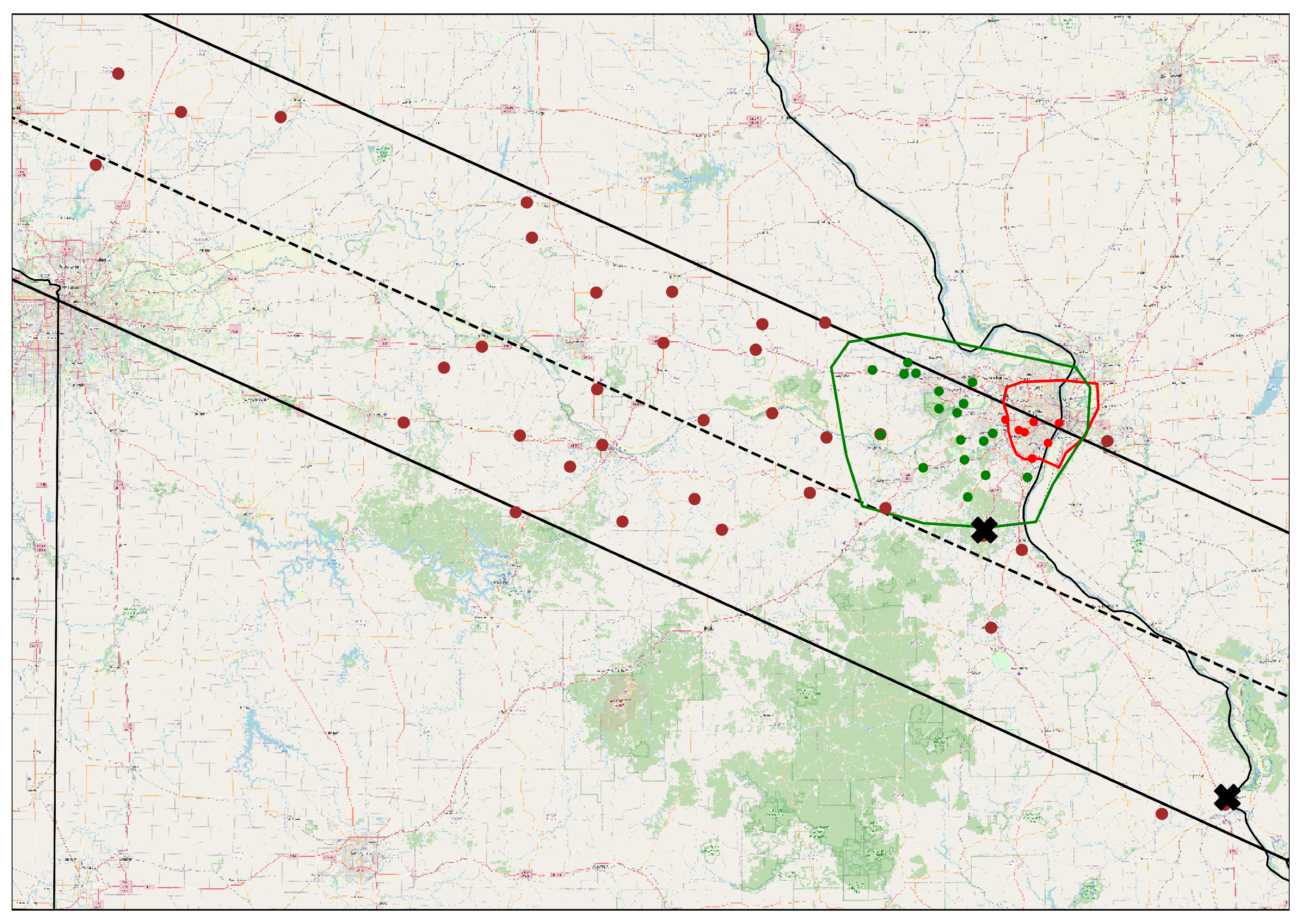
2.1. Surface Mesonet

The QuantumWeather^® meso meteorological network (QW), developed through a partnership between Saint Louis University and Ameren Missouri, is a permanent 80 station surface mesonet with a mixture of RainWise Mk-3 and Lufft WS600-umb sensor suites, and an upper air network of three InterMet sounding systems Figure 1.

The sounding systems used in this analysis were located on the Saint Louis University Campus, at Jefferson Community College (located on the center line of the eclipse) and at the Ameren-Missouri facility in Cape Girardeau.

Temperature, relative humidity, pressure, wind speed, wind direction, wind gust, precipitation, and solar panel voltage (a stand in for insolation) are recorded once a minute at each site. A comprehensive quality assurance/quality control (QA/QC) system is in place to complement the network’s efficient collection and transmission of environmental observations. The characteristics of mesonet sites are also generally consistent with standards recommended by the American Association of State Climatologists (AASC) for automated weather station networks.

As noted earlier, this network was used by Mainhart et al. [17] to study the Saint Louis urban heat island (UHI), and the high spatial and temporal resolution of the QuantumWeather^® network is well suited to study the effects of the eclipse on the atmosphere during the eclipse, as well as how the UHI formed by the city of Saint Louis altered the atmospheric response to the eclipse.

2.2. Quantum Weather^® Quality Control/Assurance

The need for thorough, rapid, and efficient collection, retrieval, and data archiving, combined with the need to optimize the daily performance of the network, dictated a multi-layered approach to the mesonet’s QA system:

• Assess the quality and correct for any known biases in a real-time basis so the mesonet data can be used to produce on-demand forecasts;
• Augment data archives with a trustworthy assessment of the confidence in each datum, create biases corrections as necessary; and
• Assess the ongoing performance of the network to keep current and future data quality at the highest level that is operationally possible.

QuantumWeather’s QA/QC process is similar to that used by the Oklahoma mesonet [20]. A sanity check is first applied to the data to capture instrument failures; to capture out of bounds values; and to apply bias corrections, which fix observations errors that are due to site changes over time (a tree grows tall enough to obstruct the wind for example). Temperature bias corrections are typically a degree or less, while relative humidity shows a 10% to 15% bias.

The time continuity or persistence tests check data from a single station across a 5-minute period. The change in the parameter value across that five minute period is then compared with a threshold value. If the parameter difference is larger than a defined standard deviation, the corresponding data values are flagged as ’suspect’.

The third QA check is a spatial continuity test. The spatial continuity test uses a multi-pass Barnes objective analysis [21,22,23] to compute an estimate of the value of a parameter at a station from the surrounding stations. Each station is removed in turn from the list of stations used to compute the spatial analysis. This spatial analysis is then used to compute a value at the location of the station removed. The difference between the parameter at the station from spatial analysis without the station included in the analysis and the actual station parameter is then used to flag the value at the station. The assumption is that variables like temperature, pressure, and relative humidity are spatially constrained and that significant changes in the spatial analysis because a station is removed are a cause for concern.

Data for the day of the eclipse were extracted from the QW database and QC’d using the methods described above. In addition, the data set was manually examined to ensure that the automatic QC/QA procedure did not retain poor quality data or delete high-quality data. Particular attention was given to data between 16UTC and 22UTC.

2.3. Methdology

Although a standard meteogram, such as Mahmood’s [6] Figure 4 would document the effects of the eclipse at that mesonet site, the effects of the suburban and urban environments would be overwhelmed by local site variations. Thus, local station siting effects need to be removed from the dataset. In this study, local effects were removed by compositing mesonet data along the eclipse path. Mesonet data were grouped into rural stations along the eclipse path well away from urban areas, those stations that are outside the urban area but not truly rural, and stations in the eclipse path in an urban area. Urban stations were defined as stations within the immediate Saint Louis city and county, suburban stations as stations within the Saint Louis metro area but outside the urban area, and rural stations as the remaining stations. In Figure 1, urban stations are those within the area encircled by the red line, suburban stations are those encircled by the green line but outside the red line, and all other stations are rural stations. The composite meteograms were constructed by computing the 1-minute mean and standard deviation of all the stations and of the rural, suburban, and urban stations only. These composite meteograms were plotted using the 5-minute means, and a polynomial fit created a smooth curve through the data. To provide context for the composite meteograms, meteograms for a single station in each domain are shown in Figure 2 below. Eclipse event timings for Western, Central, and Eastern Missouri are given in

Table 1. Eclipse event times for Western, Central, and Eastern Missouri.

	First Contact	Totality Start	Totality End	Last Contact
Western Missouri (Saint Joseph)	16:40:34	18:06:19	18:08:57	19:34:27
Central Missouri (Jefferson City)	16:46:05	18:13:08	18:15:35	19:41:04
Eastern Missouri (Cape Girardeau)	16:51:55	18:20:20	18:22:02	19:47:34

.

In addition to the composite meteograms, contour plots of temperature, relative humidity, pressure, and solar panel voltage were constructed at 5-minute intervals. A Barnes objective analysis [21,22,23] was used to grid the irregularly spaced station data to a regular grid with a grid spacing of 30 km. NCAR’s graphical contouring routines were used to plot the gridded data. As a consequence of QW’s design goals, the Saint Louis metro region has a higher station density than the rest of Missouri (Figure 1) compared to other parts of the state. The average station spacing in the rural domain is 60 km, while the urban domain average station spacing is 20 km. The objective analysis was configured to require a minimum of two points and a scan radius of 100 km. When examining the contoured plots, care needs to be taken near the edges of the contoured data as the objective analysis tends to exponentially extrapolate data near the edges of the contoured field. Care was taken to minimize these effects, but they cannot be eliminated.

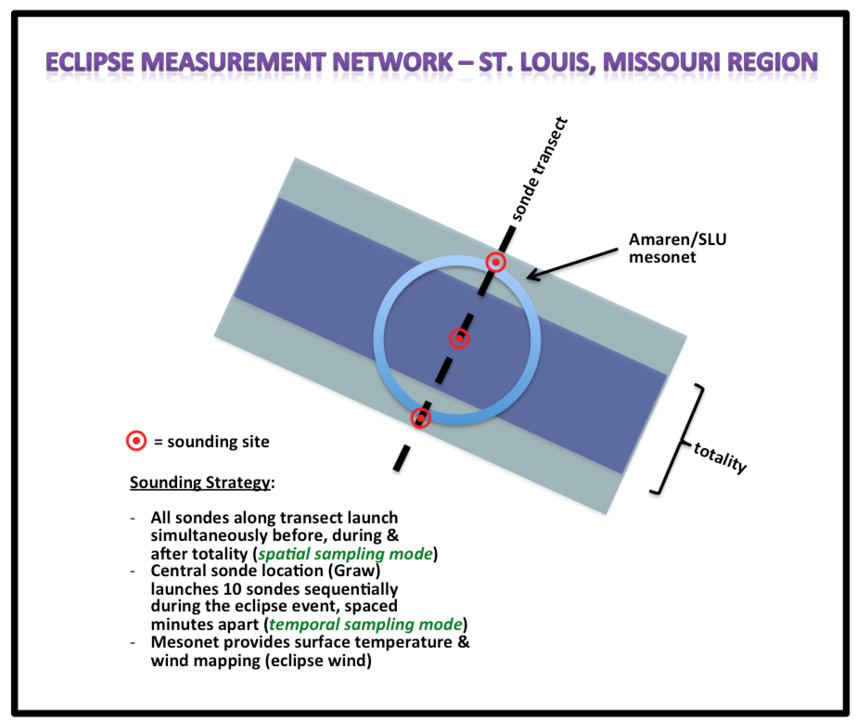
2.4. Radiosonde Observations

In addition to surface measurements, three InterMet Systems iMet-1 radiosonde systems were deployed to measure how the planetary boundary layer responded to the eclipse (Figure 3).

The northernmost site was located on Saint Louis University’s main campus, the central site at Jefferson Community College (JEFCO) in Hillsboro Missouri, and the southernmost site on the Ameren-Missouri facility in Cape Girardeau Missouri (CG). Coordinated launches measuring temperature, relative humidity, pressure, wind speed, and wind direction with a vertical resolution of about 10 m were made before, during, and after totality. Vertical profiles were constructed to determine the magnitude of the temperature drop and change in winds, if any, in the planetary boundary layer. The three sites also allowed planetary boundary layer variations across the eclipse path to be measured. A hardware failure at the Saint Louis University site prevented launches from that site; other launches were successfully conducted within minutes of the proposed launch schedule. The choice of termination altitude and of the radiosonde campaign was planned to focus on boundary layer measurements in accordance with the goals of the field campaign.

All of the sounding data were analyzed and QC’d using NCAR’s ASPEN (atmospheric sounding processing environment). ASPEN is designed to automatically apply quality control procedures to the sounding data while at the same time allowing users to tune the quality control algorithms to fit a particular sounding set [24]. ASPEN uses an extensive series of QC algorithms on the data set that may be adjusted by the user if the default values are not suitable for a particular sounding. In most cases, this first pass will be the only one required. The QC’d and QA’d sounding data were then plotted using the NCAR graphics Skew T plot routines. The automatic quality control values were sufficient to produce a clean sounding from all of the soundings collected during the eclipse.

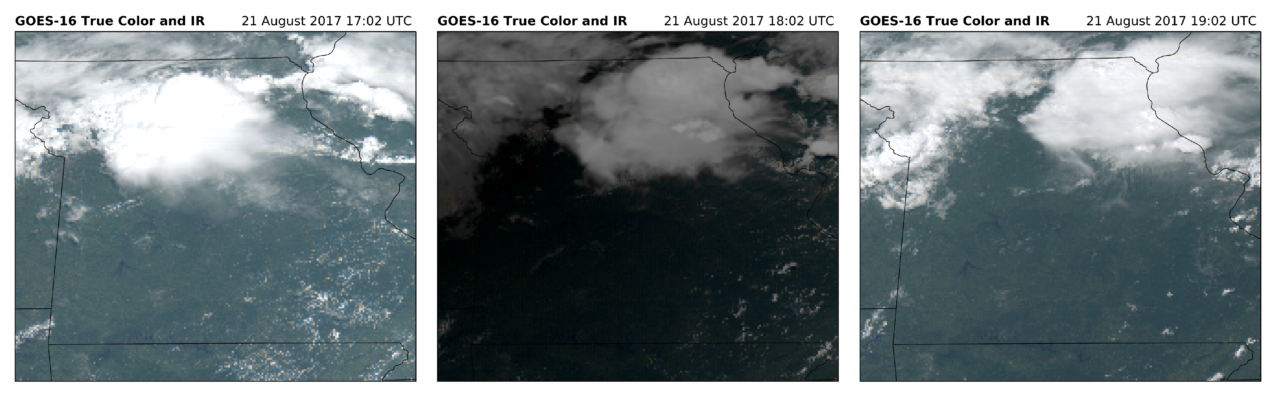
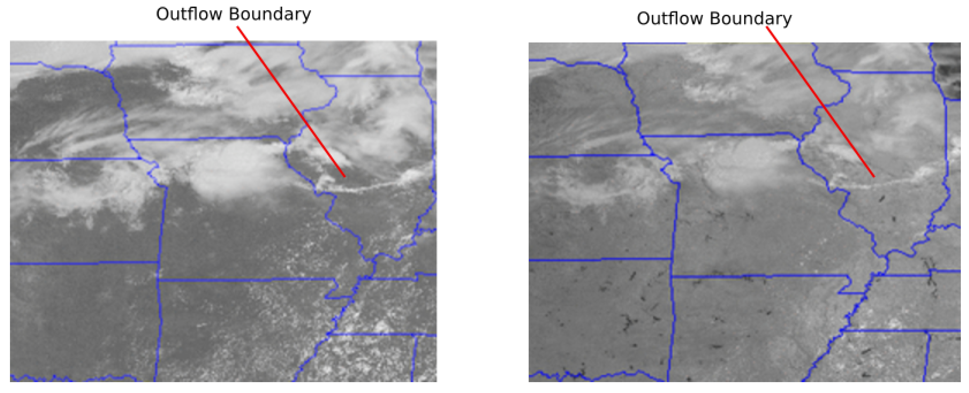
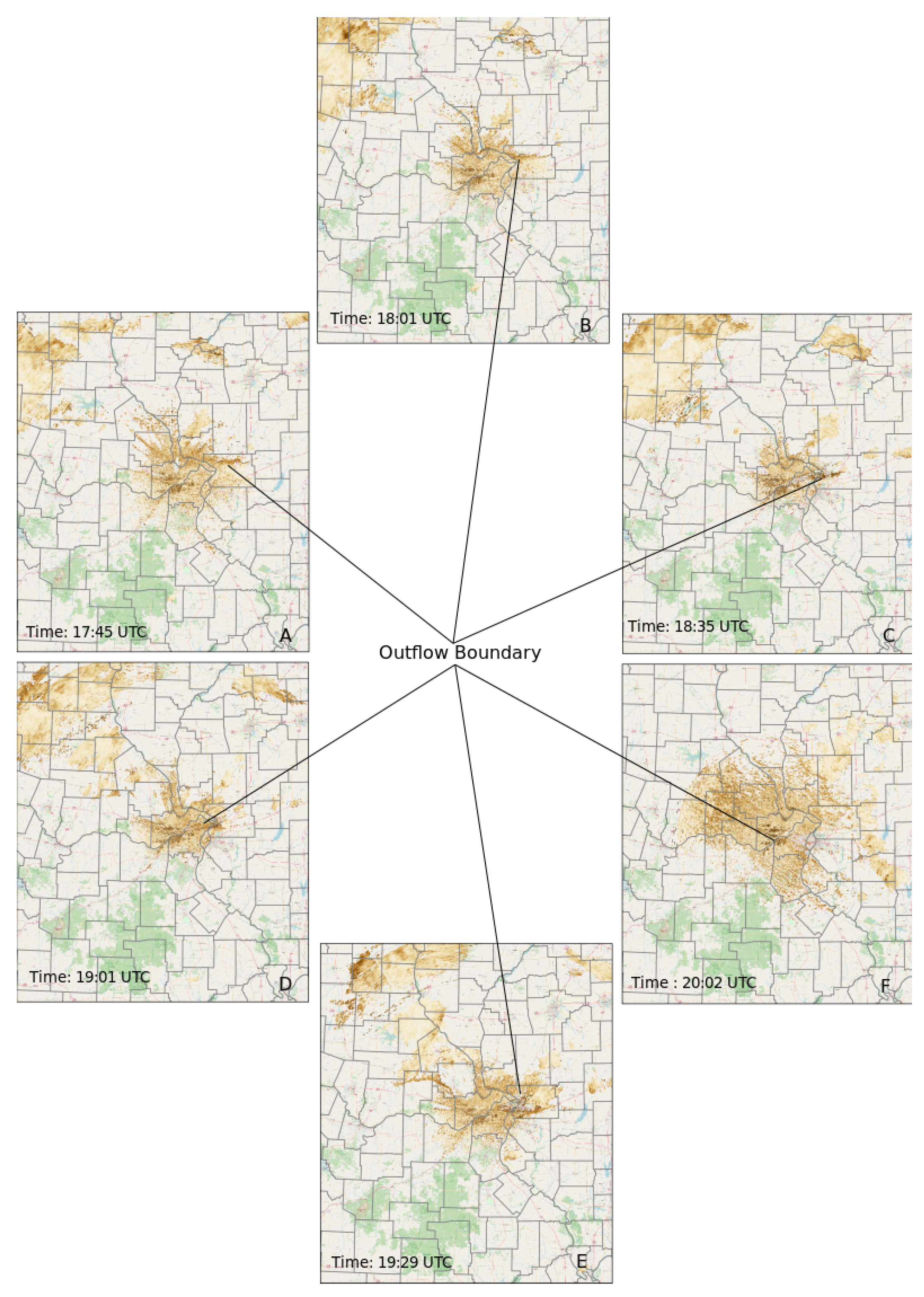
2.5. Assessing Contamination of Mesonet Data by Nearby Convective Complexes

Contoured real-time mesoanalysis (RTMA) temperatures for the hour before, the hour during, and the hour after the eclipse are presented in Figure 4. Although the RTMA temperature fields have a 2.5 km resolution, RTMA’s 12-minute data assimilation window minimizes the effects of the eclipse on the analyzed temperature field. The effects of the eclipse are only barely captured in the northwest corner of Missouri at 18:00 UTC. There, eclipse-generated cooling appears to combine with the cool pool (cold downdraft air) deposited by a band of storms that moved along the Missouri/Iowa border (Figure 4).

The cool pool remained along the northern tier of Missouri from 17:00–19:00 UTC and built further eastward into west-central Illinois. In the RTMA temperature imagery, the Saint Louis urban heat island was clearly seen to strengthen as the day progressed. The sequence of satellite imagery revealed the dense cirrostratus exhaust of the convective complex as it tracked toward the east. Note the pronounced darkening of visible satellite images around 18:00 UTC as the eclipse shadow crosses Missouri (Figure 5).

The RTMA wind analysis shows a moderate outflow boundary associated with the thunderstorms along the Missouri/Iowa border. Wind gusts of up to 14 ms⁻¹ are seen in the hour before the eclipse, but the gusts associated with the thunderstorms along the border decrease with time (Figure 6). By 20:00 UTC the strongest wind gusts were in northern Illinois. The National Weather Service hand analysis denoted a weak outflow boundary that appears in the Saint Louis 17:57 UTC, 18:35 UTC radar reflectivity (Figure 7) and does not appear in the 2.5 km RTMA wind or temperature fields.

The RTMA winds showed a distinct outflow boundary with gusts as high as 14 ms⁻¹ associated with the most intense parts of the thunderstorms in northwestern Missouri and along the Missouri/Iowa border. As the afternoon progressed, these outflows decreased. An outflow boundary seen in the reflectivity and spectrum width images (Figure 7) was not associated with these thunderstorms but with storms over the far western region of Illinois.

The boundary appears to have sagged slowly southward and by 18:16 universal time coordinated (UTC) was no longer apparent within the ground clutter field of the radar. Wind gusts in the Saint Louis in the Saint Louis metro area remained under 8 ms⁻¹ during the period, and the decaying gust front did not appear to perturb the background wind field.

3. Results

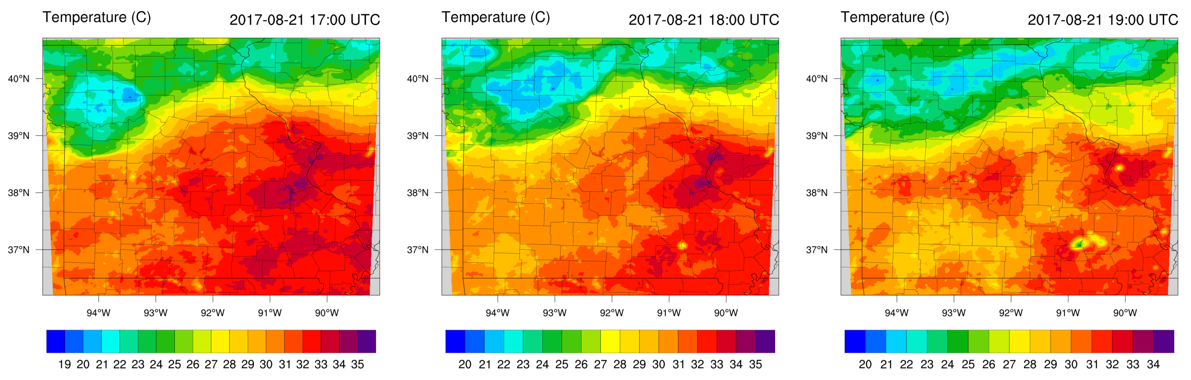
3.1. Domain Surface Temperature Response

The first order response of the surface and lower boundary layer to the eclipse was pronounced cooling. The magnitude and progression of the eclipse shadow across the greater St. Louis region is shown in the following Figure 8, which is a mosaic of panels constructed at 5-min intervals and based on the high-resolution surface network. We have chosen to zoom in on the region encompassing the greater St. Louis suburban zone and path of totality (solid, parallel lines with exact center line of totality also shown). Color contours indicate spatial temperature variations at 5-min intervals (18:10–18:35 UTC) and are rendered according to the color bar shown in the bottom center of the image. The inner solid polygon encompasses the St. Louis urban area proper; the outer polygon encompasses the suburban zone.

There are several features of note prior to the onset of totality in the St. Louis region (18:10 UTC). First and foremost is a zonal gradient with lower temperatures west of St. Louis and higher temperatures within the urban core. The urban–rural difference amounts to 4 °C in the zonal orientation. Given prevailing surface westerlies, some advection of the urban core’s heat dome was noted downwind or east of the city core proper. Second, as discussed in the previous section, a convective-generated cool pool lay to the north of St. Louis. At 18:10 UTC, this mass of lower temperature air (26 °C–27 °C) is pointed out by the arrow. Third, an area of lower temperatures appeared along the far western border of analyzed temperatures and is believed to be an artifact generated along the boundary by the Barnes objective analysis technique.

By 18:20 UTC, we note a west-to-east cooling trend of 1 °C to 2 °C commencing near the center of the zoomed panel and starting to impinge on the western portion of the St. Louis urban core. From 18:10 UTC to 18:25 UTC, the the temperature isolines are tightening, signaling that the urban heat island is moderating the temperature changes due to the eclipse. By 18:30 UTC, the urban core had reached maximum cooling as the centroid of the totality zone spread eastward. The urban center cooled 1 °C to 2 °C while a zone of more pronounced eclipse cooling, from 30 °C to 27 °C, developed in the rural region west of St. Louis.

At 18:30 UTC, a distinct temperature minimum of 4 °C on the center line of the eclipse path is observed. The time lag between minimum temperature realized at 18:30 UTC and temporal center point of the period of totality was approximately 14 min, comparable to that noted by Alpin [2]. At 18:35 UTC, with totality having concluded across the region, rapid recovery to pre-eclipse temperature values progressed across much of the domain.

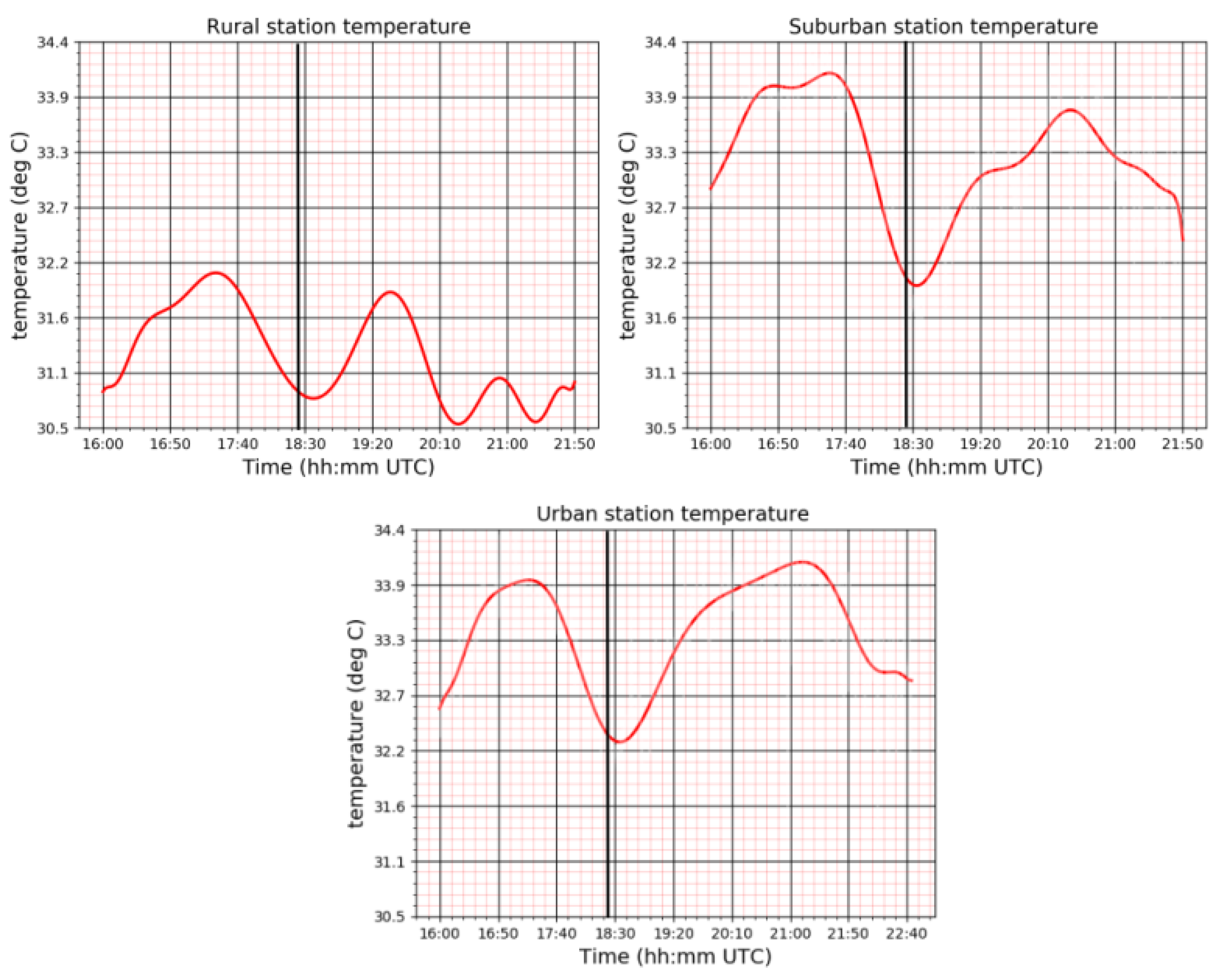
3.2. Time Series Response—Surface Temperature Sensors

Time series plots of surface immediately before, during, and after totality were generated using a compositing technique. The compositing technique classifies stations according to land use type, including rural, suburban, and urban core settings. Urban sites (Figure 1) were selected on the basis of being inside the urban core defined as Saint Louis city and Saint Louis county. Suburban sites included counties immediately surrounding St. Louis city and County that form the Saint Louis metropolitan area. All other sites were considered rural. Because of heterogeneities in land characteristics, it is important to look for differences in the thermal response to the sudden loss of radiative forcing during eclipse totality. For all of the three time series plots shown, a 15th order polynomial curve function fit to the station averaged 1-minute instantaneous data.

The three composite plots are shown below in Figure 9. In all of the plots, the red curves show a 15th-order polynomial fit to instantaneous (every 5 min) values. Peak totality is evident in all three of the sites by the sudden decrease in air temperature, and their rapid recovery At the start of the eclipse, surface sensors indicated higher temperatures in the urban regions (33.9 °C) than in the rural regions (32.7 °C). The magnitude of the drop during totality, interestingly, is similar for all three land uses ranging from 1.7 °C to 2.1 °C.

The temperature drop in all three settings was swift and sustained. The same cannot be said about the temperature recovery. For the composite of rural sites, the rate of temperature increase-post totality was initially rapid but then plateaued, oscillating for an hour and a half around a mean value of 32.2 °C, with final recovery back to 33.9 °C roughly 3.5 h post-totality. As shown in Mahmood’s Figure 4 [6], there are rapid fluctuations in the observed incoming solar radiation due to passing cumulus clouds (see Figure 5). These fluctuations in incoming solar radiation moderate the recovery of temperatures. The effect is most pronounced in the rural data and less pronounced in the urban data, likely the result of the UHI.

The composite suburban station’s temperature recovery was also quite extended, starting with a rapid rise and then much slower increase, and after 3.0 h peak recovery it fell short of the starting temperature by 0.4 °C. For the urban site composite, the recovery period was also protracted (2.5 h) but the post-eclipse temperature was identical to the pre-eclipse value. Again, the temperature recovery is likely moderated by the UHI.

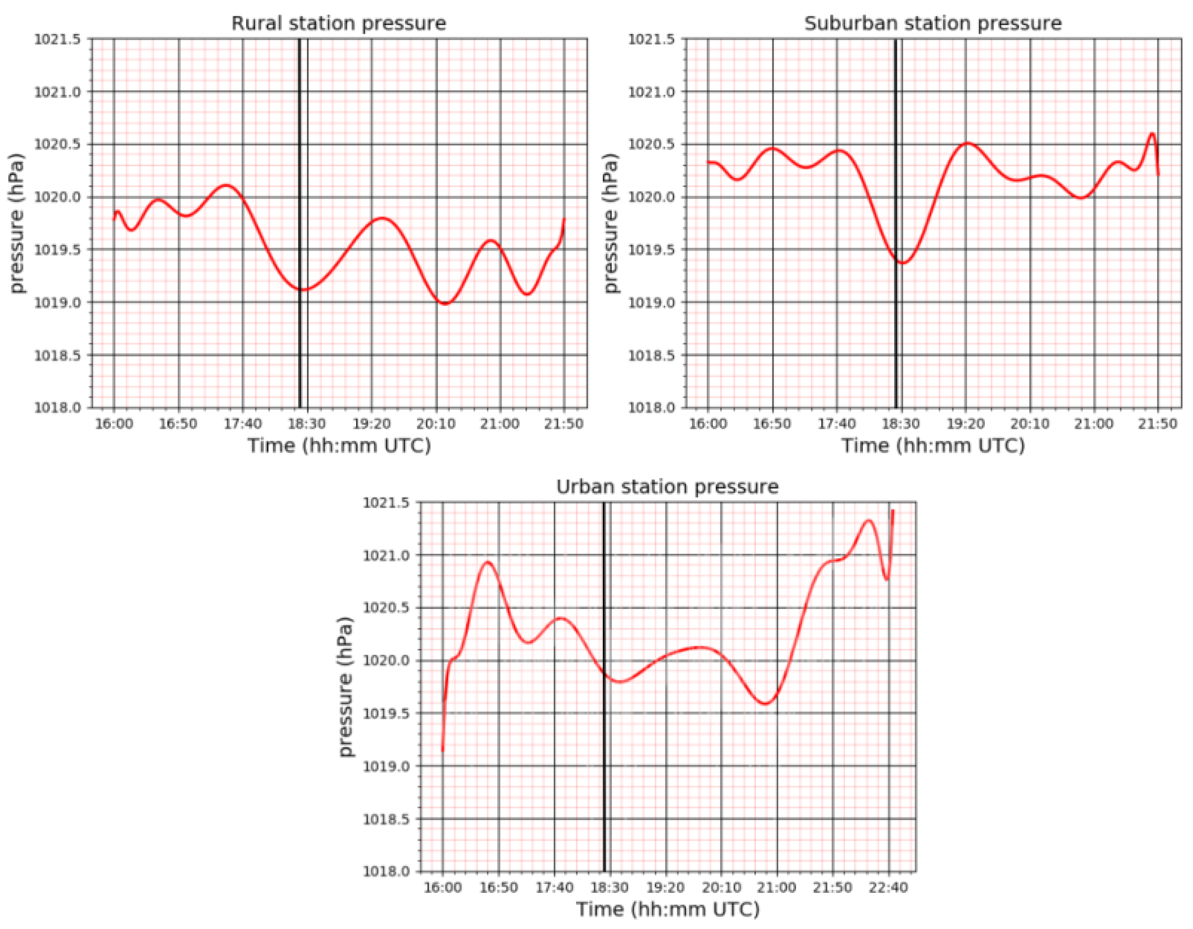
3.3. Time Series Response—Surface Pressure Sensors

The surface station pressure response is examined next (Figure 10). The pressure response at all three sites can best be described as a series of oscillations, of mixed periodicity, and of amplitude. In the composite of rural sites, there was the appearance of a damped oscillation, with the strongest amplitude approximately at the time of totality, just before the time of minimum temperature.

Contrary to what is noted in these plots, at the time of coolest surface temperature, air density should be maximized, requiring a transient pressure maximum. The complexity shown here suggests the need for an alternative explanation.

Pressure oscillations in the suburban and rural regions were of lower overall amplitude (1 hPa) and do not appear to have dampened with time. On the other hand, the urban pressure change was much larger (1.6 hPa), and showed a more complex oscillation pattern. This suggests that the greater preponderance of built and elevated structures such as buildings, tall bridges, and signs may collectively dampen some wave modes and excite others, especially as the flow becomes increasingly turbulent during these interactions.

As noted earlier, the composite pressure fields should have shown a pressure maximum at the time of maximum cooling; instead, the composite pressure fields displayed a pressure minimum at the time of the eclipse followed by a damped oscillation. One possible explanation is that the thermal and pressure fields were decoupled by a series of gravity waves propagating in the planetary boundary layer (PBL). Although eclipse-induced gravity waves at the continental scale in the ionosphere and mesosphere have been documented by Beer [25] and Nayak and Yigit [26], other explanations for the apparent wave motion at the mesoscale near the surface are possible. As noted earlier, the 17:45 UTC St Louis radar reflectivity showed a weak outflow boundary that was seen in the reflectivity fields as late as 20:10 UTC (Figure 7). The passage of a outflow boundary, created by the thunderstorms located well beyond the mesonet domain, propagated across the mesonet. This outflow boundary manifests its presence in the pressure field as a damped oscillation. The pressure oscillations may in part explain oscillations in surface temperature during the post-eclipse recovery period. Although this outflow boundary was not strong enough to appear in the reflectivity data as it continued to move southward, the outflow boundary can be seen in the spectrum width fields as late as 20:05 UTC. Further, GOES-16 rapid scan visual wavelength imagery from 17:22 UTC shows the presences of the outflow boundary. This damped oscillation is more evident in the rural pressure fields due to lack of obstructions to the flow (Figure 11).

This outflow boundary continued to manifest itself through the development of thunderstorms to the south and east of Saint Louis after 20:00 UTC.

Although eclipse-induced effects on temperature are well understood and documented, the effects on wind speed and direction are more controversial (Figure 12). As noted by Gray et al. [8], the air cools in response to the eclipse, and then as the shadow moves away, the air rapidly warms again. The temperature plots shown (Figure 8) above clearly demonstrate this effect.

However, this also means that the warm air stops rising, begins to descend, and then suddenly starts rising again. This rapid change in speed and direction is one hypothesized mechanism behind the eclipse wind. The station plots of wind speed show a clear change in speed as the eclipse shadow passes over and is aligned with the rapid drop in temperature. This drop in speed and then recovery can also be seen in the composite wind speed plots for rural suburban and urban environments (Figure 13). Although the rural stations show the rapid decline and slow recovery of wind speeds, the suburban and urban stations show oscillations in the wind speed, particularly in the suburban stations. Although individual stations show a rapid decrease in speed as the shadow passes, there is a significant difference between an individual station plot and the contoured wind speed plots (Figure 14). At all times during the period of totality, a distinct center of wind maximum is evident centered on the path of totality. Winds reported by the western most stations are increasing and are returning to pre-eclipse values, while the easternmost stations are decreasing in response to the shadow. Wind directions from individual stations show these direction changes.

3.4. Sounding Data

In contrast to the discussion of the changes in surface conditions as noted above, much less effort has been devoted to studying the responses of the planetary boundary layer (PBL). This is partially due to lack of upper-air observations with high spatial and temporal resolution that capture the short lifetime of the eclipse. Vertical profiles of temperature, pressure, wind speed, and wind direction provide an opportunity to observe how the vertical structure of the atmosphere is affected by a dramatic loss of insolation during the eclipse. Two approaches were taken with the soundings launched during the eclipse. The first approach was to allow the sondes to rise to near 400 hPa to observe changes that occur throughout the entire column before, during and after the eclipse.

This approach was used with the CG launch site. Located on the southern edge of totality, where the effect of the total eclipse was minimal, sondes were launched at 16:39 UTC, 18:15 UTC, and 19:07 UTC, providing vertical profiles of the pre-eclipse environment, the eclipse environment, and the environment immediately after the eclipse.

The second approach was to rapidly launch sondes and allow them to only rise to approximately 800 hPa. Limiting the rise to 800 hPa prevents one from observing the changes over the entire column, but increased the temporal resolution and permitted changes in the PBL to be observed. This approach was used at the Jefferson Community College (JEFCO) site located on the center line, where sondes were launched every 15 min. Problems with the 18:45 UTC sonde not activating prevented the launch of the last sonde at JEFCO. A map of the sounding sites is shown in Figure 1. Soundings from the CG and JEFCO sites are presented in Figure 15 and Figure 16 below.

The JEFCO sounding, Figure 15, clearly shows the effect of the cooling associated with the passage of the eclipse shadow. At the JEFCO launch site, the surface temperatures drop from 32.0 °C to 30.9 °C at the first level above the ground during the eclipse, while the temperatures above 980 hPa are nearly identical to the pre-eclipse temperatures (30.8 °C pre-eclipse 30.6 °C eclipse), indicating the limited effect of surface cooling on the vertical column. Both soundings show dry adiabatic ascent (surface based dry adiabat in black) once the sonde leaves the surface layer. The composite JEFCO sounding Figure 17 clearly shows the temperature difference between before and during the eclipse and also shows a clear moistening of the column. The shallowness of the eclipse cold pool is unexpected.

The CG soundings do not show a drop in temperatures but rather a small increase in the near surface temperature over the course of the roughly 2.5 h between the first and last sounding. This is consistent with warming between the late morning and early afternoon. Although the pre-eclipse sounding was slightly higher than the adiabatic lapse rates, the eclipse and post-eclipse soundings exhibited nearly dry adiabatic lapse rates. In the Cape composite sounding Figure 17, the vertical profile exhibits significant moistening of the column between the 16:09 UTC sounding and the 18:25 UTC and 19:07 UTC soundings. The smaller changes at the CG sounding site are inline with what would be expected from a site at the edge of the eclipse center line.

Although there have been measurements of boundary layer height using radiosondes during eclipses, few studies exist. During the 2006 eclipse over Greece, a change in the boundary layer of approximately 175 m was measured with radiosondes Amiridis et al. [27], while during the 2015 eclipse over the British Isles, authors Gray and Harrison [8] stated there was observational evidence of a boundary layer height change but their data were not shown. Palomaki et al. [12] observed similar low-level temperature decreases in observed valley wind changes during the 2017 solar eclipse, although in their study the changes in low-level temperatures were strongly affected by a gust front from a convective cell 15 km away that past across the network. The rapid low-level radiosonde launched from the JEFCO site shows the rapid cooling in the lowest few hundred meters, resulting in a strengthening of the low-level inversion followed by a dry adiabatic ascent, indicating a significant change in the PBL height.

In this study, two methods were used to determine the height of the PBL. The first was used to calculate the PBL height using the Richardson method (Seidel [28]).

$$R_i=\frac{\frac{g}{{\theta }_v}({\theta }_{vz}-{\theta }_{vs})(z-z_s)}{{(u-u_s)}^2+{(v-v_s)}^2+b{u_{*}}^2}$$

where z is height and s denotes the surface, g is the acceleration of gravity, ${\theta }_v$ is virtual potential temperature (excluding condensate loading), u and v are the component wind speeds, b is a constant, and $u_{*}$ is the surface friction velocity. Since $u_{*}$ is not known from radiosonde data, b was set to 0.

The computed values were compared to PBL heights estimated by inspecting the dew point and temperature profile for the presence of a PBL capping inversion.

At the JEFCO sounding point, the Richardson method shows a 15 hPa change and a 20 hPa change via the capping method

Table 2. Jefferson Community College and Cape Girardeau PBL heights via capping method and computed using the Richardson method.

Jefferson Community College
Time	Richardson	Capping
18:13 UTC	861 hPa	858 hPa
18:27 UTC	834 hPa	848 hPa
Cape Girardeau
Time	Richardson	Capping
16:39 UTC	861 mb	858 mb
18:13 UTC	878 mb	880 mb
19:07 UTC	873 mb	878 mb

. The CG sounding shows a similar but smaller change consistent with its location further from the centerline of the eclipse Table 2. The PBL heights from the soundings match well with PBL height changes observed by Mahmood [6]. Differences in PBL height between those observed at the CG and JEFCO sites and those observed by Mahmood [6] are accounted for by the 1 min sample time of the Doppler LIDAR and the much longer sample time of the radiosondes. We suspect the collapse of the PBL is directly related to the loss of daytime heating and the resultant reduction in convective turbulence. Amiridis et al. [27] found a similar drop and recovery in PBL heights when radiosonde data were assimilated into the comprehensive air quality model with extensions (CAMQx).

In addition to the changes in PBL height, the JEFCO and CG soundings also show significant increases in convective available potential energy (CAPE) and decreases in CIN and LCL during the eclipse, indicating a significant change in water vapor content (Table 2 and

Table 3. Jefferson Community College and Cape Girardeau thermodynamic parameters.

Jefferson Community College
Time	LCL	CAPE	CIN
18:13 UTC	894 hPa	13.8 J/Kg	−32.9 J/Kg
18:27 UTC	920 hPa	43.2 J/Kg	−23.7 J/Kg
Cape Girardeau
Time	LCL	CAPE	CIN
16:09 UTC	912 hPa	811.6 J Kg	−12.3 J Kg
18:15 UTC	947 hPa	1661.3 J kG	−0.03J Kg
19:07 UTC	949 hPa	1834.5 J Kg	0.0 J Kg

). Mahmood et al. [6] noted a similar increase in radiometer measured water vapor content. The temperatures below the capping inversion shift from slightly stable before the eclipse to neutral during the eclipse and then back to slightly stable after the eclipse, supporting the increase in water vapor content.

Although the CG sounding plot shows a significant change in the wind speeds below 750 hPa, the differences are actually small and the result of how the wind barbs were plotted. The 17:45 UTC wind speeds are between 3.8 and 7.7 ms⁻¹, while the wind speeds for the 18:15 UTC and 18:48 UTC soundings were between 9.7 and 13.6 ms⁻¹. While there was only a small change in the wind speeds, the wind directions in the lowest 850 hPa changed significantly from a southerly to south-westerly direction.The JEFCO sounding shows a similar shift from westerly to southwesterly.

As discussed earlier, the observed oscillations in the pressure field could be explained by the passage of an outflow boundary. It is well known that thunderstorm-induced cool pools may contain one or more surges. This interpretation is supported by sounding data. The JEFCO and CG sounding sites show a significant increase in the dew point temperatures, an increase in CAPE, and a lowering of LCL, followed by a recovery. Given the slow movement of the outflow boundary and the distance between the JEFCO and CG sounding sites, the pressure oscillation and some of the boundary layer moistening could be explained by the passage of the outflow boundary. Unfortunately, the way the sounding data were collected did not allow for the capture of a complete sampling of the outflow boundary passage, so a definitive answer is not possible.

4. Summary

A region of eclipse-induced cooling was noted to propagate along the totality path, cooling the air by approximately 3 °C. Prior to the eclipse, the spatial analysis indicated an UHI centered on the St. Louis metro region with temperatures 3 °C (33.5 °C–30.5 °C) higher than the surrounding environs. The tightening of temperature contours signals that the urban heat island is modifying the temperature changes due to the eclipse. As the eclipse cooled air passed across the UHI, temperatures in the UHI were reduced by 2 °C. The maximum eclipsed induced cooling occurred approximately 14 min after the actual passage of the eclipse shadow. The observed delay in cooling is in line with previous studies, as noted above.

The composite time series analyses were constructed for all the temperature responses. The rural, suburban, and urban composites indicated a swift drop in surface temperature of 1.7 °C (urban core), 2.0 °C (suburban), and 2.1 °C (rural) as totality approached. The time series analyses show that for all three composites, the recovery of surface temperature under strong, mid-afternoon sun post-eclipse was delayed by up to 2–3 h and tended to oscillate during recovery. The effects of the eclipsed-induced cooling were moderated by the UHI, with cooling in the urban core more strongly moderated than in the suburban areas. The short duration of the eclipse cooling and larger thermal mass of the urban core reduced the magnitude of the temperature drop.

The pressure response in the time series analysis shows a complex response. For all the pressure responses, the rural, suburban, and urban composites indicated a drop in surface pressures of between 0.8 hPa and 1.6 hPa during the maximum eclipse followed by a series of wavelike pulses, of varying amplitude and frequency, with the pressure minimum coinciding with the time of peak cooling. This, at first, would seem paradoxical as cooler surface air should thermodynamically favor a transient density increase and hence pressure maximum. Rather than an internal gravity wave, this transitory signal in the pressure field is consistent with the passage of an outflow boundary created by thunderstorms located beyond the mesonet domain that propagated across the mesonet. The pressure oscillations may in part explain oscillations in surface temperature during the post-eclipse recovery period as outflow surges behind the gust front passed through the mesonet work.

The winds during the day of the eclipse were weak under the influence of a surface high pressure. These weak surface winds resulted in large variations in speed and direction, as shown by the individual station locations, (Figure 2). As expected, wind speeds in the rural and suburban areas were higher than in the urban core. Surface winds across the domain revealed a localized wind maximum along the center of totality, which tended to persist west of the St. Louis urban region. As the eclipse shadow moved eastward into the Saint Louis metropolitan area, the increased urbanization disrupted the wind sufficiently to remove the signal from the data.

Two series of soundings obtained, one near the outer edge of totality and the other close to the eclipse center line, document the small effects of the eclipse on the vertical structure of the atmosphere. Although both sites show moistening of the vertical profile near the surface, only the JEFCO site on the center line reveals a shallow eclipse-induced cold pool in the lowest 20 hPa. There are also significant changes to the dry adiabatic lapse rate in the boundary layer temperature and moistening of the dew point profile, particularly above 870 hPa. The Cape site shows typical temperature increases due to daytime heating and significant moistening of the vertical column. The soundings provide additional documentation for the effects of the passage of the outflow boundary. Although the changes in dew point temperatures, CAPE, and LCL height cannot be definitely ascribed to the passage of the outflow boundary, it is a viable explanation.

5. Conclusions

In this paper, we have presented a novel set of observations and analyses pertaining to a total solar eclipse across a portion of the U.S. Midwest on 21 August 2017. The focus of our effort has been to collect high-quality and high spatial and temporal measurements at the surface and in the boundary layer to assess spatial and temporal variations of atmospheric properties across the St. Louis greater metropolitan region and surrounding countryside.

Novel aspects of this study include (1) using a dense surface network to sample the eclipse response along portions of the path of totality; (2) examining how portions of inhomogeneous landscape (rural, suburban, and urban) differ in their response to eclipse passage; and (3) documenting the confounding influence of a thunderstorm outflow that passed through the network at the time of totality.

Our high spatial and temporal analysis of the temperature, pressure, and wind speed fields in rural areas show similar results to those shown previous studies. The response in the UHI demonstrates that the eclipsed induced cooling was moderated by the UHI, with cooling in the urban core more strongly moderated than in suburban areas. We believe the short duration of the eclipse cooling and the larger thermal mass of the urban core reduced the magnitude of the temperature drop.

The results of the sounding analysis document the very localized effect the eclipse had on the vertical structure of the eclipse. Only the JEFCO sounding site showed significant vertical temperature changes, and those changes were limited to the first 20 hPa. Furthermore, away from the center line of the eclipse changes in the vertical temperature were nearly non-existent. The unique combination of eclipse-induced changes and the thunderstorm outflow complicated the sounding analysis. Unfortunately, this complicated interaction was unanticipated in the original experiment design, and definitive answers about this interaction are not possible.

References

1. Clayton, H.H.; Rotch, A.L.; Pickering, E.C. The eclipse cyclone and the diurnal cyclones. In Annals of the Astronomical Observatory of Harvard College; The Observatory: Cambridge, UK, 1901. [Google Scholar]
2. Aplin, K.L.; Scott, C.J.; Gray, S.L. Atmospheric changes from solar eclipses. Philos. Trans. R. Soc. Math. Phys. Eng. Sci. 2016, 374, 20150217. [Google Scholar] [CrossRef] [PubMed]
3. Ahrens, D.; Iziomon, M.G.; Jaeger, L.; Matzarakis, A.; Mayer, H. Impacts of the solar eclipse of 11 August 1999 on routinely recorded meteorological and air quality data in south-west Germany. Meteorol. Z. 2001, 10, 215. [Google Scholar] [CrossRef]
4. Hanna, E. Meteorological effects of the solar eclipse of 11 August 1999. Weather 2000, 55, 430–446. [Google Scholar] [CrossRef]
5. Founda, D.; Melas, D.; Lykoudis, S.; Lisaridis, I.; Gerasopoulos, E.; Kouvarakis, G.; Petrakis, M.; Zerefos, C. The effect of the total solar eclipse of 29 March 2006 on meteorological variables in Greece. Atmos. Chem. Phys. 2007, 7, 5543–5553. [Google Scholar] [CrossRef]
6. Mahmood, R.; Schargorodski, M.; Rappin, E.; Griffin, M.; Collins, P.; Knupp, K.; Quilligan, A.; Wade, R.; Cary, K. The total solar eclipse of 2017: Meteorological observations from a statewide mesonet and atmospheric profiling systems. Bull. Am. Meteorol. Soc. 2020, 101, E720–E737. [Google Scholar] [CrossRef]
7. Turner, D.D.; Wulfmeyer, V.; Behrendt, A.; Bonin, T.A.; Choukulkar, A.; Newsom, R.K.; Brewer, W.A.; Cook, D.R. Response of the land-atmosphere system over north-central Oklahoma during the 2017 eclipse. Geophys. Res. Lett. 2018, 45, 1668–1675. [Google Scholar] [CrossRef]
8. Gray, S.L.; Harrison, R.G. Eclipse induced wind changes over the British Isles on the 20 March 2015. Philos. Trans. R. Soc. A Math. Phys. Eng. Sci. 2016, 374, 20150224. [Google Scholar] [CrossRef]
9. Burt, S. Meteorological responses in the atmospheric boundary layer over southern England to the deep partial eclipse of 20 March 2015. Philos. Trans. R. Soc. A Math. Phys. Eng. Sci. 2016, 374, 20150214. [Google Scholar] [CrossRef]
10. Fowler, J.; Wang, J.; Ross, D.; Colligan, T.; Godfrey, J. Measuring ARTSE2017: Results from Wyoming and New York. Bull. Am. Meteorol. Soc. 2019, 100, 1049–1060. [Google Scholar] [CrossRef]
11. Colligan, T.; Fowler, J.; Godfrey, J.; Spangrude, C. Detection of stratospheric gravity waves induced by the total solar eclipse of July 2, 2019. Sci. Rep. 2020, 10, 19428. [Google Scholar] [CrossRef]
12. Palomaki, R.T.; Babić, N.; Duine, G.J.; van den Bossche, M.; De Wekker, S.F. Observations of Thermally-Driven Winds in a Small Valley during the 21 August 2017 Solar Eclipse. Atmosphere 2019, 10, 389. [Google Scholar] [CrossRef]
13. Harrison, R.G.; Marlton, G.J.; Williams, P.D.; Nicoll, K.A. Coordinated weather balloon solar radiation measurements during a solar eclipse. Philos. Trans. R. Soc. A Math. Phys. Eng. Sci. 2016, 374, 20150221. [Google Scholar] [CrossRef] [PubMed]
14. Mazzarella, A.; Scafetta, N. Estimating Naples’ urban heat island effects using the March 20, 2015 partial solar eclipse. Cse-City Saf. Energy 2017, 63–69. [Google Scholar] [CrossRef]
15. Vukovich, F.M.; King, W.J. A theoretical study of the St. Louis heat island: Comparisons between observed data and simulation results on the urban heat island circulation. J. Appl. Meteorol. 1980, 19, 761–770. [Google Scholar] [CrossRef]
16. Fishman, J.; Belina, K.M.; Encarnación, C.H. The St. Louis ozone gardens: Visualizing the impact of a changing atmosphere. Bull. Am. Meteorol. Soc. 2014, 95, 1171–1176. [Google Scholar] [CrossRef]
17. Mainhart, M.; Pasken, R.; Chiao, S.; Roark, M. Surface mesovortices in relation to the urban heat island effect over the Saint Louis metropolitan area. Urban Clim. 2020, 31, 100580. [Google Scholar] [CrossRef]
18. Goodwin, G.L.; Hobson, G.J. Atmospheric gravity waves generated during a solar eclipse. Nature 1978, 275, 109–111. [Google Scholar] [CrossRef]
19. Buban, M.S.; Lee, T.R.; Dumas, E.J.; Baker, C.B.; Heuer, M. Observations and Numerical Simulation of the Effects of the 21 August 2017 North American Total Solar Eclipse on Surface Conditions and Atmospheric Boundary-Layer Evolution. Bound.-Layer Meteorol. 2019, 171, 257–270. [Google Scholar] [CrossRef]
20. Shafer, M.A.; Fiebrich, C.A.; Arndt, D.S.; Fredrickson, S.E.; Hughes, T.W. Quality assurance procedures in the Oklahoma Mesonetwork. J. Atmos. Ocean. Technol. 2000, 17, 474–494. [Google Scholar] [CrossRef]
21. Barnes, S.L. Applications of the Barnes objective analysis scheme. Part I: Effects of undersampling, wave position, and station randomness. J. Atmos. Ocean. Technol. 1994, 11, 1433–1448. [Google Scholar] [CrossRef]
22. Barnes, S.L. Applications of the Barnes objective analysis scheme. Part II: Improving derivative estimates. J. Atmos. Ocean. Technol. 1995, 11, 1449–1458. [Google Scholar] [CrossRef]
23. Barnes, S.L. Applications of the Barnes objective analysis scheme. Applications of the Barnes Objective Analysis Scheme. Part III: Tuning for Minimum Error. J. Atmos. Ocean. Technol. 1995, 11, 1449–1479. [Google Scholar] [CrossRef]
24. Martin, C.; Suhr, I. NCAR/EOL Atmospheric Sounding Processing ENvironment (ASPEN) Software. Version 3.4.5. 2021. Available online: https://www.eol.ucar.edu/content/aspen (accessed on 1 June 2022).
25. Beer, T. Supersonic Generation of Atmospheric Waves. Nature 1973, 242, 34. [Google Scholar] [CrossRef]
26. Nayak, C.; Yiğit, E. GPS-TEC observation of gravity waves generated in the ionosphere during 21 August 2017 total solar eclipse. J. Geophys. Res. Space Phys. 2018, 123, 725–738. [Google Scholar] [CrossRef]
27. Amiridis, V.; Melas, D.; Balis, D.S.; Papayannis, A.; Founda, D.; Katragkou, E.; Giannakaki, E.; Mamouri, R.E.; Gerasopoulos, E.; Zerefos, C. Aerosol Lidar observations and model calculations of the Planetary Boundary Layer evolution over Greece, during the March 2006 Total Solar Eclipse. Atmos. Chem. Phys. 2007, 7, 6181–6189. [Google Scholar] [CrossRef]
28. Seidel, D.J.; Zhang, Y.; Beljaars, A.; Golaz, J.; Jacobson, A.R.; Medeiros, B. Climatology of the planetary boundary layer over the continental United States and Europe. J. Geophys. Res. Atmos. 2012, 117, D17106. [Google Scholar] [CrossRef]
Figure 1. QuantumWeather® MesonetStation locations. Northern and southern eclipse bounds are in black. Center line is in dashed black. Urba bounds are in red, and suburban bounds are in green. Rural stations are in brown, suburban stations are in green, and urban stations are in red. Radiosonde sites are marked with a black x.
Atmosphere 14 01412 g001
Figure 2. Meteograms for rural (WS844 left), suburban (WS198 center), and urban (WS034 right) stations. Temperature, pressure, and solar panel voltage are in the top row. Wind speed and direction are in the bottom row. Solid lines are a 15th order polynomial fit to the data and the dashed lines are five minute samples.
Atmosphere 14 01412 g002
Figure 3. Radiosonde siting configuration.
Atmosphere 14 01412 g003
Figure 4. RTMA contoured temperature plots for 17:00 UTC, 18:00 UTC, and 19:00 UTC.
Atmosphere 14 01412 g004
Figure 5. Missouri-wide true-color satellite imagery for 17:02 UTC (left), 18:02 UTC (center), and 19:02 UTC (right).
Atmosphere 14 01412 g005
Figure 6. RTMA wind field for 17:00 UTC (left), 18:00 UTC (center), and 19:00 UTC (right).
Atmosphere 14 01412 g006
Figure 7. Saint Louis radar reflectivity and spectrum width for 17:45 UTC (left), 18:35 UTC (center), and 18:55 UTC (right).
Atmosphere 14 01412 g007
Figure 8. Mesonet-derived temperature (°C) fields for 18:10 (A), 18:15 (B), 18:20 (C), 18:25 (D), 18:30 (E), and 18:35 (F) UTC.
Atmosphere 14 01412 g008
Figure 9. Time history of temperature (°C) for rural, suburban, and urban sub-domains. Thick vertical thick black lines in the temperature plots represent the time of the eclipse.
Atmosphere 14 01412 g009
Figure 10. Time history of pressure for rural, suburban, and urban sub-domains. Thick vertical black lines in the pressure plots are the times of the eclipse.
Atmosphere 14 01412 g010
Figure 11. GOES-16 visual left and near-IR (0.86 microns) right imagery from 17:22 UTC.
Atmosphere 14 01412 g011
Figure 12. KLSX Spectrum Widths for 17:45 UTC (A), 18:01 UTC (B), 18:35 UTC (C), 19:01 UTC (D), 19:35 UTC (E), and 20:02 UTC (F).
Atmosphere 14 01412 g012
Figure 13. Mesonet-derived wind speed plots (ms−1) for 18:10 UTC (A), 18:15 UTC (B), 18:20 UTC (C), 18:25 UTC (D), 18:30 UTC (E), and 18:35 UTC (F).
Atmosphere 14 01412 g013
Figure 14. Time history of composite wind speed plots for rural, suburban, and urban sub-domains. Thick vertical black lines in the pressure plots are the times of the eclipse.
Atmosphere 14 01412 g014
Figure 15. SkewT plots from the Jefferson Community College (JEFCO) site for 18:13 UTC (left) and 18:26 UTC (right). Temperature trace in red, Dew Point temperatures trace in green, surface dry adiabat in black, and CAPE shaded in red. LCL marked with a black dot.
Atmosphere 14 01412 g015
Figure 16. SkewT plots from the Cape Girardeau (Cape) site at 16:39 UTC (left), 18:13 UTC (center), and 19:07 UTC (right). Temperature trace in red, Dew Point temperatures trace in green, surface dry adiabat in black, and CAPE shaded in red. LCL marked with a black dot.
Atmosphere 14 01412 g016
Figure 17. Composite JEFCO and Cape soundings. Solid lines are temperature and dashed lines are dewpoint temperatures.
Atmosphere 14 01412 g017