1. Introduction
Measurements of temperature, humidity, and wind in the boundary layer are sparse, although they are important for the initialization of numerical weather prediction models [
1]. In particular, the prediction of fog and winds could profit from additional measurements in the boundary layer [
2,
3,
4]. MeteoSwiss operationally assimilates atmospheric profiles from the following measuring instruments into its numerical weather prediction model COSMO (Consortium for Small-scale Modelling): radiosounding, radar and LiDAR wind profilers, microwave radiometers, and aircraft-derived observations (AMDAR and Mode-S).
Uncrewed Aircraft Systems (UAS) or drones are often presented as an opportunity to fill the observational gap in the boundary layer [
5,
6,
7,
8,
9,
10,
11]. The World Meteorological Organization recognized the potential of drones and will organize a demonstration campaign in 2024 [
12,
13]. There are several studies evaluating the performances of UAS for case studies or research applications. For example, Meteodrones were evaluated in detail by Inoue et al. [
14] with an analysis focused on seven profiles. Koch et al. [
15] analyzed the performances of the Meteodrone-SSE with respect to the balloon data for 37 flights over 5 days. The NOAA performed 241 Meteodrone-SEE flights over 5 months [
16,
17]. To the authors’ knowledge, the evaluation of the measurements has not yet been published. The performance of the CopterSonde was intensively studied over 141 flights with the analysis focused on 7 days, mostly during the LAPSE-RATE campaign [
11,
18,
19,
20]. In a recent analysis, Bärfuss et al. [
21] showed the performance of the LUCA UAS up to 10 km for six vertical profiles. Barbieri et al. [
22] analyzed the performances of 38 UAS with a comparison focused on 3 days of measurements. Muñoz et al. [
23] compared the performance of 10 UAS profiles with radiosondes, satellites, and numerical models. Laitinen et al. [
24] compared drone measurements with radiosondes and remote sensing instruments for 10 profiles. DataHawk has been extensively used [
25] and evaluated [
26], but this fixed-wing UAS is not optimized for unattended measurements. To the best of our knowledge, the operational capabilities of drones, i.e., their capability to operate unattended and continuously, have not yet been sufficiently evaluated. Moreover, there are still open issues regarding data quality, like heat exhaust from the drone [
27] or the position of the sensors [
28,
29,
30].
To better understand the maturity and the data quality of meteorological drones, MeteoSwiss, together with Meteomatics, conducted a proof-of-concept campaign, which included the long-term operation of a fully automated meteorological drone in Payerne, Switzerland. The main goal of this campaign was to evaluate the system and data availability, as well as the data quality.
This study focuses on data availability first, followed by two case studies. The last section investigates the quality of the Meteodrone measurements compared to sounding and remote sensing instruments.
2. Materials and Methods
2.1. Meteodrone
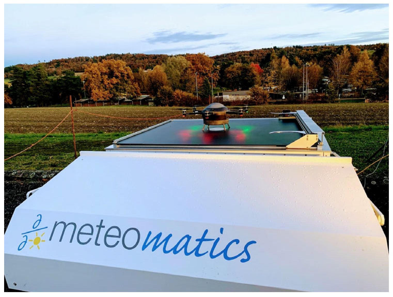
The Meteodrone MM-670 (
Figure 1) is a hexacopter designed and manufactured by Meteomatics [
10,
31]. The Meteodrone is designed to operate up to a maximum altitude of 6000 m, for wind speeds up to 25 m.s
−1 (90 km.h
−1), and for temperatures down to −50 °C. It is equipped with a parachute in case of emergency. The propellers are heated to be able to fly in icing conditions. The drone has a total weight of 5 kg and measures 70 cm in diameter.
The Meteobase is an automated shelter used to control the drone remotely and to recharge and protect the drone when it is not in use. A heating system kept this base above ambient temperature. The drone was programmed to perform and repeat customized flight patterns fully automatically. For safety reasons, it was mandatory for drone operations to always be supervised by a remote pilot. A “Specific Operations Risk Assessment” was required to obtain clearance from the Federal Office of Civil Aviation (FOCA). One of the safety rules was to call the air traffic controller every night to ensure no air traffic was planned around the drone. The base was equipped with a FLARM system on the ground to avoid potential collisions. The operations were also declared on the Daily Airspace Bulletin in Switzerland (DABS) to warn pilots and drone operators. From April to May, another restriction was added by the FOCA: flight operations were prohibited for wind directions between 315 and 45° to minimize the risk of the drone coming down on the Payerne camping area in the case of an incident.
For this campaign, the strategy was to fly at least eight times per 24 h during the working days. Due to aeronautical restrictions, it was not possible to fly during the daytime, so the flights were scheduled every hour from 20:00 to 04:00 UTC. To avoid interferences with the radiosonde launched at 23:00 UTC, the corresponding Meteodrone flight was scheduled for 23:15 UTC. The flights were planned to go up to 2000 m a.s.l. (around 1500 m a.g.l.). The Meteodrone MM-670 was equipped with one temperature sensor, two humidity and temperature sensors, and one pressure sensor [
14]. The type of the sensors remains confidential upon request from Meteomatics. The wind speed and direction were derived from the power of the six engines necessary to maintain its horizontal position.
This study assesses the manufacturer’s final data product, which was available in real-time from the drone system. The data were averaged on the way up and down, but the details of the data processing (time lag correction, averaging between the sensors, etc.) were not made available by Meteomatics, referring to the manufacturing intellectual property.
2.2. Sounding
Radiosoundings have been operated by MeteoSwiss at Payerne since 1942 [
32]. Soundings are launched twice a day at 11:00 and 23:00 UTC. Since 2018, the sondes have been type RS41 manufactured by Vaisala [
33]. Each radiosonde is automatically controlled before the sounding. The soundings are launched manually during office hours (typically weekdays during the daytime) and automatically the rest of the time. The typical maximum altitude is above 30 km [
34].
2.3. Remote Sensing
Payerne is a WMO “Measurement Lead Center” equipped with several remote sensing instruments [
35]. To contextualize the performance of the Meteodrones, this study aimed to compare the Meteodrone measurements to state-of-the-art remote sensing instruments.
At Payerne, the wind is measured at high temporal and spatial resolution with a Doppler LiDAR WLS-200 [
36] manufactured by Leosphere (Vaisala Group). It is a scanning LiDAR measuring around 1500 nm with a resolution of 50 m. The wind is calculated using the Doppler Beam Switching (DBS) technique with an independent wind profile every 15 s and an update rate of 3 s. In its operational configuration, the measurement range reaches from 100 m above ground to the top of the boundary layer. A radar wind profiler PCL1300 manufactured by Degreane also measures wind profiles [
37,
38]. It is a UHF radar also using the DBS technique with five beams at an elevation angle of 75°. The radar can provide an independent profile every 20 min with an update rate of 10 min and a vertical resolution of 144 m starting at 350 m above ground level.
In this study, the temperature measurements from a microwave radiometer HATPRO-G5 [
39,
40,
41] manufactured by RPG were used. The radiometer measured the temperature profiles every 5 min by performing a scan with 11 elevation angles. A neural network was used to calculate the profile from the brightness temperatures measured by seven channels between 51 and 58 GHz. The profile was calculated at 55 altitudes between the ground and 2.5 km above the ground. The humidity measurements of the HATPRO were not used in this study since the vertical resolution of these humidity profiles was not sufficient for the purpose of this study [
42].
The humidity was instead measured by the Raman LiDAR for Meteorological Observations, RALMO [
43,
44]. The RALMO emits at 355 nm and uses the nitrogen and water vapor rotational–vibrational Raman signals to estimate the specific humidity. The RALMO provides an independent profile every 30 min with a vertical resolution of 30 m starting at 90 m above the ground. The temperature retrieval of the RALMO [
45] was not used in this study.
The cloud base height was derived using a CL31 ceilometer manufactured by Vaisala [
46]. The instrument is a low-power LiDAR emitting in the infrared at a wavelength of 910 nm, and it reports cloud base height from the ground to 7.7 km. The instrument reports an independent cloud detection every 30 s with a resolution of 10 m.
2.4. WMO Requirements and Quality Analysis
The WMO defines requirements for the observation of physical variables for a number of application areas including high-resolution numerical weather prediction [
47].
The WMO defines the “threshold” as the minimum requirement to be met to ensure that data are “useful”. The “goal” is the threshold above which further improvements are of no added value for the given application. The “breakthrough” is an intermediate level between “threshold” and “goal”, which, if achieved, would result in a significant improvement for the targeted application. The “breakthrough” level may be considered as an optimum from a cost–benefit point of view when planning or designing observing systems.
According to the WMO, the “uncertainty” characterizes the estimated range of observation errors on the given variable, with a 68% confidence interval (1σ). The uncertainty was estimated by assuming that the sounding had a negligible error compared to the other sensors. The uncertainty was then taken as the root mean square (RMS) of the difference between the sounding and the drone or the remote sensing instrument, respectively. To compare the measurements, all profiles were resampled on a vertical reference grid with 20 m vertical spacing, taking the average of all points on the original grid within +/− 10 m of the levels of the reference grid. When a remote sensing instrument was not reporting data in this vertical interval, the level was ignored in the comparison. Both the radiosounding and the drone measurements were considered instantaneous. The profiles were evaluated when the drone measured within a 45 min interval around the sounding start time. Remote sensing instruments were averaged from the drone average time plus or minus 10 min.
The WMO uncertainty requirements for high-resolution NWP for the planetary boundary layer (PBL) or the free troposphere (FT) are identical for the temperature and the specific humidity. For the wind, the “threshold” requirement is 5 m.s
−1 in the PBL and 8 m.s
−1 in the FT. In this study, the threshold of 5 m.s
−1 was selected, as it was also the threshold used to monitor the wind measurements in the E-PROFILE network [
48].
These WMO requirements were recently used by Gaffard et al. [
49] to evaluate novel measurements like a DIAL LiDAR. This study aims to evaluate whether Meteodrones fulfill these requirements.
3. Results and Discussion
The evaluation is divided into three sections: a discussion on availability, a case study demonstrating the potential of the Meteodrone, and finally, an evaluation of the quality over the whole period.
3.1. Availability
The Meteobase was installed at Payerne on 2 November 2021. In November, 45 flights were performed, but these were not considered in the evaluation due to technical problems, including an emergency landing. The official start of the campaign was set for December.
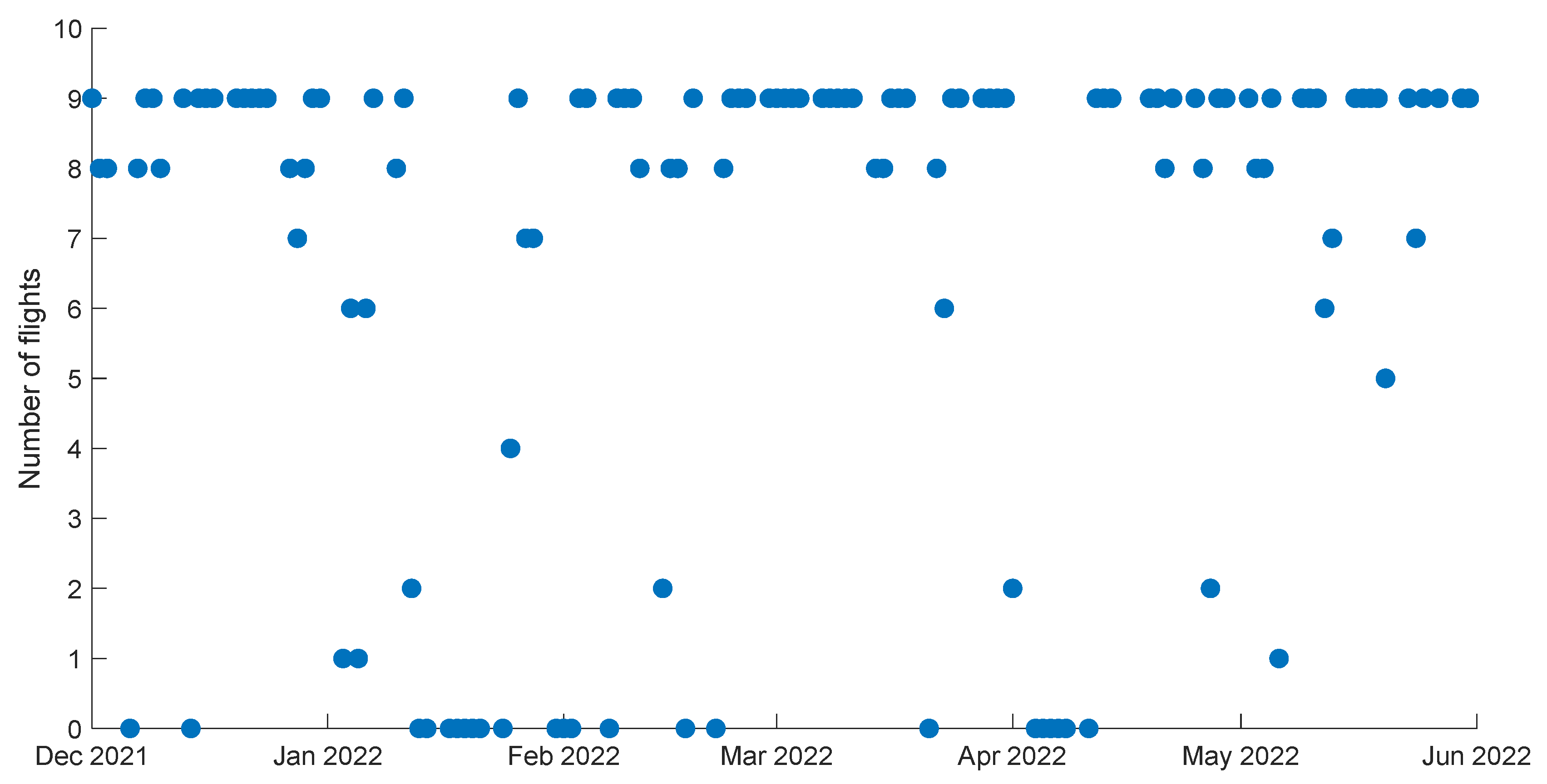
During the main campaign between December 2021 and May 2022, 864 flights were performed (
Table 1). With 128 working days during this period and eight flights planned per 24 h, a total of 1024 flights were scheduled to be performed, giving an availability of 75.7% (
Figure 2). On 87 nights, flights were performed according to schedule, with at least eight flights per night (68%). This availability was below the 95% availability expected for international operational profilers networks like E-PROFILE [
48].
Of the missing flights, 50.3% were not performed due to technical problems, 22.8% due to weather conditions, and 26.9% due to airspace restrictions. Around 10 flights encountered a major technical problem that required manual intervention to return the drone to its base. In January 2022, a motor failure led to a second emergency landing, which damaged the drone. In total, five different drones were used to continue measuring after technical difficulties.
During the same period, the availability was 95% for the Doppler LiDAR, 94.3% for the radar wind profiler, 99.3% for the microwave radiometer, and 70.2% for the Raman LiDAR.
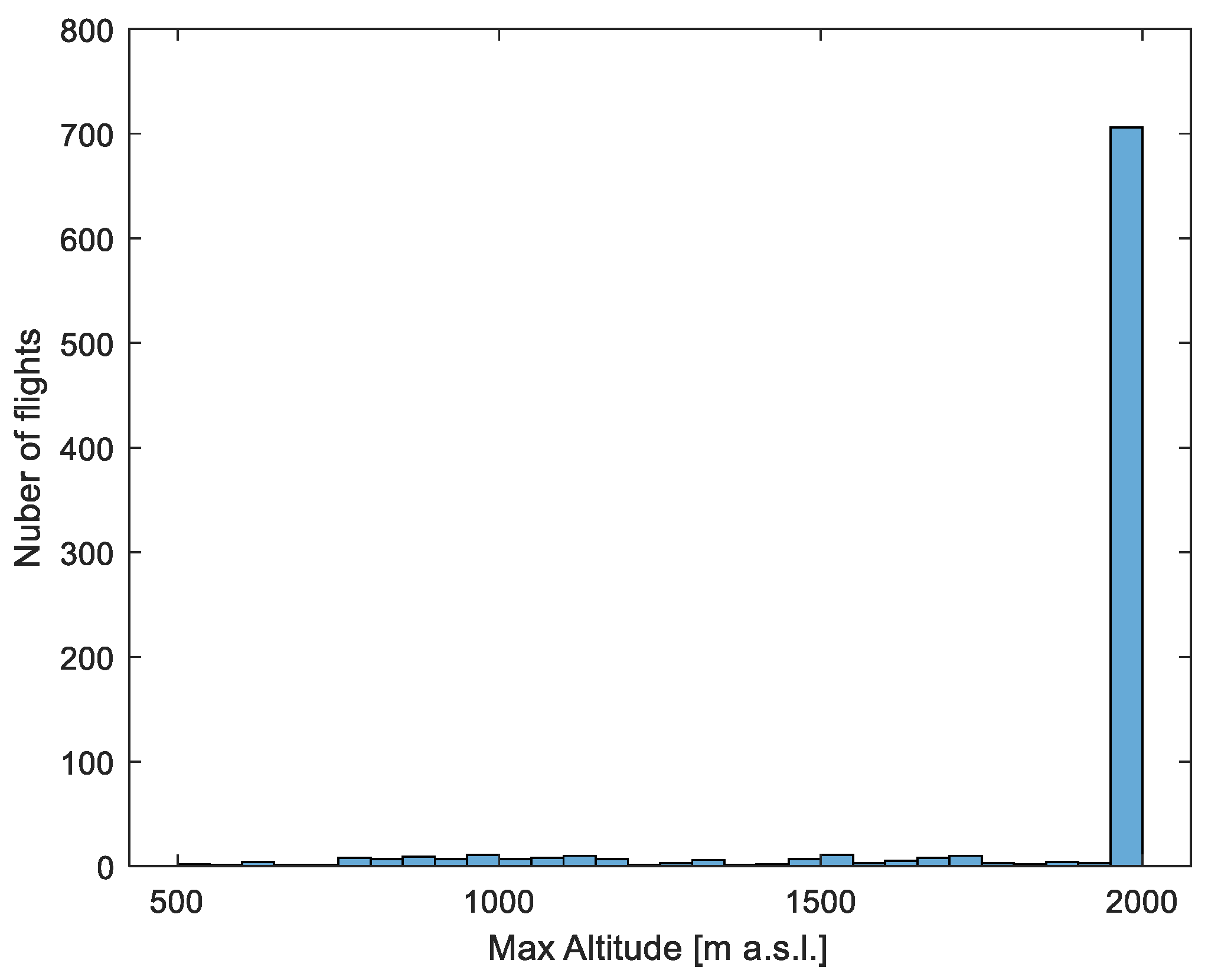
In total, 709 flights (82.1%) reached the nominal altitude of 2000 m above sea level (
Figure 3). The remote Meteodrone operator aborted the remaining 155 flights (17.9%), mostly due to delicate atmospheric conditions, such as high wind speeds. The maximum wind speed recorded by the wind LiDAR during the operations was 31.3 m.s
−1, suggesting that the drone flew above the theoretical limit of 25 m.s
−1. The minimum temperature recorded by the microwave radiometer between the ground and 2000 m was −11.2 °C.
In total, 91.3% of the flights were performed within 10 min of the nominal time. Data were transferred in real-time to the MeteoSwiss server, and 92.6% of the files were available on the MCH server within 10 min.
3.2. Case Study 1: 24 May 2022
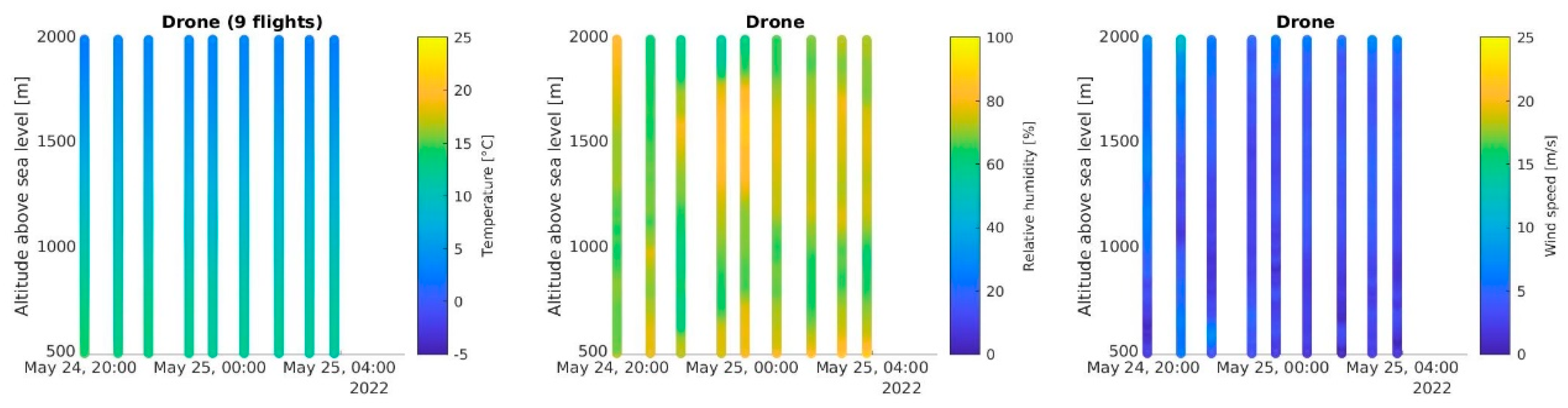
During the night from 24 to 25 May 2022, nine flights were performed. The overview of the measurements is shown in
Figure A1.
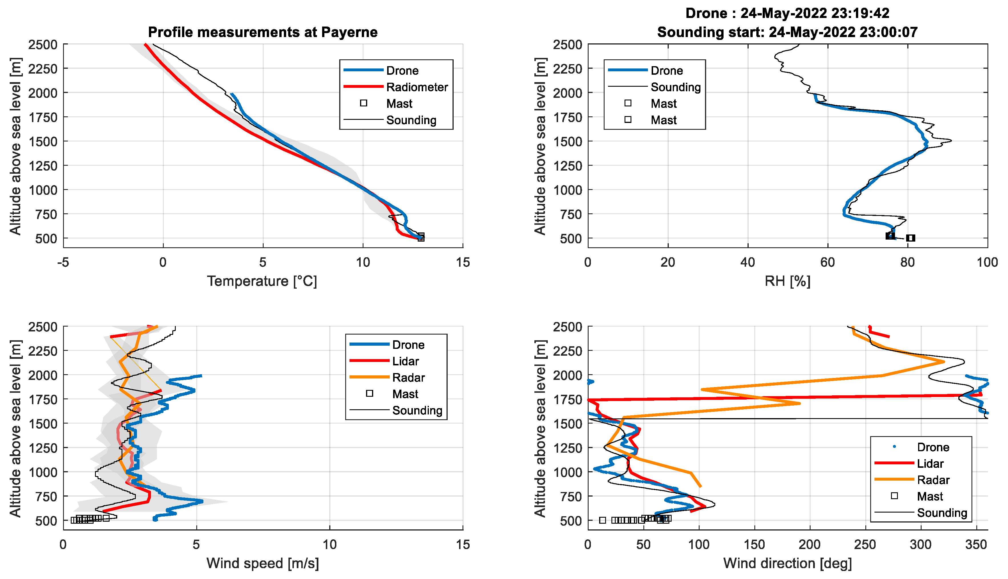
Figure 4 shows the profiles recorded by the radio sounding at 23:00 UTC and at 23:19 UTC by the drone. In blue, the Meteodrone measurements are presented, with the radio soundings in black and the remote sensing measurements in red.
Figure 4 shows temperatures of around 13 °C at the ground, decreasing to 4 °C at 2000 m, with a small temperature inversion at around 750 m a.s.l. All instruments show the temperature inversion, but the sounding reported a more detailed structure compared to the other instruments. A humid layer was measured around 1500 m with a maximum relative humidity of around 90%. That night, the Raman LiDAR RALMO was not operational; therefore, there is no humidity profile measured by a remote sensing instrument displayed in
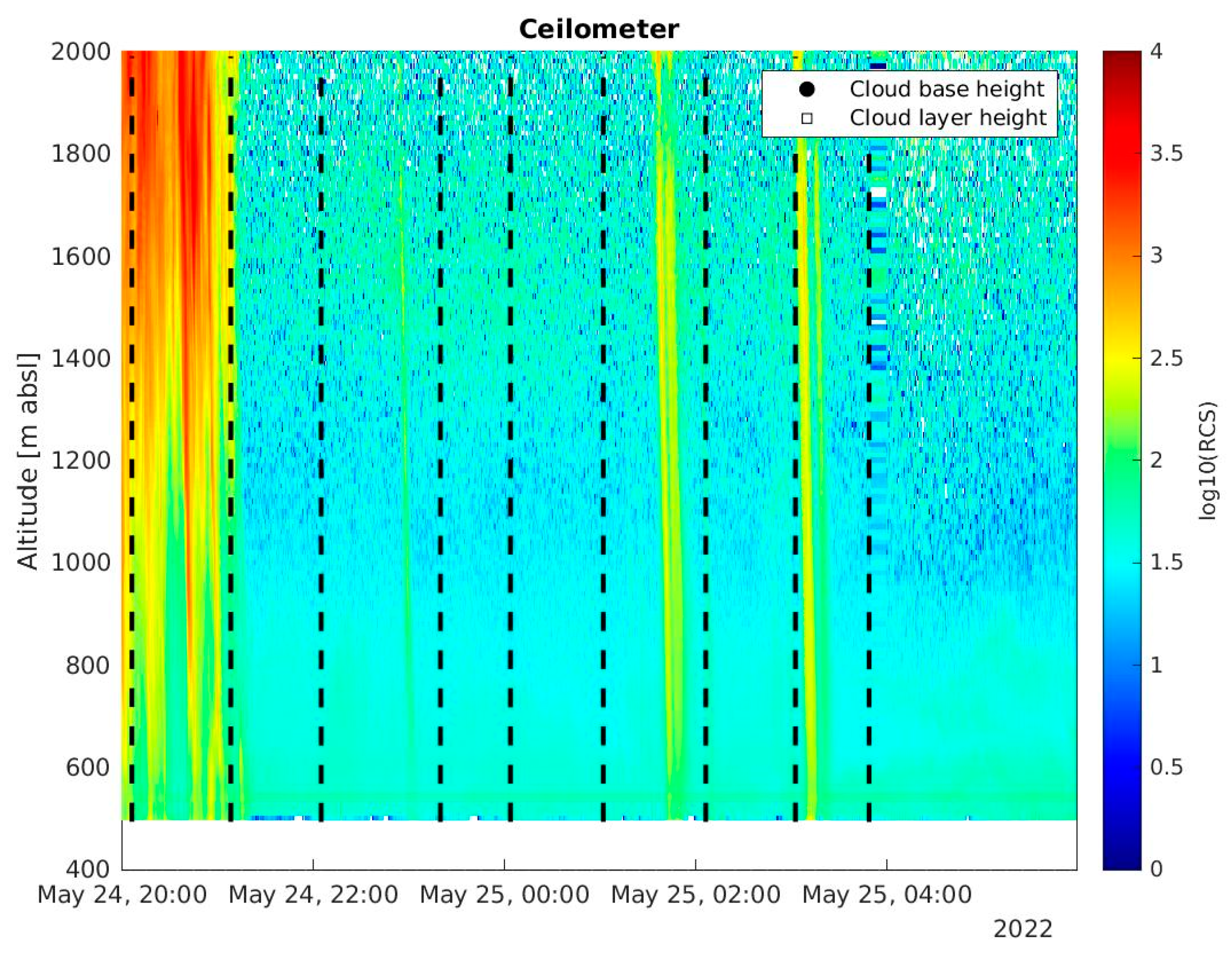
Figure 4. Light precipitation was recorded at the beginning of the night (
Figure A2). The wind speed was low, with values below 5 m.s
−1. All instruments provided comparable results, even though the drone overestimated the wind speed by 1.2 m.s
−1 (67%) on average for this profile. The wind direction was shifting from easterly winds at the ground to northerly winds at 1500 m a.s.l.
This case study highlights the good data quality a Meteodrone can achieve. It provides profiles of the temperature, humidity, and wind in the boundary layer with a higher temporal frequency compared to a radio sounding. It is also providing these measurements with one instrument instead of having different remote sensing instruments.
Nevertheless, as for all instruments, there were some drawbacks: Case study 2 illustrates challenges that were encountered with the Meteodrone.
3.3. Case Study 2: 15 December 2021
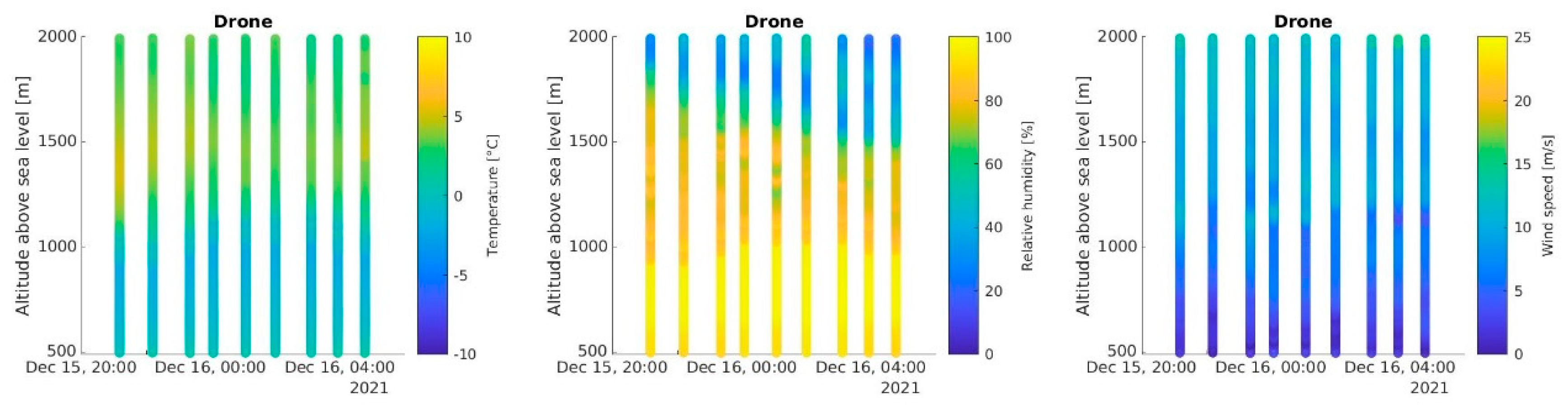
On the night between 15 and 16 December 2022, nine flights were performed. The overview of the measurements is shown in
Figure A3.
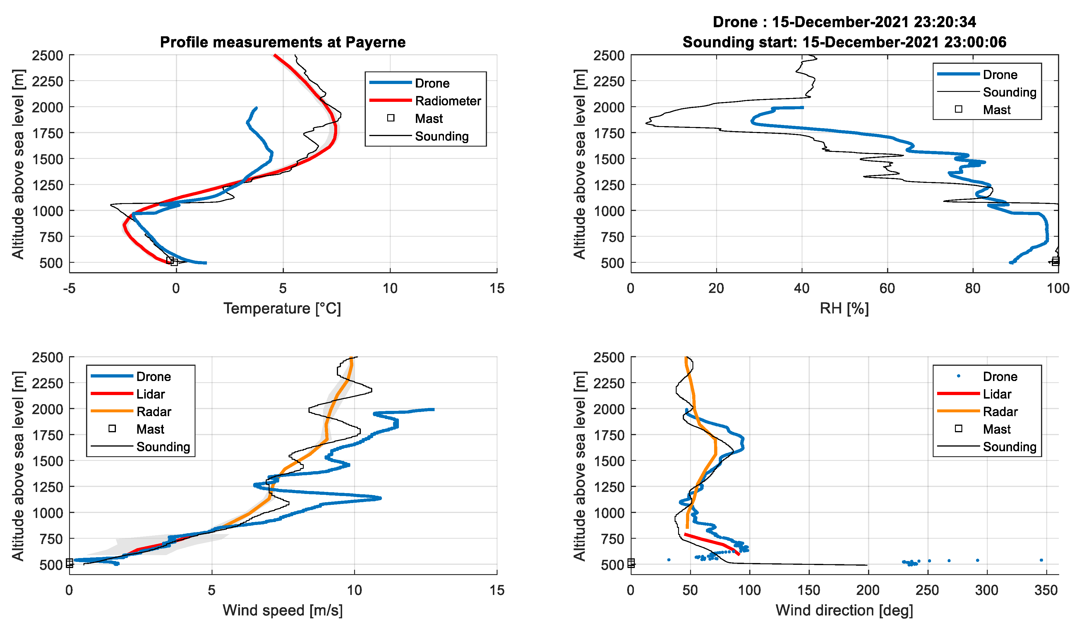
Figure 5 shows the profiles recorded by the radio sounding at 23.00 UTC and at 23:20 UTC by the drone. In blue, the Meteodrone measurements are presented, with the radio soundings in black and the remote sensing measurements in red.
Figure 5 shows the temperature was around 0 °C at the ground, decreasing to −3 °C at 1000 m, with an important temperature inversion above and a maximum temperature of 7.7 °C at 1916 m. All instruments showed the temperature inversion, but the sounding again reported a more detailed structure. The minimum and the maximum of the remote sensing measurements between 23:00 UTC and 23:30 UTC are represented by the grey areas, showing that the conditions were steady over time during the case study. Thus, the differences between the radio-sounding and the Meteodrone cannot be attributed to atmospheric variability.
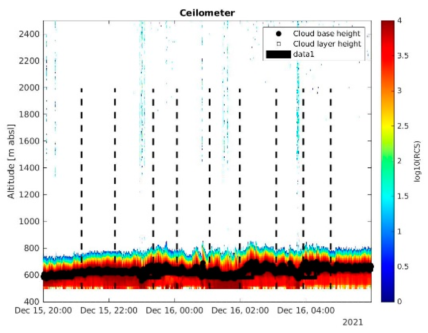
A thick stratus was present this night, with a cloud base height reported by the ceilometer at 530 m (
Figure A4). It was confirmed by the relative humidity of 100% from 660 m to 1060 m in the radiosonde relative humidity measurements. That night, the Raman LiDAR RALMO was not measured because of the low clouds; therefore, there is no humidity profile measured by a remote sensing instrument in
Figure 5.
The Meteodrone did not measure a relative humidity above 97.4%, even though the sensor seemed saturated between 700 m and 900 m. Similar underestimations of high relative humidity were observed on several occasions at the beginning of the campaign: the Meteodrone never measured 100% in December, even in clouds.
The dry layer around 1800 m was detected by the Meteodrone but with a relative humidity of 25% instead of 4.6%. This was likely due to the overestimation of the temperature at this altitude or contamination of the sensor. According to Meteomatics, the positioning of the sensor was not ideal and might have led to the contamination of the measurements. The location of the sensor was changed later in January. In terms of the specific humidity, the Meteodrone reported a minimum of 1.67 g.m−3 instead of the 0.3 g.m−3 measured by the radio sounding. Due to this major difference, this case was excluded from the humidity analysis in this document.
The wind speed at the ground was low, progressively increasing to 10 m.s−1 at 2500 m. All instruments provided comparable results, even though the drone overestimated the wind speed by 1.18 m.s−1 (20%) on average; the wind LiDAR measured in the lower part of the stratus, and the wind radar measured above. The wind direction was relatively constant with northeasterly winds.
3.4. Temperature Evaluation
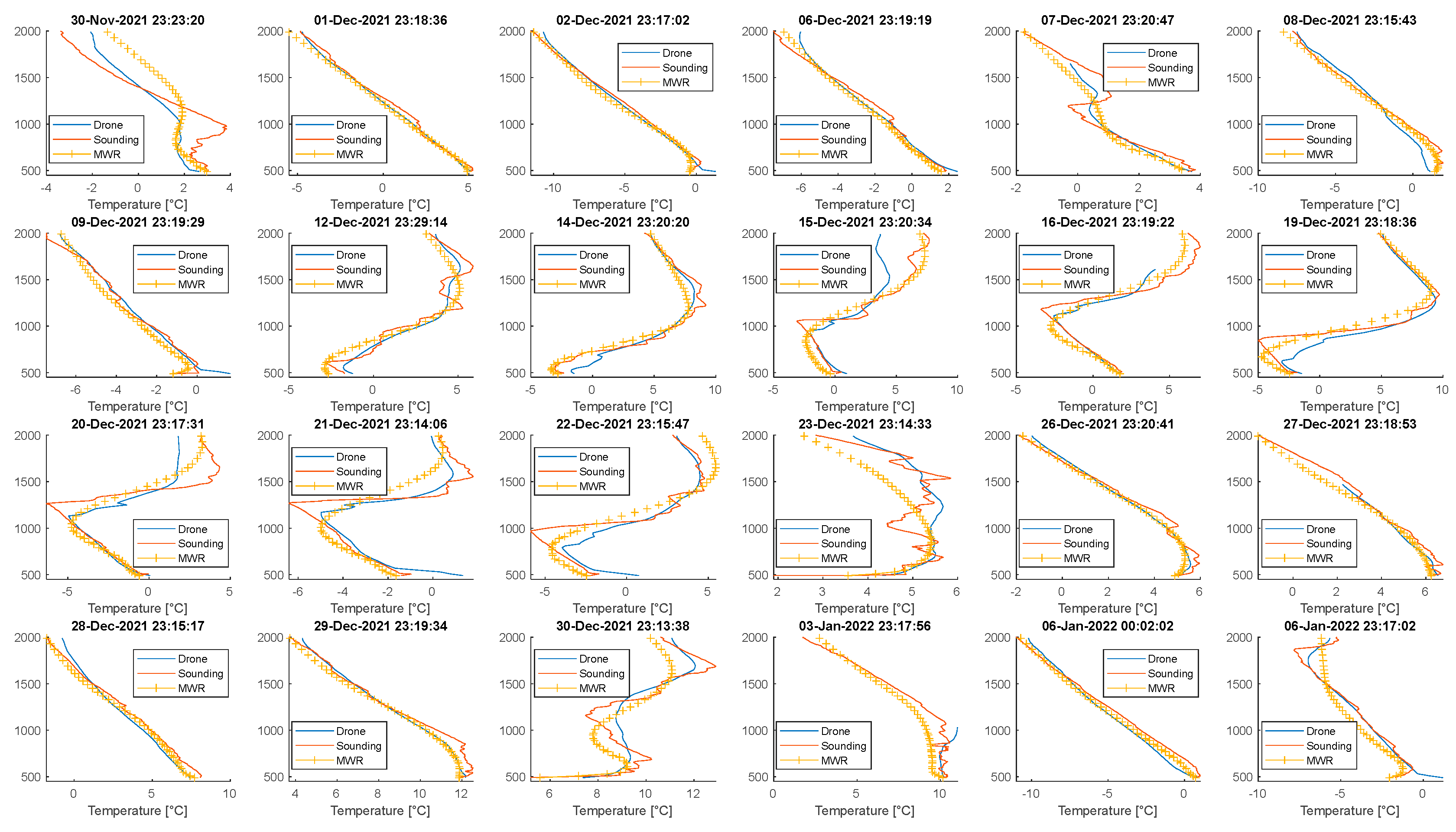
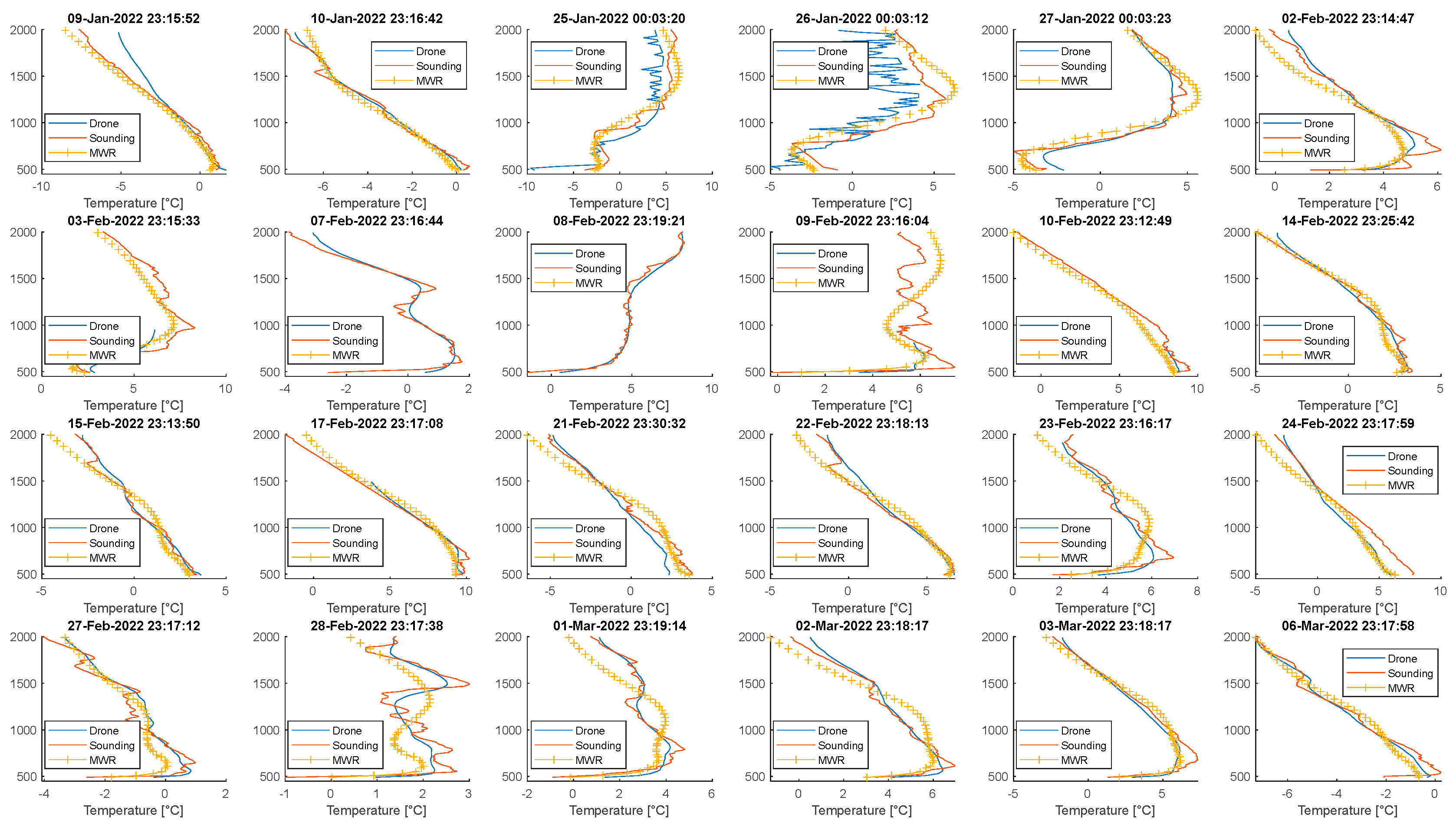
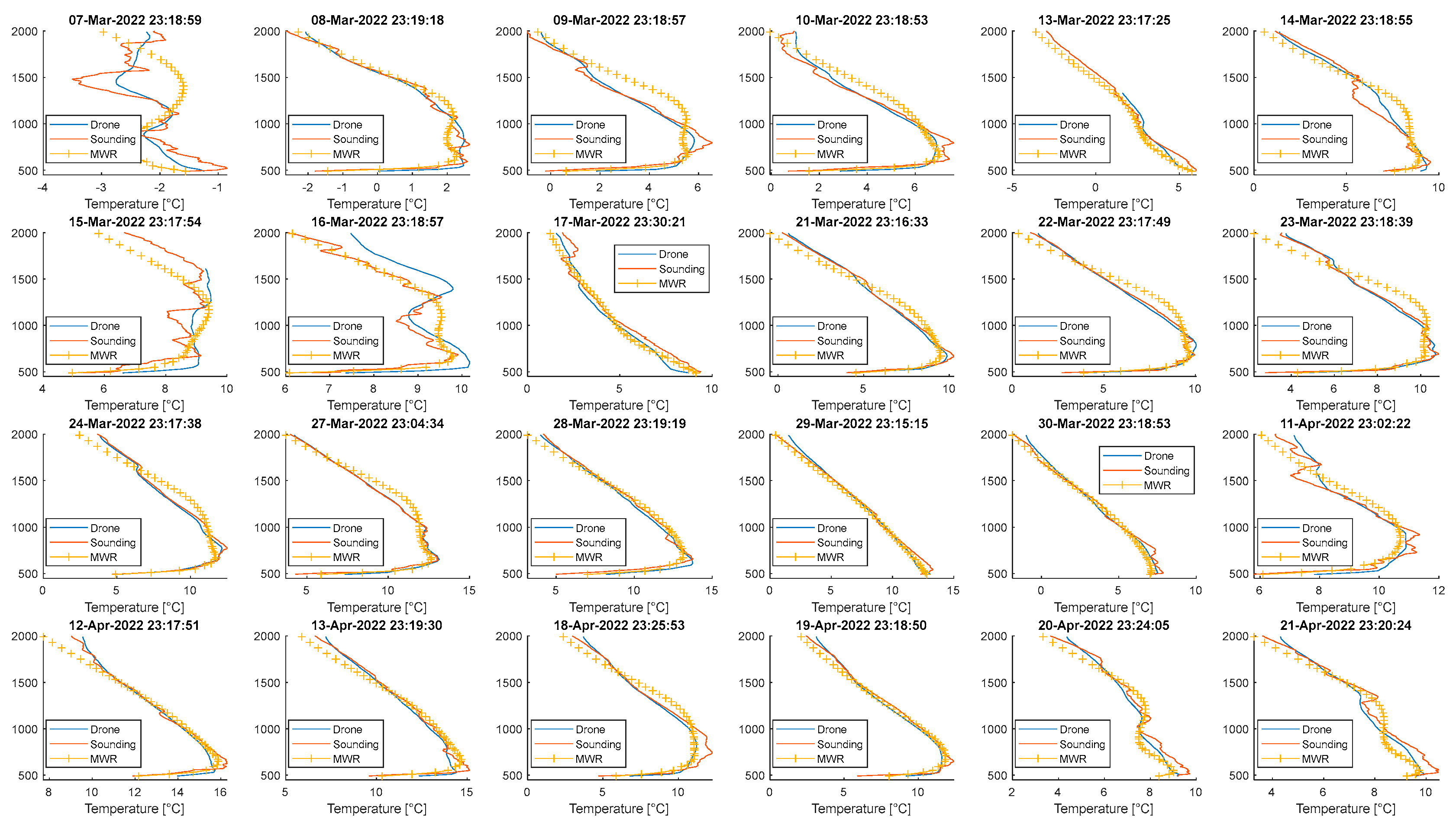
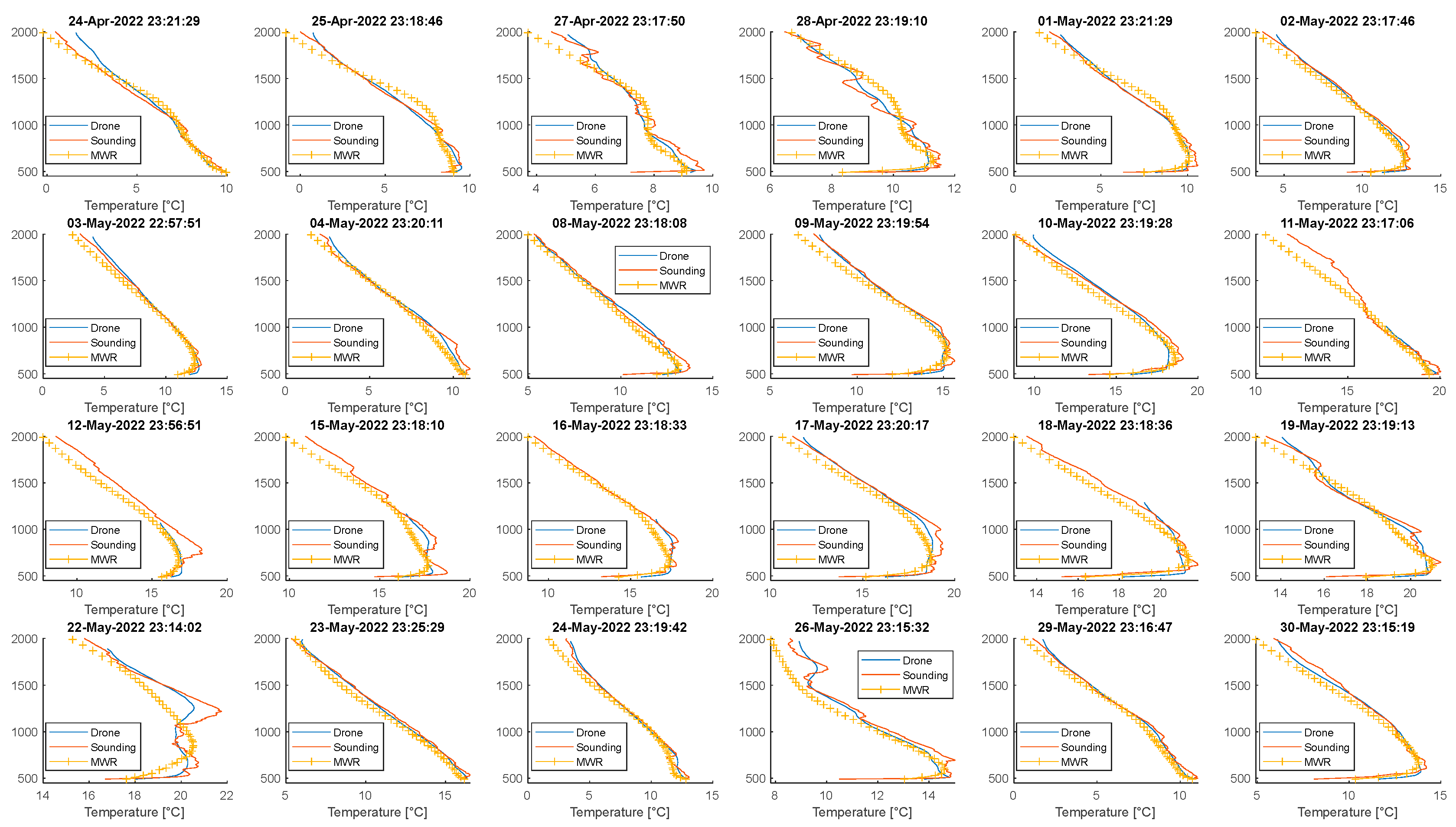
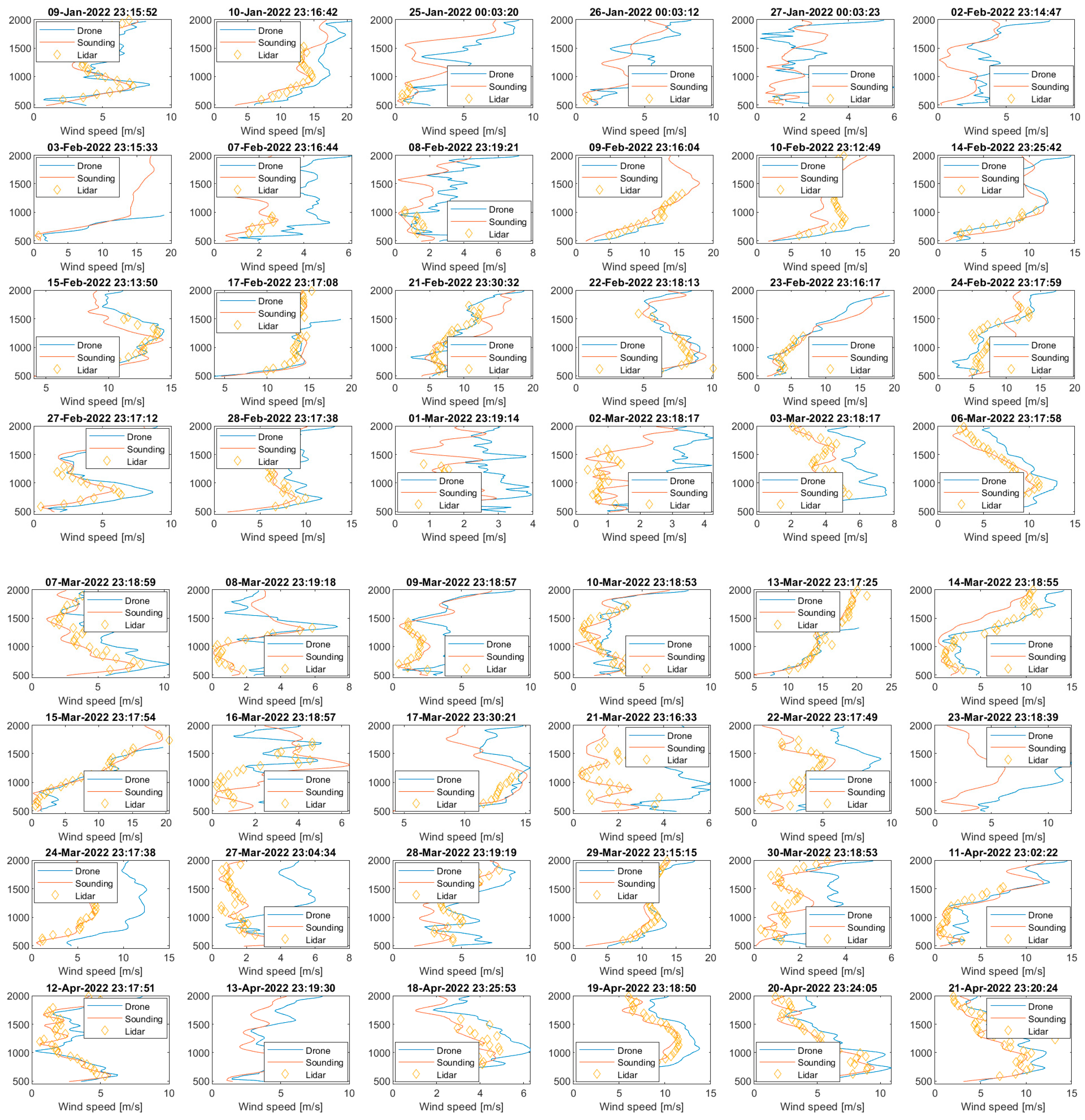
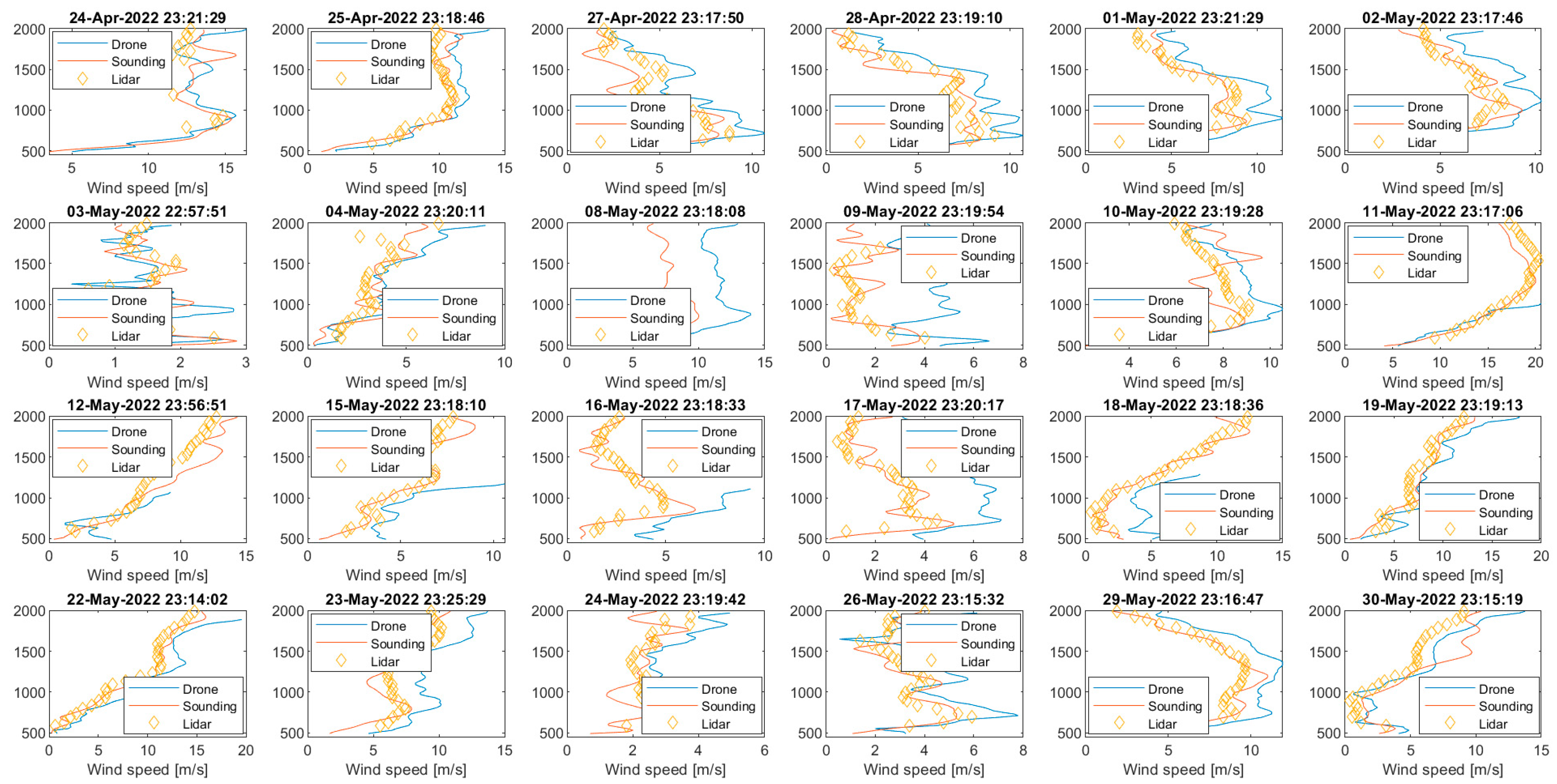
In order to provide a quantitative evaluation, the measurements from Meteodrones and remote sensing instruments were compared to the radiosoundings. In total, 97 flights were performed around 23:15 UTC, close to the radiosonde launch. These profiles are visible in
Figure A5 and
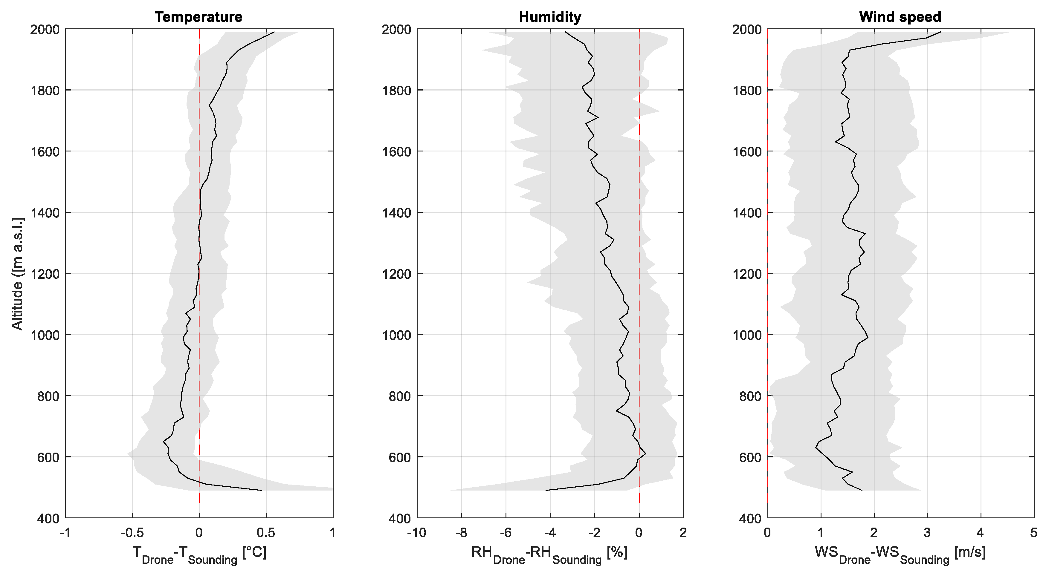
Figure A6. The difference between the profiles was calculated for the temperature, relative humidity, and wind speed, and the vertical profile of these differences is visible in
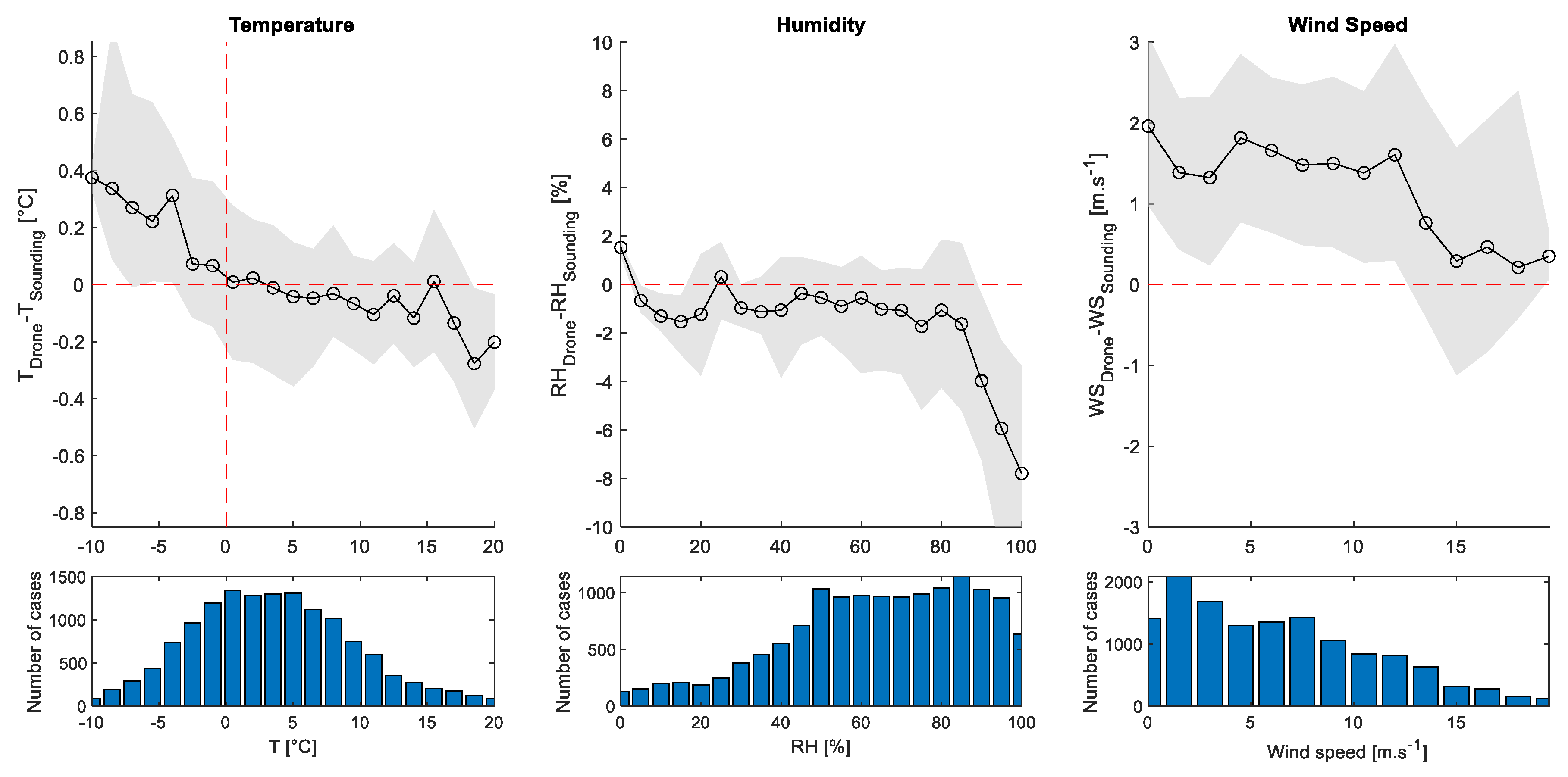
Figure 6. The differences in the temperature, relative humidity, and wind speed according to the value measured by the radiosonde are shown in
Figure 7.
In
Figure 6 and
Figure 7, the agreement between the Meteodrone and the radiosonde is visible, with median differences lower than 0.5 °C. Even though the average bias was close to zero (−0.01 ± 0.66 °C), some biases for temperature were visible at the bottom and the top of the profile. It is likely that the overestimation close to 0.5 °C at low altitude was due to the effect of the Meteobase, which keeps the drone at a controlled temperature before launch, affecting the lower part of the measurements. Bärfuss et al. [
21] also described a significant difference close to the ground and attributed this difference to the lack of ventilation before the launch. Koch et al. [
15] similarly reported a warm bias of 0.4 °C when comparing a Meteodrone-SSE with respect to the balloon data over 37 flights over 5 days. Inoue et al. [
14] reported a warm bias in the range of 0.3–1.0 °C among almost all profiles and all layers with a mean difference of 0.68 °C (±0.39 °C) between a radiosonde RS41-SGP and a Meteodrone MM670 [
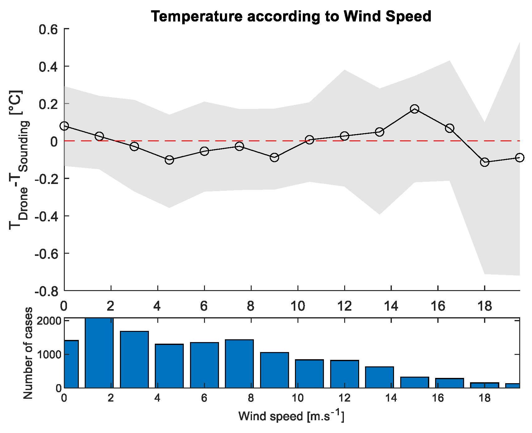
14]. That comparison was limited to seven daytime soundings up to 750 m above ground level. They reported the impact of the radiation of the temperature sensor. This effect could not be visible at Payerne, as the flights were performed only during night-time. They also attributed the warm bias at the bottom of the profile to the time lag issue and the bias at the upper part of the profile to extra heat exhaust from the rotors and the UAS body under the conditions of high horizontal wind speed. At Payerne, no correlation between the observed bias and the wind speed was visible (
Figure A9), suggesting that higher horizontal winds had a limited impact on the quality of wind measurements.
At Payerne, the temperature bias increased from −0.27 °C at 650 m to 0.56 °C at 1990 m (
Figure 6). This warm bias was visible only for negative temperatures (
Figure 7), suggesting that the impact of the drone was greater at low temperatures. In particular, the impact of the heating of the propeller cannot be excluded, as this heating is turned on only in freezing conditions. Meteomatics performed a test to study the impact of the propellers’ heating on the temperature profile (personal communication, 2023). This test did not show a visible impact compared to the numerical weather forecasts, suggesting that the heating impact was limited.
To fully investigate the origin of the reported biases, more detailed data would be needed, for example, the variability between the three temperature sensors, the difference between the up and down measurements, the inclination and the heading of the drone, or the intensity of the heating on the propellers. These data were not provided by Meteomatics for this campaign.
3.5. Humidity Evaluation
To evaluate the performance of the humidity measurements, eight suspicious profiles were excluded:
Three cases with a dry layer above fog that was not correctly measured (15, 16, and 20 December 2021). As discussed in case study 2, contamination of the humidity sensor was reported by Meteomatics and might be the origin of these differences with an RMS for specific humidity differences reaching values up to 285% on 20 December 2021;
Four cases where the humidity of the sensor was not recorded correctly (24, 25, and 26 January 2022 and 16 March 2022);
One case with a very dry layer (RH < 1.6% measured by the radiosonde and RH < 6.95% measured by the Meteodrone on 28 February 2022) led to a significant difference in terms of the specific humidity (72%). This result was not representative of the performance of the Meteodrone that day, as the relative humidity measured by the Meteodrone was close to the one measured by the RS41 (see
Figure A6).
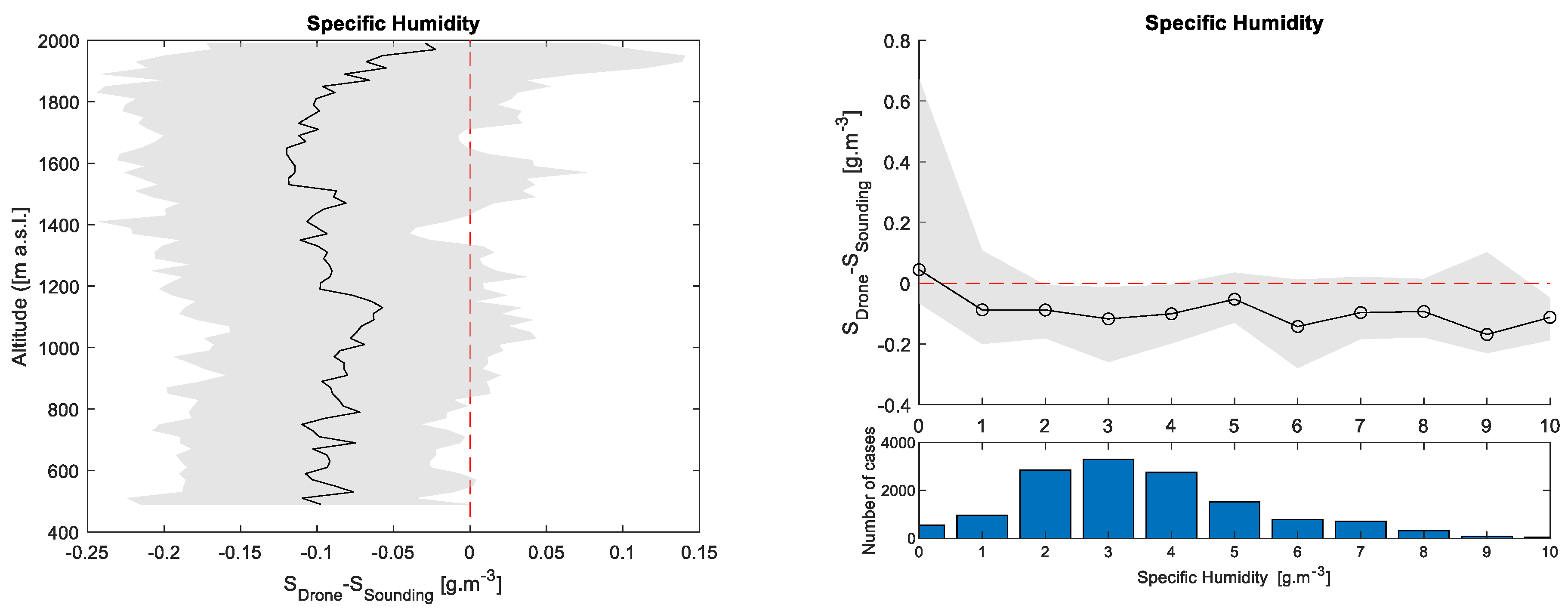
On average, the relative humidity was underestimated by the Meteodrone by −1.6% (±7.3%). As with the temperature, biases were visible at the bottom and the top of the profile. Close to the ground, the relative humidity was underestimated by −4%; it reached 0% at 600 m and decreased with the altitude reaching −3.3% at 1990 m. This effect was not visible on the specific humidity profile (
Figure A10), with a relatively constant difference of −0.10 (±0.23 g.m
−3).
Figure 7 demonstrates that the RH difference was more significant when the relative humidity was closer to saturation, with an underestimation of up to −7.8%. Therefore, the relative humidity biases seemed linked to two effects: first, the temperature overestimation, and second, the underestimation of the relative humidity in clouds, as mentioned in case study 2. These results were of the same order of magnitude as the results of the LUCA drone that reported a mean bias of 2.73% (±8.67%) compared to radiosondes [
21] or as in the evaluation of 38 UAVs showing that the relative humidity was in general lower (−3.15% ± 12.12%) than the reference values [
22]. Moisture is the most difficult atmospheric parameter to measure in flight [
21]. It requires significant post-processing to obtain accurate results [
50,
51]. Unlike RS41 radiosondes, the Meteodrone sensors were not calibrated before each flight, and drifts, or contaminations might be difficult to identify if there is no co-located reference. Again, having access to additional data like the variability of the two humidity sensors would be useful for a finer analysis, but it was not provided by Meteomatics for this campaign.
3.6. Wind Evaluation
Figure 6 shows that the wind speed was overestimated by the Meteodrone. The bias was nearly constant around 1.5 m.s
−1 up to 1900 m, but the value increased at the top of the profiles with a median overestimation of 3.25 m.s
−1. The overestimation of the wind speed at the top of the profile is known by Meteomatics and is attributed to the lower stability of the drone when it is changing direction (personal communication, 2023). This overestimation was often visible (
Figure A7) even when the drone was not at 2000 m, like on 3 February, 17 February, or 15 May 2022.
Figure 7 suggests that the overestimation was otherwise mostly constant (+1.57 m.s
−1) for wind speeds up to 12 m.s
−1. At higher wind speeds, the agreement improved with a mean difference of +0.42 m.s
−1. For the wind LiDAR, the mean wind difference was −0.14 m.s
−1, suggesting a better performance of the LiDAR. Koch et al. [
15] reported an average bias for Meteodrone-SSE of +0.2 m s
−1. This suggests that the performance of the wind speed measurements with a Meteodrone-670 could be improved, as the technique to retrieve the wind speed was similar between the two instruments. Better results were also obtained with the LUCA drone with a mean difference of −0.39 m.s
−1 (±1.15 m.s
−1) [
21], suggesting that the pitot tube can be an accurate tool for retrieving wind profiles. For the wind direction, the mean difference was 10.6° with a standard deviation of 45.3°. This can be compared with a mean wind direction difference of −1.8° for the wind LiDAR and a standard deviation of 30°. Koch et al. [
15] reported a mean error of 6° and Bärfuss et al. [
21] a mean difference of 0.62° ± 5.05° suggesting that good performances can be achieved with drones. Meteomatics mentioned that the algorithm was not updated after a drone modification, and the results should be better in an updated version of the algorithm (personal communication, 2022). As the wind speed is based on the propellers’ speed adjustments, a minor modification to the drone can lead to significant differences in the wind estimation. Meteomatics is working on a bias correction to improve wind estimation.
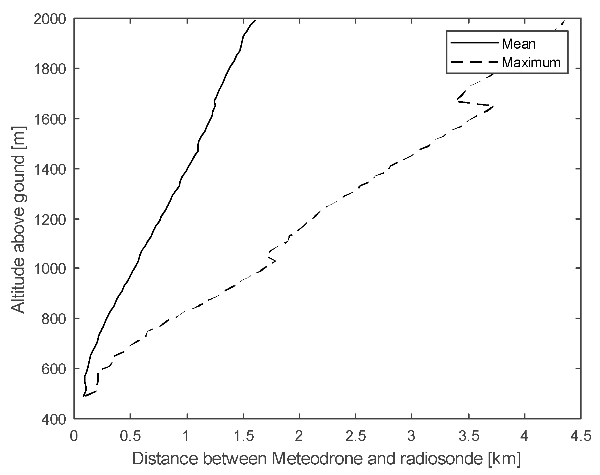
3.7. Temporal and Spatial Variability
As explained in
Section 3, there was a 15 min delay between the radiosonde and the other measurements. The impact of this delay was assumed to be negligible as the analysis was performed over 97 profiles under different atmospheric conditions. Moreover, the bias shown by the Meteodrones was not visible on the remote sensing instruments that were evaluated at the same time as the Meteodrones. The variability of the atmospheric conditions was shown in case study 2, suggesting that this variability was not the main factor of the differences between the sounding and the Meteodrone. Similarly, the impact of the distance between the radiosonde and the Meteodrone was assumed to be small, as the average distance was 0.77 km with a maximum of 4.3 km (
Figure A8). This evaluation of the Meteodrone was more restrictive in terms of the spatial and temporal variabilities than the evaluation of the LUCA drones [
21] or the AMDAR data [
52], which both used a threshold of 50 km and 30 min difference.
Figure 6 does not exhibit a clear trend with altitude, suggesting again that the spatial variability was not the main factor in the differences reported above.
3.8. WMO Requirements
In order to provide a quantitative evaluation of the potential of the Meteodrone to be assimilated in high-resolution NWP, the WMO requirements were used, as described in
Section 2. The WMO requirements for the temperature, humidity, and wind are presented in
Table 2, together with the RMS of the differences between the Meteodrones and radiosounding as well as the RMS of the differences between the remote sensing instruments and the radiosounding.
As shown in
Table 2, the Meteodrones and HATPRO-G5 radiometers meet the “breakthrough” target for temperature with an RMS smaller than 1 K. When comparing the Meteodrone to the radiometer, similar results were obtained with an RMS of 0.79 K. Both technologies are, therefore, suitable for assimilation into NWP models.
For the humidity evaluation, after filtering the inaccurate profiles, the RMS for specific humidity was 8.3%, which met the threshold requirement of 10%. The Raman LiDAR presented comparable results with a slightly higher uncertainty estimated at 9.2%. Using a similar technique, Gaffard et al. [
49] evaluated a Dial LiDAR and reported an uncertainty between 5% and 10%, suggesting similar performances. When comparing the Meteodrone to the Raman LiDAR, similar results were obtained with an RMS of 9.02%. In terms of the relative humidity, the uncertainty was 5.81%RH for the Meteodrone and 5.56%RH for the RALMO.
For the wind, the root mean square vector difference (RMSVD) calculated for the Meteodrone was 3.1 m.s
−1, suggesting that the Meteodrone’s data were suitable for assimilation into NWP models but could be improved. The value was significantly better for the wind LiDAR with an RMSVD of 1.8 m.s
−1, meeting the “breakthrough” requirement. The RMSVD between the drone and the wind LiDAR was 2.71 m.s.
−1, suggesting that the difference between the drone sounding does not come from the temporal or spatial variabilities. Bärfuss et al. reported an RMSVD of 0.97 m.s
−1 [
21], reaching the “goal” and suggesting that this requirement can be achieved with a UAS.
3.9. Time Evolution
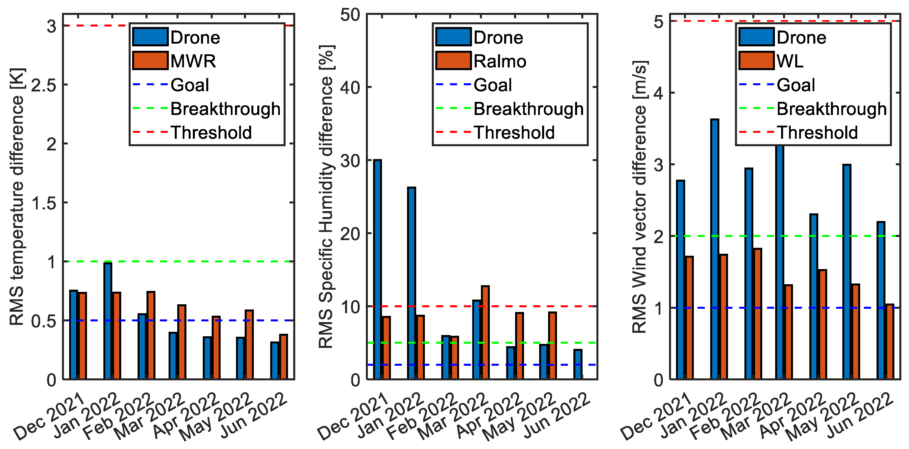
Figure 8 represents the monthly average of the differences between the radiosoundings and Meteodrones or remote sensing instruments, respectively. The RMS of the temperature difference evolved from 0.75 K in December to 0.31 K in May. This improvement can be partly explained by the meteorological conditions that were more favourable to drone measurements without the need to heat the propeller and a smaller temperature difference between the air and the drone. For the radiometer, the evolution of the RMS of the temperature difference was smaller: from 0.73 K to 0.58 K. This suggests that the improvement seen in the RMS of the Meteodrone was partly due to technical improvements made during the campaign. For the humidity, the evolution was even greater, with an RMS of the specific humidity difference of 30.0% in December and 4.7% in May. The significant differences observed in December and January could be explained by chemical contamination on the humidity sensor leading to a bias like that observed by Wang et al. [
53] on radiosondes. It is likely that the replacement of the sensors on 31 January 2022 clearly improved the performance of the Meteodrone. In comparison, the performance of the Raman LiDAR was stable, with an RMS of 8.55% in December and 9.1% in May.
For the wind, the evolutions of the RMS of the wind vector difference from 2.7 m.s−1 in December to 3.0 m.s−1 in May for the Meteodrone and 1.71 m.s−1 in January to 1.32 m.s−1 in May for the Doppler LiDAR do not demonstrate a clear trend for the two instruments.
4. Conclusions
For the first time, an extensive automatic drone campaign was conducted over a 6-month period, and the results were compared to co-located radiosoundings. A total of 864 automatic flights were performed during the campaign, resulting in an availability rate of 75.7%, below the 95% availability expected by international profiler networks like E-PROFILE. Among the flights, 82.1% reached the nominal altitude of 1500 m above ground. To ensure optimal availability and quality, five different Meteodrones were used by Meteomatics throughout the campaign, and several adjustments were made during the campaign, including sensor replacements after 31 January 2022.
Two case studies were selected, one demonstrating the performance of the Meteodrone and another one illustrating the challenges encountered during the campaign, like measuring within and above clouds or wind speed overestimation.
The quality was analyzed for 97 flights performed at the same time as the Vaisala RS41 radiosoundings. The results were contextualised using the same methodology applied to the remote sensing measurements. Based on these findings, the Meteodrone meets WMO’s “breakthrough” requirements for high-resolution NWP in terms of temperature. The Meteodrone also meets the minimum WMO requirements for wind and humidity after excluding eight cases where the humidity sensor did not perform optimally. The classifications for temperature and humidity derived from this campaign measurements are the same for remote sensing instruments. The wind LiDAR, however, performed better than the Meteodrone wind measurement during this experiment, reaching the “breakthrough” requirement.
Therefore, Meteodrones, like remote sensing instruments, can be assimilated into NWP models and are interesting tools to measure temperature, humidity, and wind profiles with a high temporal and vertical resolution under a wide range of meteorological conditions.
The Meteodrone is now operated at Payerne by Meteomatics in the framework of the DETAF 2.0 project. On 1 August 2023, 1393 flights in total were performed by Meteomatics at Payerne. In a project not financed by MeteoSwiss, Meteomatics plans to install several stations in Switzerland in 2024. One of the aims is to assimilate these data in a numerical weather prediction model to provide better forecasts.
The proof of concept presented in this study opens the door to operational measurements with drones to provide accurate meteorological observations in the boundary layer. It is the first step towards the worldwide demonstration campaign that will be organized by the WMO in 2024.
Author Contributions
Formal analysis, M.H.; writing—original draft preparation, M.H.; writing—review and editing, M.H., G.M., G.R., T.W. and A.H.; project administration, T.W. and A.H. All authors have read and agreed to the published version of the manuscript.
Funding
This research received no external funding.
Institutional Review Board Statement
Not applicable.
Informed Consent Statement
Not applicable.
Data Availability Statement
Data are available upon request.
Acknowledgments
The authors kindly acknowledge Meteomatics for performing the experiment and providing the Meteodrone data. We acknowledge MeteoSwiss staff for performing radio-sounding and remote sensing measurements, in particular Philipp Bättig, Daniel Bugnon, and Ludovic Renaud. This article is based on work from COST Action CA18235 PROBE, supported by COST (European Cooperation in Science and Technology)
www.cost.eu.
Conflicts of Interest
The authors declare no conflict of interest.
Appendix A
Figure A1.
Overview of the drone measurements during the night from 24 May 2022 to 25 May 2022. Left: temperature, middle: relative humidity, and right: wind speed.
Figure A1.
Overview of the drone measurements during the night from 24 May 2022 to 25 May 2022. Left: temperature, middle: relative humidity, and right: wind speed.
Figure A2.
Ceilometer measurements during the night from 24 May 2022 to 25 May 2022. Dashed lines represent the time when the Meteodrone was flying.
Figure A2.
Ceilometer measurements during the night from 24 May 2022 to 25 May 2022. Dashed lines represent the time when the Meteodrone was flying.
Figure A3.
Overview of the drone measurements during the night from 15 December 2021 to 16 December 2021. Left: temperature, middle: relative humidity, and right: wind speed.
Figure A3.
Overview of the drone measurements during the night from 15 December 2021 to 16 December 2021. Left: temperature, middle: relative humidity, and right: wind speed.
Figure A4.
Ceilometer measurements during the night from 15 December 2021 to 16 December 2021. Dashed lines represent the time when the Meteodrone was flying.
Figure A4.
Ceilometer measurements during the night from 15 December 2021 to 16 December 2021. Dashed lines represent the time when the Meteodrone was flying.
Figure A5.
Temperature profiles measured above Payerne. Blue: Meteodrone, red: radiosounding, and orange: microwave radiometer.
Figure A5.
Temperature profiles measured above Payerne. Blue: Meteodrone, red: radiosounding, and orange: microwave radiometer.
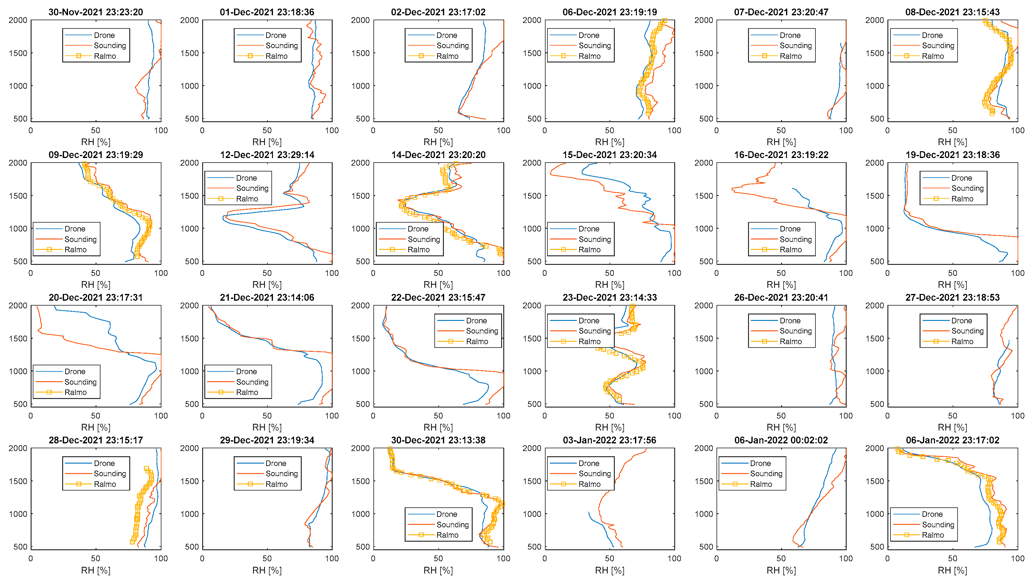
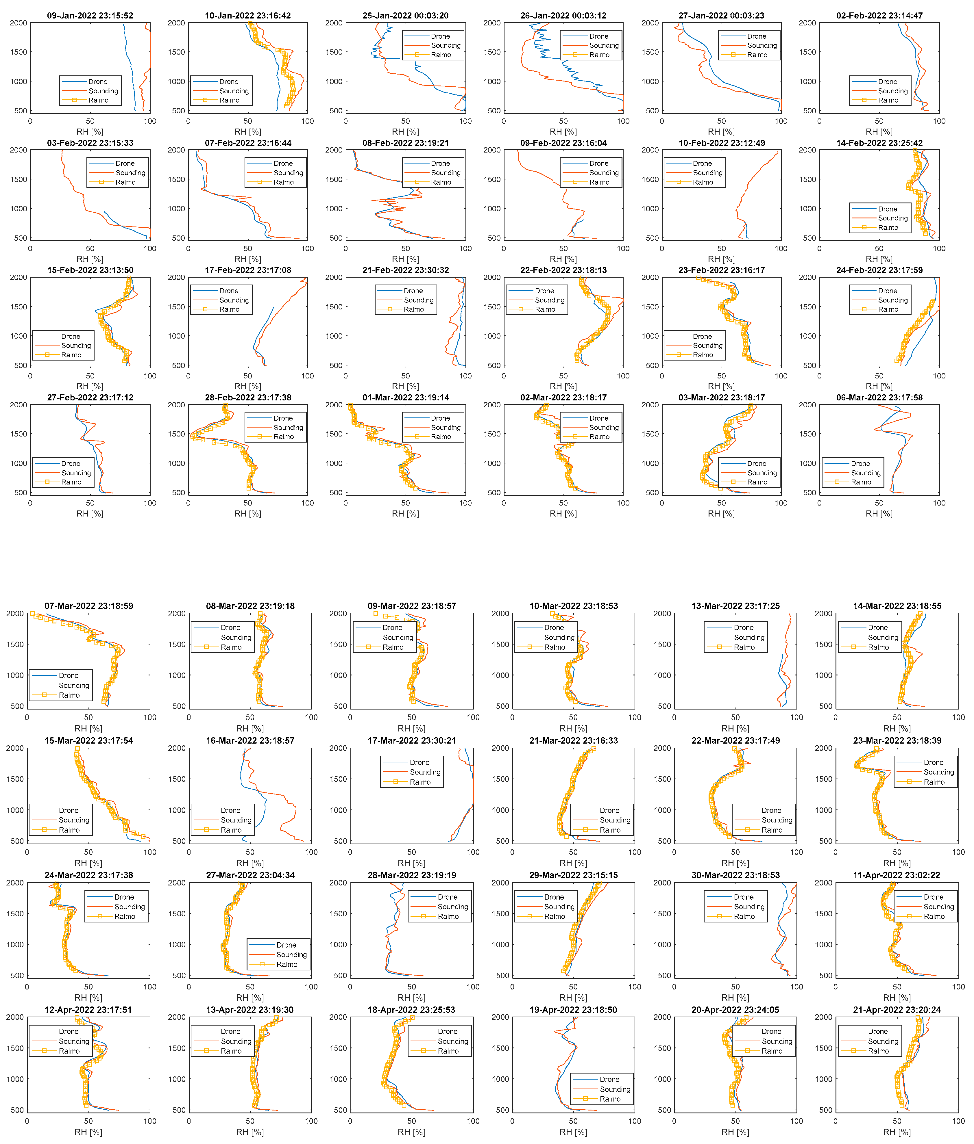
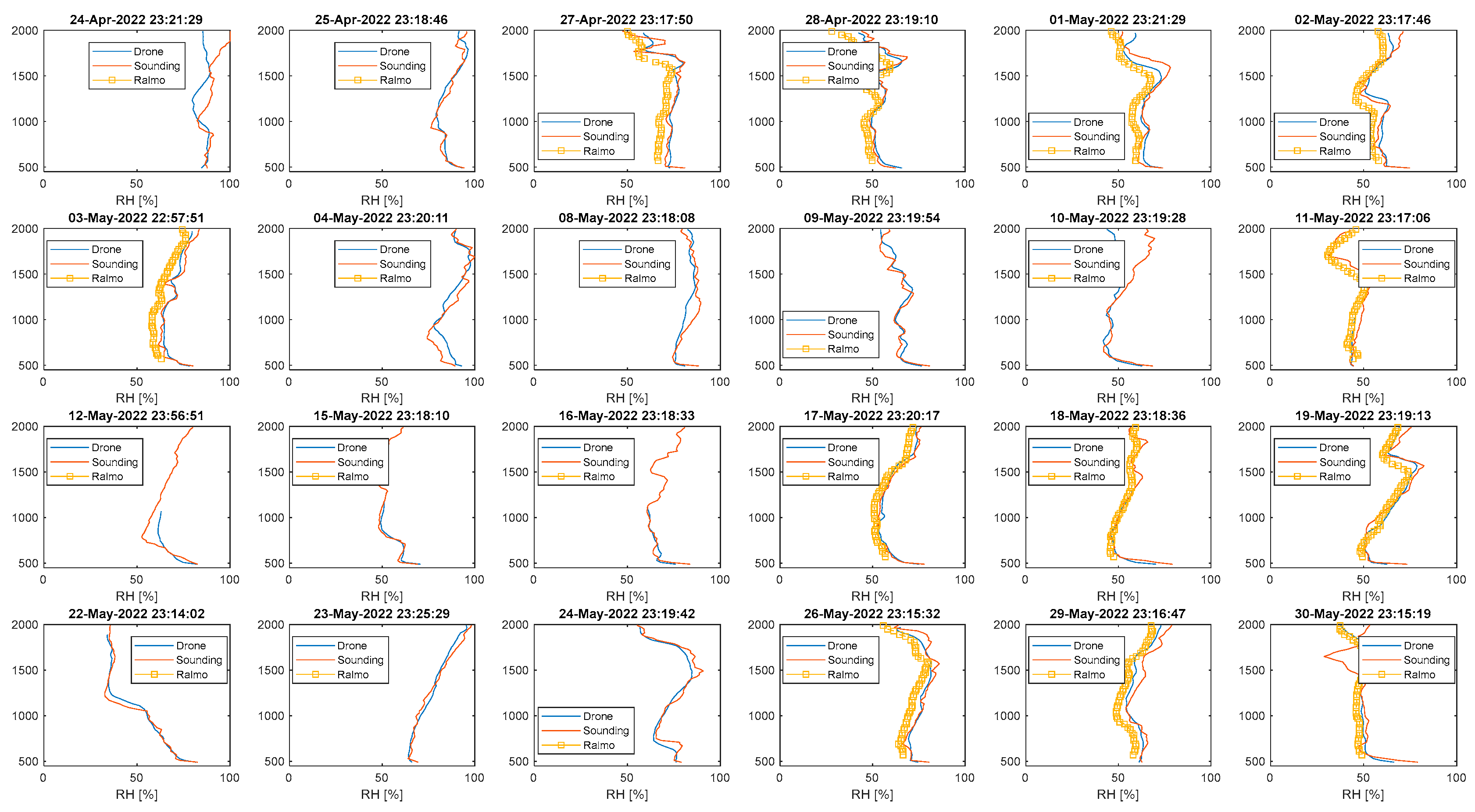
Figure A6.
Relative humidity profiles measured above Payerne. Blue: Meteodrone, red: radiosounding, and orange: Raman LiDAR RALMO.
Figure A6.
Relative humidity profiles measured above Payerne. Blue: Meteodrone, red: radiosounding, and orange: Raman LiDAR RALMO.
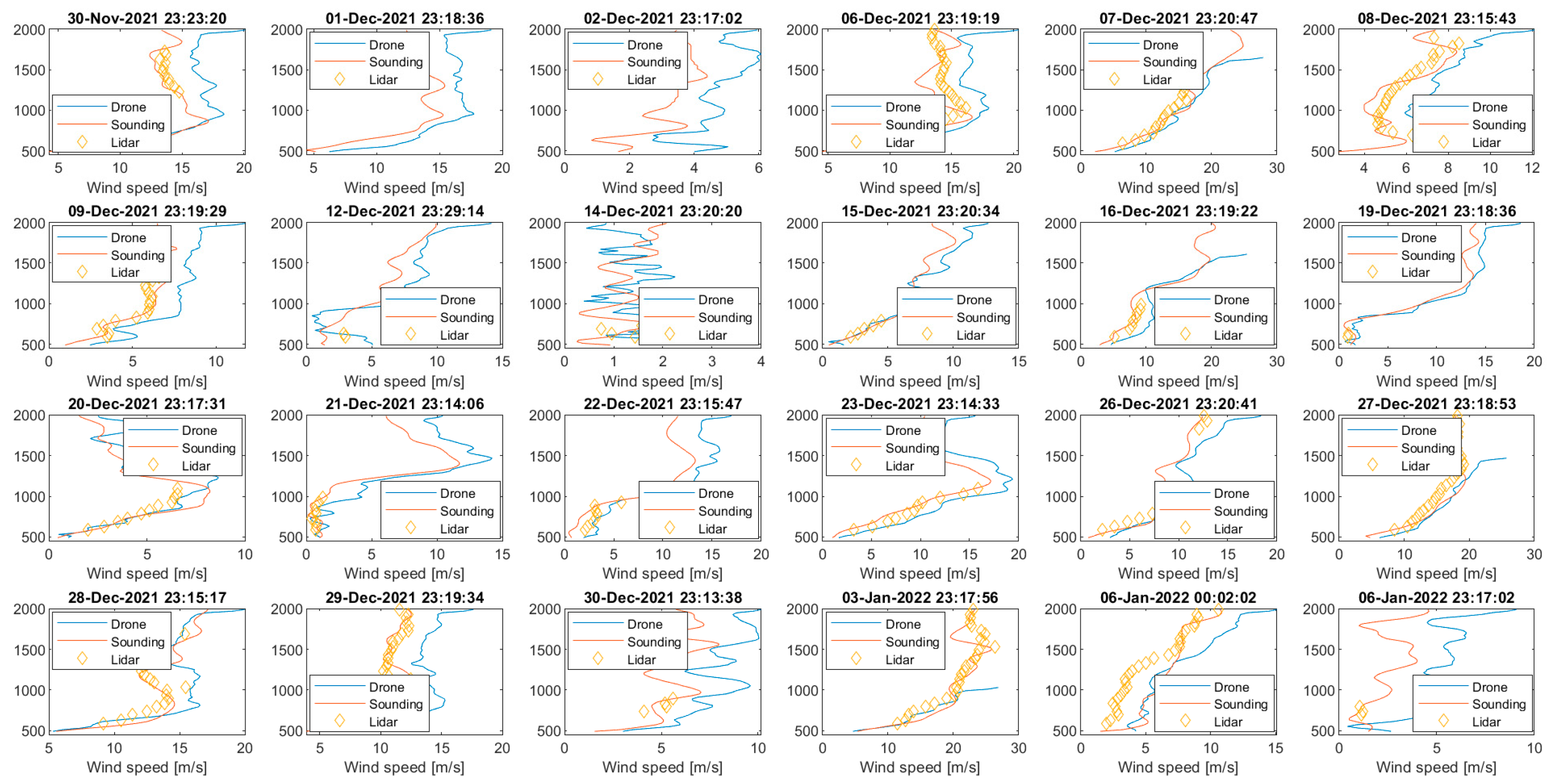
Figure A7.
Wind speed profiles measured above Payerne. Blue: Meteodrone, red: radiosounding, and orange: Doppler LiDAR.
Figure A7.
Wind speed profiles measured above Payerne. Blue: Meteodrone, red: radiosounding, and orange: Doppler LiDAR.
Figure A8.
Distance between the Meteodrone and the radiosonde.
Figure A8.
Distance between the Meteodrone and the radiosonde.
Figure A9.
Upper panels: Difference between the temperatures measured by the Meteodrone and the radiosonde measurements according to the wind speed measured by the radiosonde. Black line: median, shaded area: 25–75% percentile. Lower panel: number of observations in each bin.
Figure A9.
Upper panels: Difference between the temperatures measured by the Meteodrone and the radiosonde measurements according to the wind speed measured by the radiosonde. Black line: median, shaded area: 25–75% percentile. Lower panel: number of observations in each bin.
Figure A10.
Vertical profiles of the specific humidity difference between the Meteodrone and radiosonde measurements (left). Difference between the Meteodrone and radiosonde specific humidity measurements according to the radiosonde measurements (right). Lower panel: number of observations in each bin. Black line: median, shaded area: 25–75% percentile.
References
- Illingworth, A.J.; Cimini, D.; Haefele, A.; Haeffelin, M.; Hervo, M.; Kotthaus, S.; Löhnert, U.; Martinet, P.; Mattis, I.; O’Connor, E.J.; et al. How Can Existing Ground-Based Profiling Instruments Improve European Weather Forecasts? Bull. Am. Meteorol. Soc. 2019, 100, 605–619. [Google Scholar] [CrossRef]
- Leuenberger, D.; Haefele, A.; Omanovic, N.; Fengler, M.; Martucci, G.; Calpini, B.; Fuhrer, O.; Rossa, A. Improving High-Impact Numerical Weather Prediction with Lidar and Drone Observations. Bull. Am. Meteorol. Soc. 2020, 101, E1036–E1051. [Google Scholar] [CrossRef]
- Jensen, A.A.; Pinto, J.O.; Bailey, S.C.C.; Sobash, R.A.; Romine, G.; de Boer, G.; Houston, A.L.; Smith, S.W.; Lawrence, D.A.; Dixon, C.; et al. Assimilation of a Coordinated Fleet of Uncrewed Aircraft System Observations in Complex Terrain: Observing System Experiments. Mon. Weather Rev. 2022, 150, 2737–2763. [Google Scholar] [CrossRef]
- Jensen, A.A.; Pinto, J.O.; Bailey, S.C.C.; Sobash, R.A.; de Boer, G.; Houston, A.L.; Chilson, P.B.; Bell, T.; Romine, G.; Smith, S.W.; et al. Assimilation of a Coordinated Fleet of Uncrewed Aircraft System Observations in Complex Terrain: EnKF System Design and Preliminary Assessment. Mon. Weather Rev. 2021, 149, 1459–1480. [Google Scholar] [CrossRef]
- Pinto, J.O.; O’Sullivan, D.; Taylor, S.; Elston, J.; Baker, C.B.; Hotz, D.; Marshall, C.; Jacob, J.; Barfuss, K.; Piguet, B.; et al. The Status and Future of Small Uncrewed Aircraft Systems (UAS) in Operational Meteorology. Bull. Am. Meteorol. Soc. 2021, 102, E2121–E2136. [Google Scholar] [CrossRef]
- McFarquhar, G.M.; Smith, E.; Pillar-Little, E.A.; Brewster, K.; Chilson, P.B.; Lee, T.R.; Waugh, S.; Yussouf, N.; Wang, X.; Xue, M.; et al. Current and Future Uses of UAS for Improved Forecasts/Warnings and Scientific Studies. Bull. Am. Meteorol. Soc. 2020, 101, E1322–E1328. [Google Scholar] [CrossRef]
- Bärfuss, K.; Dirksen, R.; Schmithüsen, H.; Bretschneider, L.; Pätzold, F.; Bollmann, S.; Panten, P.; Rausch, T.; Lampert, A. Drone-Based Atmospheric Soundings Up to an Altitude of 10 Km-Technical Approach towards Operations. Drones 2022, 6, 404. [Google Scholar] [CrossRef]
- Chilson, P.B.; Bell, T.M.; Brewster, K.A.; Britto Hupsel de Azevedo, G.; Carr, F.H.; Carson, K.; Doyle, W.; Fiebrich, C.A.; Greene, B.R.; Grimsley, J.L.; et al. Moving towards a Network of Autonomous UAS Atmospheric Profiling Stations for Observations in the Earth’s Lower Atmosphere: The 3D Mesonet Concept. Sensors 2019, 19, 2720. [Google Scholar] [CrossRef]
- Samuel, A.C.; Asuquo, P.M.; Ozuomba, S.; Eze, O.C.; Ogbu, C.P. A Review Paper on Unmanned Aerial Vehicles for Vertical. Math. Stat. Eng. Appl. 2023, 72, 924–958. [Google Scholar]
- Whitepaper: How Meteodrones Contribute to Weather Forecasting; Meteomatics: St. Gallen, Switzerland, 2020.
- Bell, T.M.; Greene, B.R.; Klein, P.M.; Carney, M.; Chilson, P.B. Confronting the Boundary Layer Data Gap: Evaluating New and Existing Methodologies of Probing the Lower Atmosphere. Atmos. Meas. Tech. 2020, 13, 3855–3872. [Google Scholar] [CrossRef]
- World Meteorological Organization (WMO). UAS Demonstration Campaign. Available online: https://community.wmo.int/uas-demonstration (accessed on 11 July 2022).
- World Meteorological Organization (WMO). Global Demonstration Campaign for Evaluating the Use of Uncrewed Aircraft Systems in Operational Meteorology: White Paper (WMO-No. 1318); World Meteorological Organization: Geneva, Switzerland, 2023; ISBN 978-92-63-11318-4. [Google Scholar]
- Inoue, J.; Sato, K. Toward Sustainable Meteorological Profiling in Polar Regions: Case Studies Using an Inexpensive UAS on Measuring Lower Boundary Layers with Quality of Radiosondes. Environ. Res. 2022, 205, 112468. [Google Scholar] [CrossRef] [PubMed]
- Koch, S.E.; Fengler, M.; Chilson, P.B.; Elmore, K.L.; Argrow, B.; Andra, D.L.; Lindley, T. On the Use of Unmanned Aircraft for Sampling Mesoscale Phenomena in the Preconvective Boundary Layer. J. Atmos. Ocean. Technol. 2018, 35, 2265–2288. [Google Scholar] [CrossRef]
- Lee, T.R.; Schuyler, T.J.; Buban, M.; Dumas, E.J.; Meyers, T.P.; Baker, C.B. NOAA Air Resources Laboratory Atmospheric Turbulence and Diffusion Division’s Measurements of Temperature, Humidity and Wind Using Small Uncrewed Aircraft Systems to Support Short-Term Weather Forecasting Needs over Complex Terrain. Earth Syst. Sci. Data Discuss. 2022, 1–14. [Google Scholar] [CrossRef]
- Ngan, F.; Loughner, C.P.; Zinn, S.; Cohen, M.; Lee, T.R.; Dumas, E.; Schuyler, T.J.; Baker, C.B.; Maloney, J.; Hotz, D.; et al. The Use of Small Uncrewed Aircraft System Observations in Meteorological and Dispersion Modeling. J. Appl. Meteorol. Climatol. 2023, 62, 817–834. [Google Scholar] [CrossRef]
- De Boer, G.; Diehl, C.; Jacob, J.; Houston, A.; Smith, S.W.; Chilson, P.; Schmale, D.G.; Intrieri, J.; Pinto, J.; Elston, J.; et al. Development of Community, Capabilities, and Understanding through Unmanned Aircraft-Based Atmospheric Research: The LAPSE-RATE Campaign. Bull. Am. Meteorol. Soc. 2020, 101, E684–E699. [Google Scholar] [CrossRef]
- Segales, A.R.; Greene, B.R.; Bell, T.M.; Doyle, W.; Martin, J.J.; Pillar-Little, E.A.; Chilson, P.B. The CopterSonde: An Insight into the Development of a Smart Unmanned Aircraft System for Atmospheric Boundary Layer Research. Atmos. Meas. Tech. 2020, 13, 2833–2848. [Google Scholar] [CrossRef]
- Pillar-Little, E.A.; Greene, B.R.; Lappin, F.M.; Bell, T.M.; Segales, A.R.; de Azevedo, G.B.H.; Doyle, W.; Kanneganti, S.T.; Tripp, D.D.; Chilson, P.B. Observations of the Thermodynamic and Kinematic State of the Atmospheric Boundary Layer over the San Luis Valley, CO, Using the CopterSonde 2 Remotely Piloted Aircraft System in Support of the LAPSE-RATE Field Campaign. Earth Syst. Sci. Data 2021, 13, 269–280. [Google Scholar] [CrossRef]
- Bärfuss, K.B.; Schmithüsen, H.; Lampert, A. Drone-Based Meteorological Observations up to the Tropopause—A Concept Study. Atmos. Meas. Tech. 2023, 16, 3739–3765. [Google Scholar] [CrossRef]
- Barbieri, L.; Kral, S.T.; Bailey, S.C.C.; Frazier, A.E.; Jacob, J.D.; Reuder, J.; Brus, D.; Chilson, P.B.; Crick, C.; Detweiler, C.; et al. Intercomparison of Small Unmanned Aircraft System (SUAS) Measurements for Atmospheric Science during the LAPSE-RATE Campaign. Sensors 2019, 19, 2179. [Google Scholar] [CrossRef]
- Muñoz, L.E.; Campozano, L.V.; Guevara, D.C.; Parra, R.; Tonato, D.; Suntaxi, A.; Maisincho, L.; Páez, C.; Villacís, M.; Córdova, J.; et al. Comparison of Radiosonde Measurements of Meteorological Variables with Drone, Satellite Products, and WRF Simulations in the Tropical Andes: The Case of Quito, Ecuador. Atmosphere 2023, 14, 264. [Google Scholar] [CrossRef]
- Laitinen, A. Utilization of Drones in Vertical Profile Measurements of the Atmosphere. Master’s Thesis, Tampere University, Tampere, Finland, 2019. [Google Scholar]
- Greene, B.R.; Segales, A.R.; Waugh, S.; Duthoit, S.; Chilson, P.B. Considerations for Temperature Sensor Placement on Rotary-Wing Unmanned Aircraft Systems. Atmos. Meas. Tech. 2018, 11, 5519–5530. [Google Scholar] [CrossRef]
- Lee, T.R.; Buban, M.; Dumas, E.; Baker, C.B. On the Use of Rotary-Wing Aircraft to Sample Near-Surface Thermodynamic Fields: Results from Recent Field Campaigns. Sensors 2019, 19, 10. [Google Scholar] [CrossRef] [PubMed]
- Thielicke, W.; Hübert, W.; Müller, U.; Eggert, M.; Wilhelm, P. Towards Accurate and Practical Drone-Based Wind Measurements with an Ultrasonic Anemometer. Atmos. Meas. Tech. 2021, 14, 1303–1318. [Google Scholar] [CrossRef]
- Inoue, J.; Sato, K. Wind Speed Measurement by an Inexpensive and Lightweight Thermal Anemometer on a Small UAV. Drones 2022, 6, 289. [Google Scholar] [CrossRef]
- De Boer, G.; Ivey, M.; Schmid, B.; Lawrence, D.; Dexheimer, D.; Mei, F.; Hubbe, J.; Bendure, A.; Hardesty, J.; Shupe, M.D.; et al. A Bird’s-Eye View: Development of an Operational ARM Unmanned Aerial Capability for Atmospheric Research in Arctic Alaska. Bull. Am. Meteorol. Soc. 2018, 99, 1197–1212. [Google Scholar] [CrossRef]
- Hamilton, J.; de Boer, G.; Doddi, A.; Lawrence, D.A. The DataHawk2 Uncrewed Aircraft System for Atmospheric Research. Atmos. Meas. Tech. 2022, 15, 6789–6806. [Google Scholar] [CrossRef]
- Meteomatics. Weather Forecast with Meteodrones Weather Drones. Available online: https://www.meteomatics.com/en/meteodrones-weather-drones/ (accessed on 14 August 2023).
- Jeannet, P.; Philipona, R.; Richner, H. Swiss Upper-Air Balloon Soundings since 1902. In From Weather Observations to Atmospheric and Climate Sciences in Switzerland: Celebrating 100 Years of the Swiss Society for Meteorology: A Book of the Swiss Society for Meteorology; VDF Hochschulverlag an der ETH Zürich: Zürich, Switzerland, 2016; ISBN 978-3-7281-3745-6. [Google Scholar]
- Jensen, M.P.; Holdridge, D.J.; Survo, P.; Lehtinen, R.; Baxter, S.; Toto, T.; Johnson, K.L. Comparison of Vaisala Radiosondes RS41 and RS92 at the ARM Southern Great Plains Site. Atmos. Meas. Tech. 2016, 9, 3115–3129. [Google Scholar] [CrossRef]
- Philipona, R.; Mears, C.; Fujiwara, M.; Jeannet, P.; Thorne, P.; Bodeker, G.; Haimberger, L.; Hervo, M.; Popp, C.; Romanens, G.; et al. Radiosondes Show That After Decades of Cooling, the Lower Stratosphere Is Now Warming. J. Geophys. Res. Atmos. 2018, 123, 12509–12522. [Google Scholar] [CrossRef]
- World Meteorological Organization. WMO-CIMO Testbed Payerne (Switzerland). Available online: https://community.wmo.int/en/activity-areas/imop/cimo-testbeds-and-lead-centres/Testbed_Switzerland (accessed on 14 August 2023).
- Kumer, V.-M.; Reuder, J.; Furevik, B.R. A Comparison of LiDAR and Radiosonde Wind Measurements. Energy Procedia 2014, 53, 214–220. [Google Scholar] [CrossRef]
- Calpini, B.; Ruffieux, D.; Bettems, J.-M.; Hug, C.; Huguenin, P.; Isaak, H.-P.; Kaufmann, P.; Maier, O.; Steiner, P. Ground-Based Remote Sensing Profiling and Numerical Weather Prediction Model to Manage Nuclear Power Plants Meteorological Surveillance in Switzerland. Atmos. Meas. Tech. 2011, 4, 1617–1625. [Google Scholar] [CrossRef]
- Haefele, A.; Ruffieux, D. Validation of the 1290 MHz Wind Profiler at Payerne, Switzerland, Using Radiosonde GPS Wind Measurements. Meteorol. Appl. 2015, 22, 873–878. [Google Scholar] [CrossRef]
- Löhnert, U.; Maier, O. Operational Profiling of Temperature Using Ground-Based Microwave Radiometry at Payerne: Prospects and Challenges. Atmos. Meas. Tech. 2012, 5, 1121–1134. [Google Scholar] [CrossRef]
- Trzcina, E.; Tondaś, D.; Rohm, W. Cross-Comparison of Meteorological Parameters and ZTD Observations Supplied by Microwave Radiometers, Radiosondes, and GNSS Services. Geod. Cartogr. 2021, 70, e08. [Google Scholar]
- Liu, M.; Liu, Y.-A.; Shu, J. Characteristics Analysis of the Multi-Channel Ground-Based Microwave Radiometer Observations during Various Weather Conditions. Atmosphere 2022, 13, 1556. [Google Scholar] [CrossRef]
- Löhnert, U.; Turner, D.D.; Crewell, S. Ground-Based Temperature and Humidity Profiling Using Spectral Infrared and Microwave Observations. Part I: Simulated Retrieval Performance in Clear-Sky Conditions. J. Appl. Meteorol. Climatol. 2009, 48, 1017–1032. [Google Scholar] [CrossRef]
- Dinoev, T.; Simeonov, V.; Arshinov, Y.; Bobrovnikov, S.; Ristori, P.; Calpini, B.; Parlange, M.; van den Bergh, H. Raman Lidar for Meteorological Observations, RALMO—Part 1: Instrument Description. Atmos. Meas. Tech. 2013, 6, 1329–1346. [Google Scholar] [CrossRef]
- Brocard, E.; Philipona, R.; Haefele, A.; Romanens, G.; Mueller, A.; Ruffieux, D.; Simeonov, V.; Calpini, B. Raman Lidar for Meteorological Observations, RALMO—Part 2: Validation of Water Vapor Measurements. Atmos. Meas. Tech. 2013, 6, 1347–1358. [Google Scholar] [CrossRef]
- Martucci, G.; Navas-Guzmán, F.; Renaud, L.; Romanens, G.; Gamage, S.M.; Hervo, M.; Jeannet, P.; Haefele, A. Validation of Pure Rotational Raman Temperature Data from the Raman Lidar for Meteorological Observations (RALMO) at Payerne. Atmos. Meas. Tech. 2021, 14, 1333–1353. [Google Scholar] [CrossRef]
- Kotthaus, S.; O’Connor, E.; Münkel, C.; Charlton-Perez, C.; Haeffelin, M.; Gabey, A.M.; Grimmond, C.S.B. Recommendations for Processing Atmospheric Attenuated Backscatter Profiles from Vaisala CL31 Ceilometers. Atmos. Meas. Tech. 2016, 9, 3769–3791. [Google Scholar] [CrossRef]
- WMO OSCAR. Application Area: High Res NWP. Available online: https://space.oscar.wmo.int/applicationareas/view/high_res_nwp (accessed on 12 July 2022).
- Haefele, A.; Hervo, M.; Turp, M.; Lampin, J.-L.; Haeffelin, M.; Lehmann, V. The E-PROFILE Network for the Operational Measurement of Wind and Aerosol Profiles over Europe. In Proceedings of the CIMO TECO 2016, Madrid, Spain, 27–29 September 2016. [Google Scholar]
- Gaffard, C.; Li, Z.; Harrison, D.; Lehtinen, R.; Roininen, R. Evaluation of a Prototype Broadband Water-Vapour Profiling Differential Absorption Lidar at Cardington, UK. Atmosphere 2021, 12, 1521. [Google Scholar] [CrossRef]
- Dirksen, R.J.; Sommer, M.; Immler, F.J.; Hurst, D.F.; Kivi, R.; Vömel, H. Reference Quality Upper-Air Measurements: GRUAN Data Processing for the Vaisala RS92 Radiosonde. Atmos. Meas. Tech. 2014, 7, 4463–4490. [Google Scholar] [CrossRef]
- Dirksen, R.J.; Bodeker, G.E.; Thorne, P.W.; Merlone, A.; Reale, T.; Wang, J.; Hurst, D.F.; Demoz, B.B.; Gardiner, T.D.; Ingleby, B.; et al. Managing the Transition from Vaisala RS92 to RS41 Radiosondes within the Global Climate Observing System Reference Upper-Air Network (GRUAN): A Progress Report. Geosci. Instrum. Methods Data Syst. 2020, 9, 337–355. [Google Scholar] [CrossRef]
- Wagner, T.J.; Petersen, R.A. On the Performance of Airborne Meteorological Observations against Other In Situ Measurements. J. Atmos. Ocean. Technol. 2021, 38, 1217–1230. [Google Scholar] [CrossRef]
- Wang, J.; Cole, H.L.; Carlson, D.J.; Miller, E.R.; Beierle, K.; Paukkunen, A.; Laine, T.K. Corrections of Humidity Measurement Errors from the Vaisala RS80 Radiosonde—Application to TOGA COARE Data. J. Atmos. Ocean. Technol. 2002, 19, 981–1002. [Google Scholar] [CrossRef]
Figure 1.
Meteodrone and Meteobase installed at Payerne.
Figure 1.
Meteodrone and Meteobase installed at Payerne.
Figure 2.
Daily number of flights. Only the days when operations were planned are represented.
Figure 2.
Daily number of flights. Only the days when operations were planned are represented.
Figure 3.
Maximum altitude reached by the Meteodrone.
Figure 3.
Maximum altitude reached by the Meteodrone.
Figure 4.
Temperature, relative humidity, and the wind speed and direction profiles above Payerne on 24 May 2022 around 23:00 UTC. Drone measurements are in blue, and the radio sounding is in black. The remote sensing measurements are in red, and the radar wind profiler is in orange. The grey areas represent the spread of the remote sensing measurements between 23:00 and 23:30.
Figure 5.
Temperature, relative humidity, and the wind speed and direction profiles above Payerne on 15 December 2021 around 23:00 UTC. Drone measurements are in blue, and the radio sounding is in black. The remote sensing measurements are in red, and the radar wind profiler is in orange. The grey areas represent the spread of the remote sensing measurements between 23:00 and 23:30.
Figure 6.
Vertical profiles of the difference between the Meteodrone and radiosonde measurements. Left is the temperature, middle is the relative humidity, and right is the wind speed. Black line: median, shaded area: 25–75% percentile.
Figure 6.
Vertical profiles of the difference between the Meteodrone and radiosonde measurements. Left is the temperature, middle is the relative humidity, and right is the wind speed. Black line: median, shaded area: 25–75% percentile.
Figure 7.
Upper panels: the difference between the Meteodrone and radiosonde measurements according to the radiosonde measurements. Left is the temperature, middle is the relative humidity, and right is the wind speed. Black line: median, shaded area: 25–75% percentile. Lower panels: number of observations of each bin.
Figure 8.
Evolution of the RMS of the difference between the radiosondes and Meteodrones (in blue) and remote sensing instruments (in red). Left: temperature, center: specific humidity, right: wind. The WMO requirements for each parameter are represented with dashed lines.
Figure 8.
Evolution of the RMS of the difference between the radiosondes and Meteodrones (in blue) and remote sensing instruments (in red). Left: temperature, center: specific humidity, right: wind. The WMO requirements for each parameter are represented with dashed lines.
Table 1.
Number of flights performed by the Meteodrone.
Table 1.
Number of flights performed by the Meteodrone.
| | # Flights | Complete Nights |
|---|
| Planned | 1024 | 128 |
| Effective | 864 | 87 |
| Effective in % | 75.7% | 68% |
Table 2.
The WMO requirements for high-resolution NWP compared to the drone and remote sensing performances for the temperature, humidity, and wind profiles.
Table 2.
The WMO requirements for high-resolution NWP compared to the drone and remote sensing performances for the temperature, humidity, and wind profiles.
| | Goal | Breakthrough | Threshold | Drone | Remote Sensing |
|---|
| Atmospheric temperature | 0.5 K | 1 K | 3 K | 0.68 K | 0.72 K | Microwave radiometer |
| Specific humidity | 2% | 5% | 10% | 8.3% | 9.2% | RALMO |
Wind
(horizontal) | 1 m.s−1 | 2 m.s−1 | 5 m.s−1 | 3.1 m.s−1 | 1.8 m.s−1 | Wind
LiDAR |
| Disclaimer/Publisher’s Note: The statements, opinions and data contained in all publications are solely those of the individual author(s) and contributor(s) and not of MDPI and/or the editor(s). MDPI and/or the editor(s) disclaim responsibility for any injury to people or property resulting from any ideas, methods, instructions or products referred to in the content. |
© 2023 by the authors. Licensee MDPI, Basel, Switzerland. This article is an open access article distributed under the terms and conditions of the Creative Commons Attribution (CC BY) license (https://creativecommons.org/licenses/by/4.0/).


 ,
, 


