The Influence of Meteorology Initialization on Ozone Forecasting in the Great Lakes Region during MOOSE Study

Abstract

This study investigates the influence of meteorology initialization on surface ozone prediction in the Great Lakes region using Canada’s operational air quality model (GEM-MACH) at a 2.5 km horizontal resolution. Two different initialization techniques are compared, and it is found that the four-dimensional incremental analysis updating (IAU) method yields improved model performance for surface ozone prediction. The IAU run shows better ozone regression line statistics (y = 0.7x + 14.9, R² = 0.2) compared to the non-IAU run (y = 0.6x + 23.1, R² = 0.1), with improved MB and NMB values (3.9 ppb and 8.9%, respectively) compared to the non-IAU run (4.1 ppb and 9.3%). Furthermore, analyzing ozone prediction sensitivity to model initialization time reveals that the 18z initialization leads to enhanced performance, particularly during high ozone exceedance days, with an improved regression slope of 0.9 compared to 0.7 for the 00z and 12z runs. The MB also improves to −0.2 ppb in the 18z run compared to −2.8 ppb and −3.9 ppb for the 00z and 12z runs, respectively. The analysis of meteorological fields reveals that the improved ozone predictions at 18z are linked to a more accurate representation of afternoon wind speed. This improvement enhances the transport of ozone, contributing to the overall improvement in ozone predictions.

1. Introduction

High concentrations of surface ozone (O₃) and the frequent violation of air quality standards have long been recognized as significant air quality and public health concerns in the Great Lakes region [1,2]. The unique combination of emissions from human activities and the meteorological conditions influenced by the presence of the lakes contribute to the elevated ozone levels observed in both side of the lakes, in Canada and the Unites States [3,4,5,6,7].

To address the shared concerns in this special border region and gain a better understanding of the factors contributing to high ozone levels, several field studies have been conducted aiming to collect meteorological and chemical measurements. Two earlier examples are the Lake Michigan Ozone Study (LMOS) [8] and the Program for Research on Oxidants: Photochemistry, Emissions, and Transport (PROPHET) [9], and the most recent one is the Michigan–Ontario Ozone Source Experiments (MOOSE) field campaign conducted in summer 2021 [10].

Complementary to field studies, Chemical Transport Models (CTMs) and data-based machine learning methods [11,12] have been widely used to enhance understanding of ozone formation and transport processes. Despite significant advancements in models, the prediction of ozone, especially during high ozone episodes, remains a challenging problem, particularly in complex coastal regions where local emissions, transport processes, and meteorological conditions interact in complex ways [13,14,15,16].

Due to the intricate interplay of various processes, accurate air quality forecasts heavily depend on the output from numerical weather prediction (NWP) models. To achieve precise predictions of ozone concentrations, it is essential to have a comprehensive understanding of the meteorological factors that influence ozone formation and transport. Therefore, a proper representation of these meteorological factors in the models is crucial.

In recent years, advancements in meteorological data assimilation techniques have shown promise in improving the accuracy of NWP forecasts mainly through correcting errors in the initial conditions of the model. Among many, the four-dimensional Incremental Analysis Update (IAU) technique [17], is one of the advanced methods used in model initialization. This method allows a gradual incremental update of the observation into the system and thus minimizes the dynamics and thermodynamic imbalances related to the model initialization in the model. At Environment and Climate Change Canada (ECCC), Dorval, QC, Canada, the four-dimensional IAU technique was implemented in the global NWP operational system in fall 2014 [18], replacing the previous initialization method based on the full-field digital filter [19,20]. Since then, other operational systems, including the regional and national ones, have also upgraded to this method. Recently in July 2021, during the MOOSE field study, the operational high-resolution deterministic prediction system at ECCC upgraded its initialization method to IAU technique as part of the 3rd official ECCC’s innovations cycle [21].

Several studies showed an improvement in the model performance for meteorological prediction by using IAU [22,23,24]. However, the impact of these improved initialization techniques on ozone predictions, especially during high ozone episodes, remains to be understood.

Moreover, while a handful of studies have delved into assessing the sensitivity of NWP model skills in the context of initialized forecast start cycles [25,26], a significant gap remains in understanding the potential implications of these sensitivity findings for ozone prediction.

The main objective of this study is to investigate the sensitivity of surface ozone to meteorological initialization. To achieve this, we aim to address the following key questions: (1) What is the impact of changing the meteorological initialization from the non-IAU (digital filter) method to the four-dimensional IAU technique on ozone concentration? (2) Does the initialization forecast cycle time of the model have an impact on the predictive skill for ozone? (3) Is the sensitivity of ozone to initialization time different for high ozone episodes compared to normal ozone days? (4) Which meteorological parameter exhibits the highest sensitivity to initialization and has more consequent impact of ozone response? By addressing these questions, this study aims to enhance our understanding of the relationship between meteorology and surface ozone, and provide insights for improving ozone predictions in the future.

In the following sections, we will provide a detailed description of the air quality model used, including the emissions and observational data employed in our study. We will then proceed to discuss the results on the impact of initialization with IAU and the influence of initialization time on ozone prediction. Finally, we will conclude by summarizing the key findings derived from our analysis.

2. Materials and Methods

2.1. Model Description

The air quality model used in this study was the version 3.0 of the ECCC Global Environmental Multiscale-Modelling Air-Quality and Chemistry (GEM-MACH) model. GEM-MACH is an online, one-way coupled chemical transport model that incorporates a detailed representation of atmospheric chemistry including emissions, dispersion and removal processes, within the GEM atmospheric model, an ECCC’s operational global and regional numerical weather prediction model [27,28,29,30]. The GEM-MACH model has been used operationally by ECCC for regional air quality forecasting since 2009 [31,32,33]. More detailed description of the multi-phase chemistry representations of GEM-MACH including the gas-, aqueous-, and particle-phase and an evaluation of its performance for common air pollutants appears in [32,34,35,36,37].

In this study, a high-resolution limited-area model (LAM) configuration of GEM-MACH with an urban canopy model based on Town Energy Balance (TEB) scheme was used. More description can be found in [38,39,40,41,42]. The initial surface variables are provided by a 2.5 km Canadian Land Data Assimilation System (CaLDAS) coupled with GEM NWP model [43].

The Canadian anthropogenic emissions data are based on the 2015 national Air Pollutant Emissions Inventory (APEI) projected to 2020 [44], accounting for projected changes in population, economic activity, and the energy use over the 5 years, from 2015 to 2020, as well as the implementation over this period of already-legislated air pollution control measures and expected facility openings or closures. The US anthropogenic emissions data comes from a projected 2023 US National Emissions Inventory (NEI), which is based on the 2016 US NEI. The point sources are based on the 2018 NEI emissions. This emission dataset is obtained from version 1 of the US Environmental Protection Agency (EPA), Washington, DC, USA, Air Emissions Modeling Platform for policy development application [45]. The national emissions inventories were processed using version 3.7 of the Sparse Matrix Operating Kernel Emissions (SMOKE) tool [46] to generate model-ready hourly emissions. Large stacks with heights greater than 15 m are considered as major point sources, for which the plume rise is calculated in the GEM-MACH model. The hourly gridded emissions were generated for a representative week of each month; thus, they vary by hour of the day, day of the week, and month of the year.

2.2. Simulations Setup

The forecast domain covers Southern Ontario and a significant portion of the northeastern United States, which includes four major urban cities: Toronto, Chicago, New York City, and Detroit (red box domain in Figure 1). This domain is commonly known as ‘Pan Am’ as it was initially created for high-resolution air quality modelling purposes during the 2015 Pan American Games in Ontario [47]. The model grid is a rotated latitude–longitude map projection with 2.5 km horizontal grid spacing and a hybrid sigma-pressure coordinate with a Charney–Phillips staggered vertical grid, with 62 levels from the surface to 10 hPa.

Figure 2 presents a flowchart of the main components of the simulations setup used in this study. Hourly meteorological boundary conditions are from the high-resolution 2.5 km GEM operational meteorological forecasts. Chemical lateral boundary conditions were piloted using 10 km regional GEM-MACH model simulations. The chemical tracers are initialized using 10 km simulations only at the beginning of the first cycle. For subsequent cycles, the initial chemical fields came from the final forecast fields of the previous run (i.e., from the end of the 24 h cycle). The meteorological fields are initialized at the beginning of each integration cycle. Two different initialization methods were employed for the meteorological fields in the simulations conducted in this study. The first method is the four-dimensional IAU, where the 4D analysis increments derived from the Ensemble Variational (EnVar) approach are gradually incorporated into the model over a 6 h window, extending from $\mathrm{T}-3 \mathrm{h}$ to $\mathrm{T}+3 \mathrm{h}$. This incremental update ensures a smoother transition and minimizes the dynamics and thermodynamic imbalances associated with model initialization. The second method, known as the digital filter (hereafter referred to as the non-IAU), applies a single full-field analysis at the initial time to adjust the model’s meteorological variables.

The simulations conducted in this study utilized the operational configuration of the GEM-MACH model. It is noteworthy that this configuration was also employed by ECCC during the MOOSE field campaign to generate real-time simulations. These simulations were subsequently provided to the field measurement teams as daily briefings, enabling them to strategically position their mobile equipment for effective capture of ozone plumes. While the MOOSE study period primarily covered a period from 20 May to the end of June 2021, the simulation period considered for this study started from 19 June and extended to 31 August 2021. This duration was selected primarily due to the availability of IAU data, which became accessible on 19 June 2021, coinciding with the initiation of parallel runs as part of the 3rd innovation cycle implemented in the main operational ECCC’s NWP models in summer 2021.

Two distinct sets of simulations were designed for this study. The first set involves simulations initialized at 00z, used for comparing the performance of the IAU against the non-IAU method. The second set of simulations focus on the IAU initialization technique with varied initialization times to include runs at 00z, 12z, and 18z. By examining these different sets of simulations, the study aimed to assess the impact of the initialization method and time on the accuracy of ozone predictions.

2.3. Observations

Hourly measurements for surface O₃ concentrations for Canada were obtained from provincial and municipal air quality monitoring networks that are part of the larger National Air Pollution Surveillance (NAPS) Program [48]. Measurements for the US were obtained from the EPA Air Quality System (AQS) [49]. The measurements are transmitted either directly to Environment and Climate Change Canada (ECCC) or indirectly via the US Environmental Protection Agency’s AirNow system (https://docs.airnowapi.org/) (accessed on 30 August 2023). Hourly meteorological measurements including the temperature at 2 m above the surface and wind speed and direction at 10 m were obtained from the National Climate Data and Information Archive (https://climate.weather.gc.ca/) (accessed on 30 August 2023) for Canada and from the Clean Air Status and Trends Network (CASNET) for the US (https://www.epa.gov/castnet) (accessed on 30 August 2023).

While the simulation domain encompasses a wide area of southeastern Canada and northeastern USA, this study focuses only on the measurements within a specific subset of that domain. Specifically, the analysis concentrates on the Ontario/Michigan border region and the densely populated Toronto area. The study analysis domain is shown as a red box in Figure 3. This figure shows the location of measurement monitoring stations for ozone marked as green triangles and meteorology stations marked as red triangles. A total number of 63 monitoring stations for ozone and 72 for meteorology are considered in analysis presented in next sections of this study.

We calculated the maximum daily 8 h average (referred to as MDA8) from the observed hourly surface ozone data. For the analysis presented in the next sections, observation datasets are divided into two separate categories. The first category includes the days associated with exceedance of the 2024 Canadian Air Quality Standard (CAAQS) which are the days with MDA8 greater than 60 ppb, (referred to as ‘exceedance days’). The second category includes the days not associated with the exceedance of the CAAQS (referred to as ‘non-exceedance days’). This allows us to assess the impact of initialization on the high ozone episodes.

3. Results and Discussion

3.1. Impact of IAU Initialization

In order to assess the impact of upgrading the initialization technique in operational implementation of GEM-MACH from a single-time full-field digital filter to the four-dimensional IAU, two sets of simulations were performed and compared in this section. Figure 4a displays the mean observed surface MDA8 ozone concentration (depicted in green) along with the model predictions for simulations using the IAU initialization employed (shown in blue) and the non-IAU initialization (shown in gray), both initialized at 00z. The first set of bar columns in this figure represents the values averaged over the entire simulation period across all ozone monitoring stations located inside the red box in Figure 3. Overall, the model overestimates the observed mean MDA8 ozone concentration (45.1 ppb) in both the IAU (48.6 ppb) and non-IAU (48.7 ppb) runs. The difference between the two model runs is minimal, with a marginal deviation of only 0.1 ppb when considering all stations and days collectively.

To further evaluate the impact of IAU, we specifically examined high ozone episodes in comparison to normal conditions. The average MDA8 is presented separately for exceedance and non-exceedance cases, shown in the middle and right set of column bars in Figure 4a. The model values for non-exceedance cases are 47.7 ppb for the IAU run and 47.9 ppb for the non-IAU run, both overestimating the observed MDA8 (43.8 ppb). As expected, for exceedance cases, the average observed MDA8 is higher compared to the non-exceedance average, with a substantial margin of 21 ppb. Unlike the non-exceedance cases, the model tends to underestimate the average MDA8 ozone concentration for both the IAU run (62 ppb) and the non-IAU run (61.7 ppb). For both exceedance and non-exceedance cases, the IAU run demonstrated a slight improvement over the non-IAU run.

The scatter plots in Figure 4b,c illustrate the comparison between observed surface MDA8 ozone concentrations and model predictions for IAU (blue points) and non-IAU (gray points) runs, respectively. The statistical metrics such as mean bias (MB), normalized mean bias (NMB) and root mean square error (RMSE) are also presented in this figure. While MB, NMB and RMSE provide valuable information about the accuracy and bias, the regression equation and correlation coefficient quantify the relationship between predicted and observed values. To provide a visual reference, a vertical dashed red line is included in these figures, representing the 60 ppb CAAQS threshold for observed MDA8 ozone. This line serves to distinguish non-exceedance cases (shown in lighter points) on the left side of the line from exceedance cases (shown in darker points) on the right side. Consistent with the pattern observed in Figure 4a, the regression line, MB, and NMB reveal an overestimated trend when the observed MDA8 ozone concentration is below the 60 ppb threshold, while underestimation occurs during ozone exceedance events.

For both cases, the IAU run consistently demonstrated a better overall performance compared to the non-IAU run, as evidenced by the statistical metrics and the regression equations. On exceedance days, the IAU run showed improved statistics for the ozone regression line (y = 0.7x + 14.9, R² = 0.2) compared to the non-IAU run (y = 0.6x + 23.1, R² = 0.1). Additionally, the IAU run exhibited better MB and NMB values (−2.8 ppb and −4.4%, respectively) compared to the non-IAU run (−3.0 ppb and −4.7%, respectively). For non-exceedance days, the IAU run also displayed an enhanced slope of the regression line (0.8) compared to the non-IAU run (0.7). The MB and NMB values further improved from 4.1 ppb and 9.3% in the non-IAU run to 3.9 ppb and 8.9% in the IAU run. These consistent improvements in statistical performance highlight the importance of utilizing the IAU technique to enhance surface ozone predictions.

To explore potential factors contributing to the improved model performance associated with the IAU initialization, we examined the model performance in key meteorological parameters.

Table 1. Statistical indices for daylight (7:00 A.M.–8:00 P.M.) 2 m temperature and 10 m wind speed and direction predicted by the model versus observations.

		Mean	Standard Deviation (SD)	Mean Bias	NMB (%)	RMSE
Temperature (°C)	Obs	21.96	4.46
	IAU	21.99	4.45	0.03	0.16	2.10
	Non-IAU	22.01	4.43	0.06	0.27	2.10
Wind speed (m/s)	Obs	3.16	1.89
	IAU	3.09	1.69	−0.11	−3.46	2.06
	Non-IAU	3.07	1.68	−0.12	−3.91	2.05
Wind direction (degree)	Obs	207.50	96.32
	IAU	204.96	95.26	−1.50	−0.72	130.19
	Non-IAU	204.62	95.35	−1.82	−0.88	130.31

presents the statistical indices including the mean values, standard deviation, MB, NMB and RMSE for daylight temperature at 2 m above the surface, as well as wind speed and direction at 10 m above the surface, to facilitate comparisons of results between IAU and non-IAU cases.

The model demonstrates good performance in predicting the mean daylight temperature, as evidenced by the close agreement between the predicted values for both IAU (21.99 °C) and non-IAU (22.01 °C) and the observed value of 21.96 °C. The minimal mean biases (0.03 °C for the IAU and 0.06 °C for the non-IAU run), combined with NMB values below 1%, indicate a high level of accuracy for both cases. Additionally, considering the mean and standard deviation, the model predictions exhibit precision as they fall within one standard deviation of the observed values. Comparatively, the IAU run exhibits better accuracy for temperature as indicated by MB and NMB values lower than those of the non-IAU run.

In terms of wind speed, the observed daylight mean value is a moderate 3.16 m/s. The model predicted values for both the IAU (3.09 m/s) and non-IAU (3.07 m/s) runs closely correspond to the observed value. There is an overall minor underestimation, with mean biases of −0.11 m/s and −0.12 m/s for the IAU and non-IAU runs, respectively. However, there is a slight improvement in statistics observed in the IAU run compared to the non-IAU run, with NMBs of −3.5% and −4%, respectively.

Both runs predict a wind direction of West-Southwest (approximately 205 degrees), whereas the observed wind direction is closer to South-Southwest (approx. 207 degrees). Despite relatively high standard deviations (96 degrees), signifying notable variability in wind direction, the model’s mean value remains within one standard deviation of the observed values. This alignment, along with a low NMB (below −1%), suggests a commendable performance by the model. Similar to the wind speed, there are slightly improved biases for the IAU run compared to the non-IAU.

Overall, the statistical evaluations of the temperature and wind fields, which are the two main meteorological factors influencing ozone, demonstrate a modest yet noteworthy improvement when the IAU technique is employed for model initialization. These improvements could contribute to better ozone concentration prediction performance that is obtained when this technique is used.

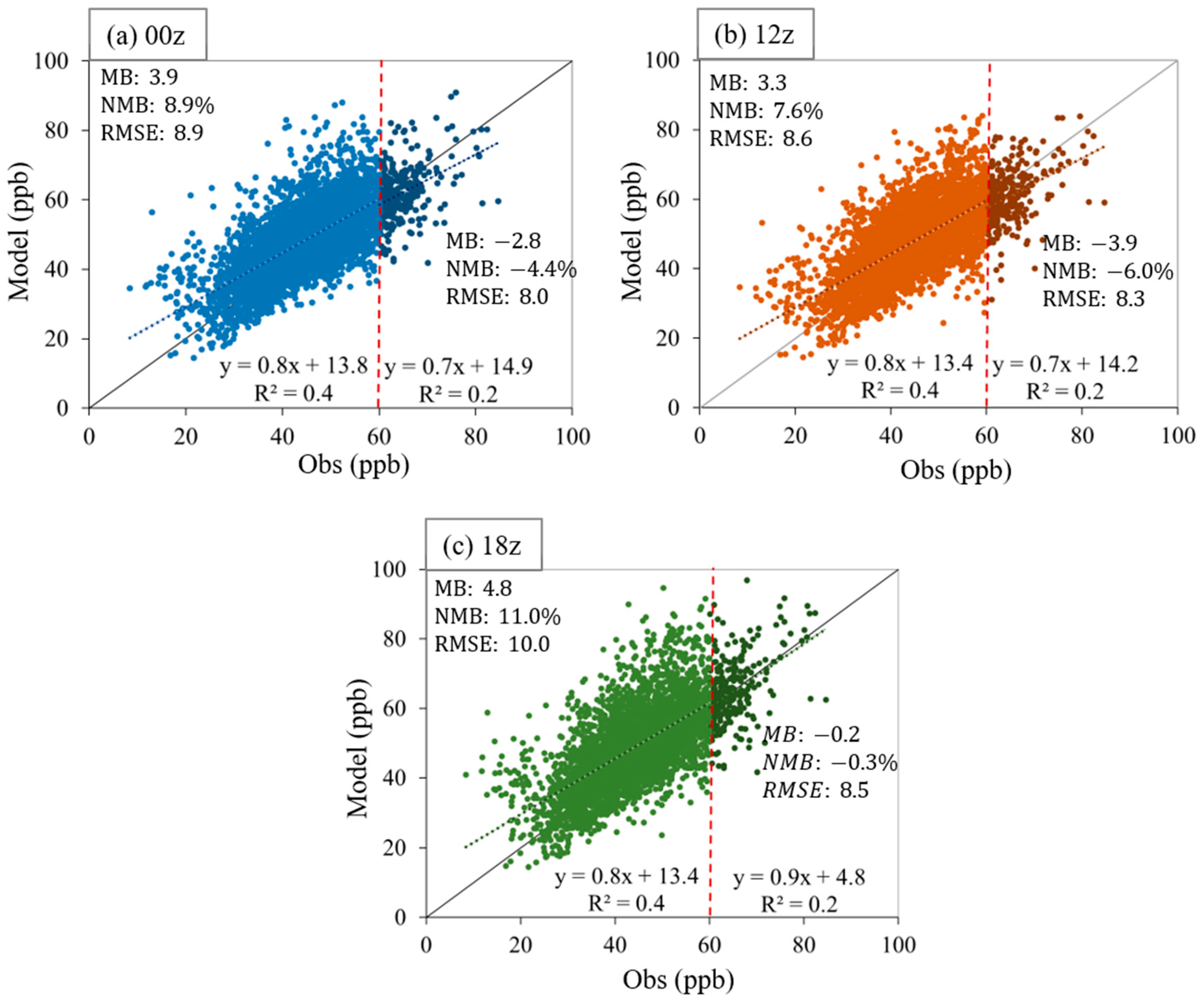
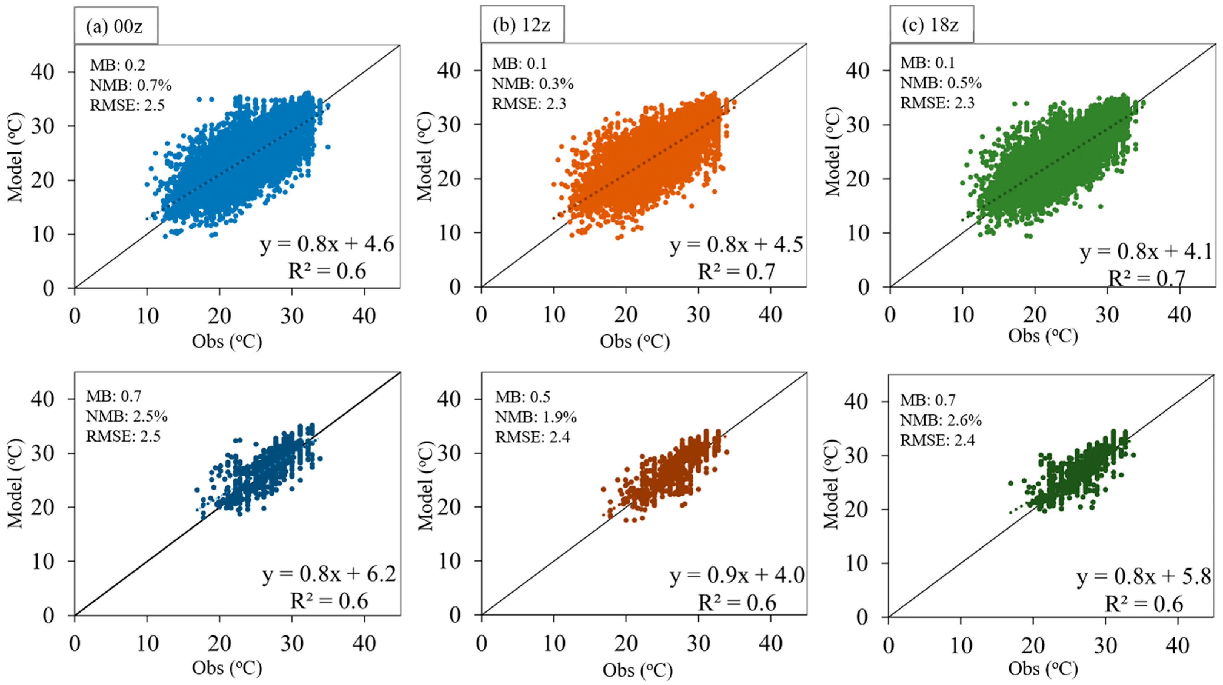
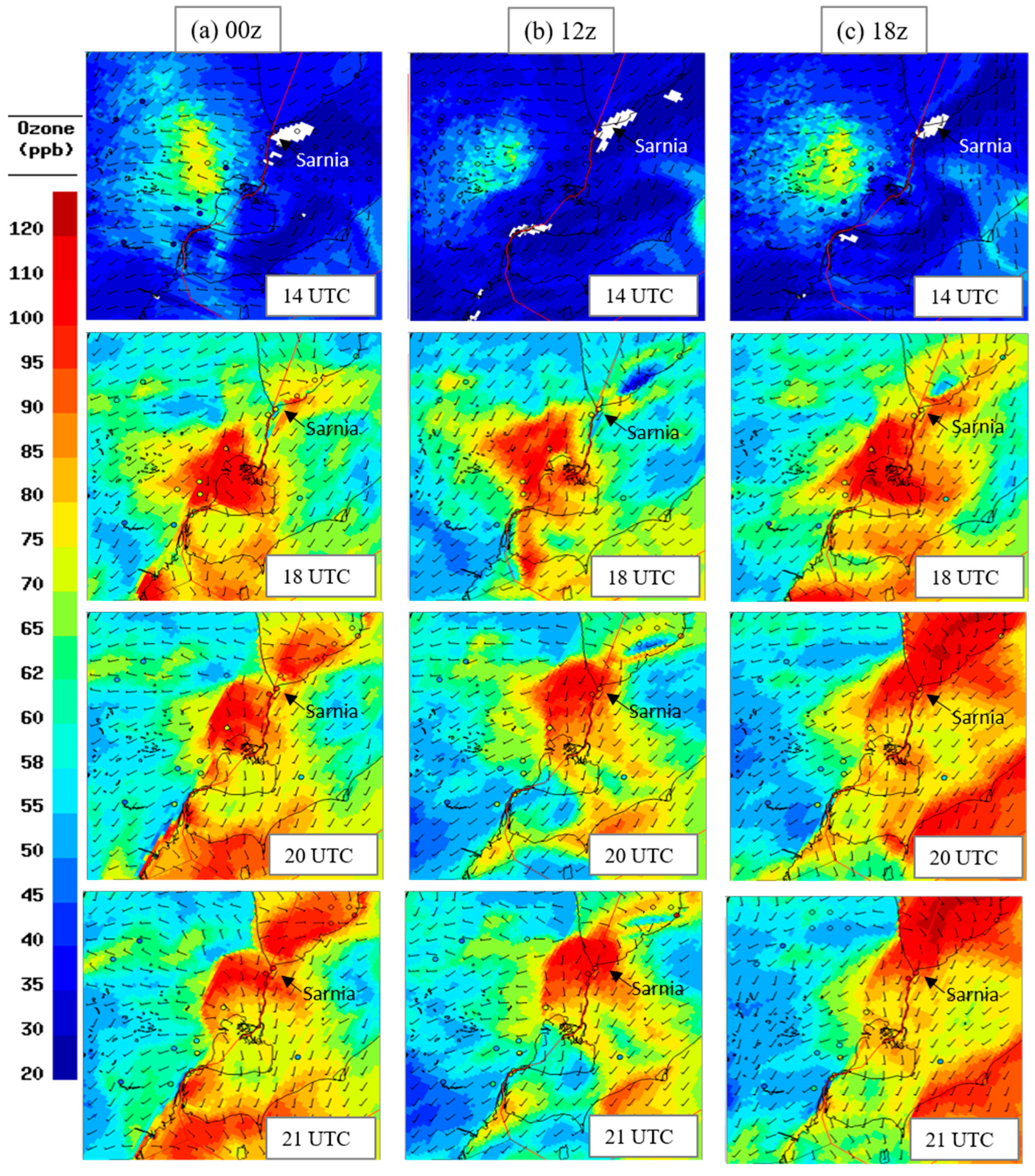
3.2. Impact of Initialization Time

To assess the influence of initialization time on the performance of the model, we conducted a comparative analysis of three simulations that are initialized at different times of the day. These simulations employed the IAU technique for initialization and used identical model configurations, with the sole distinction being the starting time of the model. It is important to note that during the initialization phase, only the surface meteorology fields were assimilated, while the chemistry fields at initial time were copied from the last hour of the previous run cycle.

Figure 5 presents scatter plots of observed surface MDA8 ozone concentrations plotted against the corresponding model-predicted values for three different simulations initialized at 00z (Figure 5a), 12z (Figure 5b), and 18z (Figure 5c). Similar to Figure 4, a vertical line indicating the CAAQS threshold is included to differentiate non-exceedance cases (depicted in lighter points) on the left side of the line from exceedance cases (depicted in darker points). In all three cases, the scatter plots exhibit a trend line positioned above the 1:1 line for non-exceedance cases, indicating an overestimation of the model compared to the observed surface MDA8 ozone. Conversely, in exceedance cases, the trend line is situated below the 1:1 line, suggesting an underestimation of the model. When evaluating the statistics for cases when the observed ozone concentration falls within the CAAQS limit (non-exceedance represented by lighter points), we observed consistent regression equations and correlations among all three runs. However, the 18z run shows higher overestimation of ozone for non-exceedance cases, as evidenced by increased MB, NMB, and RMSE values. However, the 18z run demonstrates a superior performance in predicting exceedance cases compared to the other two runs, with a greater slope of 0.9, compared to 0.7 for the 00z and 12z runs. Notably, there is also a significant improvement in MB and NMB for the 18z run. The MB is −0.2 in the 18z run, which is better than −2.8 and −3.9 in the 00z and 12z runs, respectively. Similarly, the NMB of −0.3% in the 18z run is superior to the −4.4% and −6% in the 00z and 12z runs, respectively. These findings suggest that initializing the model later in the afternoon (at 18z, 2:00 P.M. local time) enhances the model’s ability to predict surface ozone and, in particular, high ozone episodes.

In order to explore a possible connection with meteorology, the meteorological fields, including temperature and wind speed are examined for three initialization times. As the monitoring stations for meteorology and ozone may not be collocated, a simplified pairing approach was employed to establish a relationship for exceedance ozone cases. By matching the meteorology and ozone stations based on their proximity, the associated meteorology station was identified as an exceedance station for days when the ozone levels surpassed the CAAQS threshold. In the statistical meteorological analysis in this section, we focused only on the hours from 1 P.M. to 8 P.M., referred to as the ‘afternoon period’, which typically corresponds to the time when peak ozone concentrations typically occur during the summer.

Figure 6 and Figure 7 illustrate the scatter plots between the observed and model-predicted 2 m temperatures and 10 m wind speeds during the afternoon for three different initialization times. The top panels represent non-exceedance cases (light colors), while the bottom panels depict exceedance cases (dark colors).

The statistical metrics (MB and NMB) for temperature predictions (Figure 6) indicate a slight positive bias, with a maximum error of 0.7 °C (2.6%), suggesting a tendency to overestimate afternoon temperature across all three runs. Among them, the 12z run demonstrates a relatively better performance under during non-exceedance and exceedance days, as indicated by lower MB and NMB values, compared to the other two runs. The slope of the regression line is improved to 0.9 for the 12z run for exceedance days. Overall, the 12z run consistently outperforms the other two runs in terms of temperature prediction. However, it is important to note that, as illustrated in the previous figures, the 18z run consistently demonstrates superior performance in predicting ozone levels. This intriguing finding implies that the model’s enhanced ability to predict ozone in the 18z run may not be directly attributed to the accuracy of temperature predictions.

Regarding the wind speed (Figure 7), the model tends to underestimate, as indicated by the negative MB and NMB values across all data points. The underestimation is relatively lower for the 18z run compared to the 00z and 12z runs, as reflected in improved MB and NMB values for both non-exceedance and exceedance days in this run. The NMB of −10% in the 18z run was better than the −16% in the 00z run on exceedance days. Consistently, the 18z run shows a slightly stronger regression slope (0.5) when compared to the 00z and the 12z runs (0.4). This consistent pattern aligns with the superior performance of the 18z model run in ozone prediction, particularly for high exceedance values. These findings suggest a potential link between the improved representation of wind speed in the 18z run and its enhanced ability to predict ozone, especially during periods of high exceedance. The more accurate depiction of wind speed in the 18z run likely contributes to a better reflection of ozone transport and dispersion, thus leading to improved ozone predictions during critical episodes.

To further analyze the impact of initialization time on the diurnal variation of ozone and meteorology, the average diurnal time series were compared for two cases in Figure 8. The observed diurnal time-series for surface ozone concentrations (Figure 8a) show distinct differences between days of exceedance and non-exceedance, especially regarding the peak times. During the non-exceedance days, the peak ozone concentration occurs during the midday, around 3–4 P.M. However, for exceedance days, a bimodal diurnal pattern is evident, with one maximum during the midday hours and an additional higher peak in early evening, around 8 P.M. As expected, ozone concentrations are generally higher throughout the entire day for exceedance days. Interestingly, the minimum ozone concentration observed in the early morning, around 7 A.M, is higher for exceedance days, suggesting a potential accumulation of ozone from prior afternoon ozone production and light circulating winds overnight, a phenomenon previously addressed by other studies [50].

The diurnal time-series of temperature (Figure 8b) and wind speed (Figure 8c) are positively correlated with the ozone diurnal variations. On exceedance days, higher temperatures and increased wind speeds are commonly observed, indicating favorable meteorological conditions that facilitate ozone formation and transport. The model tends to overestimate ozone concentrations during the afternoon hours (1:00 to 7:00 P.M.) across all three model runs, especially on non-exceedance days. This can be partially attributed to the model’s tendency to predict higher temperature and lower wind speed during this time period, which creates favorable conditions for ozone production and accumulation (i.e., slower transport). This behavior of the model has improved in the ozone plots for exceedance days, where the 18z run outperforms the other two runs in detecting the observed early evening peak ozone and continues to show superior performance during nighttime. This improvement is primarily associated with the 18z run’s improved representation of wind speed (Figure 8c), as temperature still exhibits overestimation during the afternoon for exceedance cases. It is interesting to note that the three model runs exhibit similar behaviors for non-exceedance days, suggesting a limited impact of initialization time on meteorology variables and ozone concentrations under such conditions. However, significant differences emerge among the model runs during exceedance days, with the 18z run demonstrating superior performance, particularly in capturing wind speed and ozone concentration. This highlights the heightened sensitivity of high ozone episode predictions to changes in the model’s initialization time, primarily attributed to the improved representation of wind speed in the 18z run.

A case study of a high ozone day observed in Sarnia, Ontario, on 24 August 2021 was selected for analysis. Sarnia is situated in southwestern Ontario, positioned directly on the Canadian border with the United States and adjacent to Port Huron, Michigan. The time series for surface ozone, temperature, and wind speed for this particular day in Sarnia is shown in Figure 9. The observed surface ozone concentration for this particular day (Figure 9a) exhibited an upward trend from the early morning hours, reaching its first peak of 73 ppb at 1 P.M. After a slight decrease, it continued to rise, reaching a second maximum value of 97 ppb at around 5 P.M. This late afternoon peak ozone can mainly attributed to the time needed to accumulate ozone during the day, as supported by findings from other previous studies [51,52]. The three model runs displayed distinct patterns during the daytime and in terms of the peak ozone times. The 12z run performs better in capturing the observed main peak at 5 P.M. However, it tends to consistently underestimate ozone concentrations in the preceding hours, particularly missing the first maximum. The peak times for ozone in the three model runs occurred at different times, which aligns with the wind speed patterns. Specifically, the 00z run predicted lower wind speed, resulting in slower transport rates compared to the other two runs and the observed data.

Figure 10 displays the spatial distribution of the surface ozone field over the Michigan–Ontario border region on 24 August 2021, at various hours of the afternoon (14, 18, 20, and 21 UTC), allowing comparison among the results from three different initialization times. At 14 UTC, all three runs show a plume of ozone traveling from north Detroit toward Lake St.Clair. At 18 UTC, a lake breeze forms to the west of the lake, converging with southwesterly wind, resulting in maximum ozone concentration predicted at the convergence front. This ozone-rich air mass then moves toward the north and northeast, reaching Sarnia at 20 UTC and 21 UTC.

The movement speed of the air mass varies among the three model runs, with the 18z run showing a faster movement of the plume and the 00z run being the slowest. Notably, the 18z run accurately captures the high ozone levels observed in Sarnia, at 20 UTC and 21 UTC, outperforming the other two runs. Additionally, the 18z run demonstrates better prediction of high ozone values observed in Grand Bend, at 21 UTC. It is interesting to note the overestimation of ozone at 20 and 21 UTC in the back of the plume for the 00z and 12z runs at the New Haven station, located northwest of Lake St. Clair in Michigan. This overestimation can be attributed to the slower movement of the ozone plume in the 00z and 12z runs, in contrast to the 18z run, which accurately captures the observed ozone values throughout the plume’s trajectory. The 18z run demonstrates superior performance in reproducing ozone levels both near the leading edge and at the trailing end of the plume, leading to more precise representation of ozone concentrations along its entire path.

4. Summary and Conclusions

This study aimed to investigate the influence of meteorology initialization on surface ozone prediction in the Great Lakes region using the operational GEM-MACH model at a horizontal resolution of 2.5 km. The simulations were performed over a period from 19 June to 31 August 2021, corresponding to the extended MOOSE field campaign conducted in the summer of 2021. The analysis was conducted separately for two types of days: exceedance days, representing days in which observed ozone levels exceeded Canada’s CAAQS 2024 threshold (60 ppb), and non-exceedance days. The evaluation of the model’s performance against observations for these two types of days revealed distinct patterns. During normal non-exceedance ozone days, the model tended to overestimate surface ozone concentrations, while on exceedance days, it showed underestimation.

The first part of the analysis focused on comparing the ozone predictions between two different meteorology initialization techniques implemented in consecutive versions of the operational high-resolution NWP model at ECCC: the four-dimensional IAU method and the conventional single-time, full-field digital filter. The comparison of statistical indices (MB, NMB, and RMSE) and regression equations showed improved model performance for surface O₃ for both exceedance and non-exceedance days when the IAU technique was employed compared to when it was not used. Consistent with this, the statistical evaluation of key meteorological parameters, such as daylight 2 m temperature and 10 m wind field, also demonstrated enhanced model predictions for meteorology when the IAU approach was employed for model initialization. These findings underscore the importance of employing advanced meteorology initialization techniques to enhance the overall forecasting capabilities of NWP models for applications in air quality and meteorology.

Moreover, this study highlights the link between the accuracy of meteorological parameters achieved through the IAU initialization technique and the subsequent performance of the model in predicting surface ozone concentrations.

In the second part of this study, we focused on investigating the sensitivity of ozone prediction to the initialization time of the simulation cycles. We compared simulations conducted at three different initialization times: 00z, 12z, and 18z, with the aim of assessing how the choice of initialization time influences the accuracy and reliability of surface ozone predictions. Our analysis revealed variations in the predicted ozone concentrations when the initialization time differed. Specifically, the simulation initialized at 18z demonstrated superior performance, especially during days with high ozone exceedance, where we observed a steeper regression line and lower error values compared to the 00z and 12z runs. Furthermore, through statistical and regression analysis of the afternoon period’s meteorology, we found that temperature is relatively less sensitive to the choice of initialization time, showing only minor improvements in the 12z run. However, wind speed, especially on days with high ozone levels, displayed a more pronounced response to the initialization time, with the 18z run outperforming the other two.

Further in-depth analyses, based on domain-wide, average diurnal time-series data and spatiotemporal analysis of a high-ozone case study observed on 24 August 2021 in Sarnia, unveiled the key factors contributing to the improved ozone predictions in the 18z run. It was found that the superior representation of wind speed during the peak hours of ozone played a pivotal role. The 18z run exhibited enhanced performance in replicating ozone levels at both near the leading edge and at the trailing end of the plume with greater accuracy, resulting in a more precise representation of ozone concentrations along the entire path.

Overall, this study emphasizes the critical role of meteorology initialization in enhancing surface ozone prediction. It underscores the importance of selecting the optimal time of the day for model initialization, with the 18z initialization showing improved performance for ozone prediction. This study sheds light on the crucial impact of wind speed representation on surface ozone prediction quality.

These findings contribute to our understanding of the factors influencing ozone prediction and provide valuable insights for optimizing the initialization process in future modeling efforts. By considering the sensitivity to initialization time, we can enhance the accuracy of ozone forecasts, thus, improving our ability to address air quality concerns and protect public health.

It is important to note that while our analysis focused on the Great Lakes region, the optimum initialization time may differ across various locations due to their unique meteorological and geographical characteristics. Thus, a region-specific approach is crucial when determining the optimal initialization time for accurate ozone prediction in different areas. Furthermore, as a potential avenue for future research, the incorporation of chemical initialization in the model warrants exploration. Currently, the operational setup of GEM-MACH used in our simulations only initializes meteorological fields, while the chemistry is recycled. The inclusion of chemical initialization could offer valuable insights into the interplay between atmospheric chemistry and meteorology, potentially leading to more accurate and comprehensive ozone forecasts.

References

1. Foley, T.; Betterton, E.A.; Robert Jacko, P.E.; Hillery, J. Lake Michigan Air Quality: The 1994–2003 LADCO Aircraft Project (LAP). Atmos. Environ. 2011, 45, 3192–3202. [Google Scholar] [CrossRef]
2. MOECC. Air Quality in Ontario Report. Ontario Ministry of the Environment and Climate Change. 2016. Available online: https://www.airqualityontario.com/press/publications.php (accessed on 24 August 2023).
3. Makar, P.A.; Zhang, J.; Gong, W.; Stroud, C.; Sills, D.; Hayden, K.L.; Brook, J.; Levy, I.; Mihele, C.; Moran, M.D.; et al. Mass Tracking for Chemical Analysis: The Causes of Ozone Formation in Southern Ontario during BAQS-Met 2007. Atmos. Chem. Phys. 2010, 10, 11151–11173. [Google Scholar] [CrossRef]
4. Stroud, C.A.; Ren, S.; Zhang, J.; Moran, M.D.; Akingunola, A.; Makar, P.A.; Munoz-Alpizar, R.; Leroyer, S.; Bélair, S.; Sills, D.; et al. Chemical Analysis of Surface-Level Ozone Exceedances during the 2015 Pan American Games. Atmosphere 2020, 11, 572. [Google Scholar] [CrossRef]
5. Qin, M.; Yu, H.; Hu, Y.; Russell, A.G.; Odman, M.T.; Doty, K.; Pour-Biazar, A.; McNider, R.T.; Knipping, E. Improving Ozone Simulations in the Great Lakes Region: The Role of Emissions, Chemistry, and Dry Deposition. Atmos. Environ. 2019, 202, 167–179. [Google Scholar] [CrossRef]
6. McNider, R.T.; Pour-Biazar, A.; Doty, K.; White, A.; Wu, Y.; Qin, M.; Hu, Y.; Odman, T.; Cleary, P.; Knipping, E.; et al. Examination of the Physical Atmosphere in the Great Lakes Region and Its Potential Impact on Air Quality—Overwater Stability and Satellite Assimilation. J. Appl. Meteorol. Climatol. 2018, 57, 2789–2816. [Google Scholar] [CrossRef]
7. Brook, J.R.; Makar, P.A.; Sills, D.M.L.; Hayden, K.L.; McLaren, R. Exploring the Nature of Air Quality over Southwestern Ontario: Main Findings from the Border Air Quality and Meteorology Study. Atmos. Chem. Phys. 2013, 13, 10461–10482. [Google Scholar] [CrossRef]
8. Koerber, M.; Kaleel, R.; Pocalujka, L.; Bruss, L. An Overview of the Lake Michigan Ozone Study. In Proceedings of the Seventh Joint Conference on Applications of Air Pollution Meteorology, New Orleans, LA, USA, 13–18 January 1991; pp. 260–263. [Google Scholar]
9. Carroll, M.A.; Bertman, S.B.; Shepson, P.B. Overview of the Program for Research on Oxidants: PHotochemistry, Emissions, and Transport (PROPHET) Summer 1998 Measurements Intensive. J. Geophys. Res. Atmos. 2001, 106, 24275–24288. [Google Scholar] [CrossRef]
10. Michigan-Ontario Ozone Source Experiment (MOOSE). 2021. Available online: https://www-air.larc.nasa.gov/missions/moose/ (accessed on 24 August 2023).
11. Ehteram, M.; Najah Ahmed, A.; Khozani, Z.S.; El-Shafie, A. Graph Convolutional Network—Long Short Term Memory Neural Network- Multi Layer Perceptron- Gaussian Progress Regression Model: A New Deep Learning Model for Predicting Ozone Concertation. Atmos. Pollut. Res. 2023, 14, 101766. [Google Scholar] [CrossRef]
12. Yafouz, A.; Ahmed, A.N.; Zaini, N.; Sherif, M.; Sefelnasr, A.; El-Shafie, A. Hybrid Deep Learning Model for Ozone Concentration Prediction: Comprehensive Evaluation and Comparison with Various Machine and Deep Learning Algorithms. Eng. Appl. Comput. Fluid Mech. 2021, 15, 902–933. [Google Scholar] [CrossRef]
13. Fast, J.D.; Heilman, W.E. The Effect of Lake Temperatures and Emissions on Ozone Exposure in the Western Great Lakes Region. J. Appl. Meteorol. 2003, 42, 1197–1217. [Google Scholar] [CrossRef]
14. Cleary, P.A.; Fuhrman, N.; Schulz, L.; Schafer, J.; Fillingham, J.; Bootsma, H.; McQueen, J.; Tang, Y.; Langel, T.; McKeen, S.; et al. Ozone Distributions over Southern Lake Michigan: Comparisons between Ferry-Based Observations, Shoreline-Based DOAS Observations and Model Forecasts. Atmos. Chem. Phys. 2015, 15, 5109–5122. [Google Scholar] [CrossRef]
15. Simon, H.; Baker, K.R.; Phillips, S. Compilation and Interpretation of Photochemical Model Performance Statistics Published between 2006 and 2012. Atmos. Environ. 2012, 61, 124–139. [Google Scholar] [CrossRef]
16. Zhang, T.; Xu, X.; Su, Y. Impacts of Regional Transport and Meteorology on Ground-Level Ozone in Windsor, Canada. Atmosphere 2020, 11, 1111. [Google Scholar] [CrossRef]
17. Bloom, S.C.; Takacs, L.L.; da Silva, A.M.; Ledvina, D. Data Assimilation Using Incremental Analysis Updates. Mon. Weather Rev. 1996, 124, 1256–1271. [Google Scholar] [CrossRef]
18. Buehner, M.; McTaggart-Cowan, R.; Beaulne, A.; Charette, C.; Garand, L.; Heilliette, S.; Lapalme, E.; Laroche, S.; Macpherson, S.R.; Morneau, J.; et al. Implementation of Deterministic Weather Forecasting Systems Based on Ensemble–Variational Data Assimilation at Environment Canada. Part I: The Global System. Mon. Weather Rev. 2015, 143, 2532–2559. [Google Scholar] [CrossRef]
19. Lynch, P.; Huang, X. Initialization of the HIRLAM Model Using a Digital Filter. Mon. Weather Rev. 1992, 120, 1019–1034. [Google Scholar] [CrossRef]
20. Fillion, L.; Mitchell, H.L.; Ritchie, H.; Staniforth, A. The Impact of a Digital Filter Finalization Technique in a Global Data Assimilation System. Tellus Dyn. Meteorol. Oceanogr. 1995, 47, 304. [Google Scholar] [CrossRef]
21. Caron, J.F.; Jacques, D.; Paquin-Ricard, D.; Faucher, M.; Milewski, T.; Verville, M. High Resolution Deterministic Prediction System–National Domain (HRDPS-NAT), Update from Version 5.2.0 to Version 6.0.0, Technical Note, December 2021, Canadian Centre for Meteorological and Environmental Prediction, Montreal, 45 pp. Available online: https://collaboration.cmc.ec.gc.ca/cmc/CMOI/product_guide/docs/tech_notes/technote_hrdps-600_e.pdf (accessed on 24 August 2023).
22. Lee, M.-S.; Kuo, Y.-H.; Barker, D.M.; Lim, E. Incremental Analysis Updates Initialization Technique Applied to 10-Km MM5 and MM5 3DVAR. Mon. Weather Rev. 2006, 134, 1389–1404. [Google Scholar] [CrossRef]
23. Ge, Y.; Lei, L.; Whitaker, J.S.; Tan, Z.-M. The Impact of Incremental Analysis Update on Regional Simulations for Typhoons. J. Adv. Model. Earth Syst. 2022, 14, e2022MS003084. [Google Scholar] [CrossRef]
24. Polavarapu, S.; Ren, S.; Clayton, A.M.; Sankey, D.; Rochon, Y. On the Relationship between Incremental Analysis Updating and Incremental Digital Filtering. Mon. Weather Rev. 2004, 132, 2495–2502. [Google Scholar] [CrossRef]
25. Yang, F. Comparison of Forecast Skills between NCEP GFS Four Cycles and on the Value of 06Z and 18Z Cycles. In Proceedings of the 27th Conference On Weather Analysis And Forecasting/23rd Conference On Numerical Weather Prediction, Chicago, IL, USA, 28 June–3 July 2015. [Google Scholar]
26. Etherton, B.; Santos, P. J1. 8 The Effect of Local Initialization on Workstation ETA. Available online: https://www.academia.edu/download/38006271/67538.pdf (accessed on 30 August 2023).
27. Caron, J.-F.; Milewski, T.; Buehner, M.; Fillion, L.; Reszka, M.; Macpherson, S.; St-James, J. Implementation of Deterministic Weather Forecasting Systems Based on Ensemble–Variational Data Assimilation at Environment Canada. Part II: The Regional System. Mon. Weather Rev. 2015, 143, 2560–2580. [Google Scholar] [CrossRef]
28. Charron, M.; Polavarapu, S.; Buehner, M.; Vaillancourt, P.A.; Charette, C.; Roch, M.; Morneau, J.; Garand, L.; Aparicio, J.M.; MacPherson, S.; et al. The Stratospheric Extension of the Canadian Global Deterministic Medium-Range Weather Forecasting System and Its Impact on Tropospheric Forecasts. Mon. Weather Rev. 2012, 140, 1924–1944. [Google Scholar] [CrossRef]
29. Côté, J.; Gravel, S.; Méthot, A.; Patoine, A.; Roch, M.; Staniforth, A. The Operational CMC–MRB Global Environmental Multiscale (GEM) Model. Part I: Design Considerations and Formulation. Mon. Weather Rev. 1998, 126, 1373–1395. [Google Scholar] [CrossRef]
30. Côté, J.; Desmarais, J.-G.; Gravel, S.; Méthot, A.; Patoine, A.; Roch, M.; Staniforth, A. The Operational CMC–MRB Global Environmental Multiscale (GEM) Model. Part II: Results. Mon. Weather Rev. 1998, 126, 1397–1418. [Google Scholar] [CrossRef]
31. Moran, M.D.; Ménard, S.; Talbot, D.; Huang, P.; Makar, P.A.; Gong, W.; Landry, H.; Gravel, S.; Gong, S.; Crevier, L.P.; et al. Particulate-Matter Forecasting with GEM-MACH15, a New Canadian Air-Quality Forecast Model; NATO Science for Peace and Security Series B-Physics and Biophysics; Springer: Berlin/Heidelberg, Germany, 2010. [Google Scholar]
32. Moran, M.D.; Ménard, S.; Pavlovic, R.; Anselmo, D.; Antonopoulos, S.; Makar, P.A.; Gong, W.; Gravel, S.; Stroud, C.; Zhang, J.; et al. Recent Advances in Canada’s National Operational AQ Forecasting System. In Air Pollution Modeling and Its Application XXII; Steyn, D.G., Builtjes, P.J.H., Timmermans, R.M.A., Eds.; Springer: Dordrecht, The Netherlands, 2013; pp. 215–220. [Google Scholar]
33. Pavlovic, R.; Chen, J.; Anderson, K.; Moran, M.D.; Beaulieu, P.-A.; Davignon, D.; Cousineau, S. The FireWork Air Quality Forecast System with Near-Real-Time Biomass Burning Emissions: Recent Developments and Evaluation of Performance for the 2015 North American Wildfire Season. J. Air Waste Manag. Assoc. 2016, 66, 819–841. [Google Scholar] [CrossRef]
34. Makar, P.A.; Gong, W.; Milbrandt, J.; Hogrefe, C.; Zhang, Y.; Curci, G.; Žabkar, R.; Im, U.; Balzarini, A.; Baró, R.; et al. Feedbacks between Air Pollution and Weather, Part 1: Effects on Weather. Atmos. Environ. 2015, 115, 442–469. [Google Scholar] [CrossRef]
35. Makar, P.A.; Gong, W.; Hogrefe, C.; Zhang, Y.; Curci, G.; Žabkar, R.; Milbrandt, J.; Im, U.; Balzarini, A.; Baró, R.; et al. Feedbacks between Air Pollution and Weather, Part 2: Effects on Chemistry. Atmos. Environ. 2015, 115, 499–526. [Google Scholar] [CrossRef]
36. Gong, W.; Makar, P.A.; Zhang, J.; Milbrandt, J.; Gravel, S.; Hayden, K.L.; Macdonald, A.M.; Leaitch, W.R. Modelling Aerosol-Cloud-Meteorology Interaction: A Case Study with a Fully Coupled Air Quality Model (GEM-MACH). Atmos. Environ. 2015, 115, 695–715. [Google Scholar] [CrossRef]
37. Mashayekhi, R.; Pavlovic, R.; Racine, J.; Moran, M.D.; Manseau, P.M.; Duhamel, A.; Katal, A.; Miville, J.; Niemi, D.; Peng, S.J.; et al. Isolating the Impact of COVID-19 Lockdown Measures on Urban Air Quality in Canada. Air Qual. Atmos. Health 2021, 14, 1549–1570. [Google Scholar] [CrossRef]
38. Ren, S.; Stroud, C.; Belair, S.; Leroyer, S.; Munoz-Alpizar, R.; Moran, M.; Zhang, J.; Akingunola, A.; Makar, P. Impact of Urbanization on the Predictions of Urban Meteorology and Air Pollutants over Four Major North American Cities. Atmosphere 2020, 11, 969. [Google Scholar] [CrossRef]
39. Masson, V.; Grimmond, C.S.B.; Oke, T.R. Evaluation of the Town Energy Balance (TEB) Scheme with Direct Measurements from Dry Districts in Two Cities. J. Appl. Meteorol. Climatol. 2002, 41, 1011–1026. [Google Scholar] [CrossRef]
40. Sarrat, C.; Lemonsu, A.; Masson, V.; Guedalia, D. Impact of Urban Heat Island on Regional Atmospheric Pollution. Atmos. Environ. 2006, 40, 1743–1758. [Google Scholar] [CrossRef]
41. Leroyer, S.; Bélair, S.; Mailhot, J.; Strachan, I.B. Microscale Numerical Prediction over Montreal with the Canadian External Urban Modeling System. J. Appl. Meteorol. Climatol. 2011, 50, 2410–2428. [Google Scholar] [CrossRef]
42. Leroyer, S.; Bélair, S.; Spacek, L.; Gultepe, I. Modelling of Radiation-Based Thermal Stress Indicators for Urban Numerical Weather Prediction. Urban Clim. 2018, 25, 64–81. [Google Scholar] [CrossRef]
43. Carrera, M.L.; Bélair, S.; Bilodeau, B. The Canadian Land Data Assimilation System (CaLDAS): Description and Synthetic Evaluation Study. J. Hydrometeorol. 2015, 16, 1293–1314. [Google Scholar] [CrossRef]
44. APEI. Air Pollutant Emissions Inventory: Overview-Canada.Ca. 2020. Available online: https://www.canada.ca/en/environment-climate-change/services/pollutants/air-emissions-inventory-overview.html (accessed on 23 August 2023).
45. U.S. EPA. 2016v1 Platform. 2021. Available online: https://www.epa.gov/air-emissions-modeling/2016v1-platform (accessed on 24 August 2023).
46. UNC. CMAS: Community Modeling and Analysis System. 2014. Available online: https://www.cmascenter.org/smoke/ (accessed on 24 August 2023).
47. Joe, P.; Belair, S.; Bernier, N.B.; Bouchet, V.; Brook, J.R.; Brunet, D.; Burrows, W.; Charland, J.-P.; Dehghan, A.; Driedger, N.; et al. The Environment Canada Pan and Parapan American Science Showcase Project. Bull. Am. Meteorol. Soc. 2018, 99, 921–953. [Google Scholar] [CrossRef]
48. National Air Pollution Surveillance Program (NAPS). 2021. Available online: https://www.canada.ca/en/environment-climate-change/services/air-pollution/monitoring-networks-data/national-air-pollution-program.html (accessed on 24 August 2023).
49. EPA AQS. 2021. Available online: https://www.epa.gov/aqs (accessed on 24 August 2023).
50. Broder, B. Late Evening Ozone Maxima. Pure Appl. Geophys. 1981, 119, 978–989. [Google Scholar] [CrossRef]
51. Zhang, R.; Lei, W.; Tie, X.; Hess, P. Industrial Emissions Cause Extreme Urban Ozone Diurnal Variability. Proc. Natl. Acad. Sci. USA 2004, 101, 6346–6350. [Google Scholar] [CrossRef]
52. Petetin, H.; Thouret, V.; Athier, G.; Blot, R.; Boulanger, D.; Cousin, J.-M.; Gaudel, A.; Nédélec, P.; Cooper, O. Diurnal Cycle of Ozone throughout the Troposphere over Frankfurt as Measured by MOZAIC-IAGOS Commercial Aircraft. Elem. Sci. Anthr. 2016, 4, 000129. [Google Scholar] [CrossRef]
Figure 1. Map of the GEM-MACH regional North American model at 10 km grid spacing (large black box) used as pilot in this study and the domain coverage of the 2.5 km simulations (red box).
Atmosphere 14 01383 g001
Figure 2. Overview flowchart of simulation setup outlining the key components of the GEM-MACH model and their interconnections.
Atmosphere 14 01383 g002
Figure 3. Locations of 63 monitoring stations for O3 (shown as green triangles) and 72 for meteorology (shown as red triangles) within the selected sub-domain region (shown as red dashed box) used for analysis in this study.
Atmosphere 14 01383 g003
Figure 4. (a) Mean observed (green) and modeled maximum daily 8 h average MDA8 Ozone concentration for simulations with IAU initialization (blue) and for simulations where no IAU is employed (gray). Scatter plots between observed MDA8 Ozone concentration and the model predictions for IAU initialization case (b) and the non-IAU run (c). The lighter points show the pair of stations and days when the MDA8 is below the CAAQS-2024 threshold, while the darker points display the exceedance cases, when the MDA8 is above this threshold. Black solid line shows the 1:1 line and dotted line shows the regression line. The vertical red dashed line represents the CAAQS 2024 threshold of 60 ppb.
Atmosphere 14 01383 g004
Figure 5. Scatter plots between observed MDA8 ozone concentration and the model predictions initialized at 00z (a), 12z (b) and 18z (c). The lighter points show the pair of stations and days when the MDA8 is below the CAAQS-2024 criteria, while the darker points display the exceedance cases, when the MDA8 is above the CAAQS-2024 criteria. Black solid line shows the 1:1 line and dotted line shows the regression line.
Atmosphere 14 01383 g005
Figure 6. Scatter plots between observed afternoon period (13–20 P.M.) 2 m temperature and the model predictions initialized at 00z (a), 12z (b) and 18z (c). The top panel plots represent the non-exceedance ozone days, while the bottom panel plots display the exceedance ozone days. Black solid line shows the 1:1 line and dotted line shows the regression line.
Atmosphere 14 01383 g006
Figure 7. Scatter plots between observed afternoon period (13–20 P.M.) 10 m wind speed and the model predictions initialized at 00z (a), 12z (b) and 18z (c). The top panel plots represent the non-exceedance ozone days, while the bottom panel plots display the exceedance ozone days. Black solid line shows the 1:1 line and dotted line shows the regression line.
Atmosphere 14 01383 g007
Figure 8. Per-hour average time-series of observed (black points) and model-predicted data for three different initialization times at 00z (dashed blue line), 12z (dashed orange line), and 18z (solid green line) for surface ozone concentration (top panel), temperature at 2-m above the surface (middle panel) and wind speed at 10 m (bottom panel). The left-side panel shows the cases when observed ozone is below CAAQS threshold, while the right-side panel displays the ozone exceedance cases.
Atmosphere 14 01383 g008
Figure 9. Time-series of observed (black points) and model-predicted data for three different initialization times, at 00z (dashed blue line), 12z (dashed orange line), and 18z (solid green line) for August 24 at Sarnia station for (a) surface ozone concentration, (b) temperature at 2 m above the surface and (c) wind speed at 10 m.
Atmosphere 14 01383 g009
Figure 10. Spatial distribution of hourly surface ozone (ppb) and wind barbs predicted by the model for (a) 00z, (b) 12z, and (c) 18z initialization times, on 24 August 2021 at 14 UTC (top panel), 18 UTC (second panel), 20 UTC (third panel), and 21 UTC (bottom panel). Colored areas represent the observed O3 concentrations at each monitoring station.
Atmosphere 14 01383 g010