Flight Experiments and Numerical Simulations for Investigating Multicopter Flow Field and Structure Deformation

Abstract

The flow field induced by multirotor drones is of high interest for atmospheric research, as it locally influences the atmosphere and therefore may have an impact on the sensors installed for atmospheric measurements. Further, on-board vibrations can cause significant interference with the measurement equipment. To investigate the near flow field, an approach combining measurements of pressure and temperature distribution in-flight and in a laboratory setup together with numerical simulations was applied. Existing high-frequency measurement equipment was piggybacked during the initial flight tests with a newly developed 25 kg quadcopter system in a low-cost early-stage-error approach to obtain initial data and experience. During the flights, high resolution sensors for measuring pressure, temperature, acceleration, and deformation were applied with different setups at different locations below one of the rotor planes, respectively, at one rotor arm, to determine the multicopter’s influence on pressure and temperature measurements, to investigate rotor arm deformations, and to obtain data to compare with numerical simulations of this rotor setup. An external Schlieren-type measurement technique was tested to visualise the rotor vortices. The applied measurement techniques proved to be suitable for acquiring the state of the rotor-induced flow, but with some limitations. The comparison of measurements and simulations showed basic agreement and allowed for the identification of necessary adaptations for subsequent studies. The interaction of the rotor wakes with the rotor arms could be identified as the main source of the measured structural vibrations. The need for necessary improvements in the measurement setup, flight operation, and simulation setup is presented in detail.

1. Introduction

Uncrewed Aircraft Systems (UAS) or Remotely Piloted Aircraft Systems (RPAS), in the following called drones, are gaining importance for atmospheric research. From a technical point of view, they flexibly provide high-resolution data sets on typical spatial scales from the surface up to around 1 km [1], and for horizontal distances of typically 100 m to a few km [2]. However, for flight altitudes above 120 m, it is more complicated to obtain permissions [3]. They are used to measure meteorological parameters [2,4,5,6,7], aerosol [8], in particular black carbon [9,10], greenhouse gases [11,12], or other air quality parameters [13]. Drones for meteorological applications typically have a payload in the range of 0.5 kg to several kg. In particular, drones with a take-off weight of up to 25 kg are attractive for research institutes, as they can carry a payload of several kg. They can be operated in the “open” category for flight altitudes below 120 m, and in the “specific” drone category with particular flight permissions for research purposes [3]. Compared to fixed-wing aircraft, which in this size class require certain infrastructure like a runway [14], catapult for takeoff, or net for landing [15,16] and a safety pilot with many years of experience of flying these systems, multirotor platforms are easier to handle for trained staff. Vertical take-off and landing systems combine the advantages, but also the disadvantages, of both platform types. Compared to fixed-wing aircraft of the same weight, multicopters can carry a larger payload. They are more flexible concerning flight patterns, allow straight ascents and descents above a certain point, and have the capability to hover, which is of interest for sensors with long response times. Methods have been developed for estimating the wind vector based on multicopter measurements by using the control parameters of the autopilot, e.g., [17], or by applying ultrasonic wind sensors, e.g., [18]. The first UAS networks for routine weather data are being set up to improve the high resolution database for the atmospheric boundary layer [19], and a large number of UAS of multiple designs have been used for characterizing the atmospheric boundary layer in detail [20].

However, multirotor platforms have the disadvantage of disturbing the flow field, which may have an impact on atmospheric measurements. Enhanced fluctuations in temperature measurements were observed for descents through the downwash compared to ascents, which was in agreement with numerical simulations [14]. In the spectra of fast temperature measurements, the amplitudes were highest for the frequency of the blade rotational speed, which is different for the flight phases climb, hover, and descent [14]. The location of in-situ sensors has to be chosen carefully [21] and can be undisturbed at the part of the system facing towards the air flow, i.e., the nose of the aircraft, if a certain minimum air speed is applied [22]. Flow field simulations show that the induced flow velocity of the multicopter extends roughly up to one rotor radius above the multicopter for climb, more than one rotor radius for hover, and the disturbances for descent are much higher and have a larger extent [1]. Differences in the methane isotopes of air samples obtained in a shallow stably stratified atmospheric boundary layer during climb and descent may be explained by entrainment due to multicopter downwash [1]. To avoid perturbations by the propellers, some UAS applications use inlets above the rotor plane for atmospheric sampling [23,24]. In a study using a sonic anemometer, the propeller-induced flow was still measurable even 2.5 rotor diameters above the rotor plane, and was corrected based on flight parameters [18]. Further, the impact of heat from the body of the UAS on temperature measurements has to be taken into account [25], and aspiration and radiation shielding have to be considered [26]. In addition, vibrations can have a significant effect on atmospheric measurements [27].

Especially on the modelling side, previous research does not properly address the impact of propeller-induced flow on onboard atmospheric sensors yet. Although a few publications have addressed the numerical simulation of flow around multicopters, their focus is mostly on demonstrating modelling capabilities and flight performance [28,29]. Notable studies by Ghirardelli et al. [30] and Suchanik et al. [31] simulated the flow around quadcopters to optimally place an ultrasonic anemometer for wind speed measurements [30] and for placement of a particulate matter sensor [31]. While these studies are a promising step towards proper sensor placement on multicopter platforms for atmospheric measurements, they both lack a detailed validation with experimental data and used simplified geometries for the simulations, e.g., actuator disks for the propellers or a neglected drone body. Therefore, there is a need to address the issue of propeller-induced effects on atmospheric sensors by combined flight tests and numerical simulations to gain a better understanding of the relevant flow-physical effects and derive best practices for optimal sensor placement.

In a first step towards this goal, the aim of this study is to present near flow field data of a specific multicopter in flight and to compare them with laboratory experiments and numerical simulations to understand the flow field fine structures as a basis upon which to analyze the impact on the atmospheric measurement. Also, vibrations and forces were measured simultaneously at high frequency, as they may influence the sensors and measurements as well and help to interpret the measurement results. In addition to the measurement systems mounted aboard the drone, optical flow visualization was applied to study the drone’s wake, especially the shape and size of the trailing tip vortex systems behind all four rotors.

The flight trials were performed during the initial test phase of quadcopters in the 25 kg class, newly developed for a specific project of atmospheric research [32,33]. During the test program, it was possible to implement additional sensors for determining high resolution pressure, temperature, and vibration measurements at different positions for investigating the potential impact on atmospheric measurements. Within the scope of this project, existing measurement technology was used to gain experience with the measurement of high-frequency processes and the comparison with the simulation. The ultimate goal of this research is to gain a better understanding of rotor-induced effects on onboard atmospheric sensors and to determine whether they are critical. Along these lines, the aim is to validate numerical models with high-quality flight test data for selected use cases and applications of the validated numerical tool chain to improve the sensor configuration for atmospheric measurements on different drone platforms. Although the analyses were performed for one specific multicopter, the same phenomena occurs for other drones as well, and the results show the order of magnitude of different effects. The specific vibration spectra can be different for each system.

The structure of the article is as follows: Section 2 provides technical details about the quadcopter and the measurement techniques used in this study, as well as a documentation of the flight tests and setup of the simulations. In Section 3 selected results obtained during the flight trials are derived and discussed. Pressure and temperature measurements are compared with numerical results using computational fluid dynamics (CFD). Finally, Section 4 summarizes the results and provides an outlook on potential improvements for deeper investigations of the influence of the multicopter on atmospheric measurements.

2. Materials and Methods

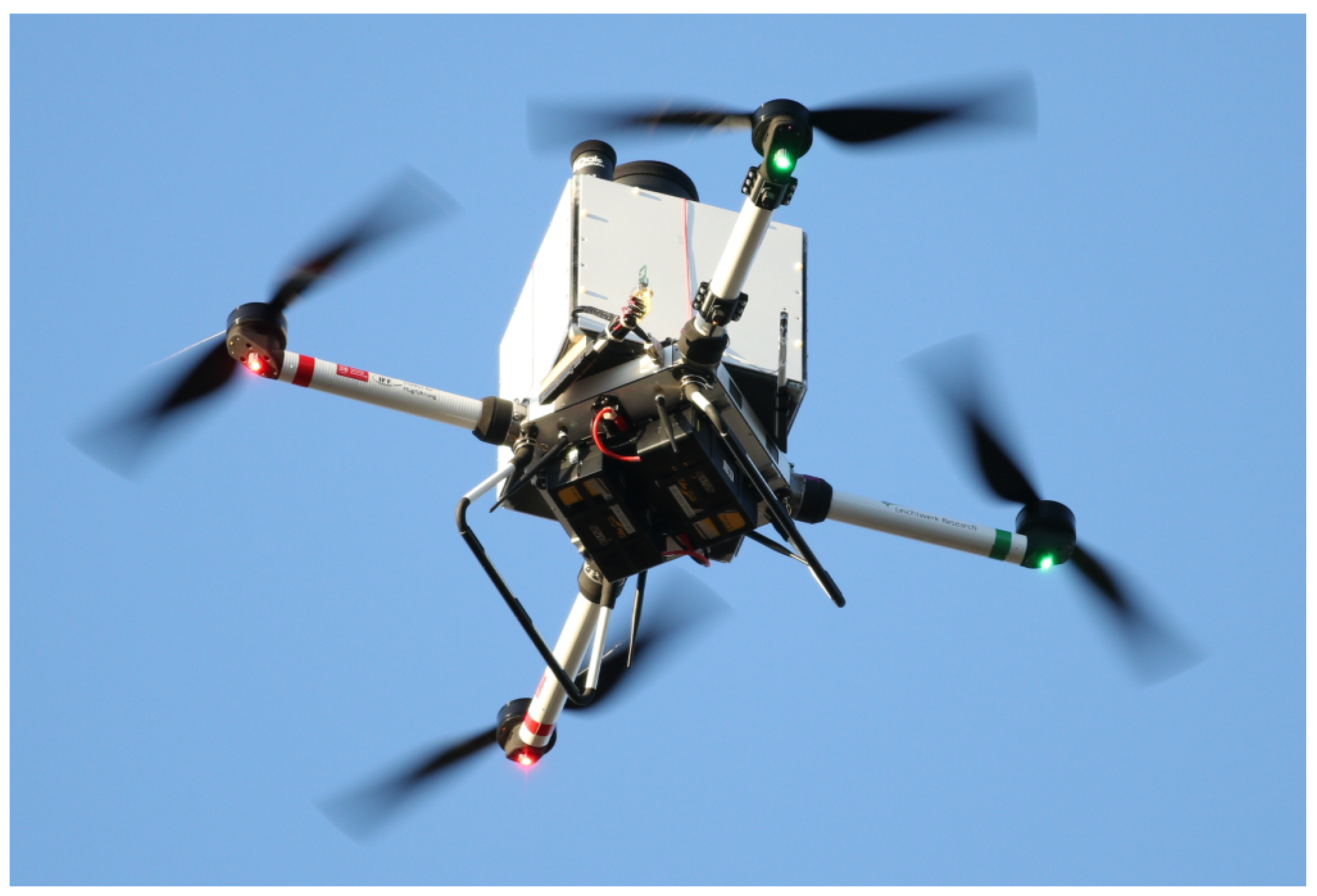
2.1. Quadcopter System

The quadcopter used for the study was designed for a maximum take-off weight of 25 kg, operations up to 1000 m altitude above ground to measure air quality parameters, and wind speed up to 35 km h${}^{-1}$ during take-off and landing, and up to 70 km h${}^{-1}$ in free flight [32,33]. The outer dimensions of the quadcopter are $1650\mathrm{mm}\times 1650\mathrm{mm}\times 300\mathrm{mm}$ with a cube-shaped payload housing of 370 mm edge length on top of a squared central base plate, and sensors and a safety parachute placed on top of it (Figure 1). Attached to the base plate are the four rotor arms with electric motors and propellers (Motor-P80III-KV100 and CF-PROP 30 × 10.5 with rotor radius $R=381\mathrm{mm}$ from Tiger Motor International Co.,Ltd, Nanchang, China). A rotor speed of about 2600 RPM (rounds per minute) is required for the operation of the quadcopter at 25 kg overall weight for hovering near ground, while the maximum rotor speed is 3747 RPM. Below the base plate there is a landing gear and a fixture for the propulsion system LiPo (Lithium Polymer) batteries (2 × 22 Ah, 6S1P) and the telemetry antennas for controlling the multicopter in manual mode, for commanding the autopilot (Pixhawk 2 from Hex Technology, Xiamen, Fujian, China) and for the real-time data transfer. Inside and above the payload cube, the measurement equipment for atmospheric research is installed. Depending on the battery system, a payload of up to 10.4 kg can be transported. A maximum only-vertical climb rate of 5 m s${}^{-1}$, an only-vertical descent rate of 2.5 m s${}^{-1}$, and a maximum horizontal speed of 20 m s${}^{-1}$ were demonstrated during the initial flight tests, and emergency descent maneuvers combining high vertical and horizontal airspeed were investigated. The applied batteries allow for a maximum safe flight duration of 15 min.

2.2. Flight Test Equipment

2.2.1. On-Board Instrumentation

The on-board measurement system mostly consisted of existing components from former projects. While this approach is very low in terms of costs, the sensors are not tailored to the specific needs of the envisaged experiments. Results and practical experience in measuring highly dynamic states were obtained in these previous projects, e.g., for qualifying the air sampling system on-board a quadcopter [1], but were not published due to their technical nature and the focus of the projects on scientific output. Pressure transducers, finewire temperature sensors, accelerometers, strain gauges, and sensors for determining the rotor state were placed at different positions on the multicopter, e.g., on the rotor arm or on separate mounts, that allowed sensor placement at different radial positions below one of the propellers, as shown in Figure 2.

Data Acquisition

The central element of the measurement system is a battery-powered SCADAS MOBILE system (SIEMENS AG/LMS) with 8 configurable analog-to-digital converters (A/D channels), LEA-6T GPS receiver (U Blox Holding AG, Thalwil, Switzerland) for time synchronization and positioning, and a data recorder. The system is located inside the payload cube and is reconfigured by a config file on the data storage SD card. The data recording rate can be set to up to $f_{\mathrm{rec}}=204.8$ kHz, but was chosen as $f_{\mathrm{rec}}=51.2$ kHz for all but one flight, see Table 1.

The available A/D channels limit the number of sensors that can be used simultaneously, so the investigations were carried out on one rotor arm as an example. A subset of the below presented sensors for rotor state, pressure, temperature, acceleration, and force was used in different combinations and at different radial distances from one of the propeller hubs, expressed as percentage of the propeller radius R, see Table 1. For a quick and simple implementation, additional batteries were used to power individual sensors, except the accelerometers that were fed by the data acquisition unit. Batteries provide a very low-noise supply voltage compared to regulated power supplies, but feature a slow voltage drift over time due to discharges, which can be easily filtered out, especially since we dealt with high frequency signals in this study. The usage of in-line voltage regulators would add some additional challenges—these devices emit electromagnetic radiation and cause interference, which requires suitable shielding. Damping the noise in the output voltage requires additional components that are usually temperature-dependent and affect the output voltage, which must be monitored to avoid signal misinterpretations. To overcome these supply issues, a radiometric analog-digital conversion has been used in previous work [34] but for the current study, the usage of batteries was considered the simplest overall approach.

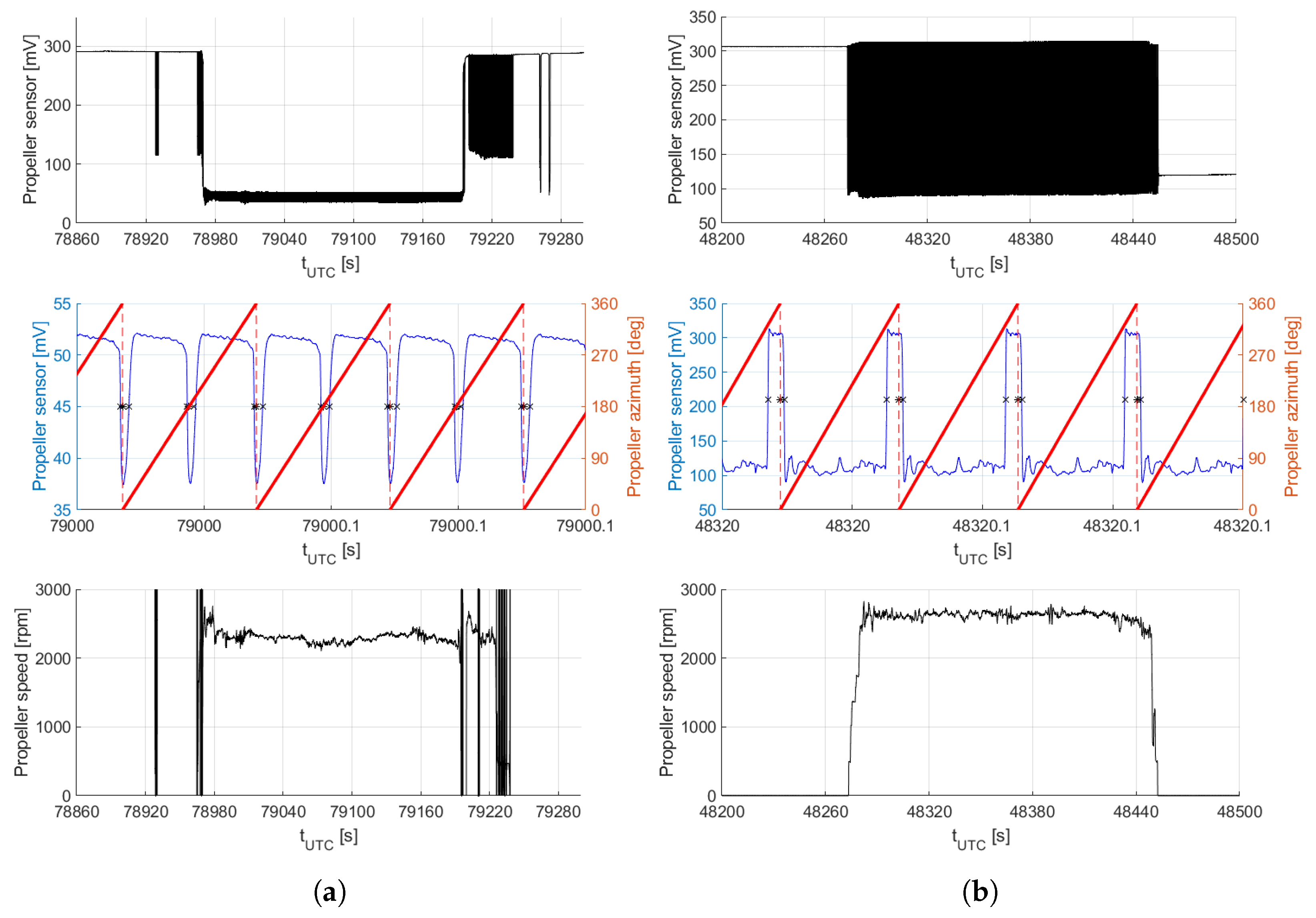
Rotor Speed of Rotation and Phase Sensing

For the present study, it was important to determine the azimuthal rotor position $\psi$ within each revolution (rotor phase), as the lift-generating rotor blades are the obvious main sources for disturbing the atmosphere and likely cause a significant portion of the vibrations on-board.

In a first try, an S9648-200SB photodetector amplifier (Hamamatsu Photonics K.K., Hamamatsu City, Japan) was mounted on top of the rotor arm. It was shielded with a small tube, faced upward to the sky, and thus was excited by the diffusely scattered sunlight (Figure 2, center picture). Each time a rotor blade passes the sensor, the measured signal drops. In practice, this approach is not robust, especially when the elevation of the sun is low: The sunlight can be reflected by the concave lower surface of the rotor blades and counteract the shading effect of the rotor blade, see Section 3.1. Rotor phase measurements are, in general, feasible with this approach, but the described disturbance effects necessitate improvements for practical application. The upgraded setup uses the same photo diode to detect a white tape added to the black, rotating motor housing. A plastic cover shields the photo diode from direct sunlight and a white LED placed inside the cover illuminates the motor housing constantly (Figure 2, bottom left picture). This setup delivers a clear signal proportional to the width of the white marking allowing a robust detection of each blade passage above a certain minimum speed of rotation (see Section 3.1). It is noted that this measurement concept is well suited for moderate and high rotational speeds, but becomes unreliable for rotor speeds close to zero, as the sensor can only detect the passage of the rotating white marking on the motor housing, as well as for changing sense of rotation, which the sensor cannot detect. This is critical, e.g., for harsh yaw maneuvers, where the rotor might even temporarily come to rest. A future refinement might be a set of white stripes with different widths at defined azimuthal positions for determining the direction of rotation and getting more accurate phase information during each revolution in case of accelerations.

Table 1. Overview of flight tests, highlighting flights used in this study in bold. The data analyzed in Section 3 is marked with green background. The checkmarks (✓) indicate usable raw data, crosses (X) indicate data that are not usable. [$\%R$] indicates the sensor position relative to the rotor radius. The data set is published in Pätzold et al. [35].

Flight	Date	Flight	Pressure		Temp.	3-Axis		Strain	BOS	Weight	Data	Rotor Speed	Temp.
No.	in 2021	Time	#1	#2	2×	Accel.		Gauges			Rate	Meas. Location	Housing
		[mm:ss]	[$\%\mathbf{R}$]	[$\%\mathbf{R}$]	[$\%\mathbf{R}$]	Outer	Inner	Vert.		[kg]	[kHz]
1	2 March	04:32	90.0	85.0	87.5	✓	–	–	–	21.8	51.2	Rotor	yes
2	2 March	11:25	87.5	82.5	87.5	–	X	–	X	21.8	51.2	Rotor	no
3	12 March	06:25	90.0	85.0	87.5	✓	–	–	–	24.9	51.2	Rotor	yes
4	22 March	08:37	87.5	82.5	X	–	X	–	–	24.9	51.2	✓	yes
5	22 March	04:56	92.5	87.5	X	–	X	–	–	24.9	51.2	✓	no
6	22 March	05:14	87.5	82.5	X	–	X	–	–	24.9	204.8	✓	no
7	23 March	07:58	–	87.5	–	✓	X	–	X	24.9	51.2	✓
8	23 March	02:52	90.0	85.0	X	✓	–	–	–	24.9	51.2	Motor	no
9	23 March	05:42	85.0	80.0	X	✓	–	–	–	24.9	51.2	Motor	no
10	23 March	01:14	95.0	90.0	X	✓	–	–	–	24.9	51.2	Motor	no
11	23 March	00:52	92.5	87.5	X	✓	–	–	–	24.9	51.2	Motor	no
12	23 March	00:55	87.5	82.5	X	✓	–	–	–	24.9	51.2	Motor	no
13	23 March	08:16	–	85.0	–	✓	X	–	✓	24.9	51.2	✓	-
14	23 March	06:45	–	90.0	–	✓	X	–	✓	24.9	51.2	✓	-
15	30 March	05:49	–	–	–	✓	✓	✓	–	24.9	51.2	Motor	-
16	30 March	05:20	–	–	–	✓	✓	X	–	24.9	51.2	✓	-

Table 1. Overview of flight tests, highlighting flights used in this study in bold. The data analyzed in Section 3 is marked with green background. The checkmarks (✓) indicate usable raw data, crosses (X) indicate data that are not usable. [$\%R$] indicates the sensor position relative to the rotor radius. The data set is published in Pätzold et al. [35].

Flight	Date	Flight	Pressure		Temp.	3-Axis		Strain	BOS	Weight	Data	Rotor Speed	Temp.
No.	in 2021	Time	#1	#2	2×	Accel.		Gauges			Rate	Meas. Location	Housing
		[mm:ss]	[$\%\mathbf{R}$]	[$\%\mathbf{R}$]	[$\%\mathbf{R}$]	Outer	Inner	Vert.		[kg]	[kHz]
1	2 March	04:32	90.0	85.0	87.5	✓	–	–	–	21.8	51.2	Rotor	yes
2	2 March	11:25	87.5	82.5	87.5	–	X	–	X	21.8	51.2	Rotor	no
3	12 March	06:25	90.0	85.0	87.5	✓	–	–	–	24.9	51.2	Rotor	yes
4	22 March	08:37	87.5	82.5	X	–	X	–	–	24.9	51.2	✓	yes
5	22 March	04:56	92.5	87.5	X	–	X	–	–	24.9	51.2	✓	no
6	22 March	05:14	87.5	82.5	X	–	X	–	–	24.9	204.8	✓	no
7	23 March	07:58	–	87.5	–	✓	X	–	X	24.9	51.2	✓
8	23 March	02:52	90.0	85.0	X	✓	–	–	–	24.9	51.2	Motor	no
9	23 March	05:42	85.0	80.0	X	✓	–	–	–	24.9	51.2	Motor	no
10	23 March	01:14	95.0	90.0	X	✓	–	–	–	24.9	51.2	Motor	no
11	23 March	00:52	92.5	87.5	X	✓	–	–	–	24.9	51.2	Motor	no
12	23 March	00:55	87.5	82.5	X	✓	–	–	–	24.9	51.2	Motor	no
13	23 March	08:16	–	85.0	–	✓	X	–	✓	24.9	51.2	✓	-
14	23 March	06:45	–	90.0	–	✓	X	–	✓	24.9	51.2	✓	-
15	30 March	05:49	–	–	–	✓	✓	✓	–	24.9	51.2	Motor	-
16	30 March	05:20	–	–	–	✓	✓	X	–	24.9	51.2	✓	-

The uncertainty of the rotor phase $\psi$ during the later analyzed hover flight sections is estimated as ≤2${}^{\circ }$. A value of $\psi =0^{\circ }$ is defined as the passage of the quarter-chord line of one of the two blades directly above the rotor arm, as highlighted in the bottom left of Figure 2. The same rotor blade passes the rotor arm again at $\psi ={360}^{\circ }$, but the two-bladed rotor system was highly symmetrical, enabling a comparison of each separate blade passage with a repetition after $\psi ={180}^{\circ }$.

Pressure Sensors

Two XT-190M-1BARA pressure transducers (Kulite Semiconductor Products, Inc., Leonia, NJ, USA) [36] were mounted vertically and facing upwards on an adjustable support arm, resulting in a sensor inlet position 55 mm below the rotor blades quarter-chord line plane. The support arm was located at a rotor phase angle of $\psi =18.2^{\circ }$ and oriented along the radial direction. The two sensors featured a fixed radial distance of $5\%R$ and were set at different radial positions between $80\%R$ and $95\%R$ between flights to cover the outer part of the rotor downwash (Figure 2, top right picture, and Table 1). As the recorded measurement signals of the sensors also exhibited the voltage drift described in the Data acquisition section above, they were corrected using the ambient static pressure measurements recorded with rotors turned off on the ground directly before and after each test flight. These reference measurements were also used to determine the calibration factor between the recorded voltages and externally measured ambient pressure. As the pressure fluctuations are of interest here, the signals were bandpass-filtered using first order Butterworth phase-free filtering with cutoff frequencies at 1 Hz and 5120 Hz ($f_{\mathrm{rec}}/10$) to obtain proper amplitude information.

Temperature Sensors

The temperature measurements were carried out using a two-channel resistive temperature sensor that was developed and characterized at the Institute of Flight Guidance at Technische Universität Braunschweig [34]. The sensor consists of a thin rectangular support frame with a rectangular window of $20\mathrm{mm}\times 10\mathrm{mm}$ dimensions in which multiple 12.5 $\mathsf{\mu }$m thick platinum wires are placed. Finewire 1 consists of two parallel wires of 20 mm length positioned parallel to the main flow direction, and Finewire 2 consists of four parallel wires of 10 mm length oriented normal to the main flow direction. The sensor was vertically positioned below the rotor on a second adjustable support arm on the opposite side of the rotor arm at a fixed azimuthal position of $\psi =-19.4^{\circ }$, a fixed radial distance to the rotor axis of $87.5\%R$, and an approximate sensor center position at 52 mm below the rotor plane (Figure 2, top left picture). The sensor was originally designed for fixed-wing drone air temperature measurements that were fast enough to determine meteorological fluxes while being resilient to particles that can destroy fine wires. This robust design, however, limits the dynamic range of the sensor (see Section 2.3.1). To shield the sensor from sun and airframe heat radiation and to provide stagnation point conditions (total air temperature), usually a cylindrical housing is fitted around the sensor [34]. For some flights, this housing was used, see Table 1, but it turned out that the finewires are robust enough to be operated without this housing.

Accelerometers

Two 356A16 triaxial accelerometers (PCB Piezotronics, Inc, Depew, NY, USA; rated measurement range 500 m s${}^{-2}$ at 0.5 to 5000 Hz; 10 mV per 1 m s${}^{-2}$) were mounted at the bottom side of the rotor arm at radial distances of 60 mm ($15.7\%R$) and 285 mm ($74.8\%R$) from the rotor axis using 3D-printed clamps (Figure 2, bottom right picture, x-axis parallel to rotor arm tube, y-axis perpendicular to x-axis in the rotor plane and z-axis perpendicular to x-y-plane). The chosen locations qualitatively represent the vibrations at the inner and outer end of the rotor arm.

Strain Gauges for Rotor Force Measurements

Four standard 120 $\mathsf{\Omega }$ strain gauges were interconnected to a full Wheatstone bridge, which is an electrical circuit that transforms the change in electrical resistance occurring on the strain gauge sensors into a measurable voltage signal., with two strain gauges at the top and two at the bottom of the rotor arm tube root for the vertical force measurements (Figure 2, center right picture). For feeding, amplifying, and filtering this resistor network, a BA660 module (Vishay Intertechnology, Inc, Malvern, PA, USA) was used, which was hardware-configured with a 2nd order low-pass Bessel filter with −3 dB at 250 Hz. A second set of strain gauges was applied in the horizontal plane but did not deliver proper data due to a wiring issue.

The signal of the strain gauges reading was converted to a vertical force in two ways: first, the quadcopter was flipped before and after the flight to use the known weight of the rotor arm as calibrated masses to obtain a calibration function; second, the mean force measured in-flight was assumed to be a quarter of the force needed to compensate the known quadcopter weight. The resulting force difference is below 5% or 5 N and assumed to be sufficiently small for this investigation. It must be kept in mind that the determined force will be close but not equal to the thrust of the propeller, because it is influenced by the propeller down-wash acting on the rotor arm in a small manner.

2.2.2. External Measurement Systems

As previously mentioned, the main source of aerodynamic fluctuations on the quadcopter is the rotors and their wake. The dominant flow feature in the rotor wakes is the vortex created at the tip of each blade. The relative strength and position of these blade tip vortices are critical in understanding their effects on the local fluctuations in the pressure and temperature field. However, reliable predictions of the trajectories, strength, and decay of these vortices is still challenging, and in-flight measurement data for validation is sparse. For this reason, vortex visualization based on the Background-Oriented Schlieren (BOS) method was carried out during some of the flight tests. The core of a sufficiently strong vortex features a region of reduced air density $\rho$.

The BOS method can then be utilized to visualize vortices by tracking changes in the refractive index n of air caused by these spatial density gradients. The density and refractive index are related by the Gladstone–Dale equation

$$n-1=K·\rho ,$$

(1)

with the Gladstone–Dale constant K. For the standard BOS method, a single camera focuses on a background pattern situated behind the density distortion [37], as shown in Figure 3a. The change in refractive index n causes an angular deflection ${\epsilon }_y$ along y (and ${\epsilon }_x$ along x) of incident light rays [38]:

$$tan\left({\epsilon }_y\right)={\int }_0^{Z_{\mathrm{B}}}\frac{1}{n}\frac{\partial n}{\partial y}dz.$$

(2)

With this method, an integral measure of density gradients along the line-of-sight z is obtained, spanning the distance from the observer to the background at $z=Z_{\mathrm{B}}$. The small deflection angles ${\epsilon }_x$ and ${\epsilon }_y$ produce an apparent displacement $(u,v)$ of the recorded background pattern in the x and y direction:

$$(u,v)=Z_{\mathrm{D}}M{\epsilon }_{x,y},$$

(3)

where $M=Z_{\mathrm{i}}/Z_{\mathrm{B}}$ is the magnification factor of the background, $Z_{\mathrm{i}}$ the focal length of the camera objective, and $Z_{\mathrm{D}}$ the distance between the density distortion and the background. This apparent displacement field $(u,v)$ is obtained, e.g., by performing a sequential cross-correlation evaluation between corresponding sections of the undistorted background (reference image) and measurement image including the density distortion in the object plane. The obtained apparent displacement field is consequently proportional to the density gradients spatially integrated along the line-of-sight.

A variation of this standard BOS method, the reference-free BOS approach, is shown in Figure 3b. This method has been shown in previous studies to be highly suitable for the visualization of helicopter blade tip vortices under free maneuvering flight conditions [39,40]. The method was also applied here for rotor blade tip vortex visualization on the free-flying quadcopter. This variant method uses the fact that significant distortions of the density field—and therefore the refractive index field—only occur in spatially limited wake regions of typical rotary wing aircraft, and move relative to the background with time. It then becomes possible to evaluate two temporally separated measurement images of the rotorcraft (at points in time $t_1$ and $t_2$ in Figure 3b) with the same background structure against each other, so the undisturbed parts of one of the images serve as a reference for the other image and vice versa. For both the reference-free and standard BOS method, either artificial dot patterns or naturally occurring structures with a sufficiently high contrast and spatial frequency can be used [41].

A reference-free BOS setup with an airborne camera was realized in the present flight tests to evaluate the visualization capability for hover flight outside of the ground effect. A second drone (Matrice 600 Pro, SZ DJI Technology Co., Ltd, Shenzhen, China) flew at a height of 100 m and above the quadcopter, which was operated at a height of 50 m above ground. The camera drone was equipped with an iXM-100 camera (Phase One, Copenhagen, Denmark) with a resolution of 100 megapixels and a 150 mm lens (Phase One). The setup allowed remote-controlled acquisition of pictures capturing coarse structures on the naturally illuminated tarmac with the quadcopter flying in the foreground of the field of view.

After the test runs, matching pairs of images taken at very similar observation positions were selected and evaluated against each other. These image pairs were mapped onto each other using a Matlab routine and were processed in the PIV (Particle Image Velocimetry) software Davis 8.4 (Lavision GmbH, Göttingen, Germany) using a multi-grid cross-correlation scheme with a final interrogation window size of $16\mathrm{pixels}\times 16\mathrm{pixels}$ and $75\%$ window overlap. The resulting displacement fields $(u,v)$ were post-processed with an outlier filter that removed spurious vectors that deviated by more than two standard deviations from neighboring vectors and replaced them by interpolated vectors. The threshold was adjusted to remove displacements with a low correlation coefficient $\le 0.1$, indicative of insufficiently high background contrast for valid cross-correlation results. The corresponding divergence field of the displacements was derived as:

$$\mathrm{div}=\frac{\partial u}{\partial x}+\frac{\partial v}{\partial y}.$$

(4)

This operator is used for visualization of blade tip vortices and other small-scale structures in the rotor wake, as it is less susceptible to large-scale displacement patterns [39].

Despite the large overall field of view of the in-flight setup, each rotor of the quadcopter is only resolved with about $1800\mathrm{pixels}\times 1000$ pixels in the acquired images that will be discussed in Section 3.2.3. Combined with a vortex core diameter of ≤$2.5\%R$ that was experimentally determined with PIV in laboratory tests of one of the current multicopter propellers, the vortices are only resolved with about 12–20 pixels each, compared to an interrogation window size of $16\mathrm{pixels}\times 16\mathrm{pixels}$ for the data processing. Together with the relatively coarse and low-contrast background structures available at the flight test location, this illustrates that further vast improvements are possible for the in-flight application of this visualization method.

2.3. Laboratory and Ground Tests

2.3.1. Laboratory Tests of On-Board Measurement Equipment

Besides functionality checks and static calibrations of the temperature sensor, pressure sensors and force determination, the noise floor level of the sensors was measured to ensure that in-flight measured signals are sufficiently above the inherent noise level of each sensor. Additionally, the temperature and pressure sensors were excited using a hot-air gun (HG2310 LCD, Steinel Solutions AG, Einsiedeln, Switzerland) operated with and without heating at maximum fan speed. It cannot be expected that the obviously turbulent air flow follows idealized noise laws. Looking at the fan diameter, speed of rotation, nozzle geometry and audible noise, a turbulent flow at energy levels well above atmospheric turbulence can be assumed without knowing the respective excitation spectra. Based on this excitation, a rough impression about the spectral transfer behavior of these sensors can be obtained.

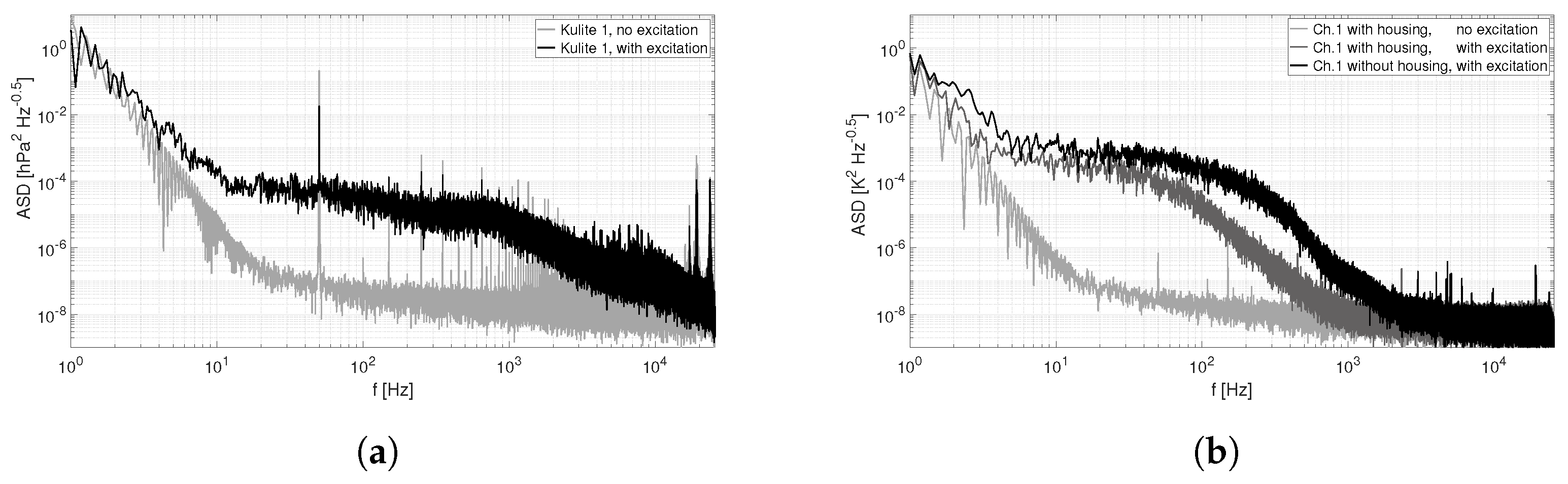
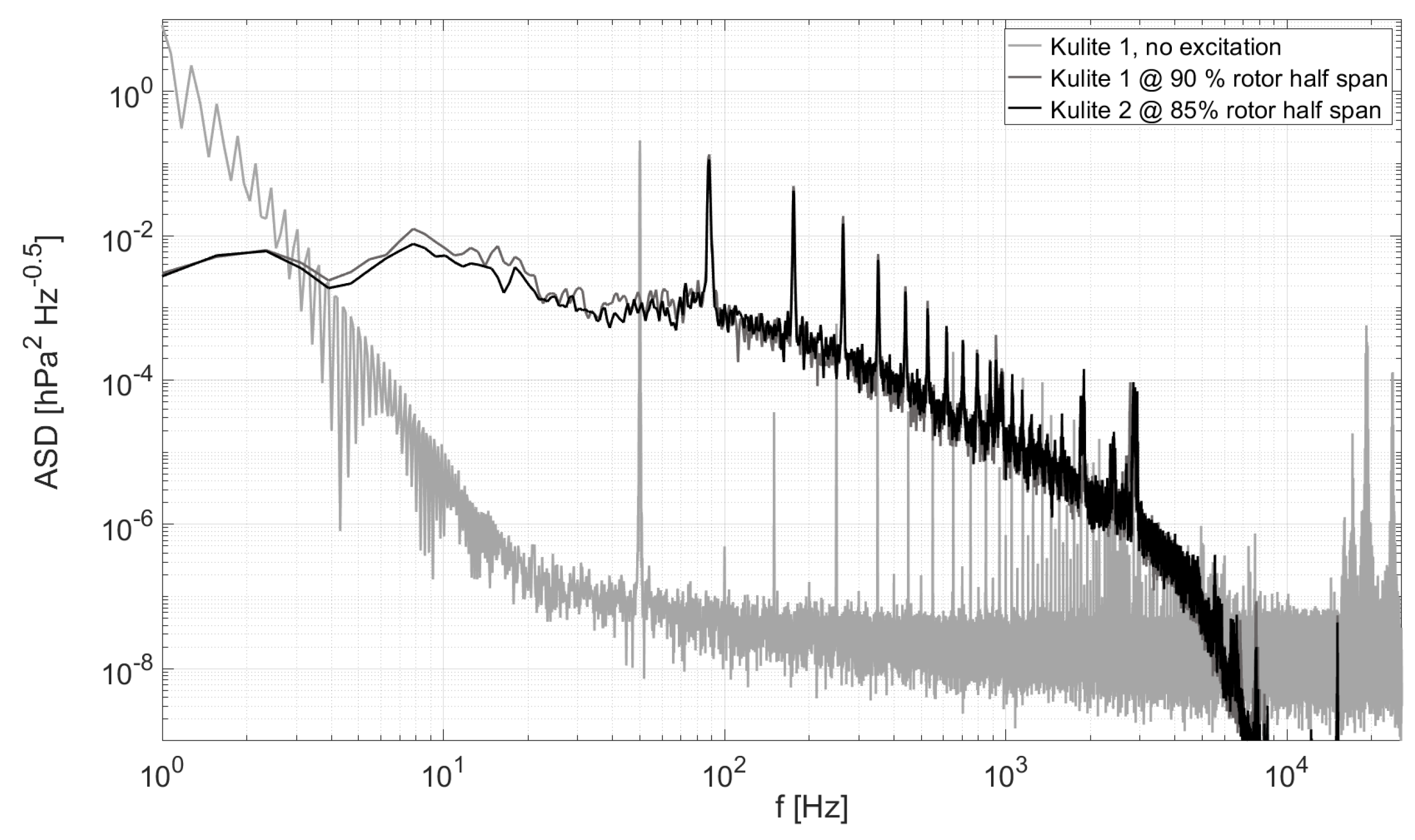
Spectra of Kulite Pressure Sensors

Both Kulite pressure sensors were excited in the laboratory at the same time with different angles of incident and distances to the heat gun’s nozzle and analyzed in the spectral domain. Both sensors showed roughly the same amplitude spectral density (ASD) for all setups. Figure 4a shows unexcited spectra of Sensor 1 as ASD, as well as spectra with hot-air gun excitation normal to the sensor’s inlet area. The noise level without excitation drops with rising frequency until it reaches a near-constant level. The excitation adds pressure fluctuations within the whole frequency range to the spectrum. Below 10 Hz the high pass characteristics of the sensor feeding can be seen and the decay above 700 Hz might indicate the upper excitation frequency limit.

The significant peaks at 50 Hz and the higher harmonics result from the electromagnetic coupling of the 230 VAC laboratory power grid into the measurement system. This is quite common and can be solved with high technical effort like electromagnetic shielding/decoupling or by suppressing these known frequencies numerically. This electromagnetic receptivity must be kept in mind for the application on the quadcopter with its electric propulsion.

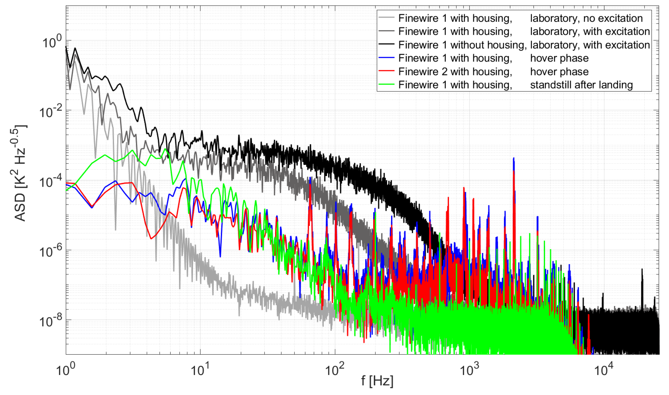
Spectra of Finewire Temperature Sensors

The finewire temperature sensors were examined in the same way, with similar results (Figure 4b). Both finewires result in nearly the same spectral results, despite the differences in the sensor geometry. Spectra without excitation show a clear receptivity to the 50 Hz house power grid. Replacing both finewire by standard resistors does not influence the noise floor level, thus the finewire parts are not the locations where this electromagnetic coupling occurs. The cylindrical housing around the sensor described in Section 2.2.1 has an amplitude reducing effect on the resulting spectrum of the excited sensors. This is caused by the flow braking design of the housing, resulting in stagnation point conditions inside the housing. The steeper slope above 40 Hz in the excited and housed sensor spectrum and above appr. 200 Hz in the excited and non-housed sensor spectrum might indicate the lowpass filtering effect due to the sensors’ thermal capacity. The presented spectra do not constitute a proper system characterization, as the used excitation is not characterized itself.

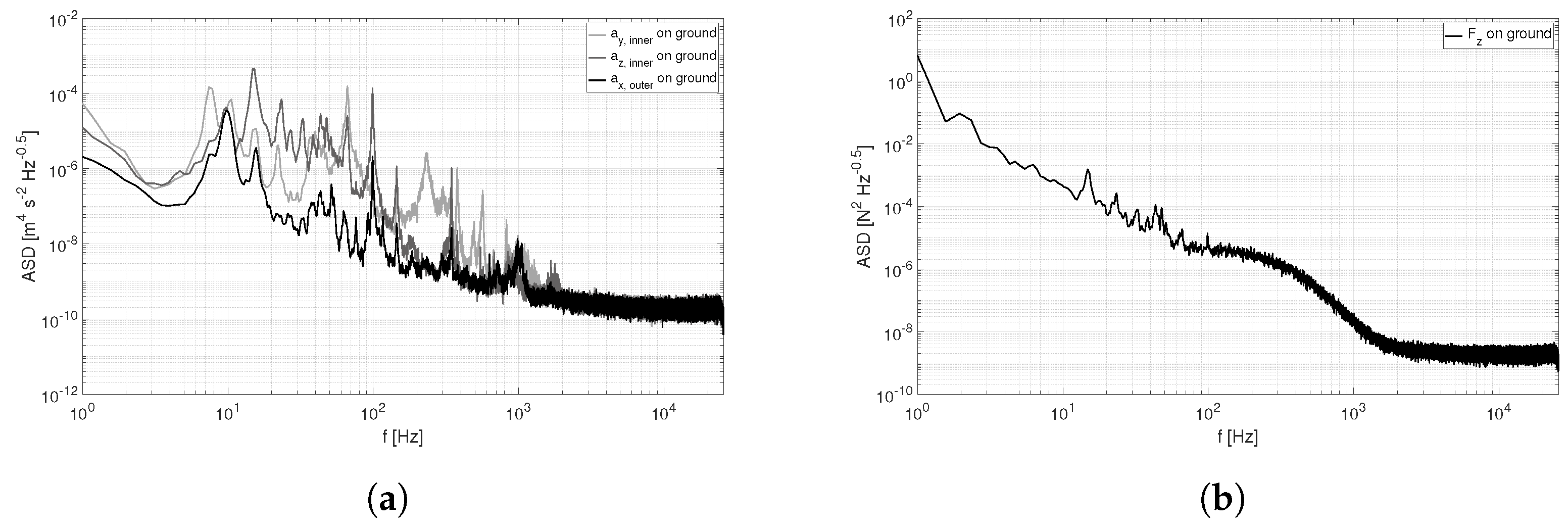
Spectra of Accelerometers and Force Measurements

The spectra of the accelerometers and the strain gauges used for force measurements are shown in Figure 5a,b. They were obtained from a 30 s section before Flight 15 while the quadcopter was standing on the ground. Therefore, they are not affected by interference with the a 230 VAC power grid, but show the elastic reaction of the copter to turbulent wind on the ground. The interpretation of the spectra obtained shall be limited here to the conservative classification of the order of magnitude of the noise of the sensors without excitation.

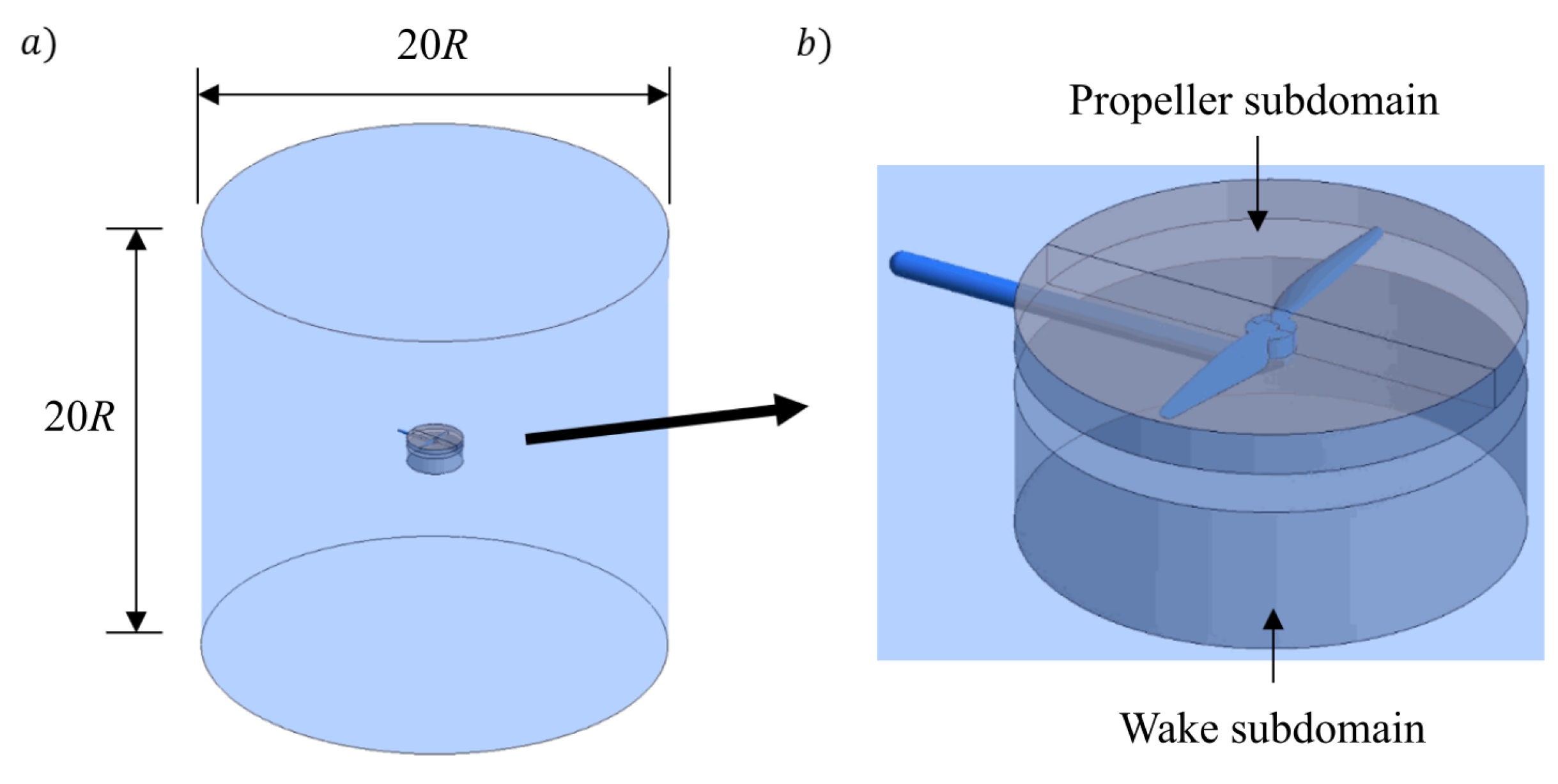
2.3.2. Laboratory Setup for Hover Tests with Isolated Rotor

A hover test was conducted with an isolated two-bladed propeller of the quadcopter system to generate aerodynamic reference data for the flight tests. The rotor was powered by its regular motor with an electronic speed controller, and controlled with Labview software (National Instruments Corporation, Austin, TX, USA) through an Arduino Uno computer board (Arduino, New York, NY, USA). The motor was mounted on a rotor arm of $670\mathrm{mm}$ length and $44\mathrm{mm}$ outer diameter, as shown in Figure 6, in a setup comparable to the full quadcopter. The rotor setup was placed on a rigid aluminum structure and operated at a height of $z=2.4\mathrm{m}$ or $z=6.3R$ above the ground, effectively out of ground effect according to [42]. The clearance of the rotor in all other directions was higher, between $10R$ and $20R$. The rotor stand included a sting balance for measuring rotor thrust, torque, and vibratory levels. For each test condition, 7000 data points were acquired at a measurement frequency of $1200\mathrm{Hz}$ (263 rotor revolutions) and averaged to obtain mean loads. The test stand further contained a photoelectric sensor for quantifying the rotational speed and additional sensors for measuring the electric power consumption, monitoring the motor temperature, and acquiring the ambient air conditions. The propeller was operated at its nominal thrust level for hover of $T_0=62\mathrm{N}$, specified based on one quarter of the nominal weight force of the quadcopter. This thrust was reached for a nominal rotational speed of $\mathsf{\Omega }=283.58\mathrm{rad}{\mathrm{s}}^{-1}$ ($2708\mathrm{RPM}$). Similar rotational speeds between 2500 RPM and 2700 RPM were obtained during the hover phase of the flight tests.

The wake of the rotor was characterized based on particle image velocimetry (PIV) and BOS measurements. Representative results of the performance and PIV measurements will be reported in a different publication, while the current work only involves the BOS results.

Contrary to the previously described reference-free BOS system applied during the flight tests, a classical BOS approach was chosen during the laboratory hover tests. The laboratory BOS setup employed a PCO.4000 camera (Excelitas PCO GmbH, Kelheim, Germany) with a lens featuring an effective focal length of $412\mathrm{mm}$. The camera was focused on a retro-reflective screen of $0.7\mathrm{m}\times 1.0\mathrm{m}$ dimensions that was printed with a random dot pattern of $0.5\mathrm{mm}$ dot diameter and placed at a distance of $Z_{\mathrm{B}}=10.4\mathrm{m}$ from the camera. The pattern was illuminated by a constant light source placed directly behind the camera. The rotor was located at a distance of $Z_{\mathrm{D}}=5.0\mathrm{m}$ in front of the background and the BOS system covered a field of view of about $1.3R$ in the horizontal and $0.85R$ in the vertical direction, centered on the rotor arm. Prior to each test run, an undisturbed reference image was acquired and evaluated against measurement images recorded during rotor operation. These image pairs were mapped onto one other and evaluated in the same way as the mapped image pairs from the flight tests (Section 2.2.2), including the same processing and post-processing settings. Results of the BOS measurements are shown in Section 3.2.3.

2.4. Numerical Setup for Simulations of Isolated Rotor

A reference data set was obtained using computational fluid dynamics (CFD) simulations. The flow around an isolated propeller under hover conditions was investigated with Fluent 2020 R2 (Ansys, Inc., Canonsburg, PA, USA). A geometry similar to the hover test setup was modelled, consisting of a full rotor, motor, and test stand arm, as shown in Figure 7a. The computational domain is split into a rotating flat cylinder around the rotor blades, embedded into the center of a stationary outer cylinder, as depicted in Figure 7b. The outer cylinder has a diameter and height of 20 rotor radii R, respectively, while the inner domain has a diameter of $2.36R$ and a height of $1.14R$. The two subdomains are connected via interface conditions to provide undisturbed flow between them. Model surfaces are treated as adiabatic walls with no-slip conditions to properly consider viscous effects, but ignore heat transfer to and from the solids, which was deemed mostly negligible for the current case. Future studies will take into account the heat transfer at the motor surfaces. The outer surface of the outer subdomain is set as a far field boundary with pressure $p_{\infty }$ and temperature $T_{\infty }$, corresponding to the experimental test conditions. The inner subdomain was resolved with a relatively fine mesh of homogeneous cells and local refinement near the walls through inflation layers, while the outer subdomain featured an increasing mesh size away from its interface with the inner subdomain.

A mesh independence study was carried out, resulting in a final mesh with about $9.5$ million elements. Adaptive mesh refinement was implemented to increase the mesh resolution in the vicinity of the rotor’s tip vortices based on the Q criterion, which is a field operator commonly applied for vortex detection based on the second invariant of the velocity gradient tensor [43]. This measure guaranteed proper resolution of the vortex topology, effectively preventing unrealistically high vortex diffusion in the rotor wake. The $k-ϵ$ realizable turbulence model [44] was employed, which has been shown to properly capture wake flows of rotating airfoils [45,46]. The boundary layer on the propeller blade surface was resolved with $y^{+}\approx 30$. Enhanced wall treatment was used for the boundary layers, which were modelled as fully turbulent. This assumption is anticipated to have a slight impact on the calculated rotor torque, but not on rotor thrust and the wake topology, which are of primary interest here.

Time-resolved simulations were conducted considering a relative rotational motion of the inner subdomain around the rotor axis. The simulations considered the fluid as a compressible ideal gas and solved the compressible Reynolds-Averaged Navier–Stokes (RANS) equations with the continuity, energy, and turbulence equations. These are the governing equations for the flow-physical problem under investigation and the basis for most numerical flow simulations. Compressibility has to be considered here, as typical blade tip Mach numbers are on the order of $M_{\mathrm{tip}}=0.3$, with local Mach numbers above this value leading to density changes on the order of ≥5%. The energy equation included heating due to viscous work. The fully-coupled pressure correction approach was used, as well as second order schemes for all convective terms.

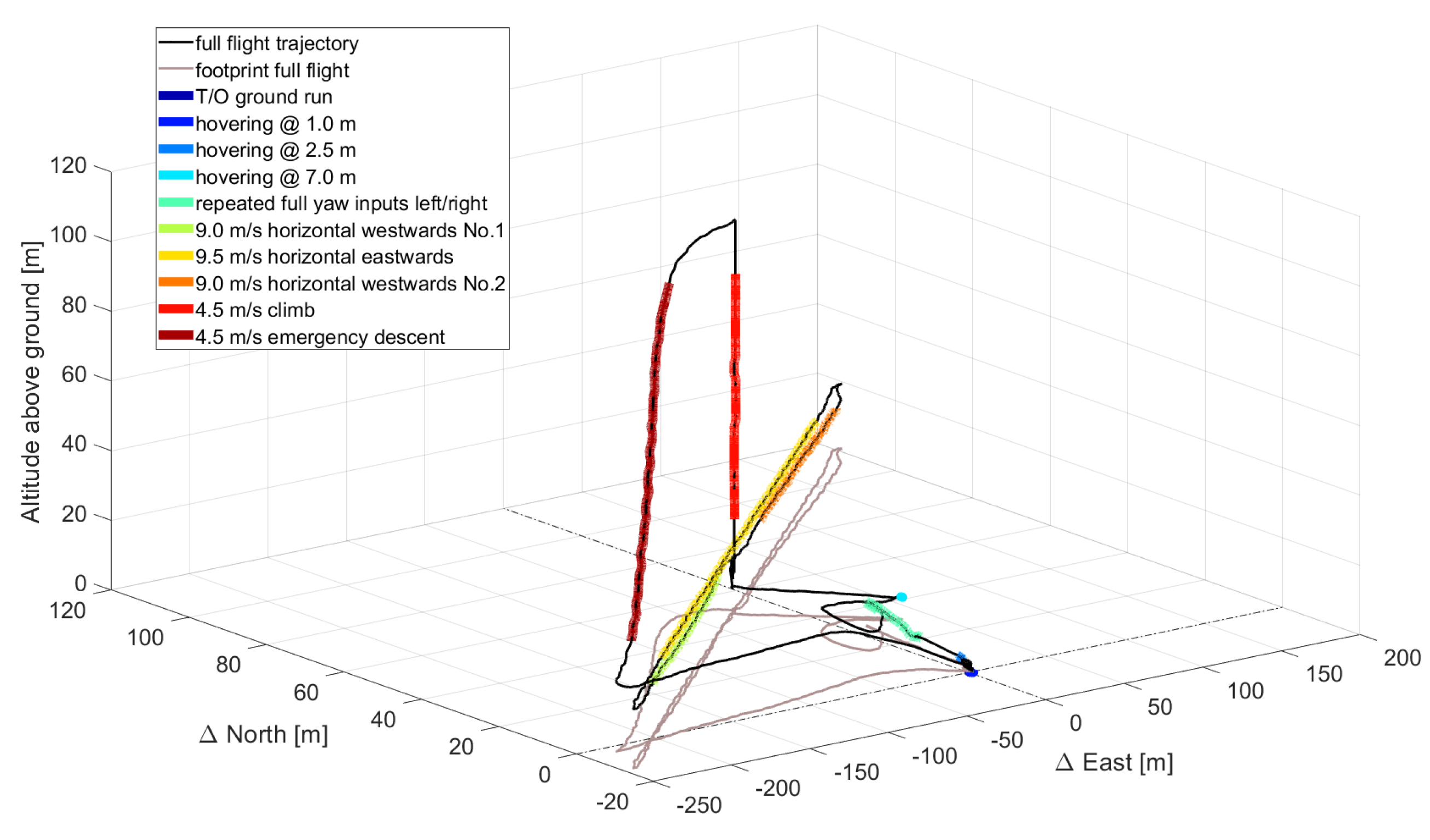
2.5. Flight Test Overview

The test flights were primarily conducted to test and investigate the basic handling characteristics and performance of the newly developed quadcopter system. Several flights took place between 2 March and 30 March 2021 at the former airfield Peine-Eddesse, Germany. Beginning with hover flights at low altitude, the flight envelope was expanded by flying and assessing a set of maneuvers, each increasing one of the flight parameter, e.g., the climb rate or the horizontal speed. An example test run is shown in Figure 8, where different flight phases are marked in the flight trajectory of Flight 15.

A summary of the test flights is given in Table 1. A total of 16 flights were conducted with the described measurement system, with an overall flight time of approximately 87 min. For all flights the weather was windy with moderate turbulence and wind speed of 4–8 m s${}^{-1}$ at 2 m above ground, and clear to overcast sky.

The flights were manually divided into typical flight phases. Although several analyses and comparisons were carried out, this paper focuses on the hover flight phases, as the results here are much more reproducible and clearer than in all other flight phases.

3. Results and Discussion

The present study is based on a subset of the available flight data, as detailed in Table 1. The full data sets are published in Pätzold et al. [35]. Furthermore, only hover flight segments that exhibited stationary operating conditions over a period of time of at least 4 s were chosen for the following results, as observing dynamic processes in a disturbed atmosphere requires a high rate of repetitions or increased number of sensors to ensure representative results.

3.1. Measurement of Rotor Speed and Phase

Figure 9 shows example results of rotor speed and phase measurements for Flight 1 and Flight 8. The selected flights both feature take-off, quasi-steady hover out-of-ground effect and landing, but with two differently realized setups for the rotor speed measurements. The weight of the quadcopter changed between the two setups, leading to noticeably different rotor speeds. For the first setup, the peak-to-peak variations of the raw signal are relatively low and the signal amplitude is not stable, as it quite obviously depends on the cloud coverage and the sensor’s relative position to the sun. Each rotor blade passage is detectable in the signal, resulting in two phase measurements per rotor revolution. On the other hand, the second setup with an active and shielded light source yields much higher signal amplitudes with steep and robustly detectable edges. Despite the reduction to only one phase measurement per revolution at the time of these measurements, this increased signal strength results in much more reliable measurements. Using the first time derivative of the sensor’s voltage signal, the resulting minima and maxima are used to detect the edges of the signal and thus the points of zero rotor phase, where the assumed quarter chord line passes the rotor center line of the rotor arm. This time series of zero phase crossings is spline interpolated to smooth the signal, and the rotor speed is calculated based on time increments between consecutive zero phase crossings.

As can be seen from the strong fluctuations in the detected rotor speed at the beginning and end of the analyzed flight test signal, the first setup requires a certain minimum speed of rotation to produce meaningful results. In contrast, the second setup provides reliable rotor speed results also at low rotor speeds, and therefore is more suitable for test cases with varying rotor speed. Using additional markings on the motor housing could gradually improve the measurement resolution of the second setup and further improve the determination of fluctuating rotor speed, especially for maneuvers with low speed of rotation.

3.2. Aerodynamic Results

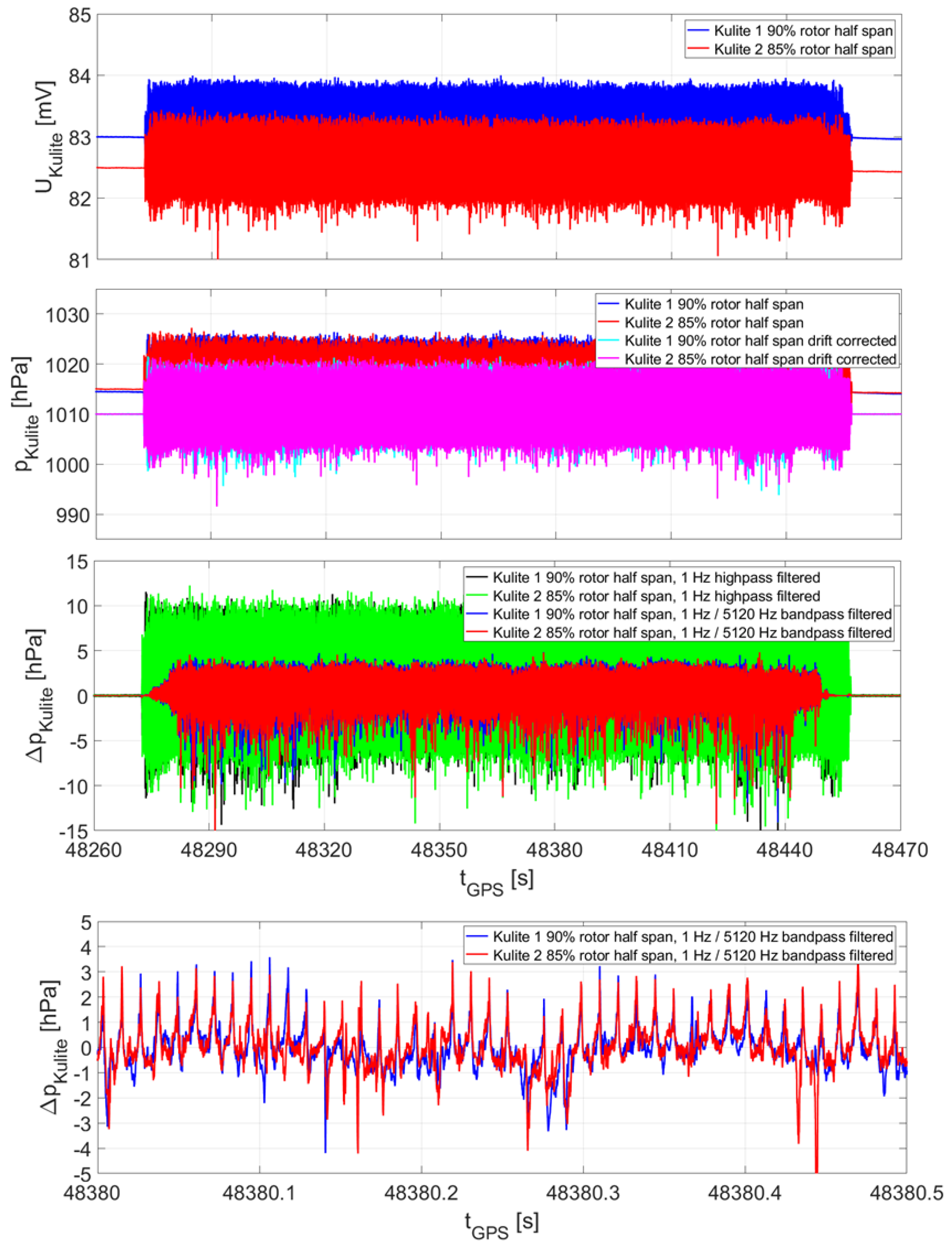
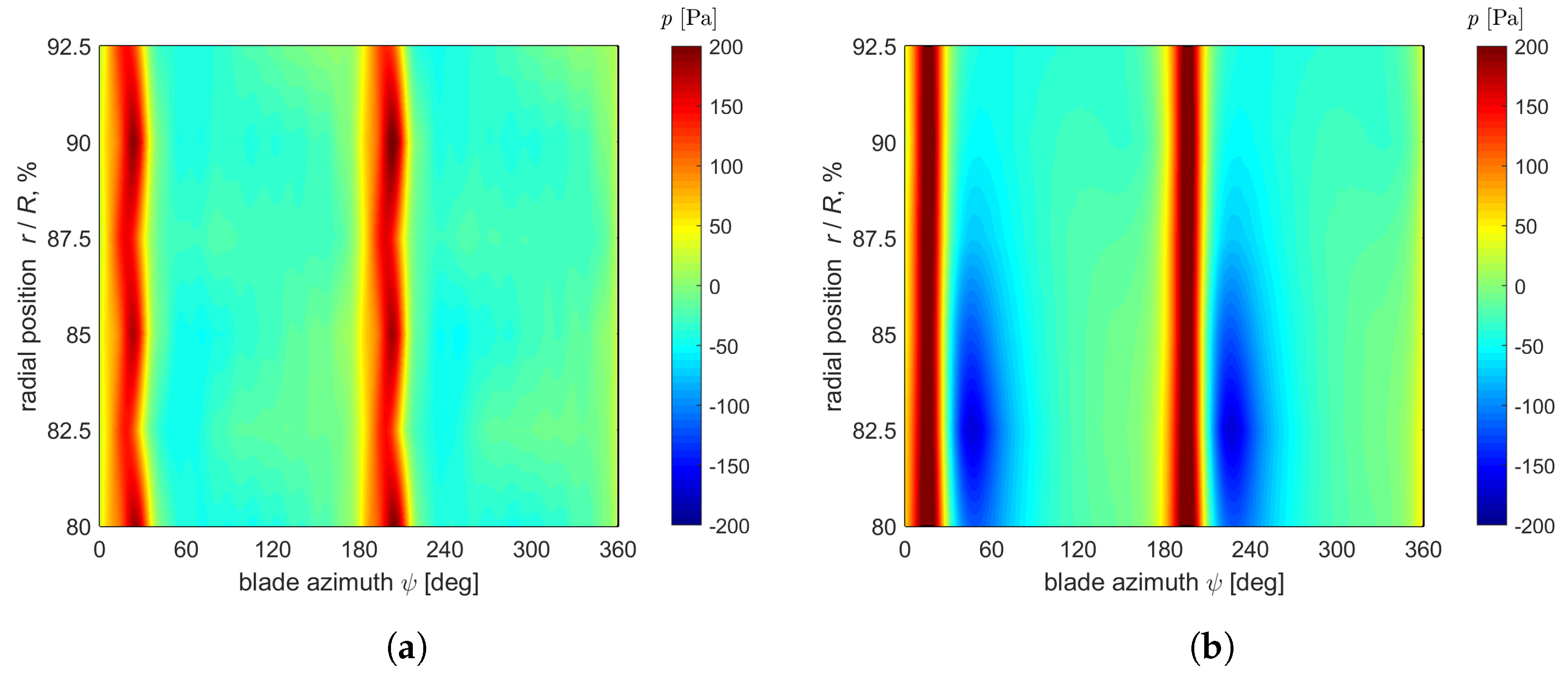
3.2.1. Pressure Fluctuations Induced by Rotors

For Flight 8, the raw signal of the pressure sensors and some processing steps are shown in Figure 10. The top panel shows the recorded voltage signal of the two sensors over a full flight cycle. The second panel depicts the corresponding calibrated absolute pressure signals, before and after correcting the sensor drift caused by the power supply voltage. Finally, the pressure fluctuations relative to static ambient pressure given in the two bottom panels were derived using a 1 Hz highpass- and a 1 Hz to $f_{\mathrm{rec}}/10$ bandpass-filtering. A significantly non-symmetric amplitude difference can be noticed between both results, but is hard to explain without in-depth numerical analyses which include the sensor itself. Analyzing the pressure fluctuations in the bottom panel of Figure 10, it can be seen that the wake of each propeller blade causes a characteristic pressure fluctuation. Although these fluctuations are quite similar, their exact shape changes rapidly between different rotor blade passes and over a few rotor revolutions. These changes at different time scales occur even for stable hover. Considerations to explain this behavior again lead to the need for detailed numerical modelling of the structure and fluid mechanics, as well as a significantly extended measurement technique to determine the characteristic properties of each rotor in a time-resolved manner. The holes of the pressure sensors faced upwards to primarily measure fluctuations in the downward flow speed. As the angle of incident at the plane of the holes was not observed, larger flow angles in the order of magnitude exceeding ${10}^{\circ }$ may result in a distorted pressure signal in the order of magnitude of 10% [47]. Thus, including the sensor and its aerodynamic design into future numerical simulations is essential.

An 8 s section of the hover flight partly shown in the bottom panel of Figure 10 was analyzed for both pressure sensors and is shown with the spectrum of an unexcited sensor in Figure 11. With the in-flight pressure spectral energy up to five orders of magnitude above the laboratory test spectrum, the signal-to-noise ratio is sufficient to be interpreted without taking noise into account. In the in-flight data, the first spike at about 90 Hz corresponds to the primary wake of each blade and therefore occurs at twice the speed of rotation. The occurrence of higher harmonics of this primary excitation is typical for rotor applications and may indicate a complex repeating flow pattern in the wake. At a frequency of around 950 Hz a broader spike can be seen. This frequency corresponds to 21/rev, matching the number of 21 magnet segments of the electric motor. The spike, and further peaks at the corresponding higher harmonics, can therefore be attributed to electromagnetic disturbance from the motor.

The recorded pressure signals of multiple flights with varying radial pressure sensor placement and clearly identifiable hover sections were phase-averaged and harmonically reconstructed based on the frequencies between 0/rev and 20/rev, filtering out the electromagnetic interference of the motors. The data are plotted in Figure 12a over the full rotor azimuth $\psi$ and for radial positions between $80\%R$ and $92.5\%R$. A second data set, shown in Figure 12b, was obtained by numerical simulations of a single rotor under comparable operating conditions and with virtual pressure sensors matching the experimental locations. The flights correspond to hover outside ground effect, with small influence due to varying wind conditions. The pressure fields are again dominated by a pressure spike (red vertical lines) occurring around $\psi \approx {20}^{\circ }$ and $\psi \approx {200}^{\circ }$, which corresponds to the blade passage over the azimuthal position of the pressure sensors. This effect is also found in the CFD data, but the peak is slightly larger in amplitude there. Following the blade passage, the CFD simulations predict a drop in pressure around $\psi \approx {50}^{\circ }$ and $\psi \approx {230}^{\circ }$, which is most pronounced at the inner blade positions around $82.5\%R$. A similar dip in pressure, but with significantly reduced amplitude, is also visible in the flight test data around $\psi \approx {60}^{\circ }$ and $\psi \approx {240}^{\circ }$ (Figure 12a). The position and sign of this pressure drop suggest that this phenomenon is linked to the passage of a blade tip vortex over the sensor location and the reduced pressure in its core. The differences between the experimental and numerical signals are attributed to the presence of the sensor housings and mounts in the experiments, which were not modelled in the CFD simulations. Influences on the side of the experimental sensor response, on the other hand, are deemed negligible, as the sensor has a typical natural frequency of 175 kHz and even with the applied low pass filter at 5.12 kHz is highly capable of resolving the typical pressure fluctuations encountered here, which occur at frequencies below 900 Hz (20/rev).

The individual pressure signals over time are analyzed for an example radial location of $85\%R$ corresponding to Flight 9 and compared with the CFD results. Note that the CFD data correspond to a slightly increased rotor speed of 2708 RPM compared to 2680 RPM for the present flight test case, as it was intended for comparison with the single rotor laboratory hover experiment. The impact of this difference in rotor speed is judged to be negligible compared to other effects. Figure 13 depicts a harmonic decomposition of these two pressure time-course signals. This analysis approximates the periodic pressure signal through a series of cosine functions with different frequencies corresponding to integer multiples of the rotor frequency. Here, 1/rev refers to a cosine pressure fluctuation exactly at the rotor frequency, 2/rev corresponds to a cosine pressure fluctuation at the blade passing frequency, and so on. The individual pressure amplitudes of this decomposition are plotted for each respective rotor harmonic n/rev. One can see that the periodic pressure signal is dominated by even harmonics with a peak at 2/rev and diminishing amplitude towards higher harmonics. Significant signal content at odd harmonics is only present in the 1/rev components of the flight tests, hinting at a certain level of wake asymmetry between the two rotor blades, and at 21/rev, which is caused by electromagnetic interference from the electric motor. The experimental results closely match the CFD prediction in trend and amplitude. The CFD analysis slightly underpredicts the signal content at the blade passing frequency, slightly overpredicts the following higher harmonics of the blade passing frequency, and features a faster decay of higher harmonic amplitudes above 10/rev than found in the flight tests.

The presented pressure data illustrate the application of in-flight pressure measurements for rotor wake characterization on a multicopter in hover. Comparison with CFD results reveals that the general trends are well captured by the simulations, but some pressure fluctuations are overpredicted, in part because of the missing sensor geometry in the simulation setup and in part due to the potentially incomplete coverage of the ambient conditions of the flight tests. Future comparisons require an increased number of flight test runs and close monitoring of the ambient conditions.

3.2.2. Temperature Fluctuations Induced by the Rotor

The finewire raw data were processed similar to the pressure sensor data, as both sensor types are resistor bridge arrangements. For correcting the drift in supply voltage and to link the measurements to the true resistance of the fine wire, reference measurements were conducted before and after the flight by replacing the fine wires with a calibrated resistor. Figure 14 shows an example result for the temperature fluctuations obtained with the two finewire sensors in flight. The fluctuation amplitudes of the sensor Finewire 1 are roughly 25% higher than for Finewire 2. Repeated measurements with and without housing confirmed this difference. Therefore, the effect is not caused by the housing, and thus might be related to the asymmetric wire setup or the orientation of the wires relative to the direction of airflow. In the simulations, the spatial dimensions of the sensors, which influence the response time, were not considered. Only the results for one point in space were taken into account. For more detailed investigations, the effective length of the sensitive elements and the orientation to the flow direction must be reconsidered and should be included in the numerical simulations.

The spectral analysis given in Figure 15 shows a similar behavior for both sensors during hover, and a smaller signal at higher frequencies for standstill after landing. In contrast to laboratory measurements, the slope of the signal in the frequency range of around 10–100 Hz was comparable during hover and on ground, indicating the decay of atmospheric turbulence. Figure 15 also indicates that the turbulence of the atmosphere in the range up to at least 100 Hz can be resolved with the finewire sensors. Compared to the pressure fluctuation spectra in Figure 11, the higher harmonics of the rotor frequency are not as distinctively shaped in the temperature spectra, and increased fluctuations above 500 Hz render data interpretation more difficult. The pressure sensors are contained in a metal housing and connected via screened cables, while the sensitive elements of the finewire sensors are exposed to the air. They therefore act as antennas, picking up electromagnetic signals in addition to temperature fluctuations. Compared to the laboratory noise floor level, the on-ground spectrum shows increased energy below 100 Hz, most probably because of the turbulently mixed atmosphere, but also many spikes at 200 Hz and above, probably due to electromagnetic emissions by the quadcopter.

The signals of the temperature sensors are analyzed for Flight 3 and compared to the CFD results in Figure 16a. All presented data correspond to a radial sensor position at $87.5\%R$ and rotor azimuth of $\psi =-19.4^{\circ }$ relative to the rotor arm. The raw flight test data (gray curve) were harmonically reconstructed without the 21/rev frequency (black curve), which corresponds to electromagnetic interference caused by the closest electric motor. The temperature sensor in the flight tests is placed inside a cylindrical housing for Flight 3, as shown in Figure 2. Based on this sensor position, any effects related to the blade passing are expected to occur around $\psi \approx {160}^{\circ }$ and $\psi \approx {340}^{\circ }$. The flight tests and CFD results feature noticeable effects around these azimuthal positions. In the CFD, the temperature increases uniformly by about 0.2 K, while in the flight test data, a small reduction of −0.04 K followed by an increase of 0.08 K is present around the blade passing positions. A secondary temperature peak around $\psi \approx {95}^{\circ }$ and $\psi \approx {275}^{\circ }$, as well as dip directly after the primary temperature peaks is only found in the CFD results, but not present in the flight test data. The general differences between CFD and experiment can be explained in part through the omitted housing and wire setup in the CFD, which removes some of the spatial averaging and damping of temperature fluctuations present in the experimental setup. In an attempt to model these effects, a Butterworth filter with a cut-off frequency of 2000 Hz (about 44/rev) is applied to the CFD signal. This low-pass filter was selected due to its flat frequency response in the passband, which does not distort the passing signal, whereas the cut-off frequency was selected just above where the excited signal in the laboratory experiments leveled off (see Figure 15). The filtered signal (blue dotted curve) features a primary temperature peak of similar amplitude as for the flight test data, but still does not capture the exact temperature measurements recorded in flight. The comparison therefore highlights the need to accurately model the sensor geometry including the housing and spatial averaging in CFD in order to obtain results that are comparable with the flight test situation.

The observed differences in the temperature data of CFD and flight tests are also visible in the frequency content of the signals, analyzed in Figure 16b. Similar to Figure 13, the harmonically decomposed temperature signals are presented here, but for a wider range of frequencies up to 44/rev. As for the phase-averaged signal, the flight test data feature significantly reduced amplitudes throughout the spectrum compared to the CFD results. The simulations do not contain a geometric model of the sensor, they only provide point-based results. The experimental results are different because of the spatial averaging and damping that occurs across the relevant frequency spectrum due to the spatial extent of the sensing element.

As for the pressure data, a peak is present at 21/rev, which is caused by the interference of the electric motor. In addition, the second harmonic of this peak at 42/rev is also strongly pronounced and an additional peak at 36/rev exists, whose origin is unknown. Both signals otherwise mostly feature frequency content in the even rotor harmonics, with dominant peaks in the 2–6/rev range and successively smaller amplitudes at higher frequencies.

The temperature data from the flight tests show that the finewire sensors are highly susceptible to electromagnetic interference, but this can be filtered out to provide usable data. The sensors partially pick up the high-frequency distortions caused by the rotor but the wire layout and sensor housing significantly reduce the frequency response. Future measurements therefore require tailored sensor layouts and a higher number of flight repetitions to fully resolve the high frequency temperature fluctuations present around the multicopter and, in a consecutive step, to better isolate rotor- and atmosphere-induced effects.

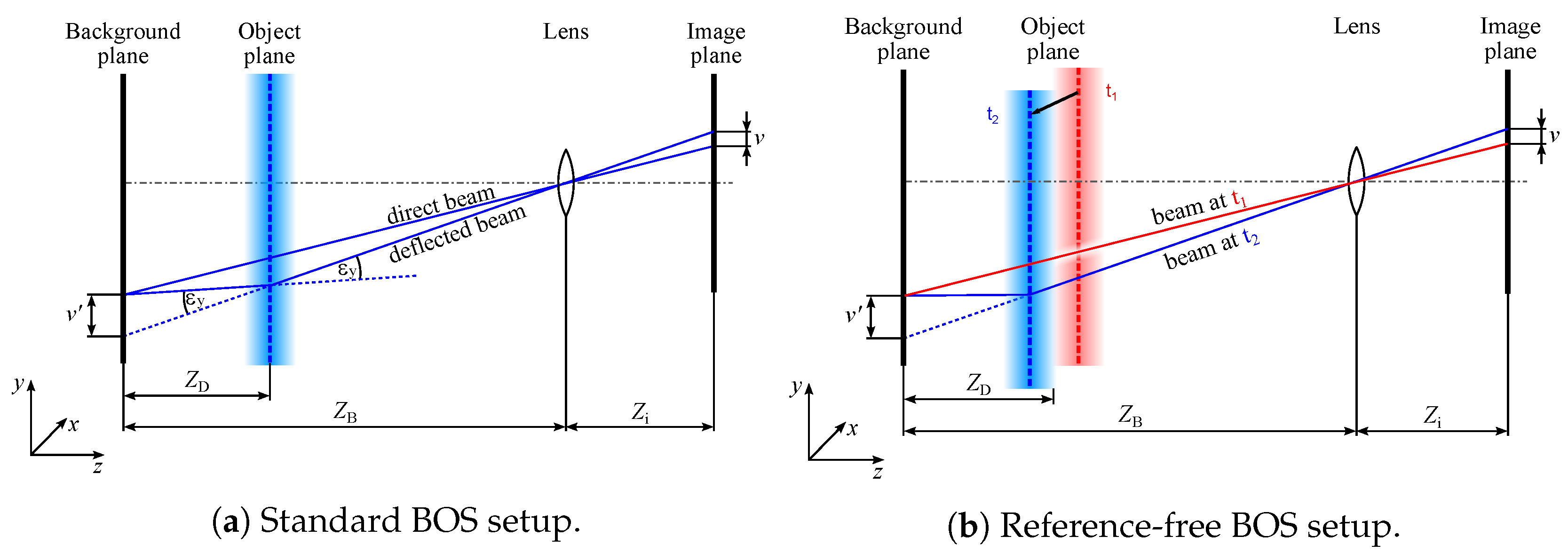
3.2.3. Vortex Visualisation with BOS

Flow visualization based on the Background-Oriented Schlieren method was applied during both free-flight and laboratory experiments in order to assess the possibility of non-intrusive flow topology investigations. Figure 17 depicts corresponding results for the full quadcopter in hover out-of-ground effect during the flight tests (Figure 17a) and of the single rotor laboratory case (Figure 17b). The flight test result was acquired with the remote-controlled camera of a second multicopter flying above and to the side of the primary quadcopter using variations in surface brightness on the tarmac of the test site, as shown in the insert on the top right of the figure. As can be seen in the grayscale image, this natural background structure results in high levels of noise in the depicted divergence of the displacement field due to loss of correlation caused by insufficient contrast and too-large structures in the background. Correspondingly, aerodynamic features are difficult to see in this figure. Dark elliptical curves (as marked by a red box) highlight the positions of the blade tip vortices around the rotors and give an impression of where they are located in space. These tip vortices are the dominant flow features for this case and important for assessing the interactions of the rotor wake with potential atmospheric sensors. They are strongly related to the high-frequency fluctuations measured by the pressure and temperature sensors, as discussed above. In the current case, the maximum visibility of the vortices is below ${180}^{\circ }$, i.e., half a rotor revolution, whereas other studies have been able to visualize vortices of similarly sized vehicles for significantly longer, e.g., for up to 3.5 rotor revolutions [48]. A parallel test with a single rotor in the laboratory is shown in Figure 17b, depicting a side view of one rotor arm, motor and propeller blade. An actively illuminated, high-contrast retro-reflective background was used for this study, leading to significantly reduced background noise and better resolution of the tip vortices, which also appear as darker lines in the divergence field. The visibility of the tip vortices is significantly increased here to well beyond ${360}^{\circ }$, i.e., over one full rotor rotation. Additionally, vortex breakup (below the rotor arm) and secondary vortices (to the right side above the rotor arm) are visible, as well as thermal Schlieren directly to the right of the motor. Relative positions and the interaction of the vortices with the rotor arm can therefore be clearly assessed from this data set, highlighting that the rotor produces vortices that are sufficiently strong for visualization with the BOS method. Based on this kind of measurement, relative vortex strengths and positions in space can be derived, giving valuable information about the overall flow field topology complementary to the point-based pressure and temperature measurements. Future in-flight investigations with the BOS method will employ more suitable background structures as well as a further optimized imaging setup to highly improve the measurement sensitivity and resolve features of the rotor wakes in more detail.

3.2.4. Discussion of Comparison of CFD and Flight Test Data

A detailed comparison between pressure and temperature signals obtained from flight tests and from numerical flow simulations was made in the previous sections. This comparison showed that some of the general aerodynamic effects are well resolved in both test cases, while other details differ and require closer examination. From these initial studies, certain critical conclusions and recommendations can be derived to further improve this comparison.

The main challenge of the CFD simulations is the proper spatial resolution of the tip vortices and preventing early diffusion of the corresponding vorticity. Beyond the already implemented adaptive mesh refinement, this may require the application of scale-resolving hybrid RANS/LES (Large Eddy Simulation) schemes. In these types of schemes, the turbulent flow away from the walls is directly resolved on the computational grid with LES, while the smaller turbulent structures in the flow close to the walls are covered by RANS with a sub-grid scale turbulence model, to properly resolve all relevant flow features. A detailed comparison with flight test data further requires a more precise monitoring of the ambient conditions, as well as modelling of the intrusive sensor geometry and data extraction over a certain spatial volume to model the effects of the physical sensor.

The acquired flight test data reveal that further improvements in the test setup are also possible, to reduce the interaction of rotor near-field and sensor mounts, increase the recording time and number of run repetitions, as well as closely monitor the state of the rotorcraft and all four propellers to more precisely determine the flight conditions. Especially for the temperature sensors, the acquired data indicate that the experimental setup could be tailored further to resolve the small rotor-induced temperature fluctuations, or change the sensor layout to be even less sensitive to the rotor effects and only resolve atmospheric distortions. The outcomes of these further investigations would have implications for the optimal sensor setup, positioning, and general distribution of the scientific payload of meteorological multicopters.

3.3. Structure Deformation Results

The few presently implemented vibration and strain measurement locations are used to obtain the first qualitative insights into the structural-dynamic behavior of this quadcopter system but are, by far, not sufficient for a modal analysis. Despite an apparent orthotropic symmetry, slight deviations from the mean stiffness and mass distribution can be assumed for all four rotor arms and the centre section. Furthermore, as the rotors are not phase-synchronised, a complex vibration behavior and pronounced beats are to be expected. Rotational deformation of the rotor arms might cause cross-coupling to the linear accelerometers, which are offset in relation to the rotor arm elastic axes. Example results of the vibration and force measurements are presented and discussed in the following sections.

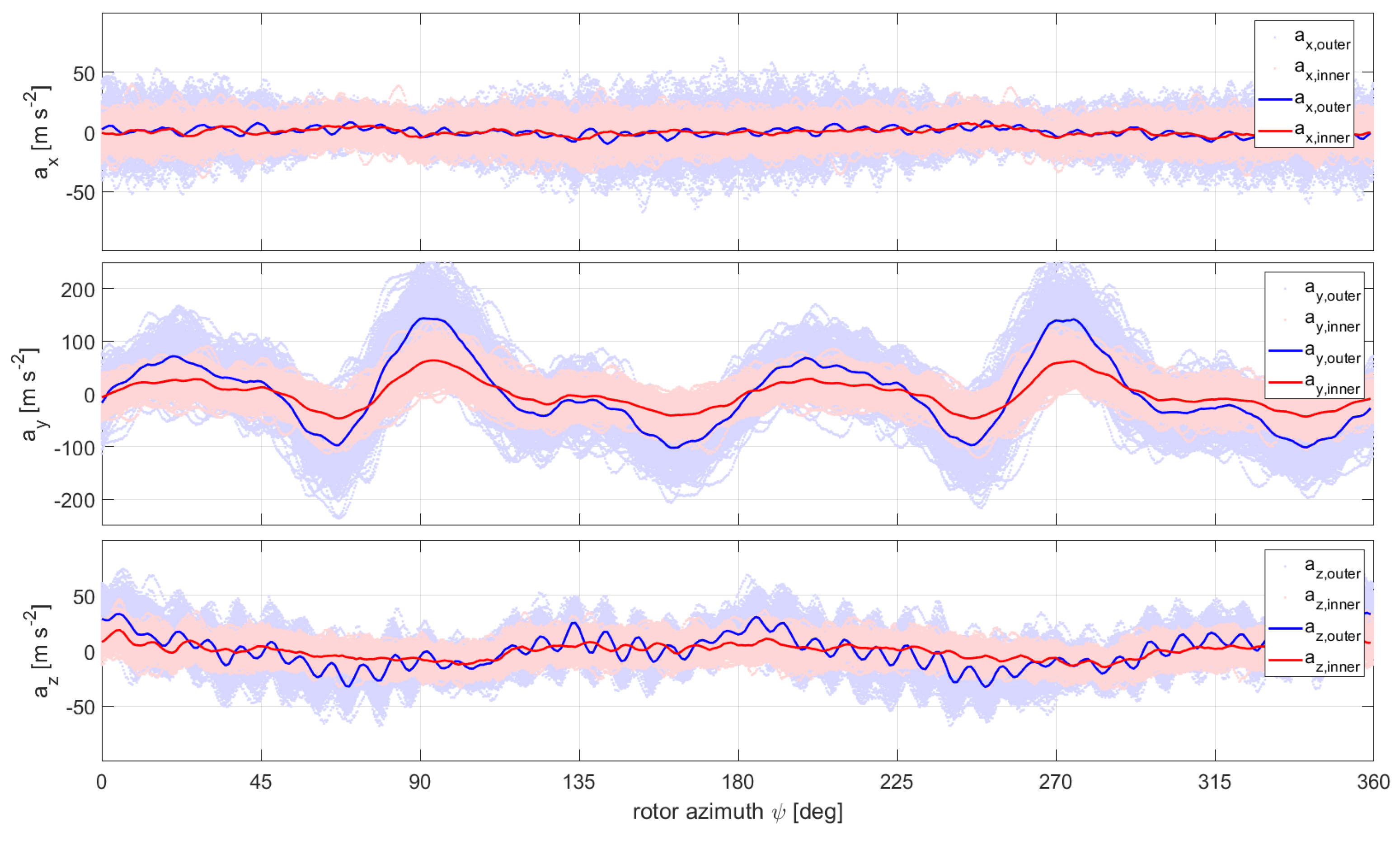
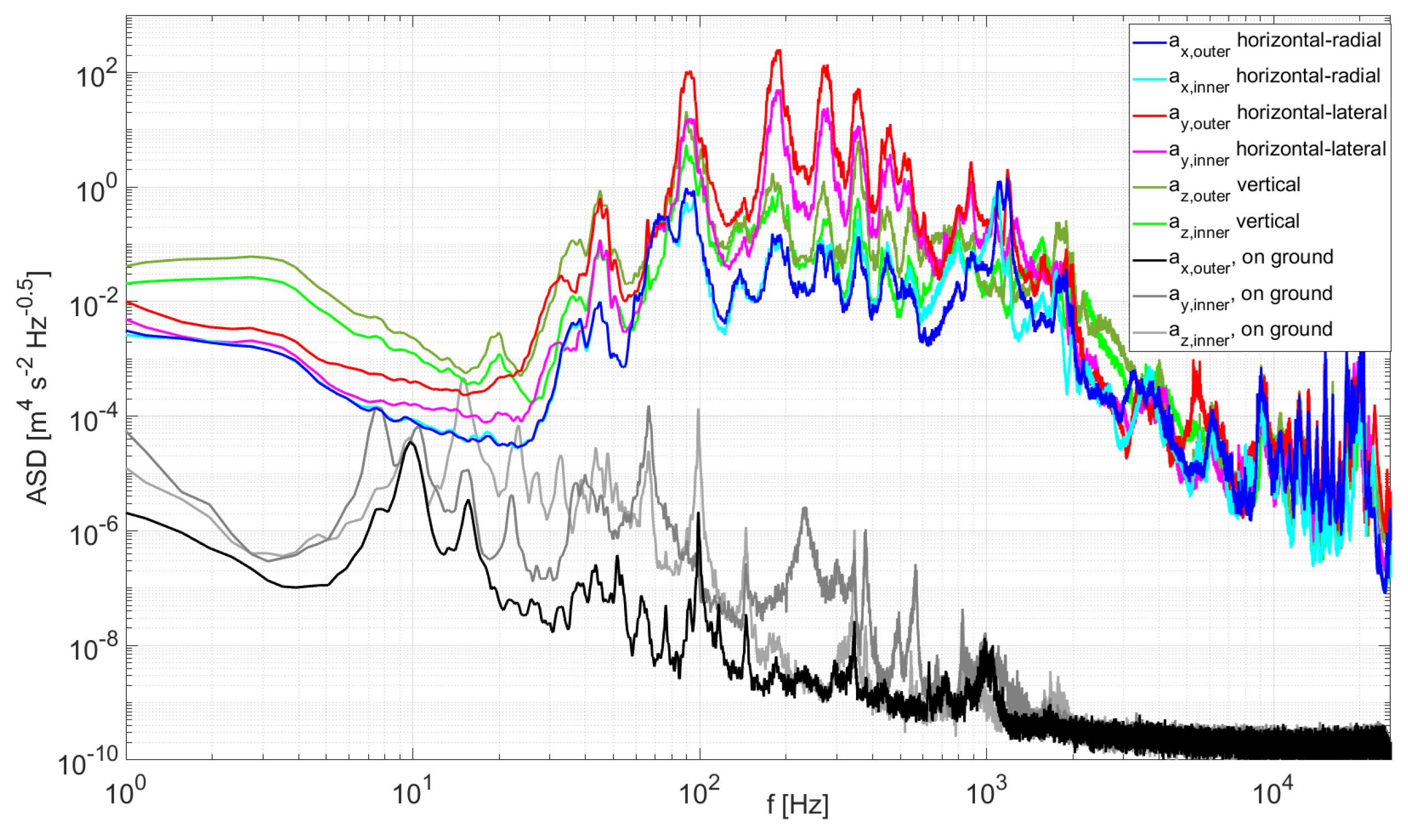
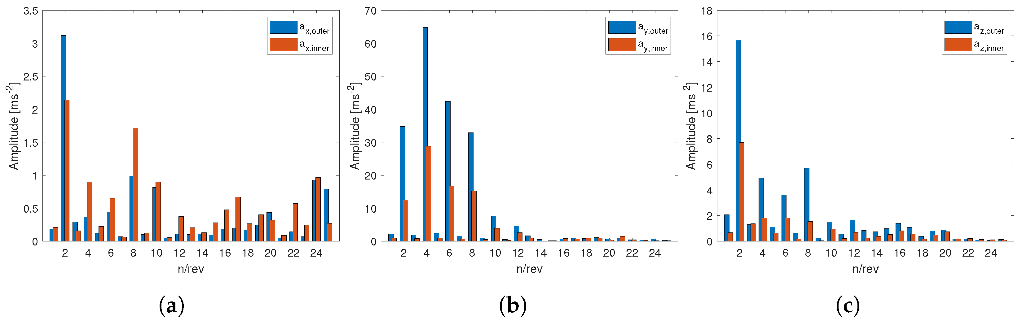
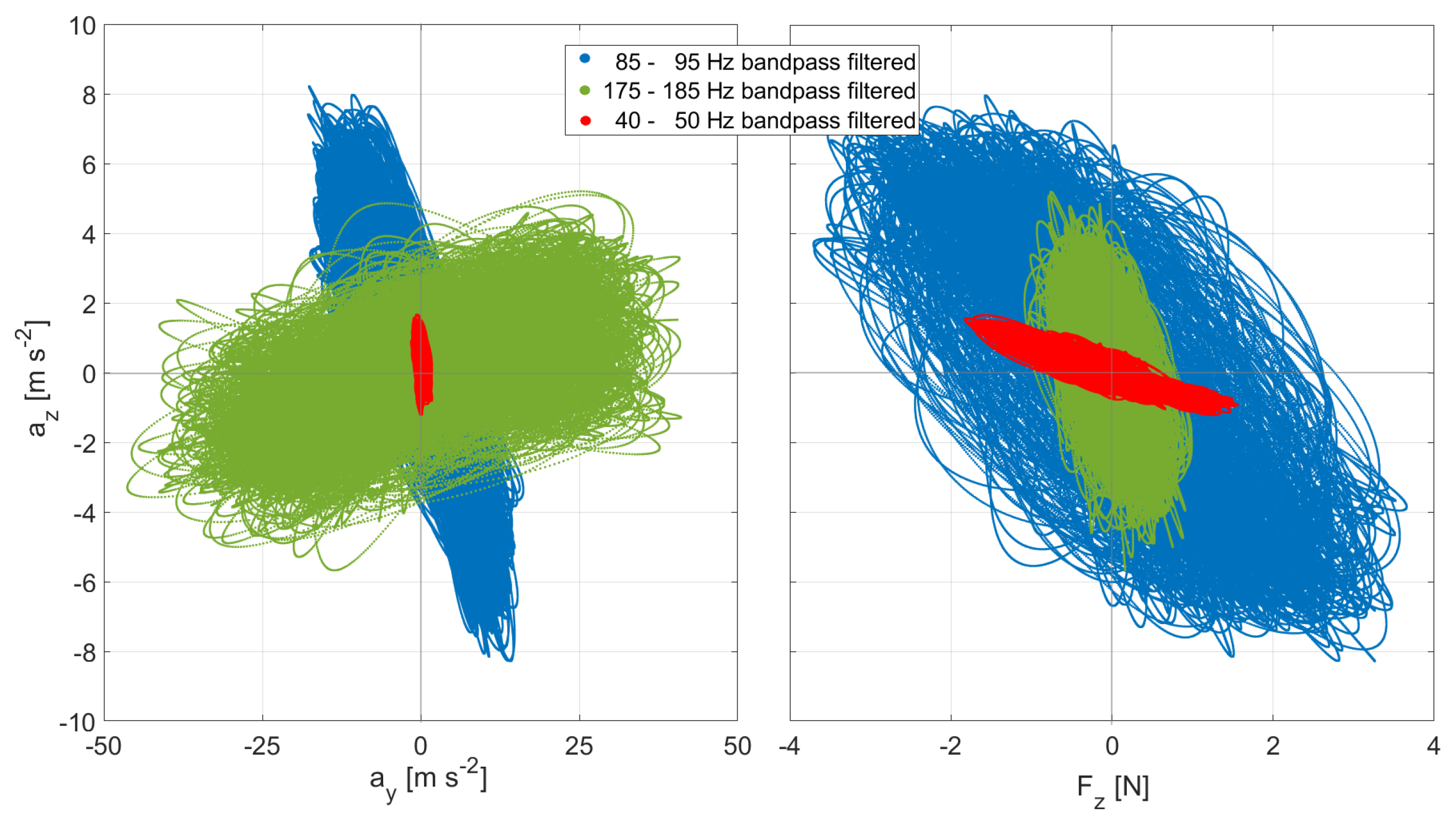
3.3.1. Vibration Measurement Results

Time series plots show the range of structural accelerations that can occur. However, to understand excitation sources, the spectral behavior is considered, in particular harmonically decomposed signal components based on the periodic propeller rotation. The measured voltages of the accelerometers were converted to accelerations in the three coordinate directions using factory calibration factors. Figure 18 shows phase-resolved accelerations in the x (horizontal radial), y (horizontal lateral) and z (vertical) direction of the instrumented rotor arm for a total duration of 4 s in quasi-steady hover (Flight 15). Besides the individual measurement data, which are shown as light colored curves for the two radial sensor positions, ensemble-averaged results are superimposed as darker curves. The individual data reveal a periodic acceleration pattern that does persist for the averaged curves. The average data exhibit a complex signal that is the superposition of different eigenmodes and the superimposed excitations due to all four rotors.

To explain these signals in detail, all excitation sources must be observed and a modal characterization of the whole airframe must be performed, which is a complex task due to the large number of required measurement channels and sensors. This is beyond the scope of the current investigation. It is also worth noting that the peak amplitudes of the averaged acceleration signals are about a factor of two smaller than the ultimate accelerations experienced in individual measurement cycles, highly underestimating the peak accelerations experienced by the system.

Figure 19 transfers the temporal acceleration behavior into the frequency domain and Figure 20 provides the corresponding harmonic decomposition. The gray-scale curves at the bottom of Figure 19 correspond to the background measurements also presented in Figure 5a, and show a sufficient signal-to-noise ratio above 30 Hz. The local maximum in the spectral distribution of the in-flight data at 1/rev (45 Hz) indicates a propeller imbalance (Figure 19). Cross-examination of the harmonic decomposition (Figure 20b), however, reveals that the corresponding amplitudes are relatively small and therefore negligible, showing the importance of different modes of data analysis. In general, the acceleration amplitudes are highest in the horizontal lateral direction, followed by the vertical direction. The corresponding accelerations are higher at the outer sensor position than at the inner one, indicating predominant excitation of bending deformations of the rotor arm. The excitation due to each propeller blade wake at 90 Hz or 2/rev can be identified as the main source of airframe vibrations, both directly at 2/rev frequency and also at its even higher-harmonics. Especially for the horizontal lateral accelerations $a_y$, the 4/rev frequency dominates the spectrum, reaching the highest acceleration amplitudes of around 65 m s${}^{-2}$ for the outer position (Figure 20b). This particular frequency component is also clearly visible in the acceleration signal shown in Figure 18. Note that differences in peak amplitudes occur due to the added contributions of different frequency components.

Figure 18 shows the range of accelerations that can occur in the combined signal, but the contributions of each of the harmonically decomposed signal components are revealed in Figure 20. The maximum acceleration in Figure 18 is the addition of the accelerations of the different harmonically decomposed signals shown in Figure 20. This demonstrates that the spectral behavior of accelerations has to be taken into account for identifying the potential impact on the platform and sensors.

The measured accelerations in the x direction appear in view of Figure 20a probably as an artefact of the sensor positions outside the elastic axes of the rotor arm, which altogether underlines the already mentioned necessity of a full modal analysis.

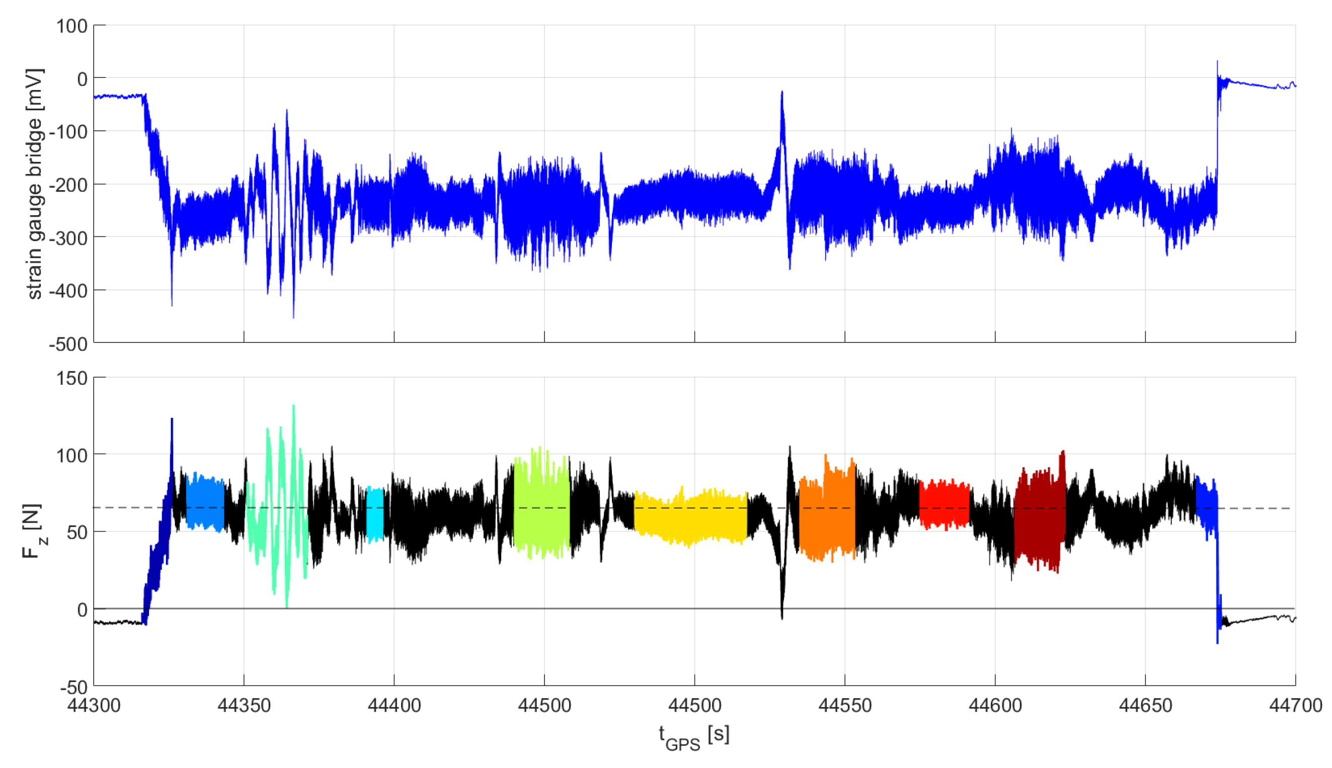
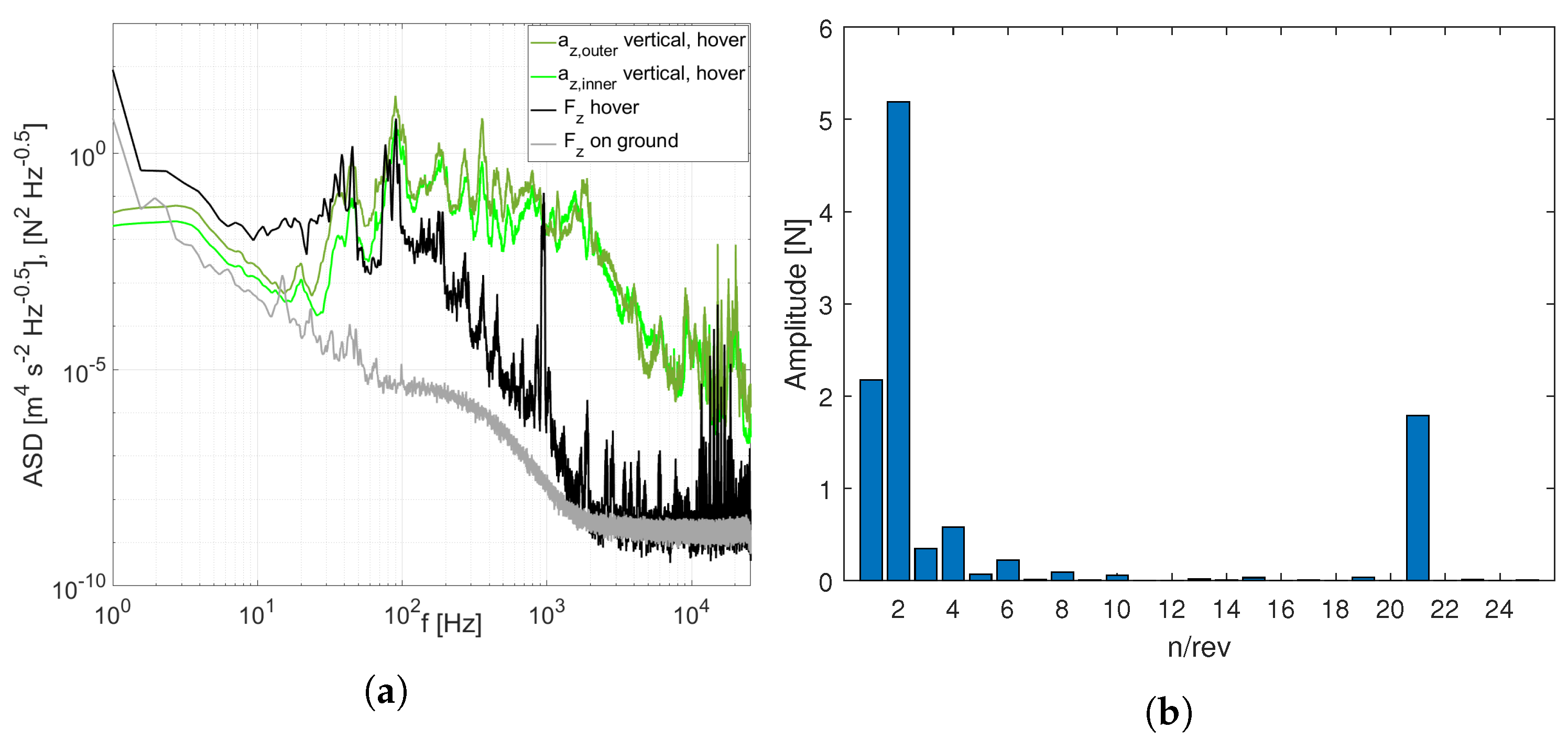
3.3.2. Force Measurement Results

The measured bridge voltage of the vertical strain gauge on the rotor arm was converted to a force using the known weight of the rotor arm and propeller at zero rotation speed on the ground, and assuming an average force in flight equaling one quarter of the total weight force. The conversion is illustrated in Figure 21 from the raw voltage signal, which is assumed to have a linear relationship with force and calibrated by a two-point calibration, to the calculated force of Flight 15. Different flight maneuvers are color-coded according to the flight sequences labelled in Figure 8. The data highlight the different load characteristics obtained for these maneuvers, e.g., relatively homogeneous loading with moderate fluctuations during hover phases (blue, light blue) and fast forward flight (yellow, red). High load fluctuations were measured during harsh alternating clockwise and counterclockwise yaw maneuvers, e.g., at ca. 44,360 s (turquoise) and at three additional points in time later in the recorded signal. These intentionally flown maneuvers are carried out by imbalancing the yaw moment of the counter-rotating propellers through different commanded speeds of rotation. In this arrangement, the decreasing lift of the pair of slowed down propellers must be compensated by increasing the speed of rotation of the other pair of propellers. Based on a design thrust-to-weight ratio of 2.3 and no thrust reversal possible, it can be assumed that the multicopter was close to its maximum yaw rate during this maneuver, and also close to its upper lift limit at peak yaw rate. The examined data show that measuring the effective force at representative locations of the structure provides deeper insights into the flight mechanical characteristics of the quadcopter.

Besides the relevance for flight mechanical questions, this kind of measurement can also be used to obtain in-flight dynamic load cycles for life cycle testing of components. The spectra in Figure 22a show a correlation of the vertical acceleration and the corresponding vertical force for the chosen 4 s hover segment of the same flight. The 2nd order low-pass filter with −3 dB at 250 Hz, which is hardware-implemented and results in an increasing amplitude underestimation from 100 Hz upward, was not corrected but must be kept in mind. In addition, transferring a static calibration to a dynamic measurement must be done with caution because the strain-measuring element is large compared to the elastic fine structures of the carbon fibre rotor arm tube and applied near the tube connector to the centre section. A comparison with calculated strains due to deformations derived from measured accelerations requires a sufficiently good elastic model, which is recommended for future investigations. A harmonic decomposition of the corresponding vertical force signal is added in Figure 22b. The low-pass filtering is also apparent in the harmonic decomposition data in Figure 22b, where the initial frequencies of 1/rev (45 Hz) and 2/rev (90 Hz) are still properly captured but amplitudes above are significantly reduced, in contrast to the harmonic decomposition of the corresponding vertical acceleration signal in Figure 20c that features distinct peaks in the even harmonics up to 8/rev. The electromagnetic interference caused by the motors is again clearly visible in both figures in the form of a broad increase in signal power between 900 Hz and 1000 Hz for the vertical accelerations, a sharp peak for the vertical force and a distinct 21/rev amplitude peak in the harmonic decomposition chart. Finally, the data highlight the effect of a propeller blade imbalance in the moderately high 1/rev peak present both in the force and acceleration signals. Together with the higher-harmonic frequency content, these structural vibrations are important to quantify and consider for the measurement systems, as previous studies have shown that they can affect the readings of certain sensor systems [27].

3.3.3. Phase Considerations between Acceleration and Force Measurements

The previously shown correlation between the accelerations of the rotor arm and the vertical forces is extended in this section by a further illustration. Figure 23 shows the vertical accelerations $a_z$ cross-plotted against the horizontal lateral acceleration $a_y$ and the vertical force $F_z$ for a hover phase. The signal is split into different frequency bands by bandpass-filtering the accelerations and force at the rotor speed of rotation (1/rev, 45 Hz) and its second (90 Hz) and fourth (180 Hz) higher harmonics. The different band-limited phase plots exhibit distinct interactions between the accelerations and forces, some of which could be linearly approximated. However, the representation of the full data set allows deeper insights into the complexity of the vibration modes of the overall system. A full vibration analysis of the system would require more comprehensive instrumentation on at least all four rotor arms and appropriate modal analysis, which was not the goal of the present preliminary test. Future test flights may be instrumented accordingly to distinguish between the contributions of the four rotors to the overall modal structural response.

4. Conclusions

This study investigated the interaction of propeller-induced flow on a multicopter with onboard measurement systems. The measurement systems were described in detail, featuring sensors for investigating the rotor-induced near flow field and the resulting structural vibrations in a frequency range from about 10${}^1$ to 10${}^3$ Hz. The measurement setup utilized existing sensors for pressures, temperatures, accelerations, force, rotor speed, phase, and an existing data acquisition unit without significant adaptions. The measurements were conducted as a secondary objective during the initial full-scale, free-flight test phase of a newly developed quadcopter system. This low-cost early-stage-error approach provided insights into the challenges of these kinds of measurements and analysis as the basis for more thorough investigations. The variable sensor setup was focused on one rotor arm of the quadcopter, assumed to be representative for the full system. The data were analyzed for quasi-stationary hover sections, as the limited number of sensors and flight repetitions did not allow decomposition of the complex system behavior during dynamic flight phases. The results were compared with laboratory measurements of isolated sensors and of an isolated rotor assembly in hover, as well as with numerical flow simulations of an isolated rotor assembly, complementing the analysis of flight test data. The data of a total of 16 flights were analyzed to assess the usability of the sensor setup and to derive basic results, like dominant effects, ensemble-averaged quantities, and spectrally as well as harmonically decomposed characteristics.

The main conclusions of this work and corresponding recommendations for future studies are summarized here:

• General conclusions about the flight tests:

• The limited number of channels necessitated repeated flight tests with different sensor setups. However, this approach is detrimental to the data quality, as the operating conditions cannot be reproduced perfectly between runs due to, e.g., changing weather and manually flown maneuvers. Future investigations should incorporate an improved data acquisition system with more channels, longer flight phases for improved averaging, and monitoring of operating and ambient conditions. Approaches to minimize the atmospheric turbulence, e.g., by flights in the early morning for stable atmospheric stratification, during parts of the trials should be taken into account.
• Only a single rotor arm was instrumented during the flight tests. While this setup already generates initial knowledge of the system’s characteristics, a deeper analysis of structural vibrations requires instrumentation of all four rotor arms.
• Electromagnetic interference was found for multiple of the onboard electric sensors and traced back to the electric drive train of the quadcopter. Harmonic decomposition of the signal proved to be a powerful method for removing this effect from the measurement signals. Electromagnetic shielding should be considered for the structural sensors to reduce these effects in the future.
• The current tests were conducted with a rather high data acquisition rate of 51.2 kHz. This frequency proved to be unnecessarily high for the targeted application and could be reduced in future studies to facilitate data analysis through reduced processing time. A proper investigation is recommended for identifying the new data rate to avoid unintended signal corruption or missing relevant effects.

• Conclusions about the individual onboard sensors:

• A simple and reliable method for determining the rotor speed and phase was implemented and tested. The system could be further improved by adding more markers over the circumference to better resolve unsteady rotor speed fluctuations and slow rotor speeds.
• The applied pressure measurement setup produced meaningful results, adequately resolving dominant effects due to the rotor wake interaction and comparing well with numerical results. However, the physical presence of the sensors and their mounts is believed to influence the local flow and pressure to be measured. Therefore, the sensor setup should be improved to minimize its effect on the flow, and the setup should also be resolved in the numerical flow simulations.
• Mixed results were obtained for the finewire temperature sensors, whose design was not adjusted for this test campaign. The sensors exhibited high robustness and captured some of the propeller-induced effects but the wire layout and corresponding spatial averaging hindered proper resolution of the fine structures in the propeller wake. Future implementations of this sensor type will first strive to properly resolve all features in the near flow field of the multicopter for validation of numerical methods, before identifying designs and placements that make the sensor less sensitive to propeller interference.
• The used accelerometers are highly suitable for this application and provided meaningful results for the accelerations at selected points on the structure. In the future, the sensor positions should be selected based on numerical or experimental modal analysis to further improve the usability of the results.
• The measured vibrations of the rotor arm are largely caused by the interaction of the rotor wake with the rotor arm. The four times higher acceleration in lateral compared to vertical direction results from a low structural rigidity of the center section in the horizontal plane. Based on the measured data, a life cycle testing program for the structure could be derived.
• Strain gauges were successfully applied, and it was shown that low-frequency structural deformations and dynamic loads can be obtained with them. The low-pass filter characteristics should be adjusted to the desired frequency range for future studies. A structural model can be used to further improve the accuracy of the propeller thrust estimation.
• A first application of the Background-Oriented Schlieren method for in-flight visualization of the propeller tip vortices of a quadcopter was attempted based on a camera mounted on a secondary multicopter. The in-flight results did not reach the same quality obtained in the laboratory experiment. This was mainly due to the operational restrictions for the flight tests and unsuitable background structures available at the test site. Based on the laboratory tests, further improvements should be feasible for the in-flight application and will be pursued in the future.

• Comparison with results from laboratory tests and numerical studies:

• The flight tests were accompanied by laboratory tests to isolate different effects on the sensor signals. Tests without propeller flow allowed analyzing the sensors’ electrical characteristics, while laboratory tests with an isolated propeller were conducted to identify propeller-induced effects without atmospheric disturbances. In addition, flow simulations were carried out for the isolated propeller setup to allow comparison of the different approaches. The combined analysis of these results revealed additional findings that were not apparent in the flight test data alone, therefore showing once again the need for a multi-modal approach in order to gain an overall understanding of the involved flow physics and their interactions with the structure and the sensors on multicopters.
• The comparison between flight test data and numerical simulation results showed that certain flow effects matched decently well between both data sets, like the dominant blade vortices interacting with the rotor arm and sensors around it. This means that relevant parts of the unsteady flow close to the propeller can basically be reproduced by the implemented numerical flow simulations for an isolated propeller. Details, however, differed between flight test and simulation, like negative pressure spikes after the vortex interactions or the temporal development of the temperature fluctuations. The main reason for these discrepancies is thought to stem from the sensor and mounting geometries that were not modelled in the simulation but affect the flow and lead to spatially averaging effects. Further improvements are sought by more accurately determining the ambient and operating conditions during the flight tests and including the sensor geometries in future numerical flow simulations.
• A numerical model of the rotor arm structure to assess elastic and modal properties was not part of this investigation but will undoubtedly be very valuable for future investigations.

• Implications for scientific payload sensors

The current work is an initial step towards fully characterizing the effects of the propeller-induced flow and structural vibrations on the measurement uncertainties of atmospheric sensors aboard a multicopter. Based on the presented preliminary results, no comprehensive set of recommendations can yet be made about optimal positioning or necessary modifications of flow sensors for application on multicopters. Future work will include the design of flight experiments to properly characterize the propeller’s effect on in-flight measurements with dedicated sensors of suitable design and placement. Based on this outcome, best practices will be derived for the optimal design and placement of sensors for unbiased atmospheric measurements.

References

1. Lampert, A.; Pätzold, F.; Asmussen, M.; Lobitz, L.; Krüger, T.; Rausch, T.; Sachs, T.; Wille, C.; Sotomayor Zakharov, D.; Gaus, D.; et al. Studying boundary layer methane isotopy and vertical mixing processes at a rewetted peatland site using an unmanned aircraft system. Atmos. Meas. Tech. 2020, 13, 1937–1952. [Google Scholar] [CrossRef]
2. Martin, S.; Bange, J.; Beyrich, F. Meteorological profiling of the lower troposphere using the research UAV “M2AV Carolo”. Atmos. Meas. Tech. 2011, 4, 705–716. [Google Scholar] [CrossRef]
3. Alamouri, A.; Lampert, A.; Gerke, M. An Exploratory Investigation of UAS Regulations in Europe and the Impact on Effective Use and Economic Potential. Drones 2021, 5, 63. [Google Scholar] [CrossRef]
4. Van den Kroonenberg, A.C.; Martin, T.; Buschmann, M.; Bange, J.; Vörsmann, P. Measuring the Wind Vector Using the Autonomous Mini Aerial Vehicle M2AV. J. Atmos. Ocean. Technol. 2008, 25, 1969–1982. [Google Scholar] [CrossRef]
5. Reuder, J.; Brisset, P.; Jonassen, M.; Mayer, S. The Small Unmanned Meteorological Observer SUMO: A new tool for atmospheric boundary layer research. Meteorol. Z. 2009, 18, 141–147. [Google Scholar] [CrossRef]
6. Elston, J.; Argrow, B.; Stachura, M.; Weibel, D.; Lawrence, D.; Pope, D. Overview of Small Fixed-Wing Unmanned Aircraft for Meteorological Sampling. J. Atmos. Ocean. Technol. 2015, 32, 97–115. [Google Scholar] [CrossRef]
7. Lampert, A.; Pätzold, F.; Jiménez, M.A.; Lobitz, L.; Martin, S.; Lohmann, G.; Canut, G.; Legain, D.; Bange, J.; Martínez-Villagrasa, D.; et al. A study of local turbulence and anisotropy during the afternoon and evening transition with an unmanned aerial system and mesoscale simulation. Atmos. Chem. Phys. 2016, 16, 8009–8021. [Google Scholar] [CrossRef]
8. Altstädter, B.; Platis, A.; Wehner, B.; Scholtz, A.; Wildmann, N.; Hermann, M.; Käthner, R.; Baars, H.; Bange, J.; Lampert, A. ALADINA—An unmanned research aircraft for observing vertical and horizontal distributions of ultrafine particles within the atmospheric boundary layer. Atmos. Meas. Tech. 2015, 8, 1627–1639. [Google Scholar] [CrossRef]
9. Lee, J.; Park, J.; Kim, J. Vertical measurement of equivalent black carbon concentration at low altitude. Appl. Sci. 2020, 10, 5142. [Google Scholar] [CrossRef]
10. Wu, C.; Liu, B.; Wu, D.; Yang, H.; Mao, X.; Tan, J.; Liang, Y.; Sun, J.Y.; Xia, R.; Sun, J. Vertical profiling of black carbon and ozone using a multicopter unmanned aerial vehicle (UAV) in urban Shenzhen of South China. Sci. Total Environ. 2021, 801, 149689. [Google Scholar] [CrossRef]
11. Chiba, T.; Haga, Y.; Inoue, M.; Kiguchi, O.; Nagayoshi, T.; Madokoro, H.; Morino, I. Measuring regional atmospheric CO2 concentrations in the lower troposphere with a non-dispersive infrared analyzer mounted on a UAV, Ogata Village, Akita, Japan. Atmosphere 2019, 10, 487. [Google Scholar] [CrossRef]
12. Barchyn, T.E.; Hugenholtz, C.H.; Fox, T.A. Plume detection modeling of a drone-based natural gas leak detection system. Elem. Sci. Anthr. 2019, 7, 41. [Google Scholar] [CrossRef]
13. Villa, T.F.; Gonzalez, F.; Miljievic, B.; Ristovski, Z.D.; Morawska, L. An Overview of Small Unmanned Aerial Vehicles for Air Quality Measurements: Present Applications and Future Prospectives. Sensors 2016, 16, 1072. [Google Scholar] [CrossRef] [PubMed]
14. Lampert, A.; Altstädter, B.; Bärfuss, K.; Bretschneider, L.; Sandgaard, J.; Lobitz, L.; Asmussen, M.; Damm, E.; Käthner, R.; Krüger, T.; et al. Unmanned Aerial Systems for Investigating the Polar Atmospheric Boundary Layer—Technical Challenges and Examples of Applications. Atmosphere 2020, 11, 416. [Google Scholar] [CrossRef]
15. Bärfuss, K.; Dirksen, R.; Schmithüsen, H.; Bretschneider, L.; Pätzold, F.; Bollmann, S.; Panten, P.; Rausch, T.; Lampert, A. Drone-Based Atmospheric Soundings up to an Altitude of 10 km - Technical Approach towards Operations. Drones 2022, 6, 404. [Google Scholar] [CrossRef]
16. Bärfuss, K.B.; Schmithüsen, H.; Lampert, A. Drone-based meteorological observations up to the tropopause. Atmos. Meas. Tech. Discuss. 2023, 16, 3739–3765. [Google Scholar] [CrossRef]
17. Simma, M.; Mjøen, H.; Boström, T. Measuring Wind Speed Using the Internal Stabilization System of a Quadrotor Drone. Drones 2020, 4, 23. [Google Scholar] [CrossRef]
18. Thielicke, W.; Hübert, W.; Müller, U.; Eggert, M.; Wilhelm, P. Towards accurate and practical drone-based wind measurements with an ultrasonic anemometer. Atmos. Meas. Tech. 2021, 14, 1303–1318. [Google Scholar] [CrossRef]
19. Chilson, P.B.; Bell, T.M.; Brewster, K.A.; Britto Hupsel de Azevedo, G.; Carr, F.H.; Carson, K.; Doyle, W.; Fiebrich, C.A.; Greene, B.R.; Grimsley, J.L.; et al. Moving towards a Network of Autonomous UAS Atmospheric Profiling Stations for Observations in the Earth’s Lower Atmosphere: The 3D Mesonet Concept. Sensors 2019, 19, 2720. [Google Scholar] [CrossRef]
20. De Boer, G.; Diehl, C.; Jacob, J.; Houston, A.; Smith, S.W.; Chilson, P.; Schmale, D.G.; Intrieri, J.; Pinto, J.; Elston, J.; et al. Development of Community, Capabilities, and Understanding through Unmanned Aircraft-Based Atmospheric Research—The LAPSE-RATE Campaign. Bull. Am. Meteorol. Soc. 2020, 101, 684–699. [Google Scholar] [CrossRef]
21. Greene, B.R.; Segales, A.R.; Waugh, S.; Duthoit, S.; Chilson, P.B. Considerations for temperature sensor placement on rotary-wing unmanned aircraft systems. Atmos. Meas. Tech. 2018, 11, 5519–5530. [Google Scholar] [CrossRef]
22. Smith, B.; John, G.; Stark, B.; Christensen, L.E.; Chen, Y.Q. Applicability of Unmanned Aerial Systems for Leak Detection. In Proceedings of the International Conference on Unmanned Aircraft Systems (ICUAS), Arlington, VA, USA, 7–10 June 2016. [Google Scholar]
23. Brosy, C.; Krampf, K.; Zeeman, M.; Wolf, B.; Junkermann, W.; Schäfer, K.; Emeis, S.; Kunstmann, H. Simultaneous multicopter-based air sampling and sensing of meteorological variables. Atmos. Meas. Tech. 2017, 10, 2773–2784. [Google Scholar] [CrossRef]
24. Shah, A.; Allen, G.; Pitt, J.R.; Ricketts, H.; Williams, P.I.; Helmore, J.; Finlayson, A.; Robinson, R.; Kabbabe, K.; Hollingsworth, P.; et al. A Near-Field Gaussian Plume Inversion Flux Quantification Method, Applied to Unmanned Aerial Vehicle Sampling. Atmosphere 2019, 10, 396. [Google Scholar] [CrossRef]
25. Greene, B.R.; Segales, A.R.; Bell, T.M.; Pillar-Little, E.A.; Chilson, P.B. Environmental and Sensor Integration Influences on Temperature Measurements by Rotary-Wing Unmanned Aircraft Systems. Sensors 2019, 19, 1470. [Google Scholar] [CrossRef] [PubMed]
26. Barbieri, L.; Kral, S.T.; Bailey, S.C.C.; Frazier, A.E.; Jacob, J.D.; Reuder, J.; Brus, D.; Chilson, P.B.; Crick, C.; Detweiler, C.; et al. Intercomparison of Small Unmanned Aircraft System (sUAS) Measurements for Atmospheric Science during the LAPSE-RATE Campaign. Sensors 2019, 19, 2179. [Google Scholar] [CrossRef] [PubMed]
27. Lampert, A.; Hartmann, J.; Pätzold, F.; Lobitz, L.; Hecker, P.; Kohnert, K.; Larmanou, E.; Serafimovich, A.; Sachs, T. Comparison of Lyman-alpha and LI-COR infrared hygrometers for airborne measurement of turbulent fluctuations of water vapour. Atmos. Meas. Tech. 2018, 11, 2523–2536. [Google Scholar] [CrossRef]
28. Yoon, S.; Diaz, P.V.; Boyd, D.D., Jr.; Chan, W.M.; Theodore, C.R. Computational Aerodynamic Modeling of Small Quadcopter Vehicles. In Proceedings of the American Helicopter Society 73rd Annual Forum, Fort Worth, TX, USA, 8–11 May 2017. [Google Scholar]
29. Wang, Z.; Henricks, Q.; Zhuang, M.; Pandey, A.; Sutkowy, M.; Harter, B.; McCrink, M.; Gregory, J. Impact of Rotor–Airframe Orientation on the Aerodynamic and Aeroacoustic Characteristics of Small Unmanned Aerial Systems. Drones 2019, 3, 56. [Google Scholar] [CrossRef]
30. Ghirardelli, M.; Kral, S.T.; Müller, N.C.; Hann, R.; Cheynet, E.; Reuder, J. Flow Structure around a Multicopter Drone: A Computational Fluid Dynamics Analysis for Sensor Placement Considerations. Drones 2023, 7, 467. [Google Scholar] [CrossRef]
31. Suchanek, G.; Filipek, R.; Golas, A. Design and Implementation of a Particulate Matter Measurement System for Energy-Efficient Searching of Air Pollution Sources Using a Multirotor Robot. Energies 2023, 16, 2959. [Google Scholar] [CrossRef]
32. Bretschneider, L.; Schlerf, A.; Baum, A.; Bohlius, H.; Buchholz, M.; Düsing, S.; Ebert, V.; Erraji, H.; Frost, P.; Käthner, R.; et al. MesSBAR—Multicopter and Instrumentation for Air Quality Research. Atmosphere 2022, 13, 629. [Google Scholar] [CrossRef]
33. Schlerf, A.; Baum, A.; Bohlius, H.; Bretschneider, L.; Buchholz, M.; Del, A.; Düsing, S.; Ebert, V.; Kim, M.E.; Erraji, H.; et al. Multikopter als fliegende Luftschadstoffmessstationen? Immissionsschutz 2022, 3, 121–129. [Google Scholar] [CrossRef]
34. Bärfuss, K.; Pätzold, F.; Altstädter, B.; Kathe, E.; Nowak, S.; Bretschneider, L.; Bestmann, U.; Lampert, A. New Setup of the UAS ALADINA for Measuring Boundary Layer Properties, Atmospheric Particles and Solar Radiation. Atmosphere 2018, 9, 28. [Google Scholar] [CrossRef]
35. Pätzold, F.; Schlerf, A.; Bretschneider, L.; Bauknecht, A. Multicopter In-Flight Measurement Data of Flow Field and Structure States. Data Set. Available online: https://leopard.tu-braunschweig.de/receive/dbbs_mods_00070168 (accessed on 21 July 2023).
36. Kulite Semiconductor Products, Inc.: Miniature Ruggedized Pressure Transducer XT-190 (M) Series, Data Sheet, 1 p. 2018. Available online: https://kulite.com/products/product-advisor/product-catalog/miniature-ruggedized-pressure-transducer-xt-190m (accessed on 20 March 2023).
37. Richard, H.; Raffel, M. Principle and applications of the background oriented schlieren (BOS) method. Meas. Sci. Technol. 2001, 12, 1576–1585. [Google Scholar] [CrossRef]
38. Venkatakrishnan, L.; Meier, G.E.A. Density measurements using the Background Oriented Schlieren technique. Exp. Fluids 2004, 37, 237–247. [Google Scholar] [CrossRef]
39. Bauknecht, A.; Merz, C.B.; Raffel, M.; Landolt, A.; Meier, A.H. Blade-Tip Vortex Detection in Maneuvering Flight Using the Background-Oriented Schlieren Technique. J. Aircr. 2014, 51, 2005–2014. [Google Scholar] [CrossRef]
40. Bauknecht, A.; Merz, C.B.; Raffel, M. Airborne visualization of helicopter blade tip vortices. J. Vis. 2016, 20, 139–150. [Google Scholar] [CrossRef]
41. Hargather, M.J.; Settles, G.S. Natural-background-oriented schlieren imaging. Exp. Fluids 2010, 48, 59–68. [Google Scholar] [CrossRef]
42. Sanchez-Cuevas, P.; Heredia, G.; Ollero, A. Characterization of the aerodynamic ground effect and its influence in multirotor control. Int. J. Aerosp. Eng. 2017, 17, 1823056. [Google Scholar] [CrossRef]
43. Hunt, J.C.R.; Wray, A.; Moin, P. Eddies, stream, and convergence zones in turbulent flows. In Center for Turbulence Research Report CTR-S88; Stanford University: Stanford, CA, USA, 1988. [Google Scholar]
44. Shih, T.; Liou, W.; Shabbir, A.; Yang, Z.; Zhu, J. A New k-epsilon Eddy Viscosity Model for High Reynolds Number Turbulent Flows. Comput. Fluids 1995, 10, 227–238. [Google Scholar] [CrossRef]
45. Cabezón, D.; Sanz, J.; Martí, I.; Crespo, A. CFD modelling of the interaction between the Surface Boundary Layer and rotor wake. Comparison of results obtained with different turbulence models and mesh strategies. In Proceedings of the European Wind Energy Conference and Exhibition (EWEC), Marseille, France, 16–19 March 2009; pp. 1–7. [Google Scholar]
46. Mohamed, M.H. Performance investigation of H-rotor Darrieus turbine with new airfoil shapes. Energy 2012, 47, 522–530. [Google Scholar] [CrossRef]
47. Chue, S.H. Pressure probes for fluid measurements. Prog. Aerosp. Sci. 1975, 16, 147–223. [Google Scholar] [CrossRef]
48. Bauknecht, A.; Schwarz, C.; Raffel, M.; Mailänder, S. Flow Measurement Techniques for Rotor Wake Characterization on Free-Flying Helicopters in Ground Effect. In Proceedings of the AIAA Scitech Forum, San Diego, CA, USA, 7–11 January 2019; pp. 1–19. [Google Scholar] [CrossRef]
Figure 1. Photograph of the quadcopter during a flight test on 2 March 2021.
Atmosphere 14 01336 g001
Figure 2. Overview of the measurement systems installed on the multicopter. The small pictures provide more details of the different sensors, and the dots and lines in the corresponding colors indicate the location in the large picture: Temperature sensors (blue), data acquisition (purple), pressure sensors (orange), strain gauges (yellow), accelerometers (green) and phase detection (red).
Atmosphere 14 01336 g002
Figure 3. Sketch of standard and reference-free BOS setup.
Atmosphere 14 01336 g003
Figure 4. Amplitude spectral density (ASD) of two sensors tested in the laboratory. Throughout the article, laboratory measurements are displayed in gray scale, field measurements in colors. (a) Kulite pressure sensors without excitation and excited with air flow from a hot-air gun; (b) Fine wire temperature sensors without excitation and excited with air flow from a hot-air gun.
Atmosphere 14 01336 g004
Figure 5. Amplitude spectral density (ASD) of accelerometer and force sensors on ground with all rotors in standstill but excited by wind and vibration of the ground. (a) 3 of the 6 accelerometer signals without excitation; (b) Force signal without excitation.
Atmosphere 14 01336 g005
Figure 6. Rotor hover test stand for experimental validation data.
Atmosphere 14 01336 g006
Figure 7. Numerical setup with (a) overview of computational domain and (b) close-up view of propeller subdomain.
Atmosphere 14 01336 g007
Figure 8. Example Flight 15 on 30 March 2021, segmented into typical flight phases.
Atmosphere 14 01336 g008
Figure 9. Example results for both rotor speed and phase measurement setups. The upper graphs show the raw voltage signal of the photo diode used for the two different rotor speed measurement setups, the center graphs depict a small subsection of the signal (blue) and the determined rotor phase (propeller azimuth angle in red), and the bottom graphs show the corresponding rotor speed. (a) Flight 1 with first setup; (b) Flight 8 with second improved setup.
Atmosphere 14 01336 g009
Figure 10. Pressure data processing: first panel: Example sensor voltage signal for Flight 8, second panel: scaled to absolute ambient pressure and drift-corrected, third panel: filtered pressure signal, and fourth panel: detail view of third panel.
Atmosphere 14 01336 g010
Figure 11. Pressure data processing: example spectra of the pressure sensors in the laboratory and during an 8 s hovering phase of Flight 8.
Atmosphere 14 01336 g011
Figure 12. Pressure signals over radius and azimuth, extracted at ψ = 18 . 2 position. (a) Flight test data, filtered out motor interference. (b) CFD data.
Atmosphere 14 01336 g012
Figure 13. Harmonic decomposition of pressure signals from CFD and flight test experiments for Flight 9 at 85 % R radial location.
Atmosphere 14 01336 g013
Figure 14. Bandpass-filtered temperature fluctuations for a hover section of Flight 1.
Atmosphere 14 01336 g014
Figure 15. Spectra of Finewire 1 during laboratory tests and during standstill after Flight 3, and of both finewire sensors during a 4 s hovering phase of Flight 3.
Atmosphere 14 01336 g015
Figure 16. Analysis of temperature signals from CFD and flight test experiments for Flight 3 at 87.5 % R radial location. (a) Comparison of phase-averaged temperature signals. (b) Harmonic decomposition of temperature signals.
Atmosphere 14 01336 g016
Figure 17. BOS visualization of rotor tip vortices during hover. (a) Free-flight, unsuitable natural background. (b) Single rotor in laboratory, artificial background.
Atmosphere 14 01336 g017
Figure 18. Measured accelerations (3 body-fixed directions, 2 radial locations) for 4 s hover phase of Flight 15. Light colored: all data; dark colored: averaged data.
Atmosphere 14 01336 g018
Figure 19. Acceleration spectra for 4 s hover phase of Flight 15.
Atmosphere 14 01336 g019
Figure 20. Harmonic decomposition of accelerations at inner and outer position for 4 s hover phase of Flight 15. (a) Horizontal radial accelerations a x . (b) Horizontal lateral accelerations a y . (c) Vertical accelerations a z .
Atmosphere 14 01336 g020
Figure 21. Bridge voltage of vertical strain gauge and calculated vertical force for Flight 15. Thrust sequences are color-coded as labelled in Figure 8. Individual flight phases are marked in different colours: hover phases (blue, light blue), fast forward flight (yellow, red), harsh yaw maneuvers (turquoise).
Atmosphere 14 01336 g021
Figure 22. Analysis of vertical force signal for a 4 s hover phase of Flight 15 compared with vertical accelerations and laboratory case. (a) Spectra of accelerations and force for flight and ground case. (b) Harmonic decomposition of flight test force signal.
Atmosphere 14 01336 g022
Figure 23. Crossplots of bandpass-filtered (bandwidth of ±5 Hz) accelerations and vertical force for a 4 s hover phase of Flight 15.
Atmosphere 14 01336 g023
Disclaimer/Publisher’s Note: The statements, opinions and data contained in all publications are solely those of the individual author(s) and contributor(s) and not of MDPI and/or the editor(s). MDPI and/or the editor(s) disclaim responsibility for any injury to people or property resulting from any ideas, methods, instructions or products referred to in the content.