XCO₂ Fusion Algorithm Based on Multi-Source Greenhouse Gas Satellites and CarbonTracker

Abstract

In view of the urgent need for high coverage and high-resolution atmospheric CO₂ data in the study of carbon neutralization and global CO₂ change research, this study combines the Kriging interpolation and the Triple Collision (TC) algorithm to fuse three XCO₂ datasets, OCO-2, GOSAT, and CarbonTracker, to obtain a 1° × 1° half-monthly average XCO₂ dataset. Through a sub division of the Kriging interpolation, the average coverages of the OCO-2 and GOSAT XCO₂ interpolating datasets are increased by 53.65% and 48.5%, respectively. In order to evaluate the accuracy of the TC fusion dataset, this study used a reliable reference dataset, TCCON data, as the verification data. Through comparative analysis, the MAE of the fusion dataset is 0.6273 ppm, RMSE is 0.7683 ppm, and R² is 0.8279. It can be seen that the combination of Kriging interpolation and TC algorithm can effectively improve the coverage and accuracy of the XCO₂ dataset.

1. Introduction

Since the industrial revolution, the concentration of carbon dioxide (CO₂) in the atmosphere has continued to rise, which is an important factor causing the greenhouse effect [1,2]. In recent years, in order to control the trend of global warming and slow down the gradual increase in atmospheric CO₂ concentration, various countries have formulated corresponding emission reduction measures, but the atmospheric CO₂ concentration is still rising [3]. The sixth assessment report of the IPCC in August 2021 revealed that since the 1970s, the rate of global warming has been higher than that of any 50 years in the past 2000 [4]. In order to realize the great vision of peak CO₂ emission by 2030 and carbon neutralization by 2060, the monitoring of global atmospheric CO₂ concentration is essential.

The traditional CO₂ ground-based network observation can obtain relatively high-precision data, but its sites are few and unevenly distributed, and it is difficult to establish sites in the ocean and other regions, so it is difficult to obtain sufficient observation information. Therefore, it presents a significant challenge to obtain the distribution information of global carbon sources and sinks. With the development of remote sensing technology, greenhouse gas observation satellites have gradually developed and become an important means by which to obtain greenhouse gas data [5,6,7,8,9,10]. Compared with ground-based observation networks, satellite remote sensing observation can cover the Earth’s surface to a great extent, but there are also some deficiencies [11,12]. For example, due to the observation limitations of passive satellites, the atmospheric carbon dioxide column concentration (XCO₂) can only be obtained under weather conditions of no cloud cover or low aerosol concentration [13,14]. Due to the restriction of the solar altitude angle, it is also difficult for satellites to observe effective data in high latitudes. Furthermore, because of the error of the inversion algorithm and the limitation of the Earth’s surface or atmospheric conditions, the obtained CO₂ concentration data has a certain deviation.

In order to meet the needs of climate research, the inversion accuracy of satellite observation XCO₂ needs to be better than 1% [15]. Yang Dongxu proposed a spectral correction method for TANSAT based on the UOL FP algorithm, and verified its XCO₂ inversion product with TCCON data, with an RMSE of 1.59 ppm [16]. Ye Hanhan used the optimization estimation method to retrieve XCO₂, and verified the inversion accuracy of the GF-5 satellite by using the data from TCCON ground sites [17]. The results showed that the inversion accuracy of XCO₂ was 0.67%, but the inversion algorithm had insufficient ability to correct the long-range complex atmospheric interference. Matthias Katzfussa and Noel Cressie proposed to use the Bayesian hierarchical spatio-temporal random effect (STRE) model to process AIRS data and compared it to the real dataset of simulation research and global satellite carbon dioxide measurement, but the model only improved the calculation speed [18]. Reuter used seven CO₂ inversion algorithms of the GOSAT and SCIAMACHY satellites. Assuming that there were few outliers, they chose the median as the value in a grid to generate a global high-precision CO₂ fusion dataset EMMA [19]. However, they did not improve the temporal and spatial resolution of CO₂ data. Nguyenf used the CO₂ data of GOSAT and AIRS, but the method only obtained the CO₂ concentration in the low troposphere [20]. Lili Zhang presented a HASM XCO₂ surface obtained by fusing TCCON measurements with GEOS-Chem model results [21]. David Leslie used the neural network method to estimate XCO₂ data from OCO-2 measurement, but it was very time-consuming to train the model in practical application [22]. Stefan Noël used the Fast atmOspheric traCe gAs retrievaL (FOCAL) algorithm to obtain the results of XCO₂ from GOSAT and GOSAT-2 radiation, but after calculating the collected CO₂ concentration data, they still did not obtain a data product with high precision, high coverage, and high temporal and spatial resolution [23].

In this study, the method of data fusion was selected to combine multiple satellite data, and the uncertainty of data was the key factor to be considered in the process of data fusion. It was necessary to assign reasonable weight to each dataset according to the random error of each dataset. When multi-source data is fused, the random error of data is often weakened according to the best combination scheme, so as to generate an independent dataset with better accuracy. Weighted arithmetic average is a common method to combine multiple datasets. Ideally, the uncertainty evaluation of data needs absolute “truth” as a reference. However, it is difficult to obtain the global truth XCO₂ within the scope of a satellite footprint, and the previous verification is only limited to a few TCCON ground sites. In 1998, Stoffeland [24] developed a data quality evaluation method, triple collision (TC), which can avoid obtaining the “truth value”. This method can objectively estimate the random error of three parallel datasets and is applicable to regional and global scales. It has been widely used in various disciplines. In view of this, this study used the Kriging interpolation method to fill the no-data regions of XCO₂ data products from the GOSAT, OCO-2, and carbontracker models, respectively, measured the uncertainty, and integrated the multi-source products to improve the accuracy, coverage, and spatio-temporal resolution through the TC algorithm.

2. Materials

2.1. OCO-2 Satellite

OCO (Orbiting Carbon Observatory) [25] was originally scheduled to launch in 2009, but failed to reach orbit due to carrier rocket failure. Two weeks later, NASA immediately launched its backup scheme, OCO-2 (Orbiting Carbon observatory-2). OCO-2 is only equipped with a three-band imaging grating-type hyperspectral CO₂ detector. OCO-2 has glint, nadir, or target modes. In nadir mode, the instrument has high spatial resolution by directly observing the Earth and collecting data along the ground orbit. Glint mode can provide a higher signal-to-noise ratio over the ocean, while target mode is mainly used for the calibration of specific ground sites. The dataset OCO-2_L2_Lite_FP 10r used in this paper is from the Goddard Earth Science Data and Information Services Center (GES DISC) (https://disc.gsfc.nasa.gov/datasets/OCO2_L2_Lite_FP_10r/), accessed on 1 December 2021.

2.2. GOSAT Satellite

Launched in January 2009, GOSAT is the first satellite with high spectral resolution and wide spectral coverage, which is specially used to monitor the concentration of major atmospheric greenhouse gases (i.e., CO₂ and CH₄) [26]. At present, there are mainly two sets of GOSAT data, one is the Japan GOSAT algorithm developed by the Japanese team, and the other is the ACOS algorithm developed by NASA. The dataset ACOS_L2_Lite_FP_9r used is from the Goddard Earth Science Data and Information Services Center (GES DISC) (https://disc.gsfc.nasa.gov/datasets/ACOS_L2_Lite_FP_9r/, accessed on 1 December 2021).

2.3. CarbonTracker

NOAA built the world’s first business-oriented global carbon assimilation system CT (CarbonTracker) in 2007. CT is an atmospheric assimilation model used to study the temporal and spatial variation characteristics of carbon flux [27,28]. It is used to estimate the variation in surface CO₂ absorption and release over time. CT includes an ocean module, a fire point module, a fossil fuel module, a land surface ecosystem module, and an atmospheric transmission module. It obtains the best state of each module through the data assimilation method. CT provides an effective scientific and decision-making tool for estimating carbon flux, but it relies too much on surface observation data. In areas with few surface observation data, the accuracy of CT still needs to be improved. In recent years, with the support of the EUROCOM (European atmospheric transport inversion comparison) framework, scientists strive to achieve the accuracy and consistency of regional high-precision carbon flux estimation, so as to provide strong support for the assessment of climate impact. The CT XCO₂ datasets used are from NOAA CT2019B (https://gml.noaa.gov/ccgg/carbontracker/CT2019B/, accessed on 1 December 2021).

The introduction of data from OCO-2, GOSAT and CarbonTracker is shown in

Table 1. Data Introduction.

	OCO-2	GOSAT	CarbonTracker
Start date	6 September 2014	21 April 2009	1 January 2000
End date	up to now	up to now	up to now
Spatial resolution	2.25 km × 1.29 km	10.5 km × 10.5 km	2° × 3°
Time resolution	16 days	3 days	1 day

.

2.4. TCCON Data

TCCON (Total Carbon Column Observing Network) sites adopt ground-based Fourier Transform Spectrometers (FTS), and can detect spectral data in the range of 4000~9000 cm⁻¹ in solar radiation [29]. Among them, there are two CO₂ weak absorption bands, 6220 cm⁻¹ and 6339 cm⁻¹. Compared with satellite detection data, the column concentration data of CO₂, CH₄, N₂O, HF, CO, and H₂O from TCCON are more accurate because the retrieval method can effectively avoid the error impact caused by aerosols and cirrus clouds. Therefore, the XCO₂ data products measured by TCCON have been confirmed as the verification standard of satellite remote sensing data [30,31,32,33,34,35]. The main sites of its site selection are still concentrated in North America and Europe, with few sites in East Asia and Oceania. The TCCON data used in this paper is the GGG2014 version, which were obtained from the TCCON Data Archive (https://TCCON.ornl.gov accessed on 1 December 2021). When the solar zenith angle is below 82°, its XCO₂ error is less than 0.25%. The information of TCCON sites used in this paper is shown in

Table 2. Information of TCCON Sites Used in this Study.

Site Area	Site	Site ID	Longitude/°	Latitude/°
East Asia	Saga, Japan [36]	JS	130.29	33.24
	Tsukuba, Ibaraki, Japan, 125HR [37]	TK	140.12	36.05
North America	Reunion Island (Ile de La Reunion), France [38]	PA	−90.27	45.94
	Lamont, OK, USA [39]	OC	−97.49	36.6
European	Izana, Tenerife, Spain [40]	IZ	16.48	28.3
	Bremen, Germany [41]	BR	8.85	53.1
Oceania	Wollongong, Australia [42]	WG	150.88	−34.41
	Darwin, Australia [43]	DB	130.89	−12.43

.

The XCO₂ products used in this paper are OCO2_L2_Lite_FP. 10R retrieved by the ACOS algorithm, GOSAT ACOS_L2_Lite_FP_9r, and CT2019B covering the period from 2017 to 2018. Due to the coverage of clouds, the scattering and absorption of aerosols in the atmosphere, the spacing of satellite orbits, and the limitations of the inversion algorithm, many observation results are determined as bad-quality data. Therefore, data screening was carried out according to the ACOS use guide, and only the data with “xco2_quality_flag” equal to 1 were used to eliminate the data the quality of which does not meet the requirements of OCO-2 and GOSAT [30].

3. Methods

3.1. Interpolation Algorithm

OCO-2 and GOSAT have a large number of areas without XCO₂ observations, especially in high latitudes, oceans, and other areas. Therefore, based on the Kriging interpolation method [44], this paper realized the filling of these blank areas by combining the inherent change trend in time and space and other relevant characteristics of XCO₂ data. The Kriging interpolation method, also known as the spatial autocovariance optimal interpolation method, obtains the distance range affecting the interpolated points by analyzing the variation distribution of spatial attributes at the spatial position. According to the sampling points within this range, the attribute value of the interpolated points is estimated. This paper adopted the method of ordinary Kriging interpolation.

The sample point to be measured is obtained from the measured value of sample points, and the estimated value of the sample point to be measured is:

$$Z^{\ast }\left(x_0\right)={\displaystyle \sum _{i=1}^n{\lambda }_{i}Z\left(x_i\right)}$$

(1)

where, $\lambda$ ($i$ = 1,2,3…, $n$) is the weight coefficient, which is a set of optimal coefficients that can meet the minimum difference between the estimated value and the real value at the point. The weight coefficient needs to meet the following two conditions: (1) the estimation is unbiased, that is, the mathematical expectation of the deviation is zero; (2) the estimation is optimal, that is, the variance between the estimated value and the actual value is the smallest. As shown in (2).

$$\left\{\begin{array}{l}E\left({\widehat{z}}_o-z_o\right)=0\\ \underset{{\lambda }_i}{{\displaystyle \min }}Var\left({\widehat{z}}_o-z_o\right)\end{array}\right.$$

(2)

where: ${\widehat{z}}_o$ is the estimated value and $z_o$ is the real value. Satisfy Kriging equations, as shown in (3).

$$\left\{\begin{array}{l}{\displaystyle \sum _{i=1}^n{\displaystyle \sum _{j=1}^n{\lambda }_j\gamma \left(x_i,x_j\right)+\mu =\gamma \left(x_i,x_0\right)}}\\ {\displaystyle \sum _{i=1}^n{\lambda }_i=1}\end{array}\right.$$

(3)

where: $x_i$ and $x_0$ represent the position of the ith sample and unknown point, and μ is the Lagrange constant. The weight coefficient can be obtained by solving the Kriging equations, and then the estimated value can be obtained through (1).

Variogram plays an important role in Kriging interpolation, which mainly studies the relationship and spatial structure of regionalized variables [45]. In this paper, Kriging interpolation was carried out based on the screened data. By analyzing the spatial characteristics of the XCO₂ data and the accuracy results of different Kriging variogram, the exponential function model is selected. The variogram model formula used is as follows:

$$\gamma (h)=\left\{\begin{array}{ll}0& h=0\\ c_0+c\left(1-e^{-\frac{h}{a}}\right)& h>0\end{array}\right.$$

(4)

where, h is lag distance, $c_0,c$, and $\alpha$ are the interpolation model parameters to be estimated. Due to the slow flow rate of CO₂ in the atmosphere, we believe that the distribution of CO₂ does not exhibit significant differences in its properties in various directions. Therefore, the isotropic parameters of the Kriging interpolation used in this study are true.

In addition, according to the interpolation algorithm of GOSAT XCO₂ L3 products, the world is divided into six latitude zones, including 90° S~60° S, 60° S~30° S, 30° S~10°S, 10° S~30° N, 30° N~65° N, and 65° N~90° N. Taking latitude zones and seasons as the division criteria, set different search ranges to find observation points. (

Table 3. Search scope of Kriging variogram.

Season	Months	Latitude Zone	Length/°	Width/°
Winter	12, 1, 2	65° N~90° N	4.95	5.41
		30° N~65° N	11.26	8.11
		10° S~30° N	9.01	5.41
		30° S~10° S	9.91	4.95
		60° S~30° S	7.21	8.11
		90° S~60° S	8.11	10.81
Spring	3, 4, 5	65° N~90° N	4.95	6.31
		30° N~65° N	13.96	9.01
		10° S~30° N	9.01	6.76
		30° S~10° S	6.76	4.50
		60° S~30° S	3.60	5.86
		90° S~60° S	8.11	4.50
Summer	6, 7, 8	65° N~90° N	4.95	5.86
		30° N~65° N	9.91	6.76
		10° S~30° N	7.21	5.41
		30° S~10° S	10.81	7.21
		60° S~30° S	7.21	5.86
		90° S~60° S	7.21	4.95
Autumn	9, 10, 11	65° N~90° N	5.41	7.21
		30° N~65° N	10.81	6.76
		10° S~30° N	8.11	5.41
		30° S~10° S	9.01	5.41
		60° S~30° S	8.11	5.41
		90° S~60° S	7.21	4.51

, refer to “Algorithm theoretical basis document for GOSAT TANSO—FTS L3 (NIES—GOSAT-PO-017)”)

3.2. TC Fusion Algorithm

The Triple Collocation (TC) algorithm can evaluate the random error of three independent datasets [46]. Assuming that the error is irrelevant, each observation data in the dataset can be expressed as:

$${\theta }_i^N={\theta }^N+{\epsilon }_i^N$$

(5)

where, ${\theta }_i^N$ an ${\epsilon }_i^N$ respectively represent the Nth observation of the ith dataset and its corresponding random error, and $i\in \left\{1,2,\left.3\right\}\right.$. ${\theta }^N$ is the true value corresponding to the Nth observation. There may be different degrees of systematic deviation between the observed dataset and the true value. Assuming that there is a linear relationship between the observation and the true value, (5) can be written as:

$${\theta }_i^N=a_i{\theta }^N+b_i+{\epsilon }_i^N$$

(6)

where, $a_i$ and $b_i$ are the regression coefficient between the observation and the true value. The TC algorithm obtains the error term ${\epsilon }_i$ in (6) by calculating the covariance between the datasets:

$$Cov({\theta }_i,{\theta }_j)=a_i{a}_j{\sigma }_{\theta }^2+a_{i}Cov(\theta ,{\epsilon }_j)+a_{j}Cov(\theta ,{\epsilon }_j)+Cov({\epsilon }_i,{\epsilon }_j)$$

(7)

where, ${\sigma }_{\theta }^2$ is the variance of the true dataset $\theta$. Since the TC algorithm needs to meet the following assumptions: ① $E({\epsilon }_i)=0$; ② $Cov(\theta ,{\epsilon }_i)=0$; ③ $Cov({\epsilon }_i,{\epsilon }_j)=0$ (i ≠ j), (7) can be rewritten as:

$$C_{ij}=Cov({\theta }_i,{\theta }_j)=\left\{\begin{array}{l}{a}_i{a}_j{a}_{\theta }^2,i\ne j\\ a_i^2{a}_{\theta }^2+{\epsilon }_i^2,i=j\end{array}\right.$$

(8)

According to (8), the estimation expression of random error term ${\epsilon }_i$ is:

$${\epsilon }_i=\left\{\begin{array}{l}\sqrt{C_{11}-\frac{C_{12}{C}_{13}}{C_{23}}},i=1\\ \sqrt{C_{22}-\frac{C_{12}{C}_{23}}{C_{13}}},i=2\\ \sqrt{C_{33}-\frac{C_{13}{C}_{23}}{C_{12}}},i=3\end{array}\right.$$

(9)

GOSAT, OCO-2, and CT XCO₂ have different prior distributions and mean kerns, which describe the sensitivity of the true state of the atmosphere. Recent studies have shown that the influence of column averaging on satellite XCO₂ is relatively small compared to the measurement accuracy, so the influence of different mean cores and the difference in the distribution of prior CO₂ are not considered in this paper. The three XCO₂ datasets used in this study have their own characteristics and uncertainties due to different observation frequencies or inversion algorithms. On this basis, the uncertainties were quantitatively analyzed using the TC algorithm, and the three datasets are further fused by linearly combining the three datasets of GOSAT, OCO-2, and CT:

$${\theta }_{new}=w_1{\theta }_1+w_2{\theta }_2+w_3{\theta }_3$$

(10)

where, ${\theta }_{new}$ is the fused dataset; $w_i$ are weight coefficients, ${\theta }_1,{\theta }_2,{\theta }_3$ are the OCO-2, GOSAT, and CT dataset, respectively. In order to ensure that the fusion XCO₂ value is unbiased, it is needed to meet the condition: $w_1+w_2+w_3=1$, where $w_i$ can be determined by the random error of TC estimation:

$$w_i={(I^T{C}^{-1}I)}^{-1}{I}^T{C}^{-1}(i=1,2,3)$$

(11)

3.3. Accuracy Evaluation Index

After Kriging interpolation and fusing XCO₂ using the TC algorithm, it was necessary to evaluate the accuracy of the fusion result by comparing the fused XCO₂ value with the measured value of TCCON. The smaller the difference, the better the fusion result. Three indexes, R², mean absolute error (MAE), and root mean square error (RMSE), were selected to evaluate the accuracy of the result. The determination coefficient R² can be used to evaluate the consistency between the fusion result and the measured value. The value range of goodness of fit R² is from 0 to 1. The larger the R² value, the better the fitting between the XCO₂ fusion result and the TCCON measured value. The formula is as follows.

$$R^2=\frac{{\displaystyle \sum _{i=1}^n{(y_i-\overline{y})}^2-{\displaystyle \sum _{i=1}^n{(y_i-\widehat{y})}^2}}}{{\displaystyle \sum _{i=1}^n{(y_i-\overline{y})}^2}}$$

(12)

The MAE is the average value of the absolute value of the deviation between the estimated value and the real value. The calculation formula is shown in (13). The weight of the difference of all sub items on the average value is equal, which can reflect the actual situation of the difference between the estimated value and the real value. The smaller the MAE, the smaller the deviation between the estimated value and the measured value of TCCON, and the higher the fusion accuracy.

$$\mathrm{MAE}=\frac{1}{n}{\displaystyle \sum _{i=1}^n\left|y_i-\widehat{y_i}\right|}$$

(13)

The RMSE is the square root of the ratio of the square sum of the deviation between the estimated value and the real value to the number of observations n. The calculation formula is shown in (14). RMSE measures the deviation between the estimated value and the real value. The smaller the RMSE, the smaller the deviation between the estimated value and measured value of TCCON, and the higher the fusion accuracy.

$$\mathrm{RMSE}={\left(\frac{1}{n}{\displaystyle \sum _{i=1}^n{(y_i-\widehat{y_i})}^2}\right)}^{\frac{1}{2}}$$

(14)

In (12)–(14), $y_i$ is the fused XCO₂ value of multi-source datasets, $\widehat{y_i}$ is the measured value of TCCON.

4. Results and Analysis

4.1. Comparison of Kriging Interpolation Coverage of Three Products

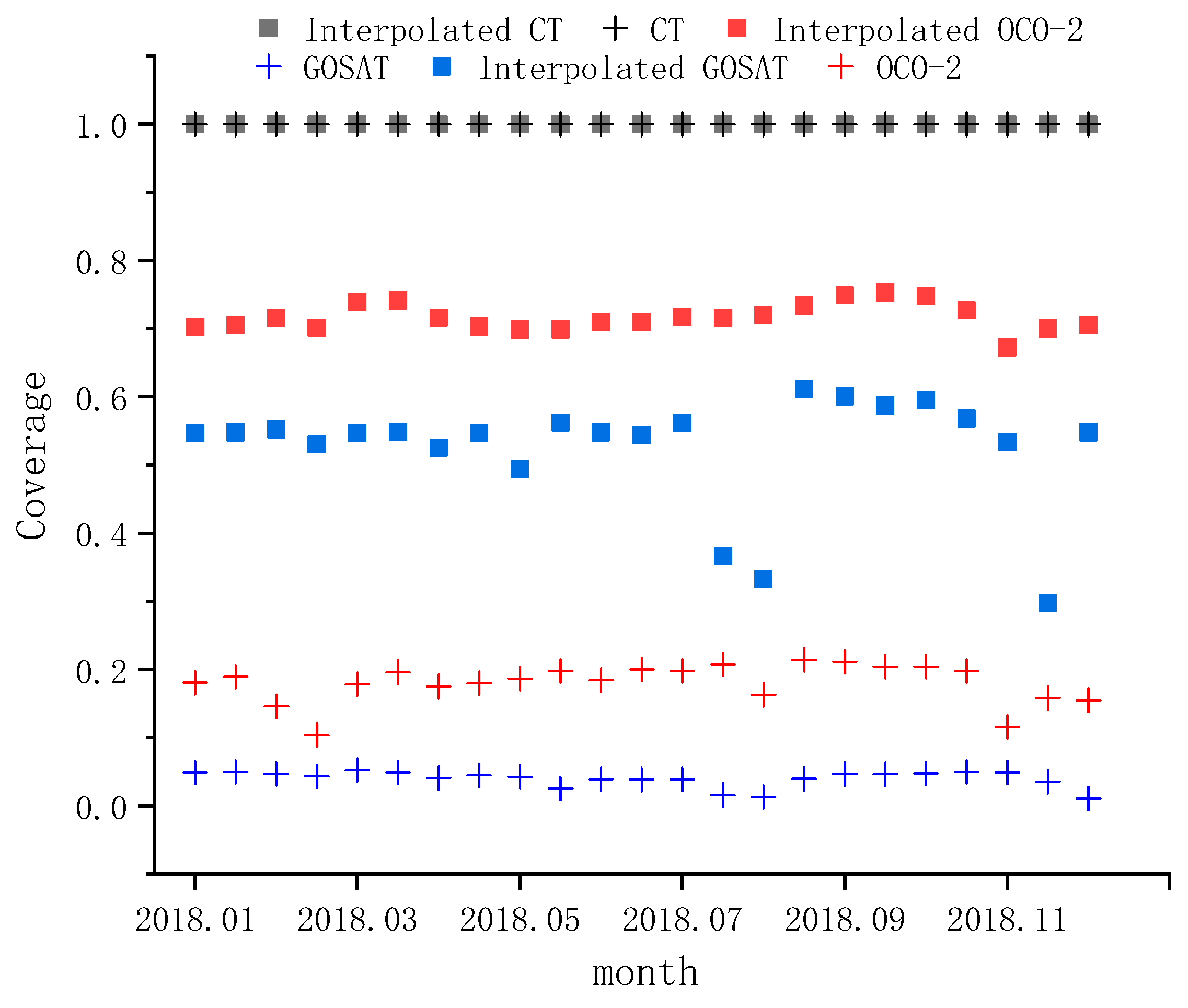
Firstly, we resampled the XCO₂ data of the OCO-2, GOSAT, and CT models to obtain 1° × 1° half-monthly and monthly global XCO₂ datasets. In order to understand the effect of the Kriging model used for interpolating XCO₂ in this paper in more detail, we spatially display the data coverage of OCO-2 and GOSAT datasets before and after Kriging interpolation in Figure 1. At each 1° × 1° grid, if it contains an XCO₂ observation meeting the quality requirements, it is filled with a color (the data before interpolation is dark blue, while the data after interpolation is light blue). The results show that the coverage changes of half-monthly and monthly XCO₂ datasets are basically the same before and after interpolation. The coverage of half-monthly XCO₂ products in 2018 before and after interpolation is shown in Figure 2. In July, August, and December 2018, the coverage of GOSAT data after interpolation does not increase much, because the coverage of GOSAT raw data in these months is low. Overall, before interpolation, the average coverages of OCO-2, GOSAT, and CT products are 18.01%, 3.95%, and 100%, respectively. After interpolation, the average coverages of the OCO-2 and GOSAT datasets are 71.66% and 52.45%, increased by 53.65% and 48.5%, respectively. It can be seen that this method can effectively improve the temporal and spatial resolution of XCO₂ products. We believe that the interpolation results of OCO-2 and GOSAT XCO₂ are mainly affected by the spatial distribution, total number, and sampling interval distribution of observation points. If there is XCO₂ observation in each 1° × 1° grid, or it is evenly distributed in space, this method can obtain XCO₂ data through wider coverage. The coverage of CT reaches 100%, which is due to the time resolution of CT model data being 1 day and the spatial resolution being 3° × 2°; the coverage range is −180°~180° longitude and −90°~90° latitude, and the distribution is uniform. According to the search range of Kriging interpolation, there are data affecting the points to be interpolated. This also paves the way for creating a global seamless 1° × 1° for the later generation XCO₂ dataset, as shown below.

4.2. Fusion of XCO₂ Datasets Based on the TC Algorithm

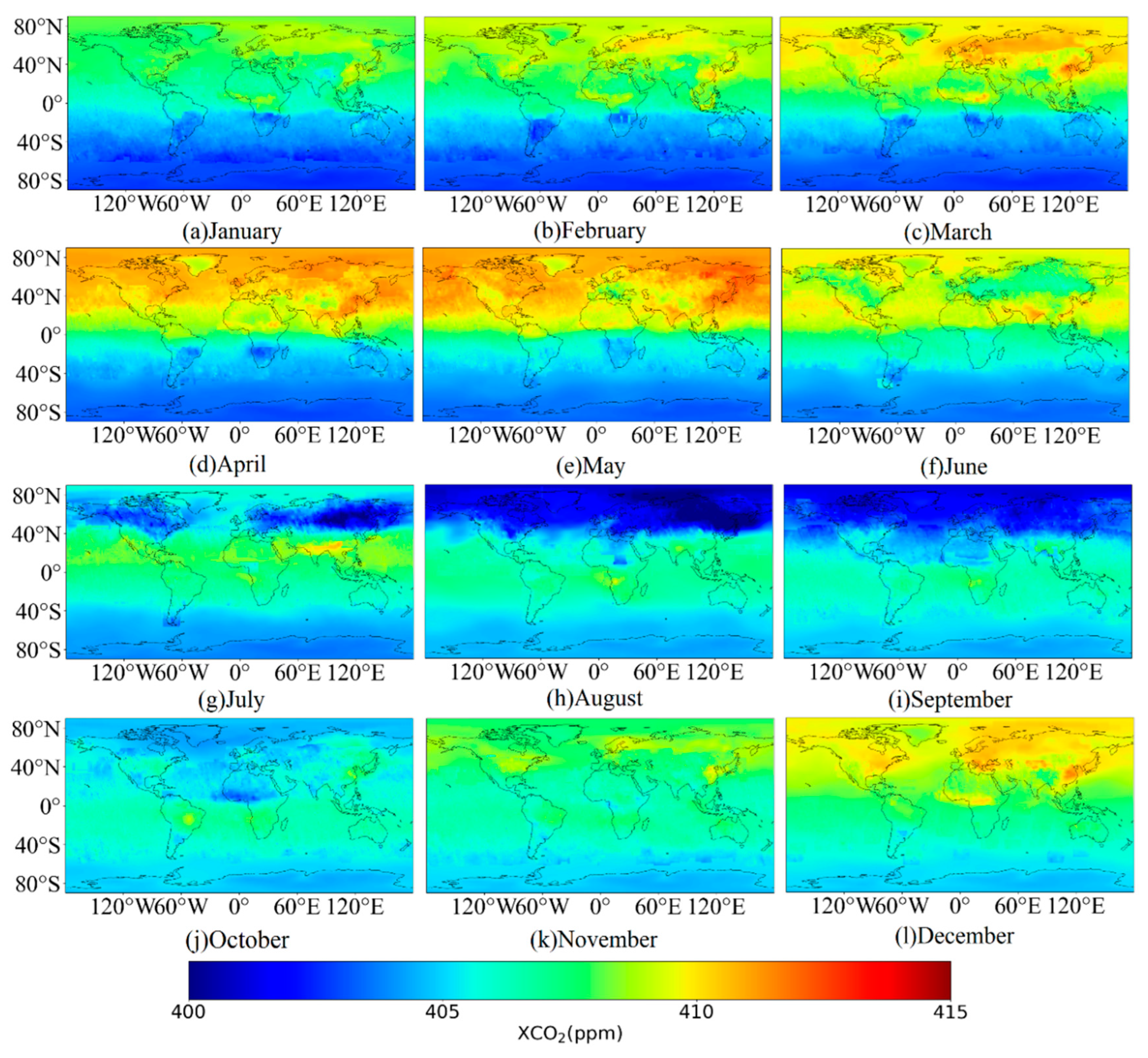
Due to the errors from the satellite inversion algorithm, the limitations of the Earth’s surface and atmospheric conditions, the CO₂ concentrations obtained by satellite have a certain deviation. The CT model obtains the CO₂ concentrations through the data assimilation method, which leads to its excessive dependence on the surface observation data. The CO₂ concentrations obtained in high latitudes and other areas where it is difficult to obtain the observation data have larger deviations, so there are certain random errors in the CO₂ concentrations observed by the satellite and assimilation model. In this study, the TC algorithm was used to evaluate the uncertainty of three XCO₂ products of interpolated OCO-2, GOSAT, and CT. In order to reveal the influence of the time length of the input dataset on obtaining the random error, this study compared the random errors obtained from three different time series of one year, two years, and one month. As shown in

Table 4. Random errors of OCO-2, GOSAT, and CT model.

Time	OCO-2/ppm	GOSAT/ppm	CT/ppm
2017–2018	0.6346	0.7995	0.5273
2018	0.6410	0.8211	0.5196
2018.1	0.5815	0.6991	0.4636

, the differences in random errors between the two-year time series of OCO-2, CT, and GOSAT and the one-year time series are 0.0082, 0.0081, and 0.0349, while the differences in random errors between the two-year time series and the one-month time series are 0.0646, 0.0632, and 0.1505. It shows that the length of the time series has an important impact on the stability of the TC algorithm. When the time series of input data is short, the robustness of the TC algorithm is poor. In this study, the data from 2017 to 2018 were selected as the input dataset. The random errors obtained are CT of 0.5273 ppm, OCO-2 of 0.6346 ppm, and GOSAT of 0.7995 ppm from small to large. The traditional arithmetic average method cannot minimize the random error of the combined results, and the equal weighting coefficient will lead to the introduction of large random errors from GOSAT data, which are particularly obvious in high latitudes. Therefore, the fusion weight should be determined according to the characteristics of the data. Based on the least square principle, combined with the random error based on TC estimation, the weights of the three datasets were calculated by Equation (11). The weights of CT, OCO-2, and GOSAT are 0.4015, 0.3337, and 0.2648, respectively, as shown in

Table 5. Weights of OCO-2, GOSAT, and CT model.

Time	OCO-2	GOSAT	CT
2017–2018	0.3337	0.2648	0.4015
2018	0.3318	0.2590	0.4093
2018.1	0.3241	0.2695	0.4064

. Among them, the CT with the smallest random error has the largest weight, followed by OCO-2 and GOSAT. This means that the XCO₂ dataset generated by fusion depends more on CT data. When a 1° × 1° grid fails to simultaneously have the three XCO₂ data, it is filled with the CT data. Otherwise, it is filled with a new XCO₂ value according to the obtained weights. The results of the TC algorithm fusion in 2018 are shown in Figure 3.

4.3. Accuracy Verification of XCO₂ Fusion Dataset with TCCON Data

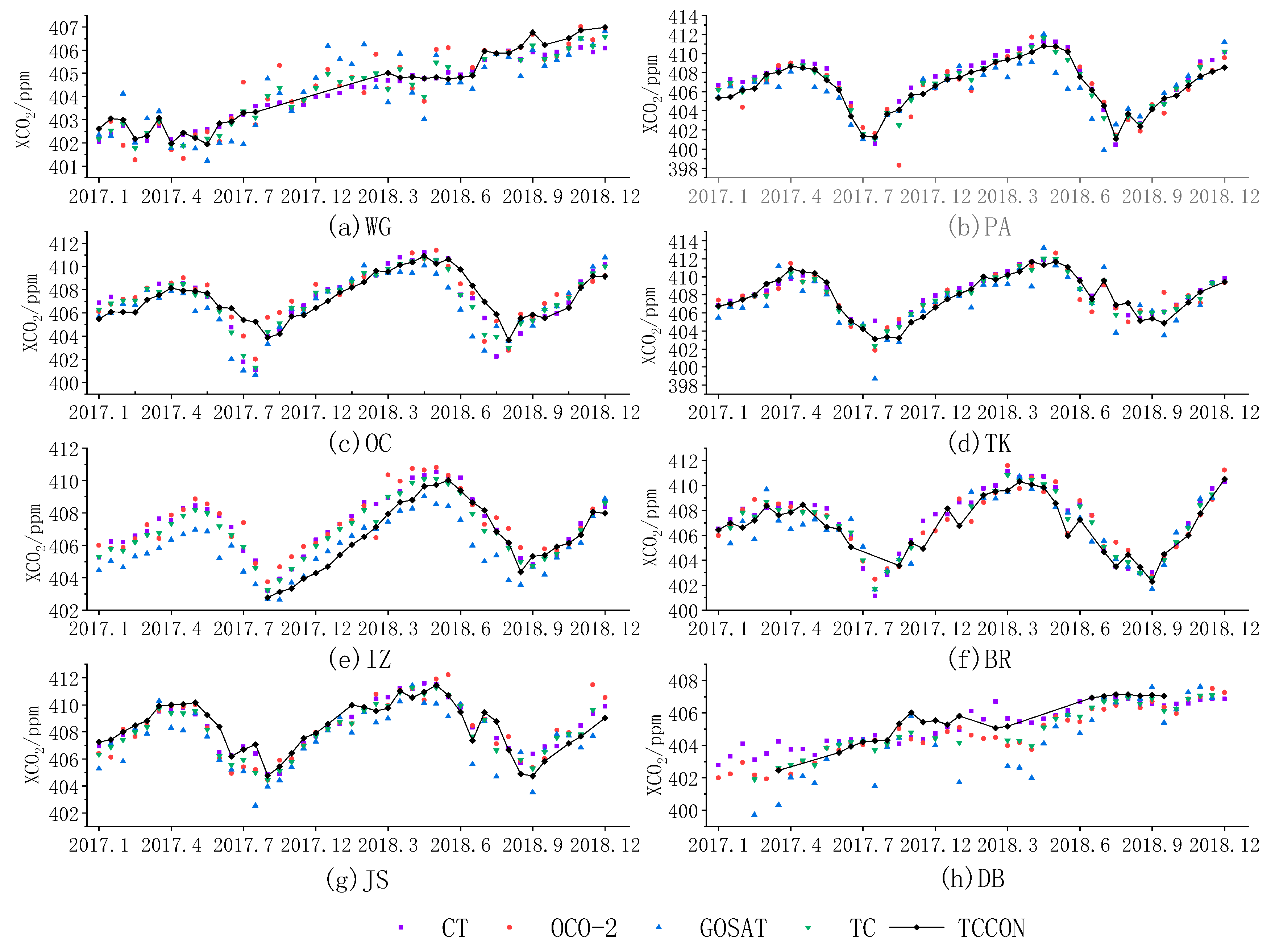
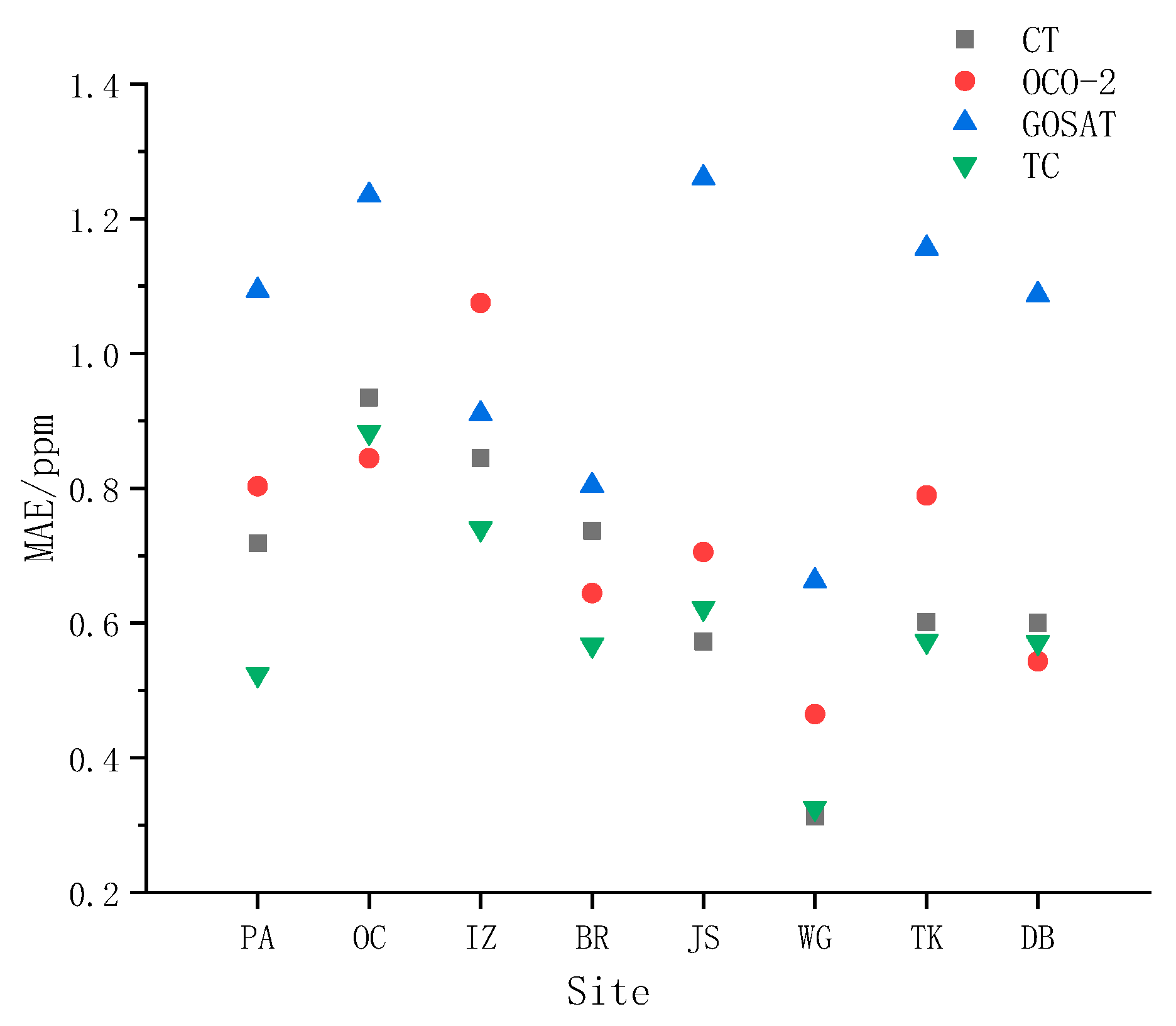
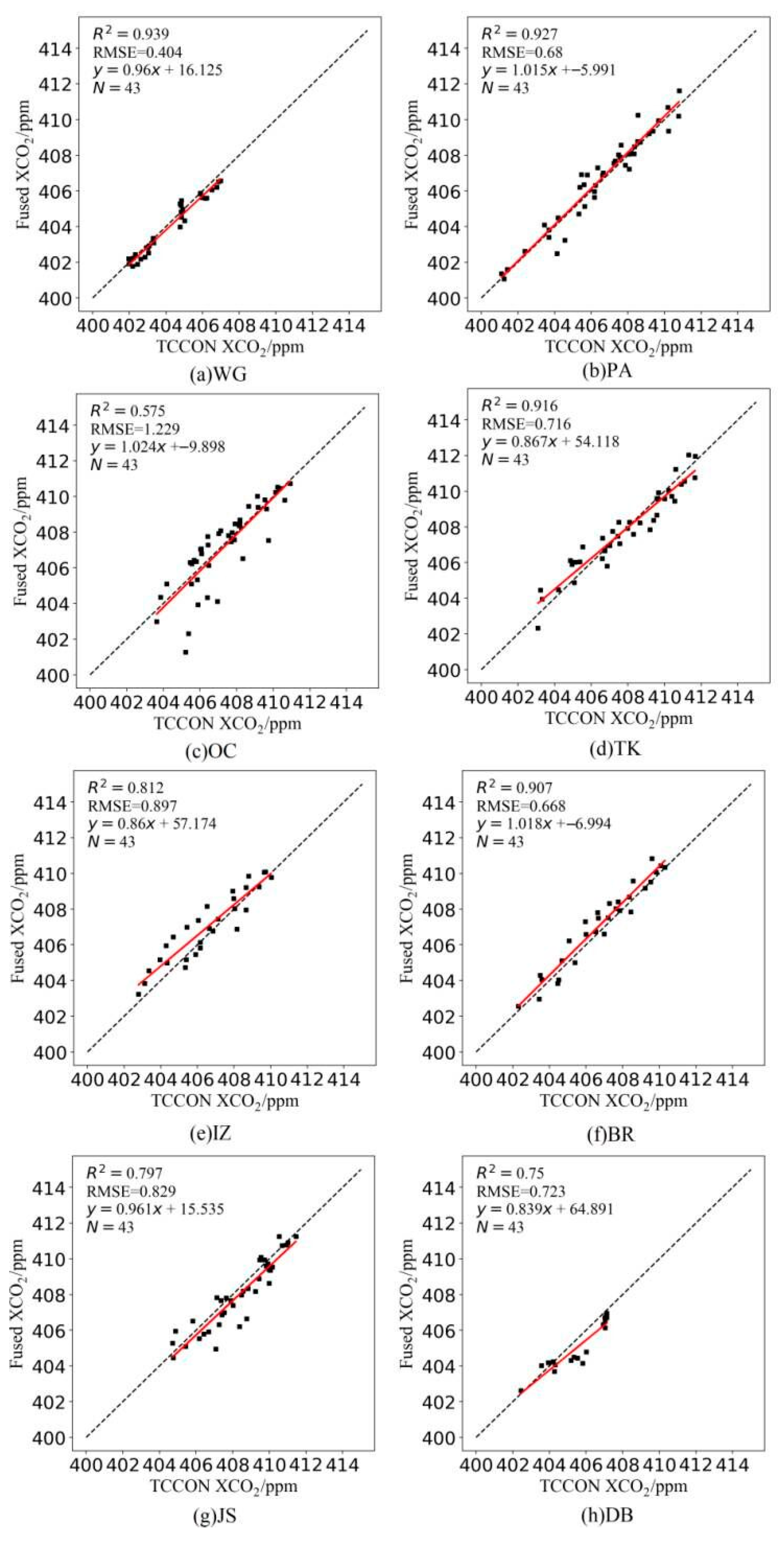
In order to verify the XCO₂ accuracy of the fusion dataset, this study selected the data of eight TCCON sites and compared them with the actual observations of OCO-2, GOSAT, CT and TC fusion data. Figure 4 shows the time series scatter diagram of half-monthly average XCO₂ data from 2017 to 2018 at the eight TCCON sites. At the same time, we calculated the difference between the measured concentrations of TCCON and the four datasets. Figure 5, Figure 6 and Figure 7 show the MAE, RMSE, and R² indicators of the verification results at each TCCON site. In terms of MAE (Figure 5), the average MAE of the TC fusion dataset at the eight sites is 0.6273 ppm, OCO-2 is 0.7628 ppm, GOSAT is 1.0029 ppm, and CT is 0.7306 ppm. In general, the fused XCO₂ values obtained by the TC algorithm are more consistent with that measured by TCCON ground sites. While the average MAE of GOSAT is the largest, which also proves the accuracy of weight allocation to some extent. In terms of RMSE (

Table 6. RMSE of TC Fusion XCO₂, OCO-2 XCO₂, GOSAT XCO₂, and CT XCO₂.

TCCON Site	TC/ppm	OCO-2/ppm	GOSAT/ppm	CT/ppm
PA	0.68	1.235	1.501	0.829
OC	1.229	1.13	1.811	1.312
IZ	0.897	1.278	1.177	1.066
BR	0.668	0.94	1.001	0.963
JS	0.829	0.922	1.556	0.703
WG	0.404	0.631	0.779	0.396
TK	0.716	1.06	1.461	0.784
DB	0.723	0.722	1.56	0.828

), the average RMSE of the TC fusion dataset is 0.7683 ppm, OCO-2 is 0.9898 ppm, GOSAT is 1.3557 ppm, and CT is 0.8601 ppm. At site OC, the RMSEs of the three input datasets are the largest, indicating that there are the largest deviations between the observed values and the measured values at this site, resulting in the high RMSE of the fused dataset. In terms of R² (

Table 7. R² of TC Fusion XCO₂, OCO-2 XCO₂, GOSAT XCO₂, and CT XCO₂.

TCCON Site	TC	OCO-2	GOSAT	CT
PA	0.927	0.8228	0.647	0.8901
OC	0.575	0.7062	0.4657	0.5155
IZ	0.812	0.5826	0.5951	0.7347
BR	0.907	0.8267	0.815	0.8006
JS	0.797	0.8011	0.4588	0.8505
WG	0.939	0.8814	0.7823	0.9414
TK	0.916	0.7852	0.7225	0.896
DB	0.750	0.6201	0.4083	0.6211

and Figure 6), the R² values of the XCO₂ fusion dataset are mostly greater than those of the three input datasets. The average R² of the TC fusion dataset at the eight sites is 0.8279, OCO-2 is 0.7533, GOSAT is 0.6118, and CT is 0.7812. At site OC, the R² of the TC fusion dataset is the smallest because it is affected by the accuracy of CT and GOSAT XCO₂ data. In addition, except for the sites JS and OC, the R² of the TC fusion dataset in all datasets is the highest, and it reaches more than 0.9 at sites PA, Br, WG, and TK. At sites JS and OC, the R² of the fusion dataset is slightly smaller than that of the CT and OCO-2. It shows that the fitting degree between the XCO₂ fusion dataset based on the TC algorithm and the observations of TCCON is good, which proves the feasibility of this method.

4.4. Comparison between Multi-Instrument Fused XCO₂ and TC Fusion Dataset

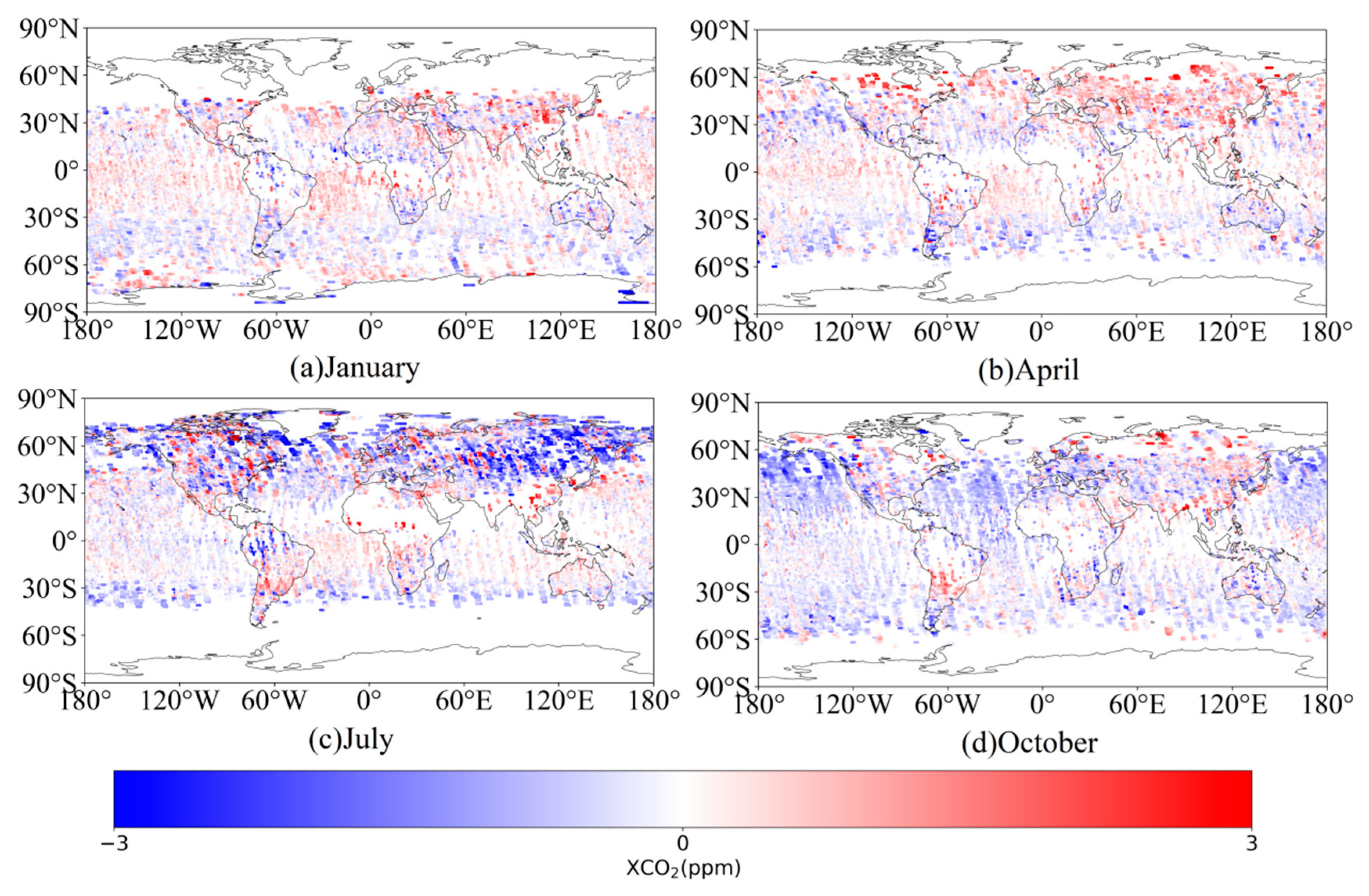
Multi-instrument fused XCO₂ is derived from the Kriging interpolation fusion of OCO-2 and GOSAT Level 2 products, which take a similar approach as the 10-s average using a variation of Kriging. In order to understand the effect of the TC algorithm in fusing XCO₂ in more detail, this paper compared the difference between multi-instrument fused XCO₂ products and XCO₂ obtained by the TC algorithm, and created a quantitative description. In order to show the differences between the two XCO₂ datasets in different regions, Figure 7 displays positive in red and negative in blue, which can intuitively compare the changes in XCO₂ differences under different seasonal conditions. By comparing the MAE and RMSE between January, April, July, and October 2018 on a 15-day scale (

Table 8. Comparison between Fusion Dataset and Multi-instrument Fused XCO₂ MAE and RMSE.

	January	April	July	October
MAE/ppm	0.4803	0.5099	0.8143	0.5486
RMSE/ppm	0.6736	0.7012	1.1405	0.7395

), it is found that there is a small difference in January, April, and October, with an RMSE of 0.6736 ppm, 0.7012 ppm, and 0.7395 ppm, respectively, while there is a large difference in July, with an RMSE of 1.1405 ppm. MAE also shows the same characteristics, with a maximum MAE of 0.8143 ppm in July. This feature is particularly obvious in Asia and Europe, and compared with the multi-instrument fused XCO₂ dataset, the XCO₂ obtained by the TC fusion in this paper is higher, which is more obvious in October. In the marine area, there is little difference. Overall, the products obtained in this paper are in good agreement with multi-instrument fused XCO₂. In January, April, July, and October, there are more than 99.41%, 98.34%, 90.97%, and 98.07% areas with differences within ±2 ppm.

5. Conclusions

OCO-2 and GOSAT satellites are easily restricted by observation conditions, such as aerosols and clouds, resulting in limited coverage of their effective measurements. In order to form XCO₂ data with global coverage, Kriging interpolation was used to improve the coverage and spatial-temporal resolution of OCO-2 and GOSAT data, and CT model data was used as a supplement in this paper. After interpolation, the average coverages of the OCO-2, GOSAT, and CT datasets are 71.66%, 52.45%, and 100%, respectively, and the coverages of OCO-2 and GOSAT are increased by 53.65% and 48.5%, respectively. Furthermore, this paper used the TC algorithm to fuse the CT model dataset with two satellite-interpolated datasets. This algorithm can analyze the uncertainty of datasets by comparing the random errors of three independent datasets, and then determine the weights of three datasets according to the random errors to carry out data fusion. Through cross-validation with TCCON data, the MAE of the fused dataset was 0.6273 ppm, RMSE was 0.7683 ppm, and R² was 0.8279. The results indicate that this method can significantly improve the coverage and accuracy of the XCO₂ dataset.

In this paper, we have obtained the semi-monthly 1° × 1° half-monthly average XCO₂ dataset with good accuracy. Due to the coverage of the original satellite observation data, we cannot further temporarily improve the spatial resolution. However, we still hope to further improve the spatiotemporal resolution of the data to better support future carbon neutrality research. With the continuous development of satellite remote sensing technology, more and more carbon observation satellites have been launched or are planned to be launched. For example, China has launched the world’s first active lidar CO₂ detection satellite—DQ1. Compared with passive remote sensing, active lidar observation has the advantage of all-time and all-weather observation, and can detect global CO₂ concentration with higher resolution and greater coverage [47,48]. At the same time, in order to realize the quantitative monitoring of man-made carbon emissions, which is the core goal of the future carbon satellite observation plan, future carbon monitoring will develop a multi-directional satellite network observation of greenhouse gas concentration, air pollution components, and biomass combustion emissions, as well as a global carbon monitoring constellation with active and passive joints [49]. Therefore, in subsequent studies, multi-source greenhouse gas satellite data and carbon assimilation systems can be combined for interpolation and fusion. In addition, with the increasing number of ground-based observation data, we will consider taking the ground-based observation data as the optimal control condition, multi-satellite interpolation results and carbon assimilation data as the input data, and obtain the XCO₂ fused dataset with a higher spatial-temporal resolution, higher accuracy, and larger coverage based on the TC algorithm, so as to promote the estimation of CO₂ emissions from regional sources and contribute to the research of carbon neutralization.

References

1. Yoshida, Y.; Kikuchi, N.; Morino, I.; Uchino, O.; Yokota, T. Improvement of the retrieval algorithm for GOSAT SWIR XCO2 and XCH4 and their validation using TCCON data. Atmos. Meas. Tech. 2013, 6, 1533–1547. [Google Scholar] [CrossRef]
2. Petit, J.-R.; Raynaud, D. Forty Years of Ice-Core Records of CO2; Nature Publishing Group: London, UK, 2020. [Google Scholar]
3. Zhou, B. Global warming: Scientific progress from AR5 to AR6. Trans. Atmos. Sci. 2021, 44, 667–671. [Google Scholar]
4. Climate Change Center of China Meteorological Administration. Blue Book on Climate Change in China 2020; Science Press: Beijing, China, 2020. [Google Scholar]
5. Chevallier, F.; Engelen, R.J.; Peylin, P. The contribution of AIRS data to the estimation of CO2 sources and sinks. Geophys. Res. Lett. 2005, 32, GL024229. [Google Scholar] [CrossRef]
6. Basu, S.; Guerlet, S.; Butz, A.; Houweling, S.; Hasekamp, O.; Aben, I.; Krummel, P.; Steele, P.; Langenfelds, R.; Torn, M. Global CO2 fluxes estimated from GOSAT retrievals of total column CO2. Atmos. Chem. Phys. 2013, 13, 8695–8717. [Google Scholar] [CrossRef]
7. Saeki, T.; Maksyutov, S.; Saito, M.; Valsala, V.; Oda, T.; RJ, A.; Belikov, D.; Tans, P.; Dlugokencky, E.; Yoshida, Y. Inverse modeling of CO2 fluxes using GOSAT data and multi-year ground-based observations. Sola 2013, 9, 45–50. [Google Scholar] [CrossRef]
8. Bergamaschi, P.; Frankenberg, C.; Meirink, J.F.; Krol, M.; Villani, M.G.; Houweling, S.; Dentener, F.; Dlugokencky, E.J.; Miller, J.B.; Gatti, L.V.; et al. Inverse modeling of global and regional CH4 emissions using SCIAMACHY satellite retrievals. J. Geophys. Res. Atmos. 2009, 114, 45–50. [Google Scholar] [CrossRef]
9. Chen, J.M.; Mo, G.; Deng, F. A joint global carbon inversion system using both CO2 and 13CO2 atmospheric concentration data. Geosci. Model Dev. 2017, 10, 1131–1156. [Google Scholar] [CrossRef]
10. Takagi, H.; Saeki, T.; Oda, T.; Saito, M.; Valsala, V.; Belikov, D.; Saito, R.; Yoshida, Y.; Morino, I.; Uchino, O. On the benefit of GOSAT observations to the estimation of regional CO2 fluxes. Sola 2011, 7, 161–164. [Google Scholar] [CrossRef]
11. Wunch, D.; Toon, G.C.; Wennberg, P.O.; Wofsy, S.C.; Stephens, B.B. Calibration of the Total Carbon Column Observing Network using aircraft profile data. Atmos. Meas. Tech. 2010, 3, 1351–1362. [Google Scholar] [CrossRef]
12. Solomon, S.; Qin, D.; Manning, M.; Chen, Z.; Marquis, M.; Averyt, K.; Tignor, M.; Miller, H. IPCC fourth assessment report (AR4). Clim. Chang. 2007, 374, 1–10. [Google Scholar]
13. Pei, Z.; Han, G.; Shi, T.; Ma, X.; Gong, W. A XCO2 Retrieval Algorithm Coupled Spatial Correlation for the Aerosol and Carbon Detection Lidar. Atmos. Environ. 2023, 309, 119933. [Google Scholar] [CrossRef]
14. Pei, Z.; Han, G.; Mao, H.; Chen, C.; Shi, T.; Yang, K.; Ma, X.; Gong, W. Improving quantification of methane point source emissions from imaging spectroscopy. Remote Sens. Environ. 2023, 295, 113652. [Google Scholar] [CrossRef]
15. Nassar, R.; Jones, D.; Kulawik, S.; Worden, J.; Bowman, K.; Andres, R.J.; Suntharalingam, P.; Chen, J.; Brenninkmeijer, C.; Schuck, T.; et al. Inverse modeling of CO2 sources and sinks using satellite observations of CO2 from TES and surface flask measurements. Atmos. Chem. Phys. 2011, 11, 6029–6047. [Google Scholar] [CrossRef]
16. Yang, D.; Boesch, H.; Liu, Y.; Somkuti, P.; Cai, Z.; Chen, X.; Di Noia, A.; Lin, C.; Lu, N.; Lyu, D.; et al. Toward High Precision XCO2 Retrievals From TanSat Observations: Retrieval Improvement and Validation against TCCON Measurements. J. Geophys. Res. Atmos. 2020, 125, e2020JD032794. [Google Scholar] [CrossRef] [PubMed]
17. Hanhan, Y.; Xianhua, W.; Shichao, W.; Chao, L.; Zhiwei, L.; Hailiang, S.; Wei, X. Atmospheric CO2 retrieval method for satellite observations of greenhouse gases monitoring instrument on GF-5. J. Atmos. Environ. Opt. 2021, 16, 231. [Google Scholar]
18. Katzfuss, M.; Cressie, N. Bayesian hierarchical spatio-temporal smoothing for very large datasets. Environmetrics 2012, 23, 94–107. [Google Scholar] [CrossRef]
19. Reuter, M.; Bösch, H.; Bovensmann, H.; Bril, A.; Buchwitz, M.; Butz, A.; Burrows, J.; O’Dell, C.; Guerlet, S.; Hasekamp, O. A joint effort to deliver satellite retrieved atmospheric CO2 concentrations for surface flux inversions: The ensemble median algorithm EMMA. Atmos. Chem. Phys. 2013, 13, 1771–1780. [Google Scholar] [CrossRef]
20. Nguyen, H.M.; Katzfuss, M.; Cressie, N.; Braverman, A. Spatio-Temporal Data Fusion for Very Large Remote Sensing Datasets. Technometrics 2014, 56, 174–185. [Google Scholar] [CrossRef]
21. Zhang, L.L.; Yue, T.X.; Wilson, J.P.; Zhao, N.; Zhao, Y.P.; Du, Z.P.; Liu, Y. A comparison of satellite observations with the XCO2 surface obtained by fusing TCCON measurements and GEOS-Chem model outputs. Sci. Total Environ. 2017, 601–602, 1575–1590. [Google Scholar] [CrossRef]
22. David, L.; Breon, F.M.; Chevallier, F. XCO2 estimates from the OCO-2 measurements using a neural network approach. Atmos. Meas. Tech. 2021, 14, 117–132. [Google Scholar] [CrossRef]
23. Nol, S.; Reuter, M.; Buchwitz, M.; Borchardt, J.; Warneke, T. XCO2 retrieval for GOSAT and GOSAT-2 based on the FOCAL algorithm. Atmos. Meas. Tech. 2020, 145, 3837–3869. [Google Scholar]
24. Stoffelen, A. Toward the true near-surface wind speed: Error modeling and calibration using triple collocation. J. Geophys. Res. Oceans 1998, 103, 7755–7766. [Google Scholar] [CrossRef]
25. Crisp, D.; Atlas, R.M.; Breon, F.M.; Brown, L.R.; Burrows, J.P.; Ciais, P.; Connor, B.J.; Doney, S.C.; Fung, I.Y.; Jacob, D.J. The Orbiting Carbon Observatory (OCO) mission. Adv. Space Res. 2004, 34, 700–709. [Google Scholar] [CrossRef]
26. Kataoka, F.; Knuteson, R.O.; Kuze, A.; Shiomi, K.; Suto, H.; Yoshida, J.; Kondoh, S.; Saitoh, N. Calibration, Level 1 Processing, and Radiometric Validation for TANSO-FTS TIR on GOSAT. IEEE Trans. Geosci. Remote Sens. 2019, 57, 3490–3500. [Google Scholar] [CrossRef]
27. Peters, W.; Jacobson, A.R.; Sweeney, C.; Andrews, A.E.; Conway, T.J.; Masarie, K.; Miller, J.B.; Bruhwiler, L.M.P.; Pétron, G.; Hirsch, A.I.; et al. An atmospheric perspective on North American carbon dioxide exchange: CarbonTracker. Proc. Natl. Acad. Sci. USA 2007, 104, 18925–18930. [Google Scholar] [CrossRef]
28. Buschmann, M.; Deutscher, N.M.; Sherlock, V.; Palm, M.; Warneke, T.; Notholt, J. Retrieval of xCO(2) from ground-based mid-infrared (NDACC) solar absorption spectra and comparison to TCCON. Atmos. Meas. Tech. 2016, 9, 577–585. [Google Scholar] [CrossRef]
29. Wunch, D.; Toon, G.C.; Blavier, J.-F.L.; Washenfelder, R.A.; Notholt, J.; Connor, B.J.; Griffith, D.W.T.; Sherlock, V.; Wennberg, P.O. The Total Carbon Column Observing Network. Philos. Trans. R. Soc. A Math. Phys. Eng. Sci. 2011, 369, 2087–2112. [Google Scholar] [CrossRef]
30. Ailin, L.; Wei, G.; Ge, H.; Chengzhi, X. Comparison of Satellite-Observed XCO2 from GOSAT, OCO-2, and Ground-Based TCCON. Remote Sens. 2017, 9, 1033. [Google Scholar]
31. Zhang, S.; Bai, Y.; He, X.; Huang, H.; Zhu, Q.; Gong, F. Comparisons of OCO-2 satellite derived XCO2 with in situ and modeled data over global ocean. Acta Oceanol. Sin. 2021, 40, 136–142. [Google Scholar] [CrossRef]
32. Wunch, D.; Wennberg, P.O.; Osterman, G.; Fisher, B.; Naylor, B.; Roehl, C.M.; O’Dell, C.; Mandrake, L.; Viatte, C.; Kiel, M. Comparisons of the orbiting carbon observatory-2 (OCO-2) XCO2 measurements with TCCON. Atmos. Meas. Tech. 2017, 10, 2209–2238. [Google Scholar] [CrossRef]
33. Kulawik, S.; Wunch, D.; O′Dell, C.; Frankenberg, C.; Reuter, M.; Oda, T.; Chevallier, F.; Sherlock, V.; Buchwitz, M.; Osterman, G.; et al. Consistent evaluation of ACOS-GOSAT, BESD-SCIAMACHY, CarbonTracker, and MACC through comparisons to TCCON. Atmos. Meas. Tech. 2016, 8, 6217–6277. [Google Scholar]
34. Buchwitz, M.; Reuter, M.; Schneising, O.; Hewson, W.; Detmers, R.G.; Boesch, H.; Hasekamp, O.P.; Aben, I.; Bovensmann, H.; Burrows, J.P. Global satellite observations of column-averaged carbon dioxide and methane: The GHG-CCI XCO2 and XCH4 CRDP3 data set. Remote Sens. Environ. 2017, 203, 276–295. [Google Scholar] [CrossRef]
35. Zhou, M.; Dils, B.; Wang, P.; Detmers, R.; Mazière, M.D. Validation of TANSO-FTS/GOSAT XCO2 and XCH4 glint mode retrievals using TCCON data from near-ocean sites. Atmos. Meas. Tech. 2015, 8, 10897–10935. [Google Scholar]
36. Kawakami, S.; Ohyama, H.; Arai, K.; Okumura, H.; Taura, C.; Fukamachi, T.; Sakashita, M. TCCON Data from Saga (JP); Release GGG2014. R0 (Version GGG2014. R0); Caltech-DATA: Pasadena, CA, USA, 2022. [Google Scholar]
37. Morino, I.; Matsuzaki, T.; Horikawa, M. TCCON Data from Tsukuba (JP), 125HR; Release GGG2014. R2; CaltechDATA: Pasadena CA, USA, 2018. [Google Scholar]
38. De Mazière, M.; Sha, M.; Desmet, F.; Hermans, C.; Scolas, F.; Kumps, N.; Metzger, J.; Duflot, V.; Cammas, J. TCCON Data from Réunion Island (RE); Release GGG2014. R1 (Version R1); CaltechDATA: Pasadena, CA, USA, 2014. [Google Scholar]
39. Wennberg, P.; Wunch, D.; Roehl, C.; Blavier, J.; Toon, G.; Allen, N.; Dowell, P.; Teske, K.; Martin, C.; Martin, J. TCCON Data from Lamont (US); Release GGG2014. R1; CaltechDATA: Pasadena, CA, USA, 2016. [Google Scholar]
40. Blumenstock, T.; Hase, F.; Schneider, M.; García, O.; Sepúlveda, E. TCCON Data from Izana (ES); Release GGG2014. R1 (Version R1); CaltechDATA: Pasadena, CA, USA, 2017. [Google Scholar]
41. Notholt, J.; Petri, C.; Warneke, T.; Deutscher, N.; Buschmann, M.; Weinzierl, C.; Macatangay, R.; Grupe, P. TCCON Data from Bremen, Germany; Release GGG2014R0; Carbon Dioxide Information Analysis Center, Oak Ridge National Laboratory: Oak Ridge, TN, USA, 2014. [Google Scholar] [CrossRef]
42. Griffith, D.; Velazco, V.; Deutscher, N.; Paton-Walsh, C.; Jones, N.; Wilson, S.; Macatangay, R.; Kettlewell, G.; Buchholz, R.; Riggenbach, M. TCCON Data from Wollongong (AU); Release GGG2014. R0; CaltechDATA: Pasadena, CA, USA, 2014. [Google Scholar]
43. Griffith, D.; Deutscher, N.; Velazco, V.; Wennberg, P.; Yavin, Y.; Keppel-Aleks, G.; Washenfelder, R.; Toon, G.; Blavier, J.; Paton-Walsh, C. TCCON Data from Darwin (AU); Release GGG2014. R0 (Version GGG2014. R0); CaltechDATA: Pasadena, CA, USA, 2014. [Google Scholar]
44. Nalder, I.A.; Wein, R.W. Spatial interpolation of climatic Normals: Test of a new method in the Canadian boreal forest—ScienceDirect. Agric. For. Meteorol. 1998, 92, 211–225. [Google Scholar] [CrossRef]
45. Sreenath, K.R. Introduction to geostatistics. In Winter School on Structure and Function of the Marine Ecosystem; Central Marine Fisheries Research Institute: Kochi, India, 2017. [Google Scholar]
46. Chen, C.; He, M.; Chen, Q.; Zhang, J.; Li, Z.; Wang, Z.; Duan, Z. Triple collocation-based error estimation and data fusion of global gridded precipitation products over the Yangtze River basin. J. Hydrol. 2021, 605, 127307. [Google Scholar] [CrossRef]
47. Shi, T.; Han, G.; Ma, X.; Pei, Z.; Chen, W.; Liu, J.; Zhang, X.; Li, S.; Gong, W. Quantifying strong point sources emissions of CO2 using spaceborne LiDAR: Method development and potential analysis. Energy Convers. Manag. 2023, 292, 117346. [Google Scholar] [CrossRef]
48. Shi, T.; Han, G.; Ma, X.; Mao, H.; Chen, C.; Han, Z.; Pei, Z.; Zhang, H.; Li, S.; Gong, W. Quantifying factory-scale CO2/CH4 emission based on mobile measurements and EMISSION-PARTITION model: Cases in China. Environ. Res. Lett. 2023, 18, 034028. [Google Scholar] [CrossRef]
49. Liu, L.; Chen, L.; Liu, Y.; Yang, D.; Zhang, X.; Lu, N.; Ju, W.; Jiang, F.; Yin, Z.; Liu, G. Satellite remote sensing for global stocktaking: Methods, progress and perspectives. Natl. Remote Sens. Bull. 2022, 26, 243–267. [Google Scholar] [CrossRef]
Figure 1. Distribution of coverage of OCO-2 and GOSAT XCO2 for the first half of the month (left graphs) and a full month (right graphs) in January 2018. The satellite observation data are displayed in dark blue, and the interpolated data are displayed in light blue.
Atmosphere 14 01335 g001aAtmosphere 14 01335 g001b
Figure 2. Half-monthly XCO2 data coverage before and after interpolation of OCO-2, GOSAT, and CT in 2018.
Atmosphere 14 01335 g002
Figure 3. XCO2 distribution of fusion dataset in 2018.
Atmosphere 14 01335 g003
Figure 4. Scatter diagrams of time series of OCO-2, GOSAT, CT, and TC fusion XCO2 data at the eight TCCON sites from 2017 to 2018. The black solid line represents the observations of the TCCON site, the purple point represents CT, the red point represents OCO-2, the blue point represents GOSAT, and the green point represents the fused XCO2 based on the TC algorithm.
Atmosphere 14 01335 g004
Figure 5. MAE of TC fusion XCO2, OCO-2 XCO2, GOSAT XCO2, and CT XCO2.
Atmosphere 14 01335 g005
Figure 6. Correlation analysis between TCCON and fused XCO2 data.
Atmosphere 14 01335 g006
Figure 7. Comparison of difference between fusion products and multi-instrument fused XCO2.
Atmosphere 14 01335 g007