Abstract
As the penetration rate of wind power in the grid continues to increase, wind speed forecasting plays a crucial role in wind power generation systems. Wind speed prediction helps optimize the operation and management of wind power generation, enhancing efficiency and reliability. However, wind speed is a nonlinear and nonstationary system, and traditional statistical methods and classical intelligent algorithms struggle to cope with dynamically updating operating conditions based on sampled data. Therefore, from the perspective of optimizing intelligent algorithms, a wind speed prediction model for wind farms was researched. In this study, we propose the Deterministic Broad Learning System (DBLS) algorithm for wind farm wind speed prediction. It effectively addresses the issues of data saturation and local minima that often occur in continuous-time system modeling. To adapt to the continuous updating of sample data, we improve the sample input of the Broad Learning System (BLS) by using a fixed-width input. When new samples are added, an equivalent number of old samples is removed to maintain the same input width, ensuring the feature capture capability of the model. Additionally, we construct a dataset of wind speed samples from 10 wind farms in Gansu Province, China. Based on this dataset, we conducted comparative experiments between the DBLS and other algorithms such as Random Forest (RF), Support Vector Regression (SVR), Extreme Learning Machines (ELM), and BLS. The comparison analysis of different algorithms was conducted using Root Mean Square Error (RMSE) and Mean Absolute Percentage Error (MAPE). Among them, the DBLS algorithm exhibited the best performance. The RMSE of the DBLS ranged from 0.762 m/s to 0.776 m/s, and the MAPE of the DBLS ranged from 0.138 to 0.149.
1. Introduction
Today, the collection of time series data is widely used in many fields. By processing and analyzing historical time series data, complex system models can be established [1]. These models can predict the development trends of systems and effectively solve problems where the operating mechanisms of complex systems are difficult to analyze [2,3,4]. Based on the nature of time series data, the requirements of the system problem, and the suitability of algorithms, common processing algorithms for time series data include univariate processing algorithms, multivariate processing algorithms [5], flat processing algorithms, linear processing algorithms, nonlinear processing algorithms, and algorithms for handling different time scales [6]. Researchers aim to develop models that accurately predict future values and thus forecast the numerical values, trends, or patterns of future time points or periods based on existing historical data [7,8,9].
Researchers have conducted extensive research on the analysis of complex system problems and the stability and accuracy of time series prediction models. Many well-performing research outcomes have been achieved. Common statistical algorithms include Auto Regression Moving Average (ARMA) [10], Auto Regressive Integrated Moving Average (ARIMA) [11], Seasonal Auto-Regressive Integrated Moving Average (SARIMA) [12], Seasonal Trend Loss (STL) [13], Exponential Smoothing, Linear Regression, and Generalized Auto Regressive Conditional Heteroskedasticity (GARCH) [14]. Common intelligent algorithms include Artificial Neural Networks (ANNs) [15], Long Short-Term Memory (LSTM) [16] and its variants, Convolutional Neural Networks (CNNs) [17,18] and their variants, Support Vector Regression (SVR) [19,20] and its variants, Random Forest [21,22,23], Deep Learning [24,25] and its variants, and Genetic Algorithms [26,27] and their variants. These algorithms represent static nonlinear mapping relationships, and the stability and accuracy of prediction models are affected when sample data are dynamically updated. Additionally, most of these algorithms are based on iterative processes using gradient information, which results in time-consuming model updates and high computational resource utilization when sample data are dynamically updated.
Single-Layer Feedforward Neural Networks (SLFNs) are widely used for time series data modeling due to their simple structure and high computational efficiency [28]. However, SLFNs are sensitive to parameter settings and learning rates. In light of this, some researchers have proposed the Random Vector Functional-Link Neural Network (RVFLNN) [29], which is widely applied in time series modeling analysis and control systems due to its approximation performance and fast learning characteristics. However, the predictive performance and stability of the RVFLNN model are diminished when dealing with high-dimensional and time-varying datasets. Chen C L P and his colleagues proposed the Broad Learning System (BLS) [30,31,32], which is suitable for multidimensional and time-varying datasets. This algorithm enables fast modeling and rapid model updates, making it applicable in various fields. Cheng Y and others proposed the D-BLS algorithm for load trend prediction [33]. Wang M and his team combined adaptive Kalman filtering with the BLS for battery-charging-state detection, achieving excellent detection results [34]. Pu X and his colleagues developed an online semisupervised Broad Learning System and applied it to industrial fault detection, obtaining satisfactory performance [35]. Chu F and his collaborators applied the BLS to nonlinear systems, effectively capturing nonlinear features and system descriptions, thus improving the predictive accuracy and robustness of the model [36]. Additionally, the BLS has also found numerous applications in the energy sector.
Wind condition prediction in wind farms plays a crucial role in optimizing the power output of wind turbines, ensuring the efficient operation of the wind farm, and facilitating the grid integration and scheduling of wind power. Wind conditions in wind farms are influenced by factors such as temperature, pressure, humidity, altitude, season, atmospheric circulation, time, latitude and longitude, and geographical environment. A wind farm is a complex and nonlinear system with multiple couplings, representing a continuous-time series system. Currently, scholars have conducted extensive research to establish accurate and effective wind condition models for wind farms. Chen, CL Philip provided an approximation proof of the BLS in the literature [37] and applied it to wind speed prediction, greatly reducing the training time of samples. Wang S and others combined statistics with the Broad Learning System to effectively predict the formation of offshore storms [38]. Jiao, Xuguo, and their team developed the VMD-BLS wind speed prediction model and improved the model’s prediction accuracy through error compensation [39]. However, when considering the continuous-time updating of sample data, the stability and accuracy of the prediction models for wind farm conditions and power generation have difficulty meeting the desired expectations.
When the sample data are continuously updated, the aforementioned algorithms are prone to data saturation and getting trapped in local minima. In most cases, the stability and accuracy of the prediction models are greatly reduced. It is difficult to achieve reliable predictions under the continuous updating of sample data. In the context of continuous updates to wind farm wind speed, the mentioned algorithms may experience data saturation, leading to a loss of the ability to capture dynamic features within the models. The algorithms mentioned above may encounter data saturation and lose the ability to capture dynamic features when the sample data are continuously updated. In this paper, we propose the DBLS algorithm and apply it to wind speed prediction under continuous operating conditions, resulting in stable and accurate prediction models. To adapt to the continuous updating of sample data, the system input is changed to a fixed-width input. When new samples are added, an equal number of old samples are removed to maintain a constant input width for the system. This approach preserves some of the original features while incorporating new system characteristics through the addition of new samples. We established a sample dataset of wind speed from 10 wind farms in Gansu Province, China, and applied the DBLS algorithm to the constructed dataset. Furthermore, comparative experiments were conducted between the DBLS algorithm and the RF, SVR, ELM, and BLS algorithms. The experimental results demonstrate that the DBLS algorithm exhibits good stability and prediction accuracy.
The main contributions of this research are as follows:
- The primary contribution of this research project is the introduction of the Deterministic Broad Learning System, addressing the issues of data saturation and local minima that commonly occur when the sample data are continuously updated. By adapting the system input to a fixed-width input, the proposed model achieves good prediction accuracy.
- The collection and establishment of a sample dataset of wind speed from 10 wind farms in Gansu Province, China.
- The application of the DBLS algorithm to wind speed prediction in wind farms, with comparative experiments conducted against RF, SVR, ELM, and BLS. The experimental results demonstrate that the DBLS algorithm performs well in terms of stability and prediction accuracy.
2. BLS
Chen [30] presented the BLS architecture based on RVFLNNs. Unlike deep networks, it does not have multiple layers of deep network superposition, only containing an input layer, feature layer, and output layer. The characteristics of the BLS are as follows:
- (1)
- The input of the BLS is to perform a linear random mapping of samples to form feature nodes, which facilitates the network to be easily integrated with other neural networks when required.
- (2)
- In the output layer, the BLS takes the feature node and the enhancement node together as the input of the output layer. Here, we notice that the feature node is a linear mapping of the input sample, which can effectively reduce the loss of sample features.
The BLS network structure is shown in Figure 1. The input sample X is mapped as a feature node through a linear random link function. The feature nodes as a whole map different enhancement nodes through nonlinear random functions. The middle layer of the BLS is composed of feature nodes and enhancement nodes. The specific operation principle will be analyzed in detail in the following content.
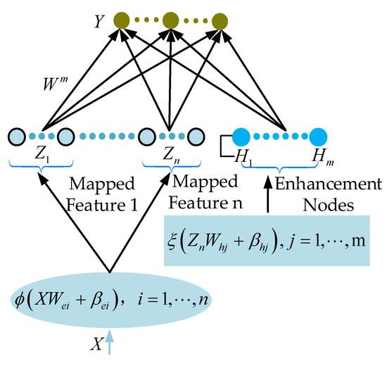
Figure 1.
The structure of BLS [37].
The mathematical theoretical support for the BLS is given in [37]. Therefore, only a brief overview of the principles of the BLS is provided. Feature nodes are calculated using Equation (1) [37].
In Equation (1), is the input sample set. is the ith feature window obtained by solving Formula (1). is the linear mapping function. and are randomly generated weights and offsets, respectively.
The enhancement nodes are obtained via Equation (2) [37], which is a linear function.
where and are randomly generated weights and offsets.
On the basis of Equations (1) and (2), the output layer of the BLS can be expressed via Equation (3) [37].
where . is the output function weight.
3. Incremental Broad Learning System
In order to better apply the BLS network, the continuous updating of network input is studied. Generally, when the input sample is updated, most network structures update the weight and bias via retraining, while the BLS can update the weight and bias without retraining. This feature greatly reduces the training time and provides a good basis for online training.
Let the original input sample dataset be , where is an additional input sample. At this point, the structure of the BLS network is shown in Figure 2. The middle layer of the BLS can be represented as . can be found using Equation (4).
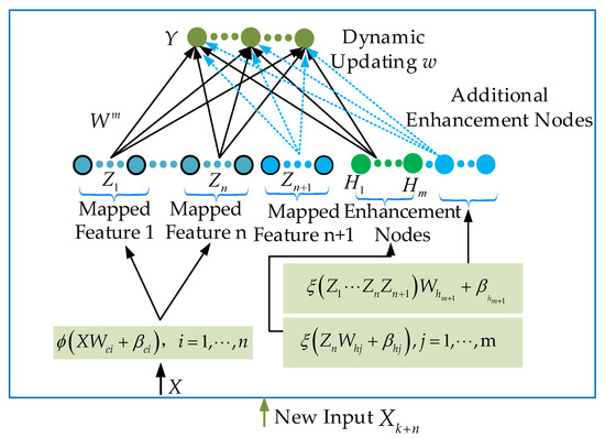
Figure 2.
BLS structure with increasing input samples [37].
In Equation (4), represents the intermediate layer of the BLS at the time of the original sample set input. is the middle layer addition variable corresponding to the added input sample .
The output weights of the BLS network are updated to , which can be obtained by deriving Equation (5).
thus finding
is the label for the new input sample .
Let . Furthermore, it follows that
By deducing from Equation (6), it follows that
4. Deterministic Broad Learning System
From Equations (8) and (9), it can be obtained that data saturation linearity will occur as n tends to infinity. Therefore, when introducing the BLS into dynamic systems, the Deterministic Broad Learning System (DBLS) is proposed to solve the data saturation problem. The structure of the DBLS is shown in Figure 3.
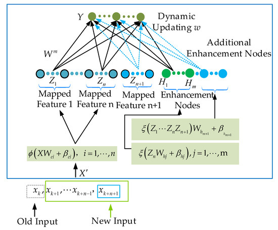
Figure 3.
DBLS structure with input samples.
The DBLS uses a fixed input dimension, i.e., for each new set of data, an old set of data is removed. For example, let the input dimension of F be fixed as n. A new set of data is added, and a set of old data is removed to maintain the fixed dimension. Here, the weight of F can be calculated via Equations (10) and (11).
The DBLS is effective in overcoming data saturation, as demonstrated below. The relevant proof is made using the counterfactual method.
(1) The difference equation for the error vector with respect to the DBLS output weights is constructed.
We perform a difference operation on both ends of Equation (10) with , and we derive
such that
The difference equation for can be derived via
(2) Stability analysis of Equation (14)
Let the eigenvalue of be and the corresponding eigenvector be . We have that
Taking Equation (15) into Equation (13), we have
We further transform Equation (16) to obtain
Since both and are positive definite matrices, it can be deduced from Equation (17) that
We can obtain by solving Equation (18) that or .
Equation (14) is unstable, so we can obtain
Clearly contradicting the previous assumptions, the DBLS does not suffer from data update saturation and is able to converge stably. The DBLS algorithm is presented in Algorithm 1. The DBLS algorithm flowchart is shown in Figure 4.
| Algorithm 1 Deterministic Broad Learning System |
| Input: training sample X; |
| Output: W |
|
| Set |
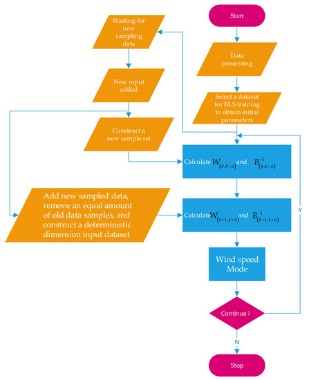
Figure 4.
DBLS algorithm flowchart.
5. Validation and Analysis
The dataset was derived from ten wind farms located in Gansu Province, China. The dataset includes information such as time, wind speed, temperature, air pressure, and humidity at 70 m. It encompasses data from the year 2021. The training and testing sample information used during the experimental analysis is presented in Table 1. Table 1 provides the basic information of the dataset, where the four features related to wind speed are time, temperature, pressure, and humidity. Wind speed is the label in the dataset; therefore, the dataset encompasses a total of five categories, including time, temperature, pressure, humidity, and wind speed.

Table 1.
The dataset information.
Before conducting the experiments, the dataset was preprocessed. The DBLS model was applied to the dataset consisting of 10 wind farms. Additionally, comparative experiments were conducted between the DBLS and other algorithms such as RF, SVR, ELM, and BLS. During the experiments, the parameters of the DBLS model were set as follows:
- The initial values and of the DBLS algorithm were derived offline using batch BLS.
- Number of feature windows (NnmWin): Selected from {5, 6, …, 20}, and in this experiment, NnmWin was set to 7.
- Number of feature nodes (NumFea): Selected from {5, 6, …, 30}, and in this experiment, NumFea was set to 10.
- Number of enhancement nodes (NumEnhan): Selected from {100, 200, …, 1000}, and in this experiment, NumEnhan was set to 300.
- Scaling factor (s) for enhancement nodes: Set to 0.8 in this experiment.
- Regularization parameter (C): Set to 2−30 in this experiment.
The experiment utilized the data from the first 25 days of each month as the training set, while the remaining days of the month were used as the testing set. When using the DBLS for wind speed prediction, the Root Mean Square Error (RMSE) and Mean Absolute Percentage Error (MAPE) are commonly adopted as evaluation metrics for assessing prediction performance. The formulas for calculating RMSE and MAPE are as follows:
where l represents the number of samples, denotes the actual observed values, and represents the predicted values.
While conducting experiments on the wind speed of the established wind farm dataset, the DBLS model was configured with the following parameters: the feature layer window size was set to 7, each window had 10 nodes, the enhancement nodes were set to 300, and the regularization parameter ranged from 2−30. In order to compare the predictive performance of the models, taking the wind speed dataset at 70 m as an example, the DBLS model was compared with the BLS, RF, SVR, and ELM models through experiments. Table 2 presents the parameter settings for the comparative experiments with different models. Figure 5 presents the prediction results of different algorithms.

Table 2.
Parameter settings for different model experiments.
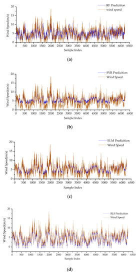
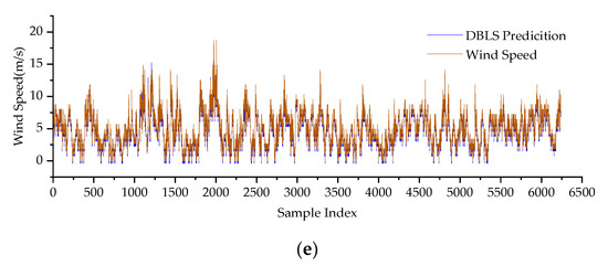
Figure 5.
The prediction results of different algorithms: (a) Comparison graph between the wind speed model at 30 m based on the RF algorithm and the original wind speed. (b) Comparison graph between the wind speed model at 70 m based on the SVR algorithm and the original wind speed. (c) Comparison graph between the wind speed model at 70 m based on the ELM algorithm and the original wind speed. (d) Comparison graph between the wind speed model at 70 m based on the BLS algorithm and the original wind speed. (e) Comparison graph between the wind speed model at 70 m based on the DBLS algorithm and the original wind speed.
In Table 2, the RF model includes the following parameters: estimators represent the number of trees, min_samples_split represents the minimum number of samples required to split a node, and max_depth represents the maximum depth of the trees. In the SVR model, C represents the penalty factor for error terms, and γ represents the coefficient of the kernel function. For the ELM model, C represents the regularization coefficient and Hidden Num represents the number of hidden layers. In the BLS and DBLS models, Num Win represents the number of windows in the feature layer, Num Fea represents the number of nodes in each window, Num Enhan represents the number of enhancement nodes, and C represents the regularization parameter. After setting the parameters, the DBLS model was validated using the aforementioned dataset. The wind speed was used as the target variable in this experiment, and the remaining features were used as input data. The predictive metrics for different models on various datasets are presented in Table 3.

Table 3.
RMSE and MAPE for different models.
Based on the data in Table 3, it can be observed that the DBLS performs better than the other models in predicting wind speed. In the application experiments involving 10 wind farms, a comparison between the DBLS and BLS algorithms reveals a significant improvement in the learning accuracy of the DBLS, validating the findings in Figure 4. Under the condition of continuous system updates and dynamic prediction, the weight values of the BLS algorithm cannot be promptly adjusted, resulting in a weakened ability to capture new features. However, the DBLS algorithm overcomes the issue of data saturation during continuous data updates by employing a fixed-width input and removing an equal amount of old data as new data are added. Therefore, in the context of nonlinear dynamic modeling and when system characteristics change, the weight values of the DBLS can be quickly adjusted to rapidly adapt to the system characteristics, leading to better prediction accuracy.
6. Discussion
This study investigated a predictive model for wind speed in wind farms. Wind speed in wind farms is a complex nonlinear system with multiple coupled parameters. Therefore, establishing a wind speed prediction model using intelligent algorithms has become an important research direction. The challenge of wind speed prediction models lies in whether they can maintain prediction accuracy and generalization stability under dynamically changing operational conditions.
Taking advantage of the online Broad Learning System, the DBLS algorithm is proposed from the perspective of dynamically updating weights. This algorithm addresses the stability issue of prediction accuracy and the generalization characteristics of wind speed prediction models under continuously changing operational conditions. Applying the DBLS algorithm to 10 wind farm datasets, the RMSE errors range from 0.762 m/s to 0.776 m/s, and the MAPE errors range from 0.138 to 0.149. Experimental results indicate high prediction accuracy and strong generalization ability.
A comparative analysis experiment was conducted by comparing the DBLS algorithm with the RF, SVR, ELM, and BLS algorithms. From the experimental results, it can be observed that the DBLS algorithm exhibits more prominent performance. In future research, the DBLS algorithm will be introduced into time series prediction applications under similar operational conditions to expand its application scope. Additionally, further research will delve into optimizing the optimal network structure of the DBLS algorithm to enhance its performance. Wind speeds in wind farms typically constitute complex nonlinear systems with multiple interdependent elements. Wind speeds within wind farms often manifest as nonstationary and nonuniform wind fields. References [40,41,42] thoroughly discuss and analyze nonstationary and nonuniform wind fields, providing directions and insights for our subsequent research. In the upcoming phases of our study, we will delve deeper into these aspects.
7. Conclusions
The working mechanism of an online BLS was analyzed, and based on that, the DBLS algorithm was proposed. The theoretical derivation process and convergence proof of the DBLS algorithm were provided. The DBLS algorithm effectively solves the issue of data saturation that occurs while continuously updating samples in nonlinear system modeling. The initial weight values of the algorithm are obtained through batch sample training. Subsequently, the algorithm uses fixed-width input, which means that when new samples are inputted, an equal amount of old sample data are removed. Therefore, the algorithm can better approximate time-varying nonlinear systems. Additionally, a dataset of 10 wind farms in Gansu Province, China, was established. Finally, a comparative experiment was conducted on the constructed dataset, comparing the performance of the DBLS with the BLS, RF, SVR, and ELM algorithms. The experimental results showed that the approximation performance of the DBLS algorithm was superior to that of other algorithms, further validating the reliability of the corresponding theoretical analysis.
The DBLS performs well in wind speed prediction for wind farms. Additionally, it is noted that the number of nodes in the DBLS network is currently determined through multiple experimental trials to achieve relative optimization. Therefore, how to obtain the optimal network structure for DBLS will be a focal point of future research. Currently, our research team is exploring the application of the DBLS in other temporal domains, and more relevant research outcomes will be provided in the future.
Author Contributions
Conceptualization, L.W. and A.X.; methodology, L.W. and A.X.; software, L.W.; validation, L.W.; formal analysis, L.W.; investigation, L.W. and A.X.; resources, L.W.; data curation, L.W.; writing—original draft preparation, L.W.; writing—review and editing, L.W. and A.X.; supervision, L.W.; project administration, L.W.; funding acquisition, L.W. All authors have read and agreed to the published version of the manuscript.
Funding
This research received no external funding.
Institutional Review Board Statement
Not applicable.
Informed Consent Statement
Not applicable.
Data Availability Statement
The datasets of the current study are available from the corresponding author on reasonable request.
Conflicts of Interest
The authors declare no conflict of interest.
Abbreviations and Symbols
| DBLS | Deterministic Broad Learning System |
| BLS | Broad Learning System |
| RF | Random Forest |
| SVR | Support Vector Regression |
| ELM | Extreme Learning Machines |
| RMSE | Root Mean Square Error |
| MAPE | Mean Absolute Percentage Error |
| ARMA | Auto Regression Moving Average |
| ARIMA | Auto Regressive Integrated Moving Average |
| SARIMA | Seasonal Auto Regressive Integrated Moving Average |
| STL | Seasonal Trend Loss |
| GARCH | Generalized Auto Regressive Conditional Heteroskedasticity |
| ANNs | Artificial Neural Networks |
| LSTM | Long Short-Term Memory |
| CNNs | Convolutional Neural Networks |
| SVR | Support Vector Regression |
| SLFNs | Single-Layer Feedforward Neural Networks |
| RVFLNN | Random Vector Functional Link Neural Network |
| the ith feature window | |
| the linear mapping function | |
| the weights of the function | |
| the biases of the function | |
| the mapping function of the enhancement node | |
| the weights of the function | |
| the biases of the function | |
| the output function weight | |
| X | the input sample |
| the intermediate layer of the BLS | |
| the middle layer addition variable corresponding to the added input sample | |
| the inverse of | |
| the inverse of | |
| the difference equation |
References
- Tao, T.; Shi, P.; Wang, H.; Ai, W. Short-term prediction of downburst winds: A double-step modification enhanced approach. J. Wind Eng. Ind. Aerodyn. 2021, 211, 104561. [Google Scholar] [CrossRef]
- Dolatabadi, A.; Abdeltawab, H.; Mohamed, Y.A.R.I. Deep spatial-temporal 2-D CNN-BLSTM model for ultrashort-term LiDAR-assisted wind turbine’s power and fatigue load forecasting. IEEE Trans. Ind. Inform. 2021, 18, 2342–2353. [Google Scholar] [CrossRef]
- Ran, X.; Xu, C.; Ma, L.; Xue, F. Wind Power Interval Prediction with Adaptive Rolling Error Correction Based on PSR-BLS-QR. Energies 2022, 15, 4137. [Google Scholar] [CrossRef]
- Wang, L.; Wang, Y.; Chen, J.; Shen, X. A PM2.5 Concentration Prediction Model Based on CART–BLS. Atmosphere 2022, 13, 1674. [Google Scholar] [CrossRef]
- Jiang, Y.; Liu, S.; Zhao, N.; Xin, J.; Wu, B. Short-term wind speed prediction using time varying filter-based empirical mode decomposition and group method of data handling-based hybrid model. Energy Convers. Manag. 2020, 220, 113076. [Google Scholar] [CrossRef]
- Han, L.; Li, M.J.; Wang, X.J.; Lu, P.P. Wind power forecast based on broad learning system and simplified long short term memory network. IET Renew. Power Gener. 2022, 16, 3614–3628. [Google Scholar] [CrossRef]
- Li, D.; Chen, D.; Jin, B.; Shi, L.; Goh, J.; Ng, S.K. MAD-GAN: Multivariate anomaly detection for time series data with generative adversarial networks. In Proceedings of the International Conference on Artificial Neural Networks, Munich, Germany, 17–19 September 2019; pp. 703–716. [Google Scholar]
- Kim, H.S.; Han, K.M.; Yu, J.; Kim, J.; Kim, K.; Kim, H. Development of a CNN+LSTM Hybrid Neural Network for Daily PM2.5 Prediction. Atmosphere 2022, 13, 2124. [Google Scholar] [CrossRef]
- Löwe, S.; Madras, D.; Zemel, R.; Welling, M. Amortized causal discovery: Learning to infer causal graphs from time-series data. In Proceedings of the Conference on Causal Learning and Reasoning, Eureka, CA, USA, 11–13 April 2022; pp. 509–525. [Google Scholar]
- Pappas, S.S.; Ekonomou, L.; Karamousantas, D.C.; Chatzarakis, G.E.; Katsikas, S.K.; Liatsis, P. Electricity demand loads modeling using AutoRegressive Moving Average (ARMA) models. Energy 2008, 33, 1353–1360. [Google Scholar] [CrossRef]
- Nelson, B.K. Time series analysis using autoregressive integrated moving average (ARIMA) models. Acad. Emerg. Med. 1998, 5, 739–744. [Google Scholar] [CrossRef]
- Adachi, Y.; Makita, K. Method of Time Series Analysis of Meat Inspection Data Using Seasonal Autoregressive Integrated Moving Average Model. J. Jpn. Vet. Med. Assoc. 2015, 68, 189–197. [Google Scholar] [CrossRef]
- Cleveland, R.B.; Cleveland, W.S.; McRae, J.E.; Terpenning, I. STL: A seasonal-trend decomposition. J. Off. Stat. 1990, 6, 3–73. [Google Scholar]
- Bollerslev, T. Generalized autoregressive conditional heteroskedasticity. J. Econom. 1986, 31, 307–327. [Google Scholar] [CrossRef]
- Agatonovic-Kustrin, S.; Beresford, R. Basic concepts of artificial neural network (ANN) modeling and its application in pharmaceutical research. J. Pharm. Biomed. Anal. 2000, 22, 717–727. [Google Scholar] [CrossRef] [PubMed]
- Graves, A.; Graves, A. Supervised Sequence Labelling with Recurrent Neural Networks; Long short-term memory; Springer: Berlin/Heidelberg, Germany, 2012; pp. 37–45. [Google Scholar]
- Kattenborn, T.; Leitloff, J.; Schiefer, F.; Hinz, S. Review on Convolutional Neural Networks (CNN) in vegetation remote sensing. ISPRS J. Photogramm. Remote Sens. 2021, 173, 24–49. [Google Scholar] [CrossRef]
- Albawi, S.; Mohammed, T.A.; Al-Zawi, S. Understanding of a convolutional neural network. In Proceedings of the International Conference on Engineering and Technology (ICET), Antalya, Turkey, 21–23 August 2017; pp. 1–6. [Google Scholar]
- Awad, M.; Khanna, R.; Awad, M.; Khanna, R. Support vector regression: Theories, concepts, and applications for engineers and system designers. In Efficient Learning Machines; Springer: Berlin/Heidelberg, Germany, 2015; pp. 67–80. [Google Scholar]
- Ding, S.; Zhang, Z.; Guo, L.; Sun, Y. An optimized twin support vector regression algorithm enhanced by ensemble empirical mode decomposition and gated recurrent unit. Inf. Sci. 2022, 598, 101–125. [Google Scholar] [CrossRef]
- Biau, G.; Scornet, E. A random forest guided tour. Test 2016, 25, 197–227. [Google Scholar] [CrossRef]
- Belgiu, M.; Drăguţ, L. Random forest in remote sensing: A review of applications and future directions. ISPRS J. Photogramm. Remote Sens. 2016, 114, 24–31. [Google Scholar] [CrossRef]
- Rigatti, S.J. Random forest. J. Insur. Med. 2017, 47, 31–39. [Google Scholar] [CrossRef]
- Yoo, H.; Kim, E.; Chung, J.W.; Cho, H.; Jeong, S.; Kim, H.; Jang, D.; Kim, H.; Yoon, J.; Lee, G.H.; et al. Silent Speech Recognition with Strain Sensors and Deep Learning Analysis of Directional Facial Muscle Movement. ACS Appl. Mater. Interfaces 2022, 14, 54157–54169. [Google Scholar] [CrossRef]
- Janiesch, C.; Zschech, P.; Heinrich, K. Machine learning and deep learning. Electron. Mark. 2021, 31, 685–695. [Google Scholar] [CrossRef]
- Holland, J.H. Genetic algorithms. Sci. Am. 1992, 267, 66–73. [Google Scholar] [CrossRef]
- Mueller, C.M.; Schatz, G.C. An Algorithmic Approach Based on Data Trees and Genetic Algorithms to Understanding Charged and Neutral Metal Nanocluster Growth. J. Phys. Chem. A 2022, 126, 5864–5872. [Google Scholar] [CrossRef] [PubMed]
- Pao, Y.-H.; Takefuji, Y. Functional-link net computing: Theory, system architecture, and functionalities. Computer 1992, 25, 76–79. [Google Scholar] [CrossRef]
- Pao, Y.-H.; Park, G.-H.; Sobajic, D.J. Learning and generalization characteristics of the random vector functional-link net. Neurocomputing 1994, 6, 163–180. [Google Scholar] [CrossRef]
- Liu, Z.; Zhou, J.; Chen, C.L.P. Broad learning system: Feature extraction based on K-means clustering algorithm. In Proceedings of the International Conference on Information, Cybernetics and Computational Social Systems (ICCSS), Dalian, China, 24–26 July 2017; pp. 683–687. [Google Scholar]
- Chen, C.L.P.; Liu, Z. Broad Learning System: An Effective and Efficient Incremental Learning System without the Need for Deep Architecture. IEEE Trans. Neural Netw. Learn. Syst. 2018, 29, 10–24. [Google Scholar] [CrossRef]
- Igelnik, B.; Pao, Y.H. Stochastic choice of basis functions in adaptive function approximation and the functional-link net. IEEE Trans. Neural Netw 1995, 6, 1320–1329. [Google Scholar] [CrossRef]
- Cheng, Y.; Le, H.; Li, C.; Huang, J.; Liu, P.X. A Decomposition-Based Improved Broad Learning System Model for Short-Term Load Forecasting. J. Electr. Eng. Technol. 2022, 17, 2703–2716. [Google Scholar] [CrossRef]
- Wang, M.; Ge, Q.; Li, C.; Sun, C. Charging diagnosis of power battery based on adaptive STCKF and BLS for electric vehicles. IEEE Trans. Veh. Technol. 2022, 71, 8251–8265. [Google Scholar] [CrossRef]
- Pu, X.; Li, C. Online semisupervised broad learning system for industrial fault diagnosis. IEEE Trans. Ind. Inform. 2021, 17, 6644–6654. [Google Scholar] [CrossRef]
- Chu, F.; Liang, T.; Chen, C.L.P.; Wang, X.; Ma, X. Weighted broad learning system and its application in nonlinear industrial process modeling. IEEE Trans. Neural Netw. Learn. Syst. 2019, 31, 3017–3031. [Google Scholar] [CrossRef]
- Chen, C.L.P.; Liu, Z.; Feng, S. Universal approximation capability of broad learning system and its structural variations. IEEE Trans. Neural Netw. Learn. Syst. 2018, 30, 1191–1204. [Google Scholar] [CrossRef] [PubMed]
- Wang, S.; Yuen, K.-V.; Yang, X.; Zhang, Y. Tropical Cyclogenesis Detection from Remotely Sensed Sea Surface Winds Using Graphical and Statistical Features-based Broad Learning System. IEEE Trans. Geosci. Remote Sens. 2023, 61, 4203815. [Google Scholar] [CrossRef]
- Jiao, X.; Zhang, D.; Song, D.; Mu, D.; Tian, Y.; Wu, H. Wind Speed Prediction Based on VMD-BLS and Error Compensation. J. Mar. Sci. Eng. 2023, 11, 1082. [Google Scholar] [CrossRef]
- Tao, T.; He, J.; Wang, H.; Zhao, K. Efficient simulation of non-stationary non-homogeneous wind field: Fusion of multi-dimensional interpolation and NUFFT. J. Wind Eng. Ind. Aerodyn. 2023, 236, 105394. [Google Scholar] [CrossRef]
- Xu, Y.-L.; Hu, L.; Kareem, A. Conditional Simulation of Nonstationary Fluctuating Wind Speeds for Long-Span Bridges. J. Eng. Mech. 2014, 140, 61–73. [Google Scholar] [CrossRef]
- Tao, T.; Wang, H.; Zhao, K. Efficient simulation of fully non-stationary random wind field based on reduced 2D hermite interpolation. Mech. Syst. Signal Process. 2021, 150, 107265. [Google Scholar] [CrossRef]
Disclaimer/Publisher’s Note: The statements, opinions and data contained in all publications are solely those of the individual author(s) and contributor(s) and not of MDPI and/or the editor(s). MDPI and/or the editor(s) disclaim responsibility for any injury to people or property resulting from any ideas, methods, instructions or products referred to in the content. |
© 2023 by the authors. Licensee MDPI, Basel, Switzerland. This article is an open access article distributed under the terms and conditions of the Creative Commons Attribution (CC BY) license (https://creativecommons.org/licenses/by/4.0/).