Hemispheric Symmetry of Planetary Albedo: A Corollary of Nonequilibrium Thermodynamics

Abstract

It is increasingly recognized that the generic climate state is a macroscopic manifestation of a nonequilibrium thermodynamic (NT) system characterized by maximum entropy production (MEP)—a generalized second law. Through a minimal tropical/polar-band model, I show that MEP would propel low clouds to polar bands to symmetrize the planetary albedo, a remarkable observation that may now be explained. The prognosed polar albedo is consistent with the current observation, which moreover is little altered during the ice age of more reflective land and the early Triassic period of symmetric land, suggesting its considerable stability through Earth’s history. Climate models have not replicated the observed albedo symmetry and, given the potency of MEP in propelling clouds, it is suggested that to improve climate models, a higher premium be placed on resolving eddies—thereby encapsulating the NT—than detailed cloud physics.

1. Introduction

Despite skewed land partition between hemispheres, which would produce several $\mathrm{W}{\mathrm{m}}^{-2}$ difference in the reflected shortwave (SW) flux, the observed one is more than an order of magnitude smaller due to the compensating effect of clouds [1,2]. The compensation amounts to albedo symmetrization to within $3\times {10}^{-4}$ or 0.1% of its global value, which obviously cannot be incidental [3] but is likely propelled by some potent yet unsuspecting physics. As the cloud is a primary regulator of the solar energy entering the climate system, resolving this puzzle is not just of intellectual interest, but imperative to our ability in predicting the climate [4]. Yet climate models fall far short of replicating the observed albedo symmetry with intermodel spread exceeding that of the doubled pCO2 [1,5], raising significant questions about their quantitative prediction of climate change.

Possible compensating mechanisms by clouds have been proposed, including a shift of the Inter-Tropical Convergence Zone (ITCZ) and its accompanying cloud toward the darker hemisphere [6,7,8]. The degree of the shift, however, depends on the convective scheme and the mixed-layer depth, so it cannot explain the exactness of the compensation. While the southern storm track is noted to be cloudier [2], no mechanism is offered for such local concentration of clouds, nor for its symmetrization of the planetary albedo. Conjecture has also been offered by [1], which is predicated on zero cross-equatorial heat flux and symmetric surface temperature. Both, however, are assumed not argued. The observed albedo symmetry thus remains an open question, which prompts the present inquiry.

Because of the inherent turbulence of planetary fluids, it is increasingly recognized among climate theorists that the observed climate state is a macroscopic manifestation of a nonequilibrium thermodynamic (NT) system hence characterized by maximum entropy production (MEP)—a generalized second law. Readers are referred to [9,10] for reviews of MEP, whose physical basis remains debated [11] but is significantly strengthened by its recent linkage to the fluctuation theorem [12]—as the latter is of considerable mathematical rigor and has been tested in the laboratory [13,14]. For computational supports, MEP has emerged from general circulation models [15,16,17], and a direct numerical simulation (DNS) of horizontal convection [18] has reproduced its signature feature (a mid-latitude front) absent from laminar models [19]. With these positive results, we are justified to explore its possible resolution of the present puzzle.

Applying MEP in a global-mean model, [20] has demonstrated that the global cloud would self-adjust to maintain a habitable planet—the latter being constrained by the intrinsic water property (Clausius–Clapeyron relation), thus resolving the “faint young Sun paradox” [21]. The prognosed low-cloud is substantial, spanning half the global surface, as is the observed case; and with the global cloud deductively known, I shall now apply MEP in a latitudinal model to examine its spatial tendency, particularly whether it may symmetrize the hemispheric albedo. For a question as rudimentary as hemispheric symmetry, it should be exploitable by a minimal box model, as attempted here. In the following, I shall first set up the model in Section 2 and apply MEP sequentially to derive a unique solution of symmetric albedo. In Section 3, I shall discern various model regimes in prognosing the albedo and its parameter dependence. I conclude the paper in Section 4.

2. Box Model

Our box model is sketched in Figure 1 in which the coupled ocean/atmosphere is divided by 30 degrees latitude into symmetric warm/cold bands of equal area. This configuration represents a minimal description of the observed state with the ocean boxes divided by the main thermocline that outcrops as the subtropical front, and the atmospheric boxes corresponding to the tropical/polar airmasses separated by the polar front. The two bands will be referred to as tropical/polar for convenience—recognizing that the tropical band entails the customary tropical/subtropical zones, and the polar band, the subpolar/polar zones. Physically, such box configuration emerges from the mixing of planetary fluids when they are subjected to differential solar heating, which naturally symmetrizes thermal properties, including cloud albedo, within the tropical band. More puzzling, however, is the equal albedos of the polar bands, which are segregated from each other to be deprived of direct dynamical connection; such spatial separation, however, presents no hindrance to thermodynamic linkage as MEP is a global property.

As a minimal model, I retain only dominant heat balances, so the system is heated differentially by symmetric incident SW flux ($q^{*}$, all symbols are listed in Appendix A), which is reflected by land (l) and cloud (c) before being absorbed by the ocean (q); the ocean heats the atmosphere differentially via convective flux ($q_c$) proportional to the difference of the sea-surface temperature (SST, T) and the surface-air temperature (SAT, $T_a$), and the heat is lost to space via outgoing longwave (LW) flux ($q_{OLR})$. For simplicity, I have neglected the atmospheric SW absorption, and the latitudinal variation of the surface and outgoing LW fluxes, the latter being considerably smaller than the retained differential fluxes (q and $q_c$) [22] (their figures 8.4 and 8.19). In our convention, external variables are starred, global-means and deviations are overbarred and primed, respectively, and numerical subscripts 1/0/2 pertain to individual bands proceeding from south to north.

All areas are expressed in fractions of the global surface, so the albedo effect within individual bands needs to be divided by their widths: 1/2 and 1/4 for the tropical and polar bands, respectively. Subjected to the symmetric incident SW flux, the radiative forcing (the absorbed SW flux) thus is

$$q_0=q_0^{*}(1-{2a}_0),$$

(1)

$$q_i=q_1^{*}\left(1-{4a}_i\right)i=1,2,$$

(2)

where the planetary albedo $a_i$ consists of land/cloud components as

$$a_i=r_l{l}_i(1-{\epsilon }_i)+r_c{c}_{i}i=0,1,2,$$

(3)

with $l_i/c_i$ being land/cloud areas, $r_l/r_c$, their reflectance, and ${\epsilon }_i$, the fractional land masked by clouds, all are prescribed except the prognostic $c_i$ and ${\epsilon }_i$. Given the terrestrial source of the aerosol [23] (their figure 9a), its reflectance can be absorbed into the land reflectance, which is assigned a single value, and I have neglected the secondary SW reflection from the overcast land. We define the global-means (also for T and $T_a$)

$$\overline{q}\equiv q_0/2+(q_1+q_2)/4,$$

(4)

and deviations

$$q_i^{\prime }\equiv q_i-\overline{q}i=\mathrm{0,1},2,$$

(5)

so that

$$2q_0^{\prime }+q_1^{\prime }+q_2^{\prime }=0,$$

(6)

and, with $\delta$ being the variational operator,

$$2\delta q_0^{\prime }+\delta q_1^{\prime }+\delta q_2^{\prime }=0.$$

(7)

Since MEP is a selection rule, it can be applied sequentially in the following subsections to remove degrees-of-freedom (DOF) of the problem, culminating in the final unique solution.

2.1. Surface-Air Temperature

We first apply MEP to the atmosphere to constrain the SAT ($T_a$). For a steady state, the entropy produced by irreversible processes (${\sigma }_a$) must exit the boundary via entropy flux (heat flux divided by temperature), which consists of two components [24]:

$${\sigma }_a=-\iint {(q}_c/T_a-q_r/T_r)dA,$$

(8)

a convective flux ($q_c$) entering at the SAT ($T_a$) and the atmospheric LW cooling ($q_r$) at the effective cooling temperature ($T_r$) that is approximately 0.8 $T_a$ [25]. To determine the differential SAT ($T_a^{\prime }$) that maximizes (8), we assume $T_a^{\prime }\ll {\overline{T}}_a$ to linearize $1/T_a$ and, with the previously stated energy balance, we need to consider only differential convective flux given by

$$q_c^{\prime }={\alpha }^{*}(T\prime -T_a^{\prime }),$$

(9)

where ${\alpha }^{*}$ is the air/sea transfer coefficient augmented to include the latent heat [12]. Removing the global mean from (8) and applying the box approximation, the differential entropy production thus varies as (henceforth the symbol ‘$~$’)

$${\sigma }_a^{\prime }~\frac{1}{2}\left(T_0^{\prime }-T_{a,0}^{\prime }\right)T_{a,0}^{\prime }+\frac{1}{4}{\sum }_{i=1}^2{(T}_i^{\prime }-T_{a,i}^{\prime })T_{a,i}^{\prime }.$$

(10)

Maximizing this entropy flux with respect to $T_a^{\prime }$ and applying the corresponding (7), we derive

$$0={\sum }_{i=1}^2[\left(T_0^{\prime }-2T_{a,0}^{\prime }\right)-{(T}_i^{\prime }-2T_{a,i}^{\prime }\left)\right]\delta T_{a,i}^{\prime },$$

(11)

which yields

$$T_0^{\prime }-2T_{a,0}^{\prime }=T_i^{\prime }-2T_{a,i}^{\prime }i=1,2.$$

(12)

Summing the two equations of (12) and substituting its right-hand-side from the corresponding (6), we derive that the two sides of (12) are identically zero or

$$T_{a,i}^{\prime }=T_i^{\prime }/2i=0,1,2.$$

(13)

Since the differential convective flux (9) is what drives the atmospheric heat transport, one expects the ratio $T_{a,i}^{\prime }/T_i^{\prime }$ to lie in the range [0, 1] for a coupled system, it is nonetheless interesting that MEP would select a mid-point value, which, as seen later, has a significant implication on the poleward heat transport.

2.2. Sea-Surface Temperature

Having removed the DOF associated with the SAT, we next apply MEP to the ocean to constrain the SST. Subjected to (9) and (13), the ocean heat flux is

$$\begin{gathered} q_i^{\prime }-q_{c,i}^{\prime }=q_i^{\prime }-{\alpha }^{*}\left(T_i^{\prime }-T_{a,i}^{\prime }\right) \\ =q_i^{\prime }-{\alpha }^{*}\left(T_i^{\prime }/2\right)i=0,1,2. \end{gathered}$$

(14)

Since irreversible entropy production of the ocean equals the entropy flux exiting its upper surface, applying the same approximations as the atmosphere, the ocean counterpart to (10) is

$${\sigma }^{\prime }~\frac{1}{2}\left(q_0^{\prime }-{\alpha }^{*}{T}_0^{\prime }/2\right)T_0^{\prime }+\frac{1}{4}{\sum }_{i=1}^2(q_i^{\prime }-{\alpha }^{*}{T}_i^{\prime }/2)T_i^{\prime }.$$

(15)

Varying this entropy flux with respect to $T_i^{\prime }$, setting it to zero on account of MEP, and applying the corresponding global constraint (7) then yield

$$0={\sum }_{i=1}^2[\left(q_0^{\prime }-{\alpha }^{*}{T}_0^{\prime }\right)-{(q}_i^{\prime }-{{\alpha }^{*}T}_i^{\prime }\left)\right]\delta T_i^{\prime },$$

(16)

so that

$$q_0^{\prime }-{{\alpha }^{*}T}_0^{\prime }=q_i^{\prime }-{{\alpha }^{*}T}_i^{\prime }i=1,2.$$

(17)

Applying again the global constraint (6) on $q_i^{\prime }$ and $T_i^{\prime }$, the two sides of (17) are identically zero so that

$$q_i^{\prime }-{{\alpha }^{*}T}_i^{\prime }=0i=0,1,2,$$

(18)

or

$$T_i^{\prime }=q_i^{\prime }/{\alpha }^{*}i=0,1,2.$$

(19)

The MEP thus yields a differential SST linear in the forcing. For a cursory check, setting the air/sea transfer coefficient ${\alpha }^{*}=15\mathrm{W}{\mathrm{m}}^{-2}{}^0{\mathrm{C}}^{-1}$ [12], a differential forcing range of 300 $\mathrm{W}{\mathrm{m}}^{-2}$ would produce a temperature range of 20 °C, which is commensurate with that observed [26] (their figure 8.8a). As a further observational test, we note that (9), (13) and (19) yield

$$q_{c,i}^{\prime }={\alpha }^{*}(T_i^{\prime }-T_{a,i}^{\prime })={{\alpha }^{*}T}_i^{\prime }/2=q_i^{\prime }/2,$$

(20)

and, subjected to the global balance

$$\overline{q}={\overline{q}}_c={\overline{q}}_{OLR},$$

(21)

the heat transport of the ocean into the polar band is

$$F_{o,i}=q_{c,i}-q_i=q_{c,i}^{\prime }-q_i^{\prime }=-q_i^{\prime }/2,$$

(22)

and that of the atmosphere is

$$F_{a,i}=q_{OLR}-q_{c,i}=-q_{c,i}^{\prime }=-q_i^{\prime }/2$$

(23)

noting that $q_{OLR}^{\prime }=0$ (Section 2). The total poleward heat transport at mid-latitudes thus is equi-partitioned between ocean and atmosphere, in broad agreement with observation [26] (their figure 13.19).

2.3. Albedo Symmetry

Having removed the DOF associated with the SST, the differential entropy flux (15) contains only the forcing

$${\sigma }^{\prime }~2{q_0^{\prime }}^2+{q_1^{\prime }}^2+{q_2^{\prime }}^2.$$

(24)

Defining the hemispheric asymmetry by the symbol $∆$ so that, as a place setter,

$$∆q^{\prime }\equiv q_1^{\prime }-q_2^{\prime },$$

(25)

(24) can be expressed as, applying the global constraint (6),

$${\sigma }^{\prime }~4{q_0^{\prime }}^2+∆{q^{\prime }}^2/2,$$

(26)

with the constraint that

$$\left|∆q^{\prime }\right|\le 2q_0^{\prime }$$

(27)

since polar forcings are lower than the global mean. Regardless of $∆q^{\prime }$, (26) implies that a maximum ${\sigma }^{\prime }$ is predicated on a maximized tropical forcing $q_0^{\prime }$ or

$${\delta q}_0^{\prime }=0.$$

(28)

Subjected to this constraint, a stationary MEP state yields additionally

$$\delta {\sigma }^{\prime }=∆q^{\prime }\delta ∆q^{\prime }=0,$$

(29)

which implies

$$∆q^{\prime }=0.$$

(30)

We have thus shown that a stationary MEP state should be characterized by both maximized tropical forcing (28) and equalized polar forcings (30).

Now that the incident SW flux is symmetric, (2) leads immediately to

$$a_1=a_2.$$

(31)

That is, regardless of the asymmetric land, so long as there is sufficient cloud (see Section 3), it would exactly compensate this asymmetry to equalize the polar albedos. Physically, with the tropical forcing already maximized by MEP and an entropy production quadratic in the polar forcing (24), the MEP state can be maintained only if the polar forcing is symmetric. This remarkable observation thus may be explained by MEP, the main thrust of the study.

2.4. Cloud Partition

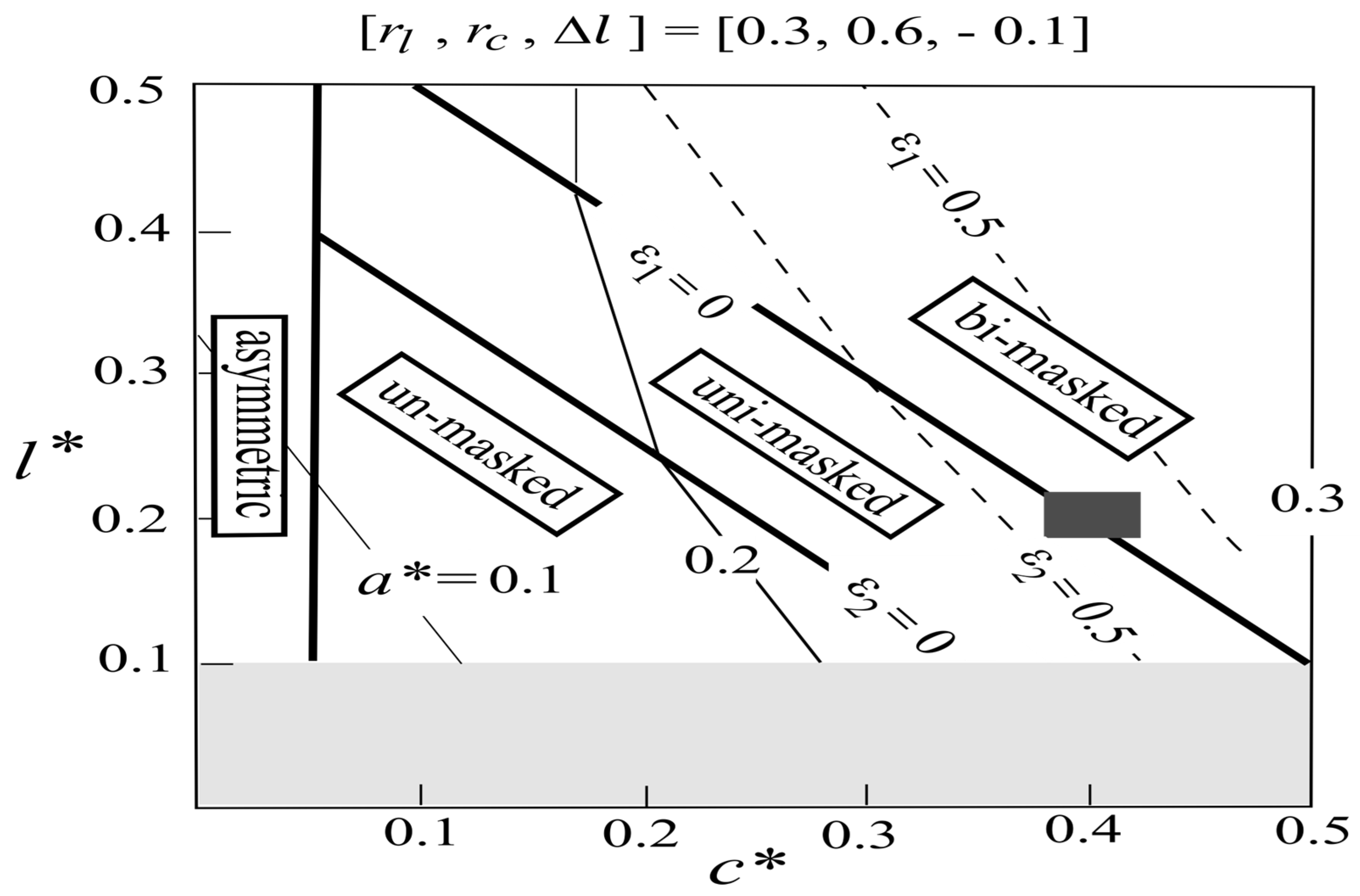
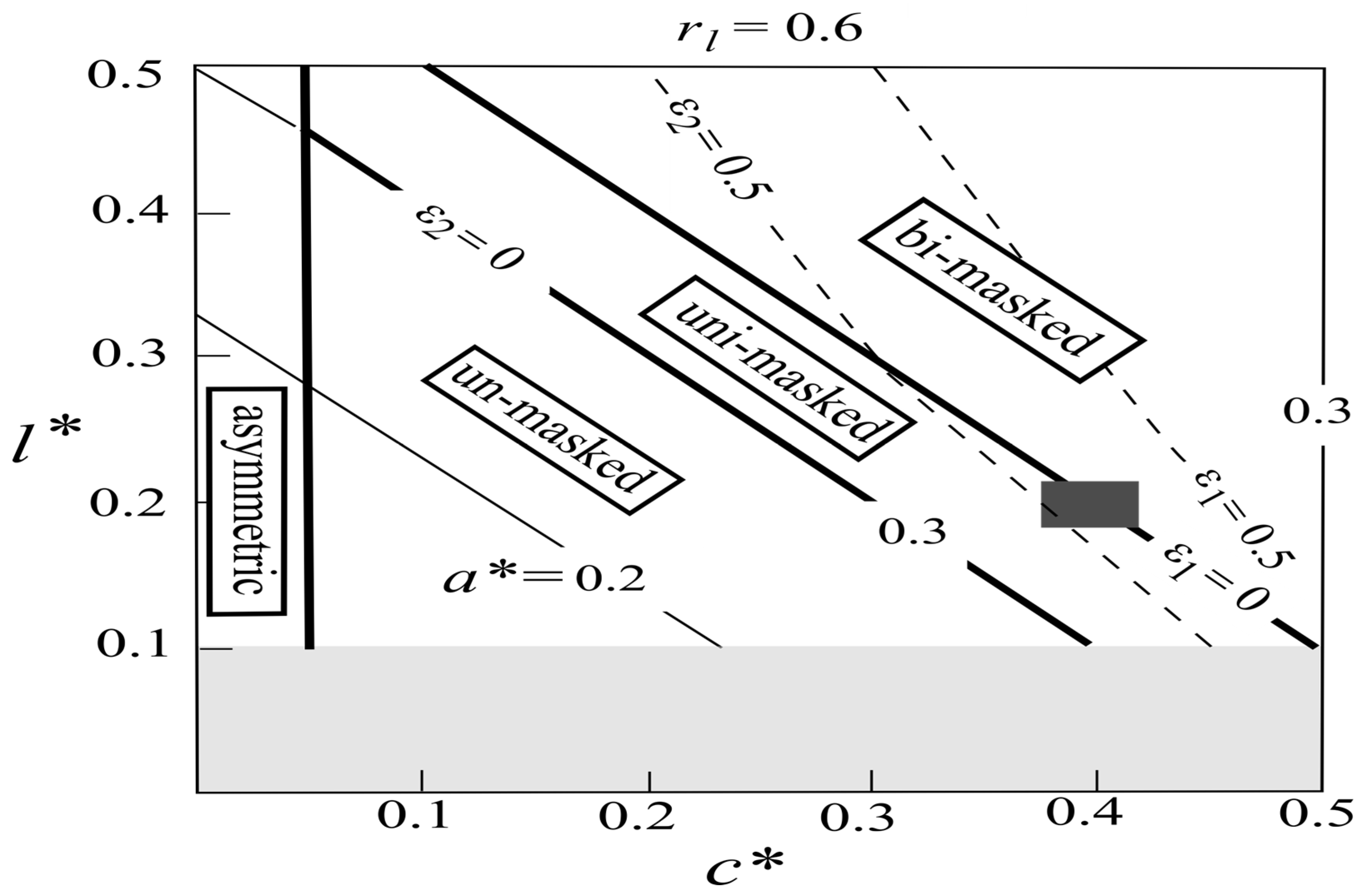
Subjected to (30), Equations (1), (2), (4) and (5) yield a tropical forcing of

$$q_0^{\prime }~q_0^{*}(1-2a_0)-q_1^{*}(1-4a_1),$$

(32)

whose maximization (28) has two immediate consequences. First, it minimizes the tropical albedo ($a_0$), so other than those generated by local processes, such as in the ITCZ and over the cooler eastern subtropical ocean, low-clouds that dominate the cloud albedo would be expelled to polar bands. As such, their polar-total

$$c^{*}=c_1+c_2$$

(33)

may be regarded as known from global balance (Section 1). Recalling that our polar bands consist of areas poleward of 30 latitudinal degrees, this deduction is highly discernable from observed stratus distribution [27] (their figure 2). Second, it maximizes the polar albedo ($a_1$), so the overlapped land/cloud areas

$${\epsilon }_i\mathrm{are}\mathrm{minimized}i=1,2.$$

(34)

That is, high-latitude stratus would saturate the ocean area before they mask the land, a deduction discernible from observation as well [28] (their figure 4).

3. Model Regimes

Having deduced the above tendency of cloud, I shall next prognose the quantitative albedo to be tested against observation. For this purpose, I summarize in Figure 2 the model regimes when the polar-total cloud increases from zero. The solid bars represent southern and (larger) northern lands, the open fluffy bars are clouds, and the two columns are their albedos and areas, respectively.

It is seen that only when the polar-total cloud albedo exceeds the asymmetry of the land albedo would the planetary albedo be symmetric, as indicated by the aligned dashed lines in the albedo column; the combined land/cloud areas (or ‘combined areas’ for short), however, remain unequal because of their differing reflectances. The symmetric regime is subdivided into three regimes depending on cloud-masking of the land (stripped): ‘un-masked’, ‘uni-masked’ (only the northern land) and ‘bi-masked’ (both polar lands), which are separated by their onset thresholds. Only in bi-masked regime when combined areas have saturated the band areas (that is, 1/4) would they be equal.

Like the cloud cover (33), we define the polar-total land by

$$l^{*}\equiv l_1+l_2,$$

(35)

and, based on following derivations, construct a regime diagram (Figure 3) spanned by the polar-total cloud/land areas $l^{*}/c^{*}$ for the standard case $\left[r_l,r_c,∆l\right]=[\mathrm{0.3,0.6},-0.1]$ (see Section 3.5). The four regimes and their dividing thresholds (thick solid lines) correspond to that depicted in Figure 2, and the calculated polar-total albedo $a^{*}$ and masking fractions ${\epsilon }_i$ are shown in thin solid/dashed lines, respectively. For the polar-total albedo, its 0.3 value overlies the right ordinate, and for the masking fraction, its zero/unity values align with the respective regime boundary and the right ordinate, respectively. The solid rectangle represents the current case, and the shaded region lies outside the model domain.

3.1. Asymmetric Regime

As seen in Figure 2a, the asymmetric regime is when the polar-total cloud albedo is smaller than the asymmetry of the land albedo, or

$$r_c{c}^{*}\le r_l\left|∆l\right|.$$

(36)

Defining the reflectance ratio

$$r\equiv r_l/r_c,$$

(37)

the threshold for the onset of the symmetric (un-masked) regime thus is

$$c_{un}^{*}=r\left|∆l\right|,$$

(38)

and, without the masked land, the polar-total albedo is simply

$$a^{*}=r_l{l}^{*}+r_c{c}^{*},$$

(39)

as plotted in Figure 3. For the standard case, the asymmetric regime is seen to be limited to cloud cover of less than 0.05, which is an order of magnitude smaller than the observed one, so for all practical purposes the polar albedo should be symmetric, which thus is a robust feature of MEP.

3.2. Un-Masked Regime

In the un-masked regime, the symmetric albedo (Figure 2b) implies

$$∆a=r_l∆l+r_c∆c=0,$$

(40)

so that

$$∆c=-r∆l,$$

(41)

or the asymmetric land albedo is wholly removed by the opposite asymmetry in the cloud albedo. The polar-total albedo (39) is shown in thin lines, which expectedly increases linearly with increasing polar-total cloud and land areas, but more strongly with the former because of the higher cloud reflectance.

The un-masked regime terminates when the larger sum of land/cloud areas has saturated the polar band, so the cloud, being confined to the polar band by MEP, would begin to mask the land. Because the cloud has smaller asymmetry than the land (41), this masking occurs first in the polar band with larger land (the northern one in the standard case). Since individual land/cloud areas can be expressed as

$$l_{\mathrm{1,2}}=(l^{*}\pm ∆l)/2,$$

(42)

and

$$c_{\mathrm{1,2}}=(c^{*}\pm ∆c)/2,$$

(43)

the cloud threshold for the onset of ‘uni’-masked regime thus satisfies

$$(l^{*}+\left|∆l\right|)/2+(c_{uni}^{*}-\left|∆c\right|)/2=1/4,$$

(44)

or, substituting from (41),

$$c_{uni}^{*}=1/2-l^{*}-(1-r)\left|∆l\right|,$$

(45)

as indicated by the thick line separating the uni-masked from the un-masked regimes.

3.3. Uni-Masked Regime

In the uni-masked regime, the masking fraction ${\epsilon }_2$ satisfies (see Figure 2c)

$$\left(1-{\epsilon }_2\right)l_2+c_2=1/4,$$

(46)

with the corresponding polar albedo

$$a_2=r_l\left(1-{\epsilon }_2\right)l_2+r_c{c}_2.$$

(47)

Since the southern land remains unmasked, its albedo is

$$a_1=r_l{l}_1+r_c{c}_1.$$

(48)

Eliminating masking fraction from (46) and (47) and equating (47) and (48) yields

$$∆c=\frac{r}{1-r/2}\left[\frac{1}{4}-\left(l_1+\frac{1}{2}{c}^{*}\right)\right],$$

(49)

which allows the calculation of $c_1$ and $c_2$ from (43), ${\epsilon }_2$ from (46) and polar-total albedo from twice of (48), as shown in Figure 3. From this expression, we see that an expanding cloud would be increasingly apportioned to the northern band to shade the excess land.

The uni-masked regime terminates when the sum of the southern land and cloud areas also attains 1/4 to enter the bi-masked regime. To derive this threshold, it is easier to first solve for the bi-masked regime and then determine its lower boundary.

3.4. Bi-Masked Regime

In the bi-masked regime, the southern masking fraction ${\epsilon }_1$, as its northern counterpart (46), satisfies

$$\left(1-{\epsilon }_1\right)l_1+c_1=1/4,$$

(50)

with the corresponding albedo

$$a_1=r_l\left(1-{\epsilon }_1\right)l_1+r_c{c}_1.$$

(51)

Eliminating both masking fractions from (47) and (51) yields

$$a_i=r_l/4+(r_c-r_l)c_{i}i=1,2,$$

(52)

and equating them on account of the symmetry yields

$$∆c=0,$$

(53)

so that

$$c_i=c^{*}/2i=1,2.$$

(54)

That is, since both polar bands are saturated by the combined area, the albedo symmetry demands the same cloud and exposed land areas, as seen in Figure 2d. As the cloud is now evenly partitioned between polar bands, its removal of the land asymmetry is not by opposite asymmetry, as in the un-masked regime, but by its equalization of the exposed land area. The masking fractions of the two bands can be calculated from (46) and (50) and polar-total albedo from (52), as shown in Figure 3. Since the asymmetric land has dived under cloud, the polar-total albedo no longer senses the land asymmetry, as seen in its vertical orientation.

Setting ${\epsilon }_1=0$ in (50), we derive the cloud threshold for the onset of the bi-masked regime

$$c_{bi}^{*}=1/2-l^{*}+\left|∆l\right|.$$

(55)

In contrast to uni-masked threshold (45), it is a function only of the smaller polar land ($l_1$), independent of the reflectance: the smaller this land, the greater the cloud threshold before it is masked.

3.5. Parameter Dependence

The solid rectangle in Figure 3 represents the current condition based on the following sources. From [29] (their figure 1.12), we set the land partitions $\left[l_0,l_1,l_2\right]=\left[\mathrm{0.1,0.05,0.15}\right]$, so the land occupies 30% of the global surface with a polar-total of $l^{*}=0.2$; the northern polar land is three times the southern one, so the hemispheric asymmetry is $∆l=-0.1$, as seen in the blocked-out domain (the land area cannot be negative). With the cloud albedo dominated by stratus, we set its polar-total $c^{*}=0.4$ gleaned from [27] (their figure 2) and its reflectance $r_c=0.6$ [29] (their table 3.2). We set the land reflectance $r_l=0.3$, which consists of 0.2 from land [29] (their table 4.2) and 0.1 from aerosol [30].

These ‘standard’ values would produce a clear-sky asymmetry of 10 $\mathrm{W}{\mathrm{m}}^{-2}$ in the reflected SW flux (smaller if we use the higher reflectance of Antarctica), which is observed to be removed by clouds to within 0.3 $\mathrm{W}{\mathrm{m}}^{-2}$ of the above flux or ${10}^{-4}$ in the planetary albedo. Such precision obviously cannot be due to the atmospheric dynamics given its vagaries, but rather, as I contend, reflects an inexorable march toward MEP by thermodynamics. Since the standard case falls around the bi-masked threshold, the cloud cover would be evenly divided between polar bands, so its mitigation of the land asymmetry is largely through shading the excess northern land. On the other hand, given the crudeness of the model, the standard case could veer into the uni-masked regime to render a slightly cloudier southern hemisphere, as seems the observed case [2], which, according to our model, however is insufficient to symmetrize the albedo without shading the land.

The calculated polar albedo is 0.27, to which cloud contributes 0.24 and land 0.03, where the latter represents a halving of its clear-sky value to render an order of magnitude difference between the two contributions. With the deduced cloud tendency, the tropical albedo is due primarily to land (high clouds over the ITCZ has little reflectance, [22]) hence has a value of $r_l{l}_0=0.03$ to yield a total albedo of 0.3. All these values are commensurate with observed ones [1,5], which is somewhat surprising considering the crudeness of our box model.

To assess parameter dependence of the modelled albedo, I consider two extreme cases, which nonetheless are realized in paleohistory hence of practical relevance. The first is the ice age when the polar land is as reflective as the cloud. Setting $r_l=0.6$, the regime diagram is shown in Figure 4, which can be compared with the current interglacial shown in Figure 3. Expectedly, the augmented land reflectance has rotated the albedo lines counterclockwise to become more diagonal, and the albedo attains a uniform value (0.3) in masked regimes. While the icy surface has raised the planetary albedo, the increase is only 10% since the exposed land is relatively small compared with the cloud cover (0.1 vs. 0.4). Since the symmetric regimes are characterized by equalized albedos as well as combined areas, the uni-masked threshold is slightly higher, but the bi-masked threshold remains unchanged. As such, only the northern land is slightly less masked, but the southern land remains largely exposed.

The second extreme case is when the polar land is symmetric, which can be representative of Pangea in the early Triassic period when it extends from pole to pole [31]. Setting the land partitions $\left[l_0,l_1,l_2\right]=\left[\mathrm{0.1,0.1,0.1}\right]$, the regime diagram is shown in Figure 5. Naturally, all vestiges of asymmetry are eliminated, including the disappearance of the asymmetric and uni-masked regimes. Compared with the standard case, the albedo retains the same value (0.27) and has the same land/cloud contributions, but the southern masking is strongly expanded to equal the northern one.

Based on the model solution of these extreme cases, the present polar albedo is only slightly augmented during the ice age of more reflective land and remains unchanged during the early Triassic of symmetric land. Although the polar albedo is relatively stable because of its dominance by vast low-clouds, the global albedo can be strongly altered by the varying tropical land not considered here.

4. Conclusions

I posit that the climate, with clouds as its internal component, is a macroscopic manifestation of a NT system to be governed by MEP, a generalized second law. Through a minimal box model, I show that low-clouds, which dominate the cloud albedo, would be expelled to high latitudes to equalize the hemispheric planetary albedo—a remarkable observation, which may now be explained. Moreover, because of vastness of the low-clouds, their compensation of the land asymmetry is not by an opposite asymmetry but primarily by masking the excess land, a deduction consistent with observation. When the model is applied to the ice age of highly reflective land and the early Triassic period of symmetric land, the polar albedo is only slightly altered from the present, suggesting its considerable stability through Earth’s history.

Climate models fall far short in replicating the observed albedo symmetry and the intermodel spread of calculated clouds has not narrowed in past decades despite much expanded physics [32]. With the demonstrated potency of MEP in propelling the cloud, the present study suggests an alternative strategy in improving climate models, namely by reappropriating computing resources from detailed physics to resolving eddies, thereby encapsulating the NT.

References

1. Stephens, G.L.; O’Brien, D.; Webster, P.J.; Pilewski, P.; Kato, S.; Li, J.L. The albedo of Earth. Rev. Geophys. 2015, 53, 141–163. [Google Scholar] [CrossRef] [Green Version]
2. Datseris, G.; Stevens, B. Earth’s albedo and its symmetry. AGU Adv. 2021, 2, e2021AV000440. [Google Scholar] [CrossRef]
3. Voigt, A.; Stevens, B.; Bader, J.; Mauristen, T. The observed hemispheric symmetry in reflected shortwave irradiance. J. Clim. 2013, 26, 468–477. [Google Scholar] [CrossRef]
4. Haywood, J.M.; Jones, A.; Dunstone, N.; Milton, S.; Vellinga, M.; Bodas-Salcedo, A.; Hawcroft, M.; Kravitz, B.; Cole, J.; Watanabe, S.; et al. The impact of equilibrating hemispheric albedos on tropical performance in the HadGEM2-ES coupled climate model. Geophys. Res. Lett. 2016, 43, 395–403. [Google Scholar] [CrossRef] [Green Version]
5. Donohoe, A.; Battisti, D.S. Atmospheric and surface contributions to planetary albedo. J. Clim. 2011, 24, 4402–4418. [Google Scholar] [CrossRef]
6. Kang, S.M.; Held, I.M.; Frierson, D.M.W.; Zhao, M. The response of the ITCZ to extratropical thermal forcing: Idealized slab-ocean experiments with a GCM. J. Clim. 2008, 21, 3521–3532. [Google Scholar] [CrossRef] [Green Version]
7. Donohoe, A.; Marshall, J.; Ferreira, D.; Mcgee, D. The relationship between ITCZ location and cross-equatorial atmospheric heat transport: From the seasonal cycle to the Last Glacial Maximum. J. Clim. 2013, 26, 3597–3618. [Google Scholar] [CrossRef]
8. Voigt, A.; Stevens, B.; Bader, J.; Mauritsen, T. Compensation of hemispheric albedo asymmetries by shifts of the ITCZ and tropical cloud. J. Clim. 2014, 27, 1029–1044. [Google Scholar] [CrossRef]
9. Ozawa, H.; Ohmura, A.; Lorenz, R.D.; Pujol, T. The second law of thermodynamics and the global climate system: A review of the maximum entropy production principle. Rev. Geophys. 2003, 41, 1018. [Google Scholar] [CrossRef] [Green Version]
10. Kleidon, A. Non-equilibrium thermodynamics and maximum entropy production in the Earth system: Applications and implications. Naturwissenschaften 2009, 96, 653–677. [Google Scholar] [CrossRef] [Green Version]
11. Dewar, R.C.; Lineweaver, C.H.; Niven, R.K.; Regenauer-Lieb, K. Beyond the second law: An overview. In Understanding Complex Systems; Springer: Berlin/Heidelberg, Germany, 2014; pp. 3–27. [Google Scholar] [CrossRef]
12. Ou, H.W. Thermohaline circulation: A missing equation and its climate change implications. Clim. Dyn. 2018, 50, 641–653. [Google Scholar] [CrossRef]
13. Evans, D.J.; Cohen, E.G.; Morriss, G.P. Probability of second law violations in shearing steady states. Phys. Rev. Lett. 1993, 71, 2401–2404. [Google Scholar] [CrossRef] [PubMed] [Green Version]
14. Wang, G.M.; Sevick, E.M.; Mittag, E.; Searles, D.J.; Evans, D.J. Experimental demonstration of violations of the second law of thermodynamics for small systems and short time scales. Phys. Rev. Lett. 2002, 89, 050601. [Google Scholar] [CrossRef] [Green Version]
15. Shimokawa, S.; Ozawa, H. On the thermodynamics of the oceanic general circulation: Irreversible transition to a state with higher rate of entropy production. Q. J. R. Meteorolog. Soc. 2002, 128, 2115–2128. [Google Scholar] [CrossRef]
16. Kleidon, A.; Fraedrich, K.; Kunz, T.; Lunkeit, F. The atmospheric circulation and states of maximum entropy production. Geophys. Res. Lett. 2003, 30, 2223. [Google Scholar] [CrossRef]
17. Fraedrich, K.; Lunkeit, F. Diagnosing the entropy budget of a climate model. Tellus 2008, A60, 921–931. [Google Scholar] [CrossRef] [Green Version]
18. Hogg, A.M.; Gayen, B. Ocean gyres driven by surface buoyancy forcing. Geophys. Res. Lett. 2020, 47, e2020GL088539. [Google Scholar] [CrossRef]
19. Colin de Verdière, A. Buoyancy driven planetary flows. J. Mar. Res. 1988, 46, 215265. [Google Scholar] [CrossRef]
20. Ou, H.W. Possible bounds on the earth’s surface temperature: From the perspective of a conceptual global-mean model. J. Clim. 2001, 14, 2976–2988. [Google Scholar] [CrossRef]
21. Crowley, T.J.; North, G.R. Paleoclimatology; Oxford University Press: New York, NY, USA, 1991; 339p. [Google Scholar]
22. Liou, K.N. (Ed.) Chapter 8—Radiation and Climate; Int Geophys, Academic Press: Cambridge, MA, USA, 2002; Volume 84, pp. 442–521. ISSN 0074-6142. [Google Scholar]
23. Kim, D.; Ramanathan, V. Solar radiation and radiative forcing due to aerosols. J. Geophys. Res. 2008, 113, D02203. [Google Scholar] [CrossRef] [Green Version]
24. Pauluis, O.; Held, I.M. Entropy budget of an atmosphere in radiative-convective equilibrium. Part I: Maximum work and frictional dissipation. J. Atmos. Sci. 2002, 59, 125–139. [Google Scholar] [CrossRef]
25. Ou, H.W. Hydrological cycle and ocean stratification in a coupled climate system: A theoretical study. Tellus 2007, 59A, 683–694. [Google Scholar] [CrossRef] [Green Version]
26. Peixoto, J.P.; Oort, A.H. Physics of Climate; American Institute of Physics: New York, NY, USA, 1992; 520p. [Google Scholar]
27. Klein, S.A.; Hartmann, D.L. The seasonal cycle of low stratiform clouds. J. Clim. 1993, 6, 1587–1606. [Google Scholar] [CrossRef]
28. Wood, R. Stratocumulus Clouds. Mon. Weather. Rev. 2012, 140, 2373–2433. [Google Scholar] [CrossRef]
29. Hartmann, D.L. Global Physical Climatology; Academic Press: New York, NY, USA, 2015; 411p. [Google Scholar]
30. Ramanathan, V.C.; Crutzen, P.J.; Kiehl, J.T.; Rosenfeld, D. Aerosols, climate, and the hydrological cycle. Science 2001, 294, 2119–2124. [Google Scholar] [CrossRef] [Green Version]
31. Scotese, C.R.; Golonka, J. Paleogeographic Atlas; PALEOMAP project, Department of Geology, University of Texas at Arlington: Arlington, TX, USA, 1993. [Google Scholar]
32. Stephens, G.L. Cloud feedbacks in the climate system: A critical review. J. Clim. 2005, 18, 237–273. [Google Scholar] [CrossRef] [Green Version]
Figure 1. Model configuration in which the coupled ocean/atmosphere is divided into symmetric tropical/polar-bands of equal area, tagged numerically by 1/0/2 proceeding north. The external forcing is the symmetric incident SW flux ( q * ), which is reflected by land (l) and cloud (c) before absorbed by the ocean (q). The ocean heats the atmosphere differentially via the convective flux ( q c ) proportional to the sea/air temperature difference ( T T a ) and the heat exits the system via outgoing LW flux ( q O L R ).
Atmosphere 14 01243 g001
Figure 2. Model regimes with increasing polar-total cloud cover, as illustrated by albedos and areas of land/cloud (solid/open bars). The symmetric albedo regime is subdivided into un-, uni- and bi-masked regimes depending on cloud masking of the polar land (striped) separated by their onset thresholds.
Atmosphere 14 01243 g002
Figure 3. The regime diagram spanned by the polar-total land/cloud areas l * / c * for the ‘standard’ case r l , r c , l = [ 0.3,0.6 , 0.1 ] . The four regimes and their dividing thresholds (thick solid lines) correspond to that depicted in Figure 2 with calculated polar-total albedo a * and masking fractions ε i contoured in thin solid/dashed lines, respectively. The solid rectangle represents the current case, and the shaded region lies outside the model domain.
Atmosphere 14 01243 g003
Figure 4. Same as Figure 3, but for the higher land reflectance r l = 0.6 of the ice age, which shows diagonal albedo lines and slightly less masked northern land.
Atmosphere 14 01243 g004
Figure 5. Same as Figure 4, but for symmetric land l = 0 as during the early Triassic period, which has removed all asymmetries and the albedo retains a similar value as the standard case.
Atmosphere 14 01243 g005
Disclaimer/Publisher’s Note: The statements, opinions and data contained in all publications are solely those of the individual author(s) and contributor(s) and not of MDPI and/or the editor(s). MDPI and/or the editor(s) disclaim responsibility for any injury to people or property resulting from any ideas, methods, instructions or products referred to in the content.