Article

Assessment of Multifractal Fingerprints of Reference Evapotranspiration Based on Multivariate Empirical Mode Decomposition

1
TKM College of Engineering, Kollam 691005, India
2
Department of Research in Geoscience, KaruSphère SASU, 97139 Abymes, Guadeloupe, France
3
Faculty of Civil Engineering, University of Tabriz, Tabriz 5166616471, Iran
4
World Peace University, Sht. Kemal Ali Ömer Sok. Tower 305, Yenişehir, Nicosia, TRNC, Mersin 10, Lefkoşa 99010, Turkey
*
Authors to whom correspondence should be addressed.
Atmosphere 2023, 14(8), 1219; https://doi.org/10.3390/atmos14081219
Submission received: 29 June 2023 / Revised: 22 July 2023 / Accepted: 25 July 2023 / Published: 28 July 2023
(This article belongs to the Section Meteorology)

Abstract

:
This study analyzed the multifractal characteristics of daily reference evapotranspiration (ETo) time series of the Tabriz and Urmia stations of northwestern Iran and its cross-correlation with five other meteorological variables. The results of multifractal detrended fluctuation analysis (MFDFA) of ETo, temperature, pressure, relative humidity solar radiation, and wind velocity showed that all the time series of both stations exhibited multifractality and long memory persistence with higher persistence and complexity in the datasets of Urmia station. Then, a multivariate empirical mode decomposition (MEMD)-(MFDFA) coupled framework was proposed to identify the dominant modes suitable for the forecasting of the different variables. The examination of reconstructed time series consistently displayed an increase in persistence and multifractality. The cross-correlation between different candidate variables and ETo was examined using a recently proposed multifractal cross-correlation analysis (MFCCA) method. The results showed that in each pair-wise cross-correlation analysis, the joint persistence is approximately half of the persistence of an individual time series, reinforcing the universality in the fractal cross-correlation analysis. The cross-correlation properties displayed diverse patterns in different pair-wise combinations of cross-correlation analysis despite the similarity of patterns among the data of the two stations.

1. Introduction

Evapotranspiration (ET) is one of the prominent components of a hydrologic cycle, and its accurate prediction is vital in irrigation and water resources management. The rate of ET from a reference crop of 0.12 m height, bulk surface resistance of 70 sm−1, and albedo of 0.23, assuming a surplus of soil moisture, is called reference evapotranspiration (ETo) [1], is perhaps the most tangible form of evapotranspiration in the analysis of a hydrologic cycle. ETo is often controlled by numerous meteorological variables, and the inherent complexities of such variables often force researchers to search for diverse methods, ranging from statistical to machine learning, for accurate modeling [2,3]. Hydro-climatic time series often possess nonlinear and nonstationary characteristics with the presence of trends, shifts, and abrupt fluctuations, which are also exhibited in the ETo time series. The characterization of a time series and the examination of its long-term dependency is crucial for the accurate modeling of the process [4]. Hurst proposed the rescaled range (R/S) analysis as one of the initial contributions to the persistence of a time series [4]. Mantelbrot [5] presented the theory of fractality, which determines that on subdividing a geometrical object into parts, each part will be a downscaled copy of the object. Fractality is closely linked with persistence, and a considerable number of algorithms have been proposed for estimating the fractal behavior of the time series. The Fourier spectral method [6], wavelet-based analysis [7], arbitrary order Hilbert spectral analysis (AOHSA) [8], structure function [9,10], and visibility graph analysis [11,12] are among them. Peng et al. [13] proposed a robust technique, namely detrended fluctuation analysis (DFA), for analyzing the fractality based on a detrending operation. Kantelhardt et al. [14] propounded the multifractal (MF) extension of DFA (so-called MFDFA). The multifractal parameters can be considered as ‘fingerprints’ of the series, as they are useful in modeling [15].
In the past two decades, numerous studies on the multifractal analysis of hydro-climatic data were performed using MFDFA [16,17,18,19,20,21,22]. Multifractal properties were also detected in meteorological time series, such as temperature, wind velocity, solar radiation, and relative humidity, in different parts of the world [23,24,25,26,27,28]. Baranowski et al. [29] analyzed the scaling properties of the time series of temperature, wind speed, relative humidity, rainfall, and solar radiation comprising over 11,000 points from stations in Germany, Finland, Spain, and Poland. Long-range correlations were the reasons for the multifractality of the majority of the series, except for rainfall. Krzyszczak et al. [27] used MFDFA to analyze the multifractal properties of the meteorological datasets of four stations in Poland and Bulgaria located in varying climatic zones. They have analyzed daily time series comprising more than 11,000 observations of temperature, rainfall, relative humidity, and wind speed. It was revealed that the multifractal characteristics of rainfall are quite different from those of others. Entire time series were partitioned at about 2001–2002, and the multifractal characteristics were analyzed to evaluate the differences in dynamics. The multifractal spectrum was found to be susceptible to climatic shift, and it was especially apparent for asymmetry, which changed from being right to left skewed, implying more extreme events in the recent past.
Evapotranspiration is a complex process that happens as a visible natural outcome of the concurrent interactions of different meteorological variables. The modeling of any hydrologic variable is a challenging problem for a hydrologist, for which either a time-series approach, a cause–effect approach, or a combined approach involving the two can be followed. Several methods have been proposed in the past for modeling reference-crop ETo including mass transfer, water budget, pan evaporation, radiation, and temperature-based methods, as well as the recent practices of data-driven methods [30,31]. Recently, Sreedevi et al. [32] investigated the teleconnection between the meteorological variables and reference ETo of Urmia and Tabriz of northwestern Iran in a multi-scale perspective. The region is hydro-climatologically sensitive and of ecological importance because of the presence of Lake Urmia, and it is important to investigate the impact of different climate regimes on the modeling of hydrological variables. Identifying the most appropriate predictor variables and understanding the joint association between the influential variables with Eto are among the key steps in the more popular cause–effect approach of modeling evapotranspiration. According to the authors’ knowledge, even though many studies have been proposed for evaluating the fractal properties of hydrological variables employing the MFDFA procedure, the study on the multifractal characterization of evapotranspiration is scarce in the literature [2,20,33]. Ariza-Villaverde et al. [34] used joint multifractal analysis for examining the association between temperature, relative humidity, and ETo of Cordoba city in Spain. Multifractal characterization of daily ETo in different climate zones of China was performed by Zhan et al. [35]. Gómez-Gómez et al. [36] analyzed the cross-correlation between the meteorological variables and ETo of the Guadalquivir River Valley using the multifractal detrended cross-correlation method.
The objectives of this paper include (i) analyzing the multifractality daily ETo time series and five other climate variables (temperature, pressure, relative humidity, wind velocity, and solar radiation) of two stations located in northwestern Iran, (ii) proposing an MEMD-MFDFA method for the identification of the dominant modes for the prediction of candidate variables, and (iii) investigating the cross-correlation between ETo and the five climate variables using multifractal cross-correlation analysis (MFCCA).

2. Study Area and Observation Data

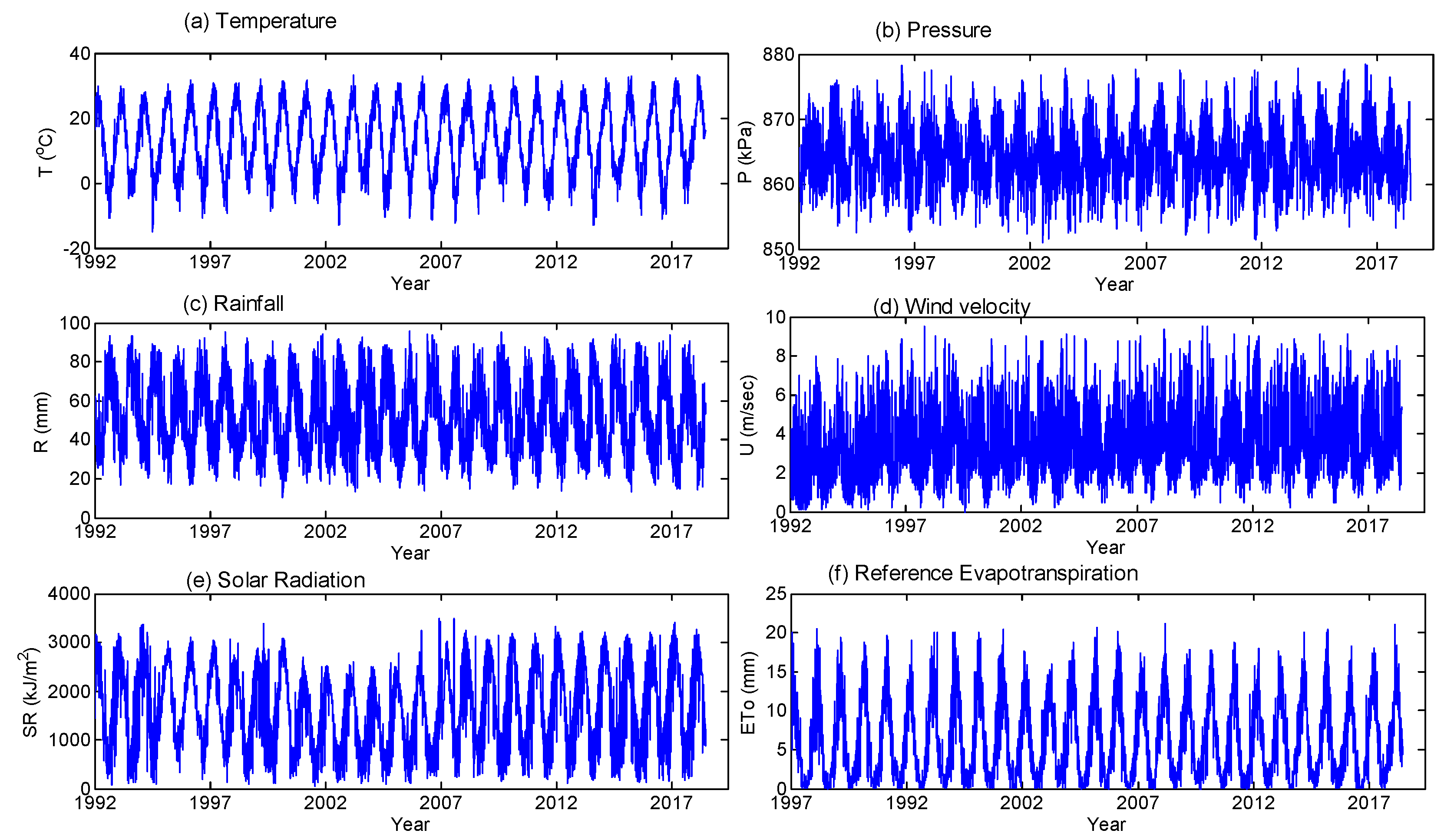
In this study, temperature (T) (°C), pressure (P) (kPa), wind velocity (U) (ms−1), relative humidity (RH) (%), solar radiation (SR) (kJ m−2), and ETo (mm) at daily time scales obtained from the two stations at Tabriz and Urmia cities were considered for the multifractal analysis (June 1992 to October 2018 for Tabriz and June 1992 to October 2016 for Urmia). The positions of the stations are given in Figure 1. Tabriz city, which has a mean altitude of 1350 m, is located between latitudes 38°8′ N and 46°15′ E at the intersection of the Aji and Quri rivers. Tabriz has a rainfall of about 378 mm annually; it experiences a dry to semi-hot summer and a mild climate in spring. The mean temperature is nearly 14 °C per year with a rate of ET around 1740 mm/year. Urmia is located at 37°34′ N and 44°58′ E in northwestern Iran at an average altitude of 1332 m. Urmia experiences scanty summer rainfall and heavy rainfall in winter. In most years, freezing occurs over four months. The annual rainfall of the station is nearly 310 mm [37]. Time-series plots of the data for Tabriz and Urmia used in this study are shown in Figure 2 and Figure 3.
The quick reception of solar irradiance results in the rise in temperature and the subsequent increase in ET. Therefore, Tabriz records a higher maximum pan evaporation and maximum temperature (15 mm/day and 35 °C, respectively) than Urmia (11 mm/day and 34 °C). However, because of Lake Urmia, evaporation will be higher in that region, leading to higher maximum and average daily rainfall (3.8 mm and 0.7 mm, respectively) than in Tabriz (3 mm and 0.6 mm). The statistical properties of the hydro-meteorological data of the Tabriz and Urmia stations are stated in Table 1.

3. Materials and Methods

3.1. Multifractal Detrended Fluctuation Analysis (MFDFA)

MFDFA is a well-established algorithm for detecting the scaling behaviors and multifractality of nonlinear and nonstationary datasets. This method involves (i) the computation of a profile by subtracting each value in the time series from its mean, (ii) the division of the profiles into segments of different lengths (so-called scale, s) and the polynomial fitting for each of them, (iii) estimating the local trend by taking the difference of the segment from the fitted polynomial, for each moment order (q), by the aggregation and averaging of operations, and (v) performing a logarithmic fit between the fluctuation function to obtain the generalized Hurst exponents (GHE) for different moment orders, and this value for moment order q = 2 is quite similar to the classical Hurst exponent, which can provide information on the persistence of the time series. Then, based on the plot between GHE and the q-order, one can comment on the fractality of the time series, i.e., whether it is monofractal or multifractal. Subsequently, the multifractal spectrum can be derived, which can provide useful insights into the multifractal strength of the series. More details on the algorithm are provided in Appendix A.

3.2. Multifractal Cross-Correlation Analysis (MFCCA)

The mutual association between different hydrologic and climatic variables was traditionally analyzed using a correlation coefficient (R). However, the R value may be misleading if outliers are present and it is only deciphering the linear association between the variables. Podobnik and Stanley [38] propounded the detrended cross-correlation analysis (DCCA) to analyze the power-law cross-correlations between the two signals. Extension of DCCA to a multifractal domain was made by researchers via the proposal of multifractal DCCA [39], multifractal detrending moving-average cross-correlation analysis (MFXDMA) [40], and multifractal cross-correlation analysis (MFCCA) [41]. These improvisations have been applied to time series from different scientific fields [2,20,33,42,43]. The steps of MFCCA are as follows:
  • Consider two time-series signals, xi and yi (i = 1,2,…,N), to find their profiles:
    X p ( j ) = i = 1 j [ x i x m ]
    and
    Y p ( j ) = i = 1 j [ y i y m ]
    where i = 1,2,……., N; xm and ym are the mean of the respective signals.
  • Divide the series into Ns independent windows, both in progressive and retrograde orders (hence, 2Ns), to avoid any exclusion of data points at the head and tail ends.
  • For each window, compute the local trends by fitting an m-order polynomial:
    f f X Y 2 ( v , s ) = 1 s k = i s [ X ( ( v 1 ) + k ) p X , ν m ( k ) × Y ( ( v 1 ) + k ) p Y , ν m ( k ) ]
  • Estimate the detrended covariance:
    F q X Y ( s ) = 1 2 N s υ = 0 2 N s 1 s i g n [ f f X Y 2 ( υ , s ) ] | f f X Y 2 ( υ , s ) | q / 2
    where FqXY(s) is the fluctuation function (FFn), bearing the relation:
    FqXY(s) ~ sλ(q)
    where s is the segment size.
The exponent λ(q) is similar to the GHE in MFDFA. Unlike DCCA, it is a method that also accounts for the sign of FFn of different statistical moment orders. The modifications of Equations (3) and (4) for backward computations and q = 0 can be found in the literature [44].
The coefficient ρXY is coined as the ratio between the covariance function F X Y and the variance functions F X and F Y after detrending [45]:
ρ X Y = F q X Y F q X F q Y
ρXY range [−1,1], (±0.66 to ±1) indicates high, (±0.33 to ±0.66) is moderate, and (zero to ±0.33) is low [46]. The MFCCA analysis can provide a better physical insight, as it indicates the scale-specific correlation between two variables, which computes the covariance function of two time series along with the signs [47,48].

3.3. Multivariate Empirical Mode Decomposition (MEMD)

Empirical mode decomposition (EMD) is a data-based decomposition technique provided by Nordan E. Huang in 1998, which decomposes a signal into enough modes with definite periodicity and is based on spline fitting through the extremes (crest and trough points) of the signal. The multivariate EMD propounded by Rehman and Mandic [49] is an extended version of EMD, which can decompose more than three signals concurrently by tracking the common scales in them. Here, multiple envelopes are developed by finding the projections of inputs along various directions in an n-D space. Let V ( t ) = { V 1 ( t ) , V 2 ( t ) V n ( t ) } be the m variable signals and D V θ d = { D 1 d , D 2 d , , D n d } denote the direction vectors (DVs) defined by angles θ d = { θ 1 d , θ 2 d , θ n 1 d } in direction set DV (d = 1,2,3,…D), where D is the number of directions. It is noteworthy to state that instead of there being oscillatory modes in EMD, rotational modes are generated in MEMD.
The mean zero rotation components (called intrinsic mode functions or IMFs) can be obtained by the following steps:
  • Generating appropriate sets of DVs by sampling on a (n − 1) unit hypersphere;
  • Computing the projections p θ d ( t ) of V(t) along the DVs D V θ d for all d;
  • Finding the time instants t i θ d of the maxima of projections for all d;
  • Interpolating [ t i θ d , D ( t i θ d ) ] to get the surface E θ d ( t ) for all d;
  • Finding the mean of surfaces:
    S ( t ) = 1 K k = 1 K E θ d ( t )
  • Extracting R(t) = V(t) − S(t). If R(t) satisfies the termination criteria, repeat from (1) onward upon (V(t) − R(t)), otherwise repeat from (2) upon the reminder R(t).
This method has many advantages over conventional EMD, as it provides cleaner decomposition and spectral representation of the signals, ensures an equal number of components for different candidate series by recognizing the scales commonly present, and is easier to implement [49,50,51]. The Hammersley sampling scheme is suitable for generating DVs, and the Cauchy-type termination criteria is suitable for implementing the algorithm [51]. MEMD is used as a data-processing tool in a hybrid modeling framework for modeling hydrological variables including evapotranspiration [52,53,54]. This study proposes the use of MEMD instead of conventional EMD, for identifying the dominant modes, which can improve the predictability of the time series [55].
The MEMD algorithm can decompose any complex time series into a definite number of IMFs of specific frequency and end residual. In general, the modes are arranged in descending order of their frequencies, with the mode of highest frequency IMF at the top. In the practical hydrological signals, there is a good chance that some of the modes, like high-frequency IMFs, may contain noise, which may affect the performance in predictions. Hence, the elimination of the noise-intruded component is very important in improving the predictability of the hydrological signals.

3.4. MEMD-MFDFA Framework for Reconstruction

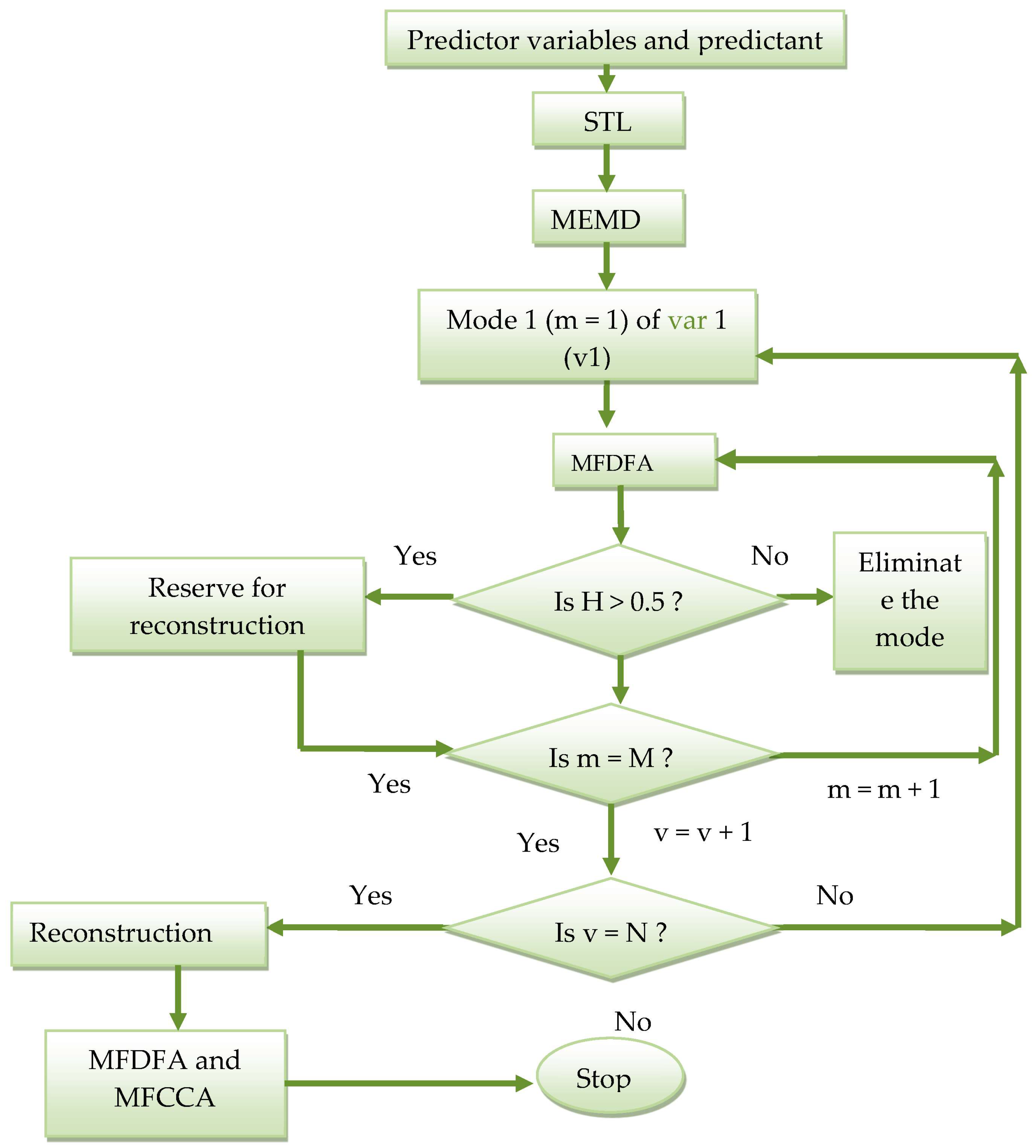
An MFDFA-based approach is proposed for identifying the less-contributing signals. The different steps of this framework are presented in Figure 4.
Most of the EMD-based de-noising methods in the past considered the highest frequency mode only (IMF1) as noise [55], and in this procedure, we consider both Gaussian white noise and anti-persistent processes by fixing a threshold H of 0.5.

4. Results and Discussion

In this section, the results of the MFDFA analysis performed on different time-series data collected from the Tabriz and Urmia stations are provided first. Then, the results of the reconstructed time series using the proposed MEMD-MFDFA framework are presented, followed by the results of the MFDFA analysis of the reconstructed data. In the final subsection, the results of the cross-correlation analysis between different variables and ETo are presented.

4.1. MFDFA of ETo and Meteorological Variables

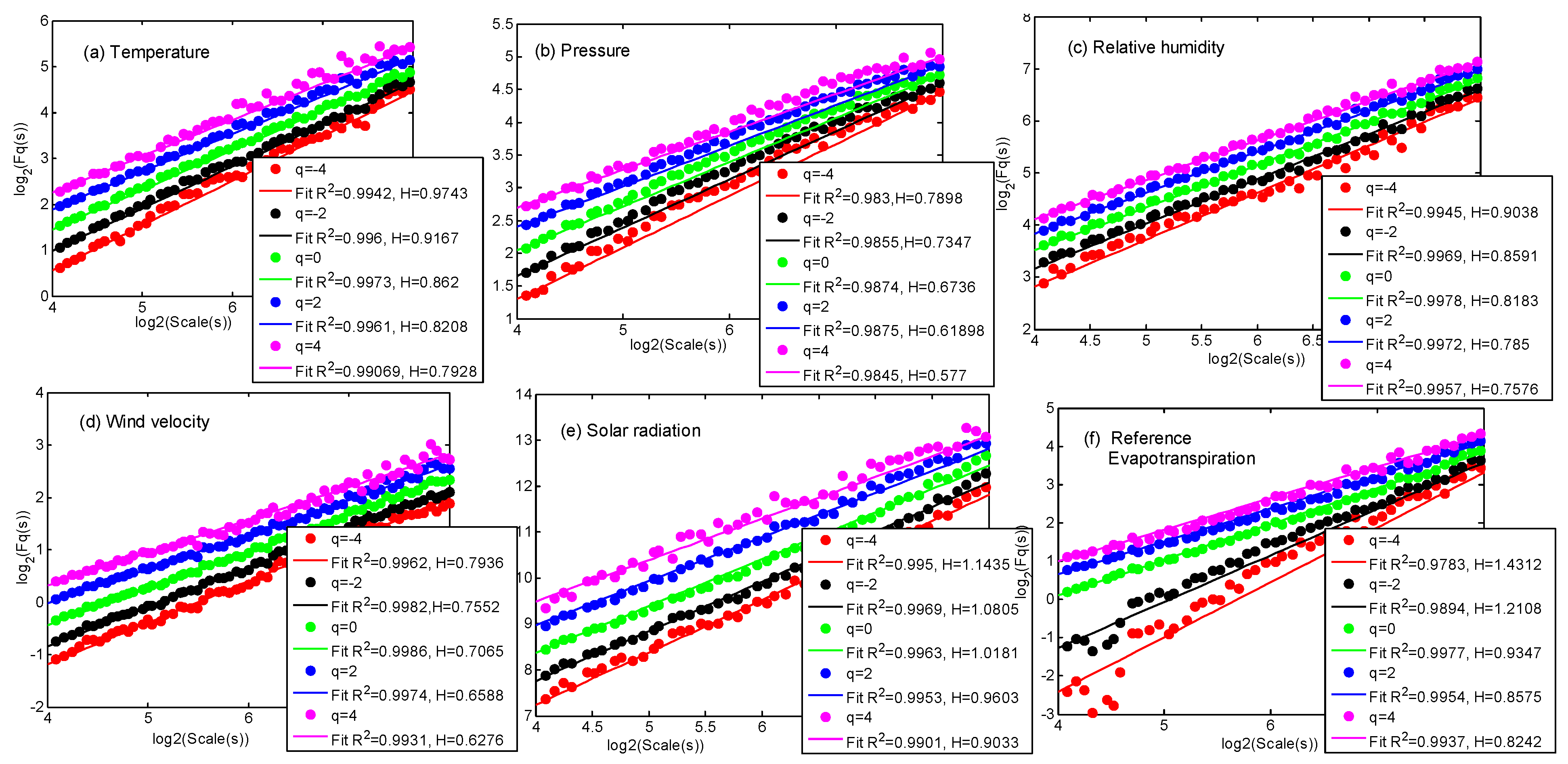
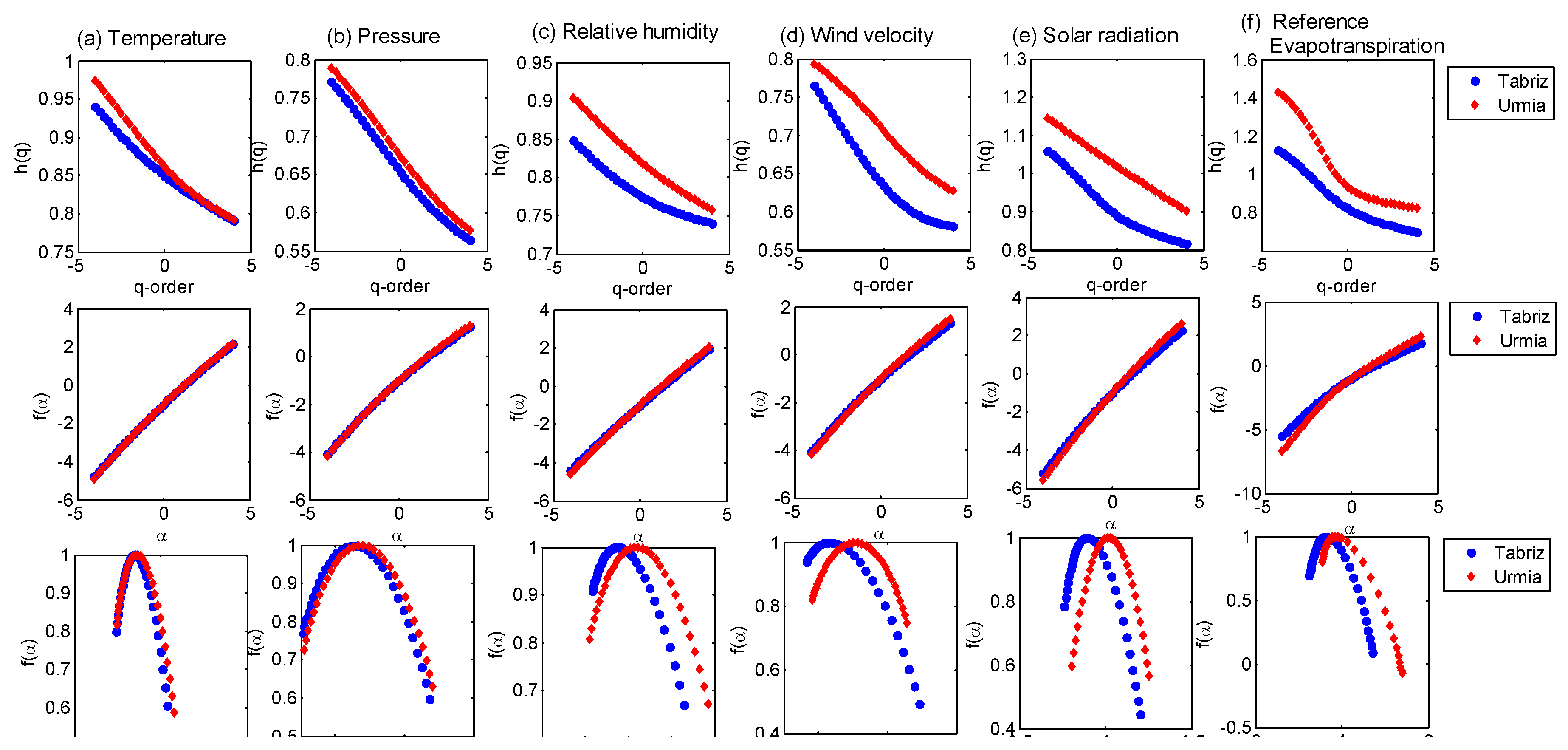
In the MF-DFA framework, the presence of seasonality in a time series is associated with potential crossovers in the log–log plots of Fq(s) vs. s [28]. This characteristic can significantly impact the results and their interpretation, primarily because of the existence of different scaling regimes in the multifractal properties. An effective approach to removing seasonality is to use seasonal-trend decomposition based on Loess (STL) [56]. STL applies a filtering technique to decompose a time series into its seasonal, trend, and remainder components. In this study, the STL method is employed to remove the seasonal and trend components from the six hydro-meteorological time-series signals of the Tabriz and Urmia stations. The remainder component is then used as the input for performing the MF-DFA analysis. Thus, the MFDFA is invoked for investigating the multifractal properties of the different time series, considering the moment orders varying between −4 and 4 to avoid any possible bias [57]. The appropriate scaling range was chosen, which varies from 8 days to 900 days (~L/10, where L is the signal length), and was found to be depicting the scaling regions in most of the series, except wind velocity. The wind velocity series of both stations are very complex in the characteristics that possess scaling ranges from 8 days to 256 days. The fluctuation function plots of different variables are given in Figure 5 and Figure 6, respectively, for Tabriz and Urmia. Similarly, the GHE plots, mass exponent (Renyi exponent) plots, and multifractal spectra (singularity spectra) are provided in Figure 7. The mass exponent plots of the different variables of the two stations display good similarity.
From the GHE plots in Figure 7, it is noted that there exists a q-dependent relation between the scaling exponents of the different hydro-meteorological variables at both stations, by which we infer the multifractality of the time series. One can notice that the scaling exponents of the different variables of Urmia station are more than those of Tabriz station, even though the GHE plots of the temperatures and pressures of the stations are much closer. The Renyi exponent plots of all the variables for both stations are very close to each other. The multifractal spectra of the temperatures and pressures of both stations display good similarity. The spectra of the remaining variables of Urmia station display a rightward shift when compared to those of Tabriz station. The prominent multifractal properties such as Hurst exponent (H), spectral width (W), spread of GHE (∆h(q)), spread of singularity spectrum (∆f(α)), asymmetry index (R), and singularity exponent (α0) are computed for all-time series of both stations. The values of these properties are summarized in Table 2.
From Table 2, it is noted that all hydro-meteorological variables of both stations preserve long memory persistence (H > 0.5), with the lowest values for pressure and wind velocity, by which we infer the difficulties in the predictability of these series. The solar radiation time series shows the highest persistence and, as a result, the highest predictability, which is an expected outcome. Since the Hurst exponent measures the dependence of present values on past values, H is considered as an indicator of the predictability of the series. In other words, if a time series has persistence (as indicated by a Hurst exponent value greater than 0.5), it is also predictable [58]. Research conducted by various scholars has shown that the term “persistence” can be used as a criterion for assessing predictability, and the concepts of memory and predictability, as measures of persistence, are analogous [59]. Some of the researchers defined the predictability index [60] as P I = 2 | D 1.5 | , where D is the fractal dimension defined as D = 2 − H [6]. The values of PI and the fractal dimension computed from H are given in Table 3. Table 3 indicates that the PI values of wind velocity and pressure are the lowest for both stations.
Few researchers have showcased the use of H as a predictability measure [58,59,60,61,62]. According to some of these researchers, for a time series to be considered predictable, not only the complete time series but also different sub-series should have H-values significantly higher than 0.5 [58]. In the presence of self-similar behavior, apart from the full-length time series, if the sub-series are also maintaining good persistence, they are considered to be predicable. To confirm this, an analysis was conducted by dividing all-time series into four sub-series with a length of L/4. This approach ensures that enough data points are preserved and helps to avoid any potential inconsistencies in the results during MFDFA application. Table 4 presents the results of the persistence of various sub-series for the different variables.
From Table 4, it is evident that both the complete time series and different sub-series of various variables exhibit persistent behavior, with none of the cases falling below 0.5. This clear indication of reasonably good predictability in the considered variables reinforces the findings of this study. This indicates that the series is predictable. For both stations, the spectral width, ∆h(q), ∆f(α), of the ETo time series is largest when compared with the values of the respective properties of the remaining variables, by which we infer that the highest multifractality is for the ETo time series when compared to the other variables. The values of the singularity exponent matches well with those of the Hurst exponent for all variables (giving an overall correlation of about 0.99 for both stations), supporting the association between the two dominant multifractal properties of the temperature datasets. The singularity spectra of all-time series (of both stations) are found to be left skewed (positive value of R), which indicates a high probability of high fluctuations.

4.2. Cause of Multifractality

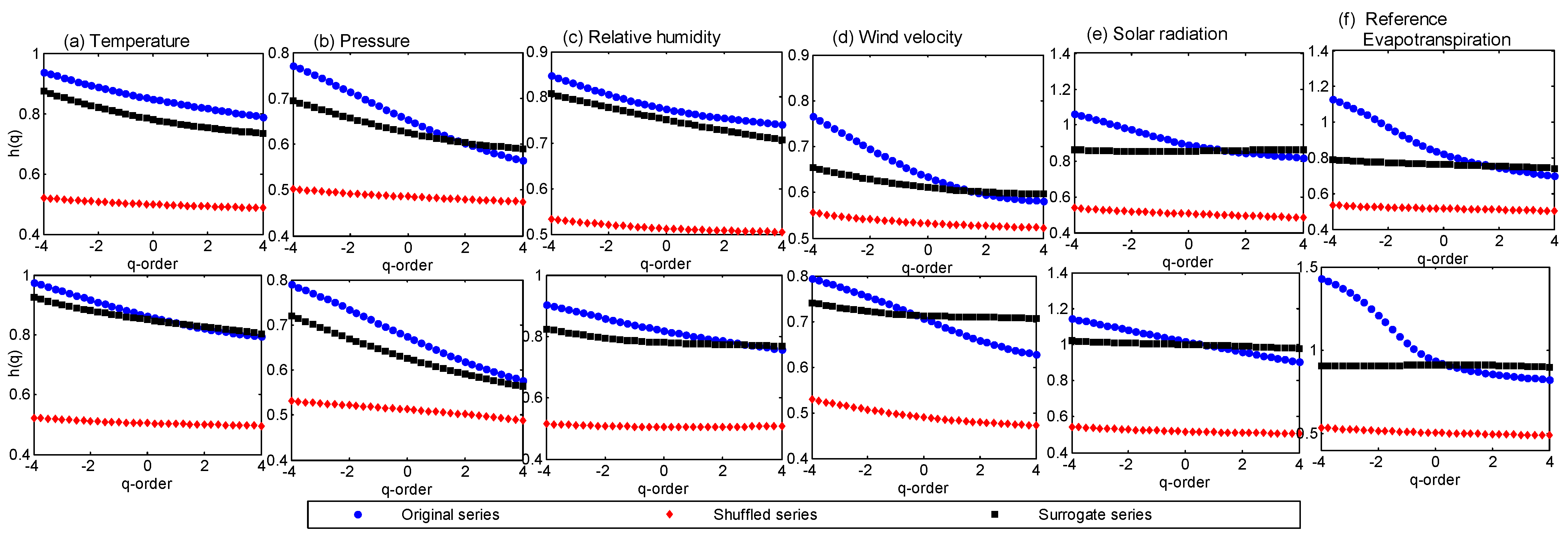
Determining the reason for multifractality is one of the important steps in multifractal studies. Two of the major reasons behind multifractality are (i) long-range correlations and (ii) the fatness (spreadness) of the probability density function (PDF). In this work, the shuffling processes were followed to find the origins of the multifractality. The shuffling process destroys any long-range correlation in the series but will retain the same probability distribution. To quantify the effect of the broadness of the PDF, a surrogate (SU) series developed from the original series is used. If the multifractal character is due to a correlation property, the h(q) of the shuffled (SH) series will be reduced to 0.5. If it is due to the spreadness of the PDF, the h(q) obtained for the surrogate series will show q-independency [63]. If both the long-range temporal correlations and broadness of the PDFs are leading to multifractality, both the SH and SU series will show lower multifractal strength than the original series. The details of random shuffling and the steps for generating SU series by the iterative amplitude-adjusted Fourier transform (IAAFT) algorithm can be found in the literature [64]. The comparison of the GHE plots of the original, SH, and SU series will help to find the origins of the multifractal behavior. The GHE plots of the original, SH, and SU series of all datasets of the Tabriz and Urmia stations are presented in Figure 8.
Overall, from Figure 8, it is noted that, for all variables, there is an overall reduction in h(q) values of the SH and SU series, which implies that the multifractal behavior can be attributed to both the long-range correlations and fatness of the PDF. It is noticed that multifractality is not fully destroyed by the SU scheme. Also, the shuffling operation has reduced the GHE values to close to 0.5, exhibiting the dominant role of the temporal correlation in the multifractality of the series. The statistics of GHE values of the original, SR, and SU series, along with the ∆h(q) values, are presented in Table 5.Table 5 shows that the H values of the shuffled series have been brought down to a value close to 0.5 with a small SD (<0.03). Thus, it can be concluded that the multifractal behaviors of the different series are dominated by temporal correlations.

4.3. MEMD-MFDFA Approach for Fractality Detection

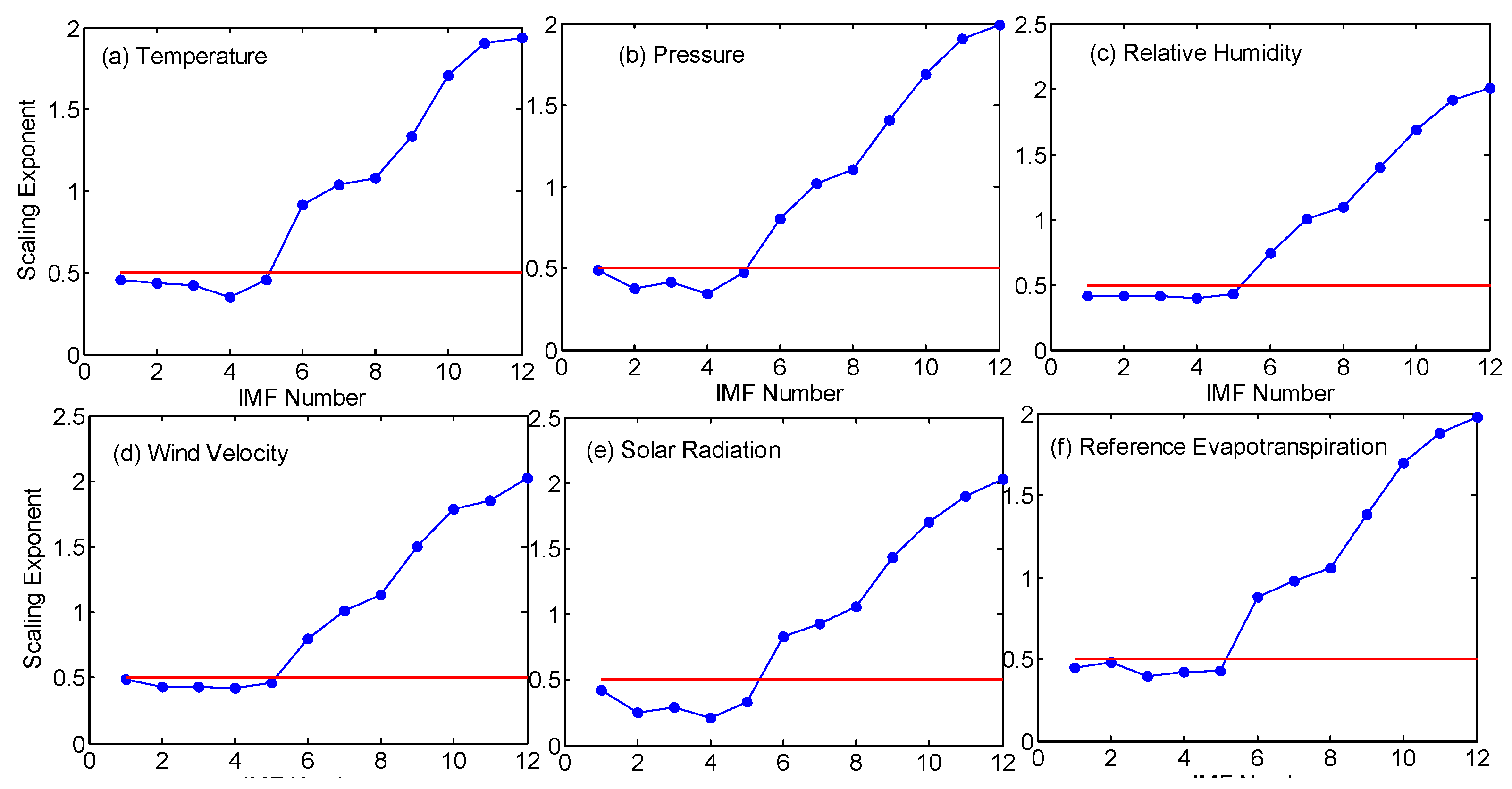
The proposed MEMD-MFDFA framework presented in Section 3.4 was invoked for time-series reconstruction for eliminating the nondominated (short memory modes) along with the Gaussian white noise expected in the high-frequency modes. The MEMD algorithm was applied to the multivariate dataset comprising six variables including evapotranspiration. The MEMD parameters of maximum threshold, minimum threshold, and fraction of decomposition were set as 0.75, 0.075, and 0.5, respectively, considering 64 direction vectors and following the guidelines given in past studies [49,50,51,65]. The decomposition resulted in 11 IMFs and one final residue for all six-time series. Subsequently, the MFDFA of each mode of each variable was performed, and the scaling exponent (value for q = 2) was extracted. The threshold value of the scaling exponent was fixed at 0.5, considering the classic categorization of long/short memory persistence of a time series [15]. The modes withvalues of scaling exponents falling below 0.5 were considered to be short memory and, therefore, were eliminated during the reconstruction process. The values of the scaling exponents of the rotatory modes of the different time series for the Tabriz and Urmia stations are presented in Figure 9 and Figure 10, respectively. For all the time series of Urmia station, the first five modes were found to be of short memory and were not considered for reconstruction. Among the different time series of Tabriz station, the temperature and ETo series for the first five modes were found to be of short memory, while for relative humidity and solar radiation, the first six modes were found to be of short memory. For the time series of pressure, the first four modes were found to be of short memory, while for the wind velocity time series of Tabriz station, modes 2 to 5 were found to be short memory. After eliminating the modes of short memory persistence, each time series was reconstructed and MFDFA was performed. The results of MFDFA for the reconstructed time series are presented in Table 6.
A comparison of the multifractal properties of the original series and reconstructed series (Table 2 and Table 4) show that the persistence and predictability of the different variables increased after de-noising and reconstruction.

4.4. MFCCA of Meteorological Variables with Reference Evapotranspiration

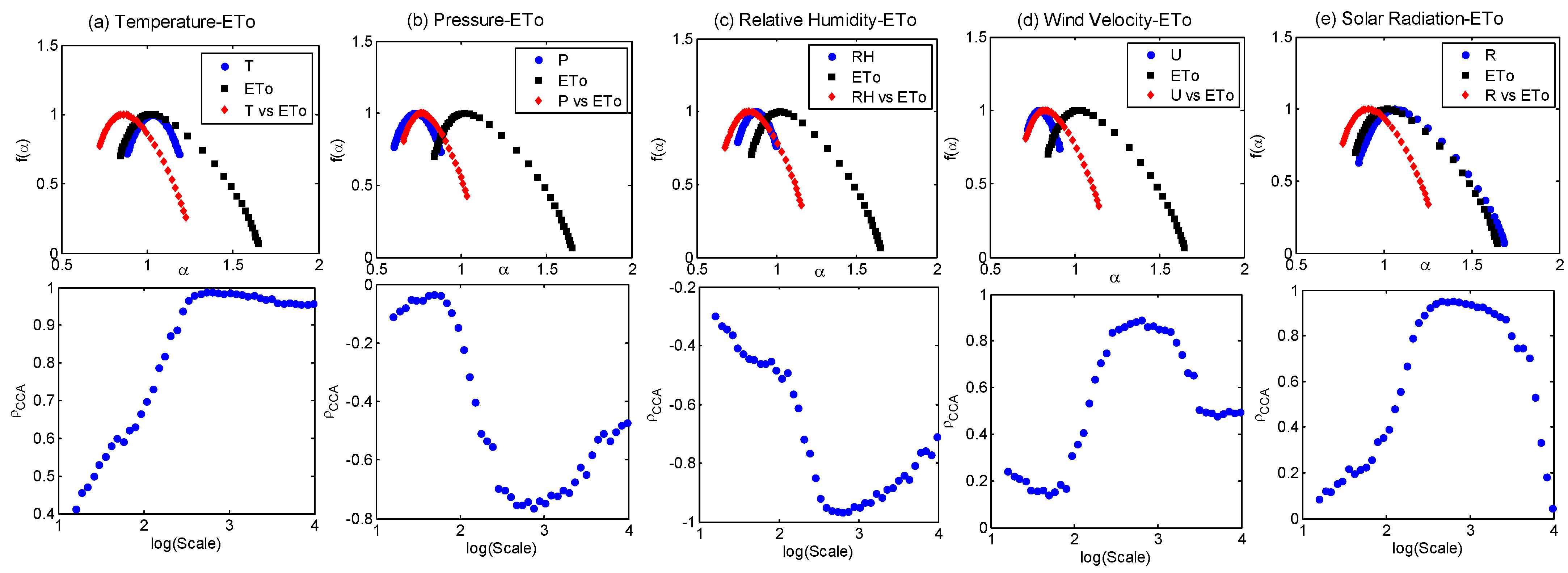
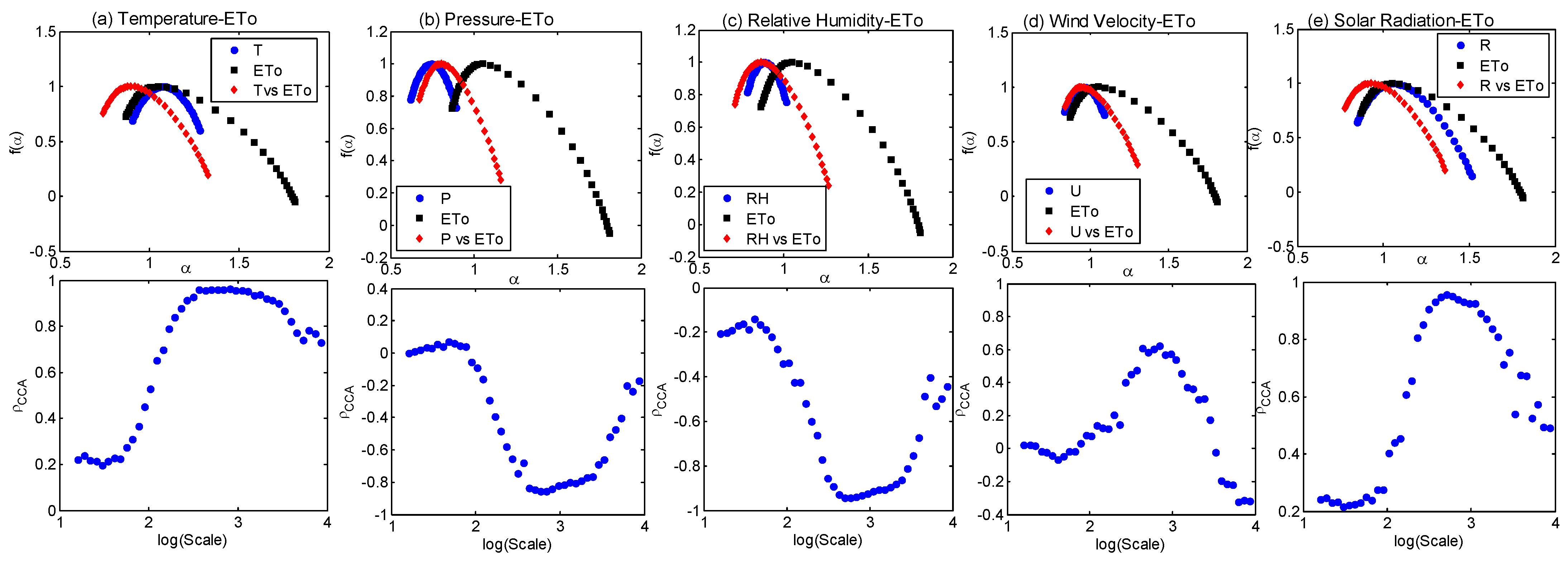
The MFCCA algorithm was then employed for finding the relationship between the different reconstructed meteorological variables with the ETo of both stations. The persistence of individual series, joint persistence, correlations at different scales, and multifractal spectra were determined for each case. The multifractal spectra and correlation plots of different pairs of variables (such as T-ETo, P-ETo, RH-ETo, U-ETo, and SR-ETo) for Tabriz station are presented in Figure 11, and the same for Urmia station are presented in Figure 12.
From Figure 11 and Figure 12, it is noticed that the shape of the multifractal spectra of different links are different for the two stations, while the spectra of the solar radiation and ETo of Tabriz station shows good similarity. However, the patterns of correlations for different links display similarity, even though the magnitudes of correlation differ. At all-time scales, the association of T, U, and SR with ETo are positive, while RH-ETo correlations are negative for both stations. It may be noted that P-ETo association for Tabriz station is negative at all time scales, while at some intra-annual scales, the association is weakly positive for Urmia station. Thus, MFCCA is successful in capturing such scale-dependent changes in the nature of the associations between different candidate hydro-climatic variables with ETo.
The cross-correlation coefficient (indicated as ρCCA in this paper) corresponding to 90 days is termed a seasonal cross-correlation coefficient and that corresponding to 365 days is termed an annual cross-correlation coefficient. The seasonal, annual, and overall correlations, along with the scaling exponent, spectral width (W), and R for different variables with ETo, are provided in Table 7.
From Table 7, it is noted that the combined scaling exponent (λxy) is nearly half of the scaling exponent (λx and λy) of the individual series. This is in agreement with the universal property on the persistence of time series by DCCA, proven by the researchers considering the sunspot–streamflow linkages. The seasonal and annual correlations with ETo were found to be positive for all variables except RH and P. In all links, the seasonal scale correlations were weak, while the annual scale correlations were found to be strong at both stations. The strongest annual scale correlations and overall correlations were noted in the SR-ETo link and T-ETo link, which is a quite anticipated result on considering the climatology of northwestern Iran. High multifractality was noted in the ETo series of both stations (spectral widths of 0.809 and 0.942 for Tabriz and Urmia, respectively). The multifractal spectra obtained for all combinations were right skewed, which was also indicated by the negative value of the asymmetric index. This implies that the extreme events play a prominent role in the temporal structure of the time series [27], indicating the high probability of low fluctuations. This study performed the multifractal analysis of daily reference ETo time series along with relevant meteorological variables affecting the process of evapotranspiration. This study was performed for the two stations of Tabriz and Urmia in northwestern Iran. The climatic processes of the region are controlled by the elevation and presence of Lake Urmia, along with the large-scale global climatic oscillations [32]. Thus, the scale-dependent relation of the meteorological variables of the region with ETo are controlled by these factors. Lake–atmosphere interactions create a complex coupled system, in which feedback currents between them can shape and modify the local/global climate conditions on Earth. As a hypersaline lake, Lake Urmia has impacts on its local atmosphere (also on the global climate in the largescale), of which the most important ones can be mentioned: like other great lakes, Lake Urmia (a) serves as a natural modulator of temperature during the seasons, resulting in cooler summers and warmer winters, (b) contributes to cloud formation, which helps adjust the Earth’s radiation equilibrium and leads to a series of intricate feedback mechanisms in atmospheric circulation, ultimately increasing precipitation and snowfall in the region, (c) reduces, by increasing the cloud cover, the incoming atmospheric radiation to the Earth’s surface, and (d) plays a significant role in wind formation by establishing a temperature gradient (the area surrounding a lake is consistently warmer than the lake itself, as water reflects most of the solar radiation back into the atmosphere, while land surfaces absorb more atmospheric radiation). In addition (e), as the water level drops, it results in a decrease in the local relative humidity and the lake breezes, as well as an increase in the temperature of and evaporation from the surrounding terrain, leading to salty sandstorms. The presence of airborne dust, including in salt and dust storms, poses risks of salinity for agriculture, adverse weather conditions for human life, and atmospheric dimming. Dimmed weather reduces incoming radiation and acts in a manner comparable to the greenhouse effect [66,67,68,69,70,71,72].
Researchers in the region are conducting in-depth studies on hydroclimatic issues. One specific task in this context is to determine which province (left or right) contributes more to the problem from both natural and anthropogenic perspectives. The interactions among the various parameters may have played a role in the fluctuation and nonlinear dynamic characteristics of the climatic variables and ETo of the region. This made differences and increased complexity, which is more evident in the series involving wind speed and surface pressure at Urmia station. These insights into the nonlinear dynamic patterns are considered valuable for enhancing the modeling of ETo and, consequently, for improving irrigation-water management. Furthermore, the recent changes in hydro-climatic extremes may be affecting the data characteristics, and to study their impact on fractality, it is recommended that more recent and extended datasets be utilized. Employing datasets covering a longer time span can aid in capturing the impact of evolving climate conditions on the ETo in any region, given that the methodology presented is applicable across different contexts.
The differences in multifractal properties may provide useful insights for developing prediction models of ETo, which are expected to display improved accuracy. The proposed MEMD-MFDFA framework could be used as a potential tool for signal reconstruction, and the knowledge of short or long memory persistence can be useful for improving the predictability of the series. The mutual association of different reconstructed meteorological variables with evapotranspiration was examined in a multifractal perspective through the MFCCA, a recently proposed sign-preserved variant in the family of cross-correlation algorithms. However, more experiments need to be solicited using the methods used in the study by considering long and continuous hydro-meteorological datasets of different climatic conditions. The knowledge gained from the study is to be extended for the prediction of ETo or related variables, integrating with the potential of hybrid machine learning or multifractal algorithms, in which, first, a decomposition-based data preprocessing can be undertaken for capturing scale-based associations. Subsequently, the scale-dependent modeling can be followed, and integration can be undertaken using machine learning methods or multifractal models [52]. Also, the presented MEMD framework has potential not only as a reconstruction tool but also opens the scope for performing scale-dependent multifractal modeling, and studies in these directions are in the pipeline.

5. Conclusions

This study investigated the multifractal characteristics of hydro-meteorological datasets of the Tabriz and Urmia stations of northwestern Iran using the MFDFA and MFCCA methods. MFDFA analysis showed that the daily reference evapotranspiration (ETo) and five other meteorological variables (temperature, pressure, relative humidity, wind velocity, and solar radiation) of both stations have multifractality and long memory persistence. The ETo time series of both stations exhibited the highest multifractality, while pressure and wind velocity exhibited the lowest persistence. The proposed MEMD-MFDFA coupled framework is a promising approach for reconstructing a hydro-meteorological time series. MFDFA analysis of the reconstructed signals highlighted an increase in persistence and multifractality behaviors compared to the original time series. The knowledge on short or long memory persistence gathered from the proposed framework can be used for improving the predictability of the series. The application of the MFCCA method could capture the scale-dependent association of different meteorological parameters with ETo. It was found that the joint persistence is nearly half of the persistence of the individual time series, which reinforced the universal property in the multifractal cross-correlation studies. The seasonal and annual cross-correlation properties displayed diversity in the strengths of different pair-wise combinations of cross-correlation analysis, but they displayed similar patterns for both stations. The knowledge gained from the study is helpful for developing decomposition-aided hybrid modeling frameworks for ETo prediction, in which MEMD can be used as a decomposition paradigm, and multifractal models can be used for the predication of its components at different scales.

Author Contributions

Conceptualization, A.S. (Adarsh Sankaran) and T.P.; methodology, A.S. (Adarsh Sankaran) and T.P.; software, A.S. (Adarsh Sankaran); formal analysis, S.V. and A.S. (Aayisha Salim); investigation, S.V. and A.S. (Aayisha Salim); data curation, V.N.; writing—original draft preparation, A.S. (Adarsh Sankaran); writing—review and editing, A.S. (Adarsh Sankaran), T.P. and V.N.; visualization, S.V. and A.S. (Aayisha Salim); supervision, A.S. (Adarsh Sankaran) and T.P. All authors have read and agreed to the published version of the manuscript.

Funding

This research received no external funding.

Institutional Review Board Statement

Not applicable.

Informed Consent Statement

Not applicable.

Data Availability Statement

Data cannot be shared in public platforms. The data used in the study will be transferred for academic purposes upon genuine requests to authors after receiving permission from the Iranian meteorological agencies.

Conflicts of Interest

The authors declare no conflict of interest.

Appendix A

The schematic view of the MFDFA algorithm is provided in Figure A1.
The Hurst exponent (h(q = 2)) may decipher the persistence of the signal, while the deduced results, such as the Renyi exponent (τ(q)) and multifractal spectrum, may help to decode the multifractal behavior of the signal. The multifractal exponents can be computed as [17]:
τ ( q ) = q h ( q ) 1
α = d τ ( q ) d q
and
f ( α ) = q α τ ( q )
The f(α) vs. α plot is called the multifractal spectrum and the support of the spectrum.
( Δ α = α max α min ) shows the multifractal strength of the time series. The wider the spectrum, the higher will be the strength of the multifractality [18]. For a multifractal signal, the geometry of the plot will be a downward parabola that converges to a point for a monofractal series. The asymmetry index (R) is deduced from the singularity spectrum to indicate the fluctuation frequency:
R = Δ α L Δ α R Δ α L + Δ α R
where Δ α R = α max α 0 and Δ α L = α 0 α min are the widths of the right and left limbs of the spectrum, respectively, and α 0 is the singularity exponent for q = 0 (known as the Holder exponent), R [ 1 1 ] , and the positive value of this index represents the right-hand deviation of the multifractal spectrum, indicating a high probability of high fluctuations. The negative value of R shows that the series is characterized by localized low fluctuations.
Figure A1. Procedure of MFDFA.
Atmosphere 14 01219 g0a1

References

  1. Allen, R.G.; Pereira, L.S.; Raes, D.; Smith, M. Crop evapotranspiration-Guidelines for computing crop water requirements-FAO Irrigation and drainage paper 56. Fao Rome 1998, 300, D05109. [Google Scholar]
  2. Adarsh, S.; Nityanjaly, L.J.; Sarang, R.; Pham, Q.B.; Ali, M.; Nandhineekrishna, P. Multifractal Characterization and Cross correlations of Reference Evapotranspiration Time Series of India. Eur. Phys. J. Spec. Top. 2021, 230, 3845–3859. [Google Scholar] [CrossRef]
  3. Goyal, P.; Kumar, S.; Sharda, R. A review of the Artificial Intelligence (AI) based techniques for estimating reference evapotranspiration: Current trends and future perspectives. Comput. Electron. Agric. 2023, 209, 107836. [Google Scholar] [CrossRef]
  4. Hurst, H.E. Long-term storage capacity of reservoirs. Trans. Am. Soc. Civ. Eng. 1951, 116, 770–808. [Google Scholar] [CrossRef]
  5. Mandelbrot, B. The Fractal Geometry of Nature; WH Freeman Publishers: New York, NY, USA, 1982. [Google Scholar]
  6. Pandey, G.; Lovejoy, S.; Schertzer, D. Multifractal analysis of daily river flows including extremes for basins five to two million square kilometers, one day to 75 years. J. Hydrol. 1998, 208, 62–81. [Google Scholar] [CrossRef]
  7. Kantelhardt, J.W.; Rybski, D.; Zschiegner, S.A.; Braun, P.; Koscielny-Bunde, E.; Livina, V.; Havlin, S.; Bunde, A. Multifractality of river runoff and precipitation: Comparison of fluctuation analysis and wavelet methods. Phys. A Stat. Mech. Its Appl. 2003, 330, 240–245. [Google Scholar] [CrossRef] [Green Version]
  8. Huang, Y.; Schmitt, F.G.; Lu, Z.; Liu, Y. Analysis of daily river flow fluctuations using empirical mode decomposition and arbitrary order Hilbert spectral analysis. J. Hydrol. 2009, 373, 103–111. [Google Scholar] [CrossRef] [Green Version]
  9. Schmitt, F.; Schertzer, D.; Lovejoy, S. Multifractal analysis of foreign exchange data. Appl. Stoch. Models Data Anal. 1999, 15, 29–53. [Google Scholar] [CrossRef]
  10. Plocoste, T.; Calif, R.; Jacoby-Koaly, S. Temporal multiscaling characteristics of particulate matter PM10 and ground-level ozone O3 concentrations in Caribbean region. Atmos. Environ. 2017, 169, 22–35. [Google Scholar] [CrossRef]
  11. Carmona-Cabezas, R.; Ariza-Villaverde, A.B.; de Ravé, E.G.; Jiménez-Hornero, F.J. Visibility graphs of ground-level ozone time series: A multifractal analysis. Sci. Total Environ. 2021, 661, 138–147. [Google Scholar] [CrossRef]
  12. Plocoste, T.; Carmona-Cabezas, R.; Jiménez-Hornero, F.J.; de Ravé, E.G.; Calif, R. Multifractal characterisation of particulate matter (PM10) time series in the Caribbean basin using visibility graphs. Atmos. Pollut. Res. 2021, 12, 100–110. [Google Scholar] [CrossRef]
  13. Peng, C.K.; Buldyrev, S.V.; Havlin, S.; Simons, M.; Stanley, H.E.; Goldberger, A.L. Mosaic organization of DNA nucleotides. Phys. Rev. E 1994, 49, 1685. [Google Scholar] [CrossRef] [Green Version]
  14. Kantelhardt, J.W.; Zschiegner, S.A.; Koscielny-Bunde, E.; Havlin, S.; Bunde, A.; Stanley, H.E. Multifractal detrended fluctuation analysis of non-stationary time series. Phys. A Stat. Mech. Its Appl. 2002, 316, 87–114. [Google Scholar] [CrossRef] [Green Version]
  15. Kantelhardt, J.W.; Koscielny-Bunde, E.; Rybski, D.; Braun, P.; Bunde, A.; Havlin, S. Long-term persistence and multifractality of precipitation and river runoff records. J. Geophys. Res. Atmos. 2006, 111. [Google Scholar] [CrossRef]
  16. Koscielny-Bunde, E.; Kantelhart, J.W.; Braun, P.; Bunde, A.; Havlin, S. Long-term persistence and multifractality of river runoff records: Detrended fluctuation studies. J. Hydrol. 2006, 322, 120–137. [Google Scholar] [CrossRef] [Green Version]
  17. Li, E.; Mu, X.; Zhao, G.; Gao, P. Multifractal detrended fluctuation analysis of streamflow in the Yellow River Basin, China. Water 2015, 7, 1670–1686. [Google Scholar] [CrossRef] [Green Version]
  18. Hou, W.; Feng, G.; Yan, P.; Li, S. Multifractal analysis of the drought area in seven large regions of China from 1961 to 2012. Meteorol. Atmos. Phys. 2018, 130, 459–471. [Google Scholar] [CrossRef] [Green Version]
  19. Adarsh, S.; Dharan, D.S.; Nandhu, A.R.; Anand Vishnu, B.; Mohan, V.K.; Watorek, M. Multifractal Description of Streamflow and Suspended Sediment Concentration Data from Indian River Basins. Acta Geophys. 2020, 68, 519–535. [Google Scholar] [CrossRef] [Green Version]
  20. Adarsh, S.; Krzyszczak, J.; Baranowski, P.; Archana, D.S.; Nandhinee krishna, P.; Nityanjaly, L.J.; Vandana, T.; Ali, M. Multifractal Cross Correlation Analysis of Agro-Meteorological Datasets (Including Reference Evapotranspiration) of California. Atmosphere 2020, 11, 1116. [Google Scholar] [CrossRef]
  21. Martínez, J.L.M.; Segovia-Domínguez, I.; Rodríguez, I.Q.; Horta-Rangel, F.A.; Sosa-Gómez, G. A modified Multifractal Detrended Fluctuation Analysis (MFDFA) approach for multifractal analysis of precipitation. Phys. A Stat. Mech. Its Appl. 2021, 565, 125611. [Google Scholar] [CrossRef]
  22. Zhan, C.; Liang, C.; Zhao, L.; Jiang, S.; Niu, K.; Zhang, Y. Multifractal characteristics of multiscale drought in the Yellow River Basin, China. Phys. A Stat. Mech. Its Appl. 2023, 609, 128305. [Google Scholar] [CrossRef]
  23. Lin, G.; Chen, X.; Fu, Z. Temporal–spatial diversities of long-range correlation for relative humidity over China. Phys. A Stat. Mech. Its Appl. 2007, 383, 585–594. [Google Scholar] [CrossRef]
  24. Yuan, N.; Fu, Z.; Mao, J. Different multi-fractal behaviors of diurnal temperature range over the north and the south of China. Theor. Appl. Climatol. 2013, 112, 673–682. [Google Scholar] [CrossRef]
  25. Burgueño, A.; Lana, X.; Serra, C.; Martínez, M.D. Daily extreme temperature multifractals in Catalonia (NESpain). Phys. Lett. A 2014, 378, 874–885. [Google Scholar] [CrossRef]
  26. Kalamaras, N.; Philippopoulos, K.; Deligiorgi, D.; Tzanis, C.G.; Karvounis, G. Multifractal scaling properties of daily air temperature time series. Chaos Solitons Fractals 2017, 98, 38–43. [Google Scholar] [CrossRef]
  27. Krzyszczak, J.; Baranowski, P.; Zubik, M.; Kazandjiev, V.; Georgieva, V.; Sławiński, C.; Siwek, K.; Kozyra, J.; Nieróbca, A. Multifractal characterization and comparison of meteorological time series from two climatic zones. Theor. Appl. Climatol. 2019, 137, 1811–1824. [Google Scholar] [CrossRef] [Green Version]
  28. Plocoste, T.; Pavón-Domínguez, P. Multifractal detrended cross-correlation analysis of wind speed and solar radiation. Chaos Interdiscip. J. Nonlinear Sci. 2020, 30, 113109. [Google Scholar] [CrossRef]
  29. Baranowski, P.; Krzyszczak, J.; Slawinski, C.; Hoffmann, H.; Kozyra, J.; Nieróbca, A.; Siwek, K.; Gluza, A. Multifractal analysis of meteorological time series to assess climate impacts. Clim. Res. 2015, 65, 39–52. [Google Scholar] [CrossRef] [Green Version]
  30. Nourani, V.; Elkiran, G.; Abdullah, J. Multi-station artificial intelligence-based ensemble modeling of reference evapotranspiration using pan evaporation measurements. J. Hydrol. 2019, 577, 123958. [Google Scholar] [CrossRef]
  31. Nourani, V.; Elkiran, G.; Abdullah, J. Multi-step ahead modeling of reference evapotranspiration using a multi-model approach. J. Hydrol. 2020, 581, 124434. [Google Scholar] [CrossRef]
  32. Sreedevi, V.; Adarsh, S.; Nourani, V. Multiscale coherence analysis of reference evapotranspiration of north-western Iran using wavelet transform. J. Water Clim. Chang. 2022, 13, 505–521. [Google Scholar] [CrossRef]
  33. Suman, A.; Archana, D.S.; Nayak, A.K.; Adarsh, S.; Biswal, B. Unveiling the Climatic origin of Streamflow persistence through Multifractal Analysis of Hydrometeorological datasets of India. Hydrol. Sci. J. 2023, 68, 290–306. [Google Scholar] [CrossRef]
  34. Ariza-Villaverde, A.B.; Pavón-Domínguez, P.; Carmona-Cabezas, R.; Gutierrez de Rave, E.; Jimenez-Honero, F.J. Joint multifractal analysis of air temperature, relative humidity and reference evapotranspiration in the middle zone of the Guadalquivir river valley. Agric. For. Meteorol. 2019, 278, 107657. [Google Scholar] [CrossRef]
  35. Cun, Z.; Liang, C.; Zhao, L.; Zhang, Y.; Cheng, L.; Jiang, S.; Xing, L. Multifractal characteristics analysis of daily reference evapotranspiration in different climate zones of China. Phys. A Stat. Mech. Its Appl. 2021, 583, 126273. [Google Scholar] [CrossRef]
  36. Gómez-Gómez, J.; Ariza-Villaverde, A.B.; Gutiérrez de Ravé, E.; Jiménez-Hornero, F.J. Relationships between Reference Evapotranspiration and Meteorological Variables in the Middle Zone of the Guadalquivir River Valley Explained by Multifractal Detrended Cross-Correlation Analysis. Fractal Fract. 2023, 7, 54. [Google Scholar] [CrossRef]
  37. Nourani, V.; Fard, M.S. Sensitivity analysis of the artificial neural network outputs in simulation of the evaporation process at different climatologic regimes. Adv. Eng. Softw. 2016, 47, 127–146. [Google Scholar] [CrossRef]
  38. Podobnik, B.; Stanley, H.E. Detrended cross-correlation analysis: A new method for analyzing two nonstationary time series. Phys. Rev. Lett. 2008, 100, 084102. [Google Scholar] [CrossRef] [Green Version]
  39. Zhou, W.-X. Multifractal detrended cross-correlation analysis for two non-stationary signals. Phys. Rev. E 2008, 77, 066211. [Google Scholar] [CrossRef] [Green Version]
  40. Jiang, Z.-Q.; Zhou, W.-X. Multifractal detrending moving-average cross-correlation analysis. Phys. Rev. E 2011, 84, 016106. [Google Scholar] [CrossRef] [Green Version]
  41. Oświȩcimka, P.; Drożdż, S.; Forczek, M.; Jadach, S.; Kwapień, J. Detrended cross-correlation analysis consistently extended to multifractality. Phys. Rev. E 2014, 89, 023305. [Google Scholar] [CrossRef] [PubMed] [Green Version]
  42. Hajian, S.; Movahed, M.S. Multifractal detrended cross-correlation analysis of sunspot numbers and river flow fluctuations. Phys. A Stat. Mech. Its Appl. 2010, 389, 4942–4954. [Google Scholar] [CrossRef] [Green Version]
  43. Dey, P.; Mujumdar, P.P. Multiscale evolution of persistence of rainfall and streamflow. Adv. Water Resour. 2018, 121, 285–303. [Google Scholar] [CrossRef]
  44. Maghyereh, A.; Abdoh, H.; Wątorek, M. The impact of COVID-19 pandemic on the dynamic correlations between gold and U.S. equities: Evidence from multifractal cross-correlation analysis. Qual. Quant. 2023, 57, 1889–1903. [Google Scholar] [CrossRef]
  45. Kwapień, J.; Oświęcimka, P.; Drożdż, S. Detrended fluctuation analysis made flexible to detect range of cross-correlated fluctuations. Phys. Rev. E 2015, 92, 052815. [Google Scholar] [CrossRef] [Green Version]
  46. Brito, A.A.; Santos, F.R.; de Castro, A.P.N.; da Cunha Lima, A.T.; Zebende, G.F.; da Cunha Lima, I.C. Cross-correlation in a turbulent flow: Analysis of the velocity field using the σ DCCA coefficient. Eur. Lett. 2018, 123, 20011. [Google Scholar] [CrossRef]
  47. Wątorek, M.; Drożdż, S.; Kwapień, J.; Minati, L.; Oświȩcimka, P.; Stanuszek, M. Multiscale characteristics of the emerging global cryptocurrency market. Phys. Rep. 2021, 901, 1–82. [Google Scholar] [CrossRef]
  48. Wątorek, M.; Drożdż, S.; Oświęcimka, P.; Stanuszek, M. Multifractal cross-correlations between the world oil and other financial markets in 2012–2017. Energy Econ. 2019, 81, 874–885. [Google Scholar] [CrossRef] [Green Version]
  49. Rehman, N.; Mandic, D.P. Multivariate empirical mode decomposition. Proc. R. Soc. A 2011, 466, 1291–1302. [Google Scholar] [CrossRef]
  50. Hu, W.; Si, B.-C. Soil water prediction based on its scale-specific control using multivariate empirical mode decomposition. Geoderma 2013, 193–194, 180–188. [Google Scholar] [CrossRef]
  51. Huang, G.; Su, Y.; Kareem, A.; Liao, H. Time-frequency analysis of non-stationary process based on multivariate empirical mode decomposition. J. Eng. Mech. 2016, 142, 04015065. [Google Scholar] [CrossRef]
  52. Adarsh, S.; Sulaiman, S.; Murshida, K.K.; Nooramol, P. Scale-dependent prediction of reference evapotranspiration based on Multivariate Empirical Mode Decomposition. Ain Shams Eng. J. 2018, 9, 1839–1848. [Google Scholar] [CrossRef]
  53. Adarsh, S.; Janga Reddy, M. Multiscale characterization and prediction of reservoir inflows using MEMD-SLR Coupled Approach. J. Hydrol. Eng. 2019, 24, 04018059. [Google Scholar] [CrossRef]
  54. Ali, M.; Deo, R.C.; Maraseni, T.; Downs, N.J. Improving SPI-derived drought forecasts incorporating synoptic-scale climate indices in multi-phase multivariate empirical mode decomposition model hybridized with simulated annealing and kernel ridge regression algorithms. J. Hydrol. 2019, 576, 164–184. [Google Scholar] [CrossRef]
  55. Agana, N.A.; Homaifar, A. EMD-based predictive deep belief network for time series prediction: An application to drought forecasting. Hydrology 2018, 5, 18. [Google Scholar] [CrossRef] [Green Version]
  56. Cleveland, R.B.; Cleveland, W.S. STL: A Seasonal-Trend Decomposition Procedure Based on Loess. J. Off. Stat. 1990, 6, 3–33. [Google Scholar]
  57. Drożdż, S.; Minati, L.; Oświȩcimka, P.; Stanuszek, M.; Wątorek, M. Signatures of the Crypto-Currency Market Decoupling from the Forex. Future Internet 2019, 11, 154. [Google Scholar] [CrossRef] [Green Version]
  58. Chandrasekaran, C.; Poomalai, P.; Saminathan, B.; Suthanthiravel, S.; Sundaram, K.; Hakkim, F.F.A. An investigation on the relationship between the Hurst exponent and the predictability of a rainfall time series. Meteorol. Appl. 2019, 16, 511–519. [Google Scholar] [CrossRef] [Green Version]
  59. Orth, R.; Seneviratne, S.I. Predictability of soil moisture and streamflow on subseasonal timescales: A case study. J. Geophys. Res. Atmos. 2013, 118, 963–979. [Google Scholar] [CrossRef]
  60. Rangarajan, G.; Sant, D.A. A climate predictability index and its applications. Geophys. Res. Lett. 1997, 24, 1239–1242. [Google Scholar] [CrossRef]
  61. Peyghami, M.R.; Khanduzi, R. Predictability and forecasting automotive price based on a hybrid train algorithm of MLP neural network. Neural Comput. Appl. 2012, 21, 125–132. [Google Scholar] [CrossRef]
  62. Khalili, N.; Khodashenas, S.R.; Davary, K.; Baygi, M.M.; Karimaldini, F. Prediction of rainfall using artificial neural networks for synoptic station of Mashhad: A case study. Arab. J. Geosc. 2016, 9, 624. [Google Scholar] [CrossRef]
  63. Movahed, M.S.; Jafari, G.R.; Ghasemi, F.; Rahvar, S.; Tabar, M.R.R. Multifractal detrended fluctuation analysis of sunspot time series. J. Stat. Mech. Theory Exp. 2006, 2006, P02003. [Google Scholar] [CrossRef] [Green Version]
  64. Keylock, C.J. Hypothesis testing for nonlinear phenomena in the geosciences using synthetic, surrogate data. Earth Space Sci. 2019, 6, 41–58. [Google Scholar] [CrossRef]
  65. Rilling, G.; Flandrin, P.; Goncalves, P. On empirical mode decomposition and its algorithms. In Proceedings of the IEEE-EURASIP Workshop on Nonlinear Signal and Image Processing NSIP-03, Grado, Italy, 8–11 June 2003; Volume 3, pp. 1–5. [Google Scholar]
  66. Gerken, T.; Biermann, T.; Babel, W.; Herzog, M.; Ma, Y.; Foken, T.; Graf, H.F. A modelling investigation into lake-breeze development and convection triggering in the Nam Co Lake basin, Tibetan Plateau. Theor. Appl. Climatol. 2014, 117, 149–167. [Google Scholar] [CrossRef]
  67. Sun, X.; Xie, L.; Semazzi, F.H.; Liu, B. A numerical investigationof the precipitation over Lake Victoria basin using a coupledatmosphere-lake limited-area model. Adv. Meteorol. 2014, 2014, 960924. [Google Scholar] [CrossRef] [Green Version]
  68. Dehghanipour, A.H.; Moshir Panahi, D.; Mousavi, H.; Kalantari, Z.; Tajrishy, M. Effects of Water Level Decline in Lake Urmia, Iran, on Local Climate Conditions. Water 2020, 12, 2153. [Google Scholar] [CrossRef]
  69. Nourani, V.; Tootoonchi, R.; Andaryani, S. Investigation of climate, land cover and lake level pattern changes and interactions using remotely sensed data and wavelet analysis. Ecol. Inform. 2021, 64, 101330. [Google Scholar] [CrossRef]
  70. Nourani, V.; Sayyah-Fard, M.; Kantoush, S.A.; Bharambe, K.P.; Sumi, T.; Saber, M. Optimization-based prediction uncertainty qualification of climatic parameters. J. Hydrometeorol. 2023. [Google Scholar] [CrossRef]
  71. Plocoste, T.; Calif, R.; Euphrasie-Clotilde, L.; Brute, F.N. Investigation of local correlations between particulate matter (PM10) and air temperature in the Caribbean basin using Ensemble Empirical Mode Decomposition. Atmos. Pollut. Res. 2020, 11, 1692–1704. [Google Scholar] [CrossRef]
  72. Plocoste, T.; Calif, R. Is there a causal relationship between Particulate Matter (PM10) and air Temperature data? An analysis based on the Liang–Kleeman information transfer theory. Atmos. Pollut. Res. 2021, 12, 101177. [Google Scholar] [CrossRef]
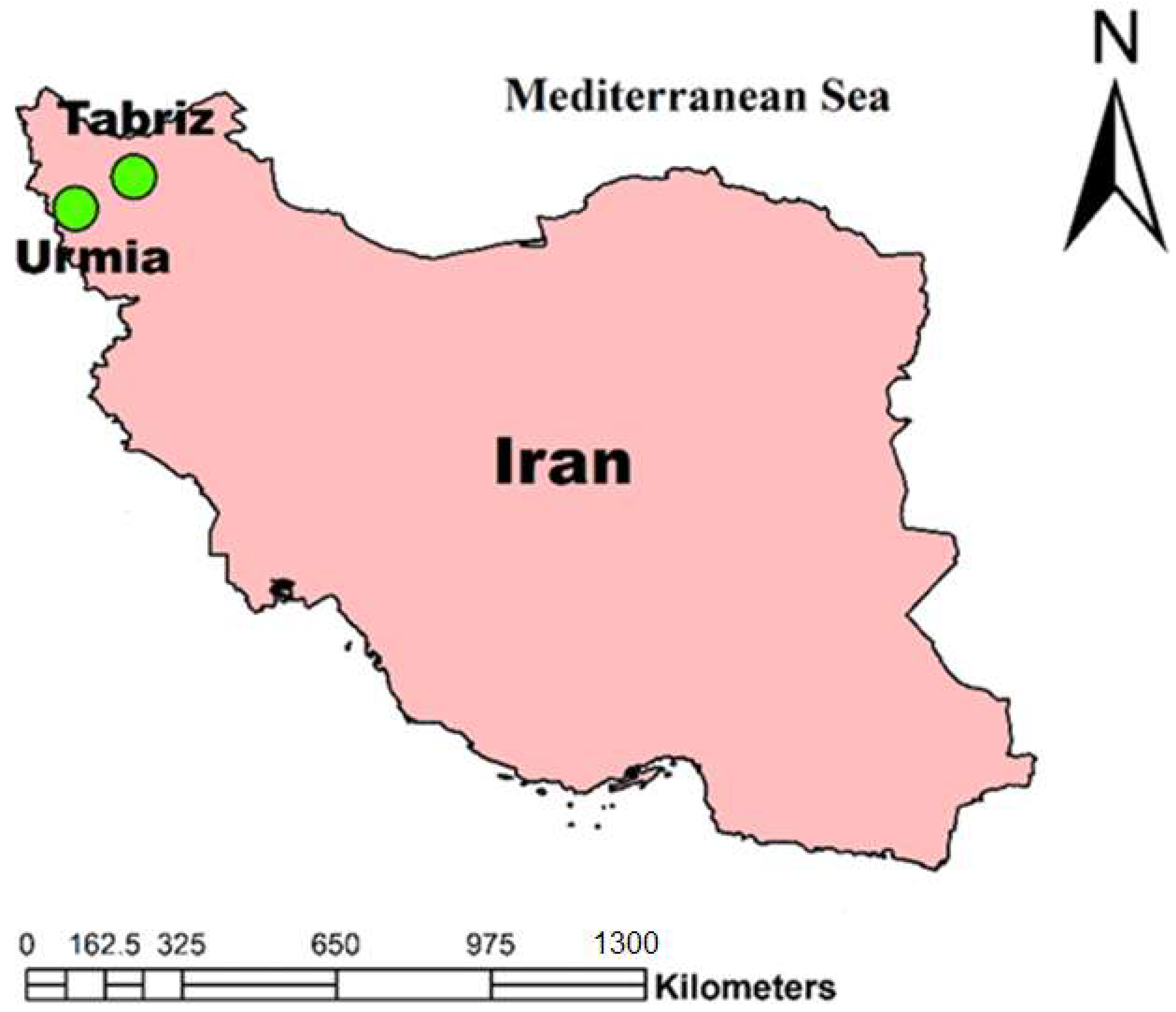
Figure 1. Locations of Tabriz and Urmia in northwestern Iran.
Atmosphere 14 01219 g001
Figure 2. Time-series plots of hydro-meteorological variables at Tabriz station for (a) temperature, (b) pressure, (c) relative humidity, (d) wind velocity, (e) solar radiation, and (f) reference evapotranspiration (ETo).
Atmosphere 14 01219 g002
Figure 3. Time-series plots of hydro-meteorological variables at Urmia station for (a) temperature, (b) pressure, (c) relative humidity, (d) wind velocity, (e) solar radiation, and (f) reference evapotranspiration (ETo).
Atmosphere 14 01219 g003
Figure 4. Flowchart of MEMD-MFDFA method for signal reconstruction.
Atmosphere 14 01219 g004
Figure 5. Fluctuation function plots of different variables at Tabriz station for (a) temperature, (b) pressure, (c) relative humidity, (d) wind velocity, (e) solar radiation, and (f) reference evapotranspiration.
Atmosphere 14 01219 g005
Figure 6. Fluctuation function plots of different variables at Urmia station for (a) temperature, (b) pressure, (c) relative humidity, (d) wind velocity, (e) solar radiation, and (f) reference evapotranspiration.
Atmosphere 14 01219 g006
Figure 7. Multifractal characteristics of hydro-meteorological variables at Tabriz and Urmia stations for (a) temperature, (b) pressure, (c) relative humidity, (d) wind velocity, (e) solar radiation, and (f) reference evapotranspiration. The upper panels show the GHE plots, middle panels show the Renyi exponent plots, and the lower panels show the singularity spectrum.
Atmosphere 14 01219 g007
Figure 8. Generalized Hurst exponentplots of original, SHand SU time series of different hydro-meteorological variables at Tabriz and Urmia stations for (a) temperature, (b) pressure, (c) relative humidity, (d) wind velocity, (e) solar radiation, and (f) reference evapotranspiration. The upper panels show the plots of Tabriz station, and the lower panels show the plots of Urmia station.
Atmosphere 14 01219 g008
Figure 9. Plots of scaling exponents (for q = 2) of the modes of different variables at Tabriz station for (a) temperature, (b) pressure, (c) relative humidity, (d) wind velocity, (e) solar radiation, and (f) reference evapotranspiration.
Atmosphere 14 01219 g009
Figure 10. Plots of scaling exponents of the modes of different variables at Urmia station for (a) temperature, (b) pressure, (c) relative humidity, (d) wind velocity, (e) solar radiation, and (f) reference evapotranspiration.
Atmosphere 14 01219 g010
Figure 11. Multifractal spectra and cross-correlation plots obtained by MFCCA of different links at Tabriz station for (a) temperature–ETo, (b) pressure–ETo, (c) relative humidity–ETo, (d) wind velocity–ETo, and (e) solar radiation–ETo.
Atmosphere 14 01219 g011
Figure 12. Multifractal spectra and cross-correlation plots obtained by MFCCA of different links at Urmia station for (a) temperature–ETo, (b) pressure–ETo, (c) relative humidity–ETo, (d) wind velocity–ETo, and (e) solar radiation–ETo.
Atmosphere 14 01219 g012
Table 1. Statistical properties of hydro-meteorological variables of the Tabriz and Urmia stations. SD and CV respectively show the standard deviation and the coefficient of variation.
StationVariableFromToStatistical Property
MaximumMinimumMeanSDCV (%)
TabrizTemperature (°C)1/6/199226/10/201833.20−15.00013.3410.3877.81
Pressure (kPa)1/6/199226/10/2018878.44850.95864.404.320.50
Relative Humidity (%)1/6/199226/10/201895.87510.550.5717.68334.96
Wind Velocity (ms−1)1/6/199226/10/20189.5000.003.3841.6047.28
Solar Radiation (kJ m−2)1/6/199226/10/2018347943.001698.0792.2246.65
Evapotranspiration (mm)1/6/199226/10/201821.20−0.1856.15984.8893579.37
UrmiaTemperature (°C)1/6/199210/11/201830.00−13.0011.889.4279.29
Pressure (kPa)1/6/199226/10/2018882.00853.24867.194.470.515
Relative Humidity (%)1/6/199226/10/201899.5020.1357.9915.6927.06
Wind Velocity (ms−1)1/6/199226/10/20187.630.002.131.1152.11
Solar Radiation (kJ m−2)1/6/199226/10/20183540.0016.001774.16805.3045.39
Evapotranspiration (mm)1/6/199226/10/201813.800.004.133.3982.08
Table 2. Multifractal properties of different hydro-meteorological variables of the Tabriz and Urmia stations.
StationVariableHWR∆f(α)∆h(q)α0
TabrizTemperature (T)0.8180.2980.2960.1920.1490.845
Pressure (P)0.6010.3660.2370.1700.2070.646
Relative Humidity (RH)0.7540.2130.4950.2390.1070.771
Wind Velocity (WV)0.6070.4300.3460.3180.2300.651
Solar Radiation (SR)0.8450.4380.4450.3400.2440.883
Reference Evapotranspiration (ET0)0.7460.7350.4870.6000.4300.810
UrmiaTemperature (T)0.8210.3310.3410.2310.1820.856
Pressure (P)0.6190.3740.1570.0970.2130.666
Relative Humidity (RH)0.7850.2760.2470.1370.1460.814
Wind Velocity (WV)0.6590.2740.1460.0750.1660.700
Solar Radiation (SR)0.9600.4510.0730.0300.2400.991
Reference Evapotranspiration (ET0)0.8570.9270.6860.8700.6070.919
Table 3. Fractal dimension and predictability index for the different variables.
StationVariableDPI
TabrizT1.1820.636
P1.3990.202
RH1.2460.508
WV1.3930.214
SR1.1550.690
ET01.2540.492
UrmiaT1.1790.642
P1.3810.238
RH1.2150.570
WV1.3410.318
SR1.0400.920
ET01.1430.714
Table 4. Persistence of the total time series and the different sub-series for all variables (CL: complete length; FH: first half; SH: second half; FQ: first quarter; SQ: second quarter; TQ: third quarter; FQ: fourth quarter; FRQ: first three quarter; LTQ: last three quarter).
StationVariableCLFHSHMHFQSQTQFRQFTQLTQ
TabrizT0.8180.8000.8670.8280.8560.7820.9040.8760.8130.829
P0.6010.6390.6440.6290.7200.6780.6820.6640.6170.608
RH0.7540.7170.8150.7850.7400.7360.8710.8150.7580.779
WV0.6070.6390.5820.5910.6220.5800.6050.5560.6430.573
SR0.8450.9080.8150.9080.8880.8780.8930.6900.8950.848
ET00.7460.7630.7680.7830.7430.7410.7970.7930.7600.769
UrmiaT0.8210.8040.8830.8440.8740.7980.9100.8890.8220.837
P0.6190.6430.6610.6380.7320.6500.7020.6830.6300.628
RH0.7850.7860.8260.8020.7970.7590.8430.8370.7970.808
WV0.6590.6240.7220.6100.6810.5340.6170.7500.6790.691
SR0.9600.9940.9670.9910.9220.9990.9900.8770.9960.977
ET00.8570.8600.8680.8680.8140.7820.8330.8500.8710.871
Table 5. Statistics of the generalized Hurst exponent of the original, SH, and SU series of the different datasets of the Tabriz and Urmia stations. SD is the standard deviation.
VariablePropertyTabriz StationUrmia Station
Original SeriesShuffled
Series
Surrogate
Series
Original
Series
Shuffled
Series
Surrogate
Series
TemperatureMean0.8560.5010.7900.8710.5060.855
SD0.0450.0100.0420.0570.0080.035
∆h(q)0.1490.0330.1400.1820.0270.121
PressureMean0.6590.4860.6310.6780.5110.632
SD0.0650.0080.0330.0670.0120.048
∆h(q)0.2070.0280.1050.2130.0420.157
Relative HumidityMean0.7820.5150.7530.8230.5070.786
SD0.0330.0080.0310.0450.0030.016
∆h(q)0.1070.0280.1000.1460.0080.056
Wind VelocityMean0.6490.5350.6161.0210.5200.999
SD0.0590.0100.0180.0730.0110.012
∆h(q)0.1840.0330.0580.2400.0370.041
Solar RadiationMean0.9120.5060.8561.0330.5070.907
SD0.0780.0160.0030.2100.0130.003
∆h(q)0.2440.0550.0000.6070.0470.010
Reference
Evapotranspiration
Mean0.8640.5170.7640.7080.4940.716
SD0.1380.0090.0130.0540.0170.010
∆h(q)0.4300.0330.0470.1660.0570.034
Table 6. Multifractal properties of reconstructed hydro-meteorological variables of Tabriz and Urmia stations.
StationVariableHWR∆f(α)∆h(q)α0
TabrizTemperature0.8750.6660.5220.5370.4070.933
Pressure0.6620.5840.3450.3400.3430.726
Relative Humidity0.9430.7560.4710.5100.4800.919
Wind Velocity0.8840.3220.1960.1020.1680.914
Solar Radiation0.9220.9920.6290.5780.3690.966
Reference ET0 0.8650.9420.5980.7350.6310.947
UrmiaTemperature0.9100.6420.5360.5030.4030.967
Pressure0.8710.8970.5060.6010.5770.952
Relative Humidity0.9470.8110.4850.5440.5180.927
Wind Velocity0.9980.4710.2790.2180.2530.997
Solar Radiation0.9870.8250.5220.5290.5190.948
Reference ET00.9090.8710.5560.6420.5820.993
Table 7. Results of MFCCA between different meteorological variables with ETo: x refers to the meteorological variable; y refers to ETo;λ refers to scaling exponent;ρ refers to cross-correlation.
StationLinkScaling ExponentCross-Correlation CoefficientSpectral WidthAsymmetry Index
λxλyλxyρsρaρoWxWyWxyRxRyRxy
TabrizT-ETo0.9900.9590.9750.6550.9730.9080.3040.8090.502−0.014−0.584−0.483
P-ETo0.6930.9590.826−0.134−0.715−0.4160.2740.8090.375−0.055−0.584−0.448
RH-ETo0.8380.9590.899−0.476−0.935−0.7480.2400.8090.477−0.055−0.584−0.402
U-ETo0.7710.9590.8650.2710.8560.4740.1900.8090.432−0.273−0.584−0.505
SR-ETo0.9910.9590.9800.3490.9300.7580.8310.8090.486−0.523−0.584−0.435
UrmiaT-ETo0.9050.9800.9430.4310.9470.8480.3800.9420.452−0.039−0.651−0.476
P-ETo0.7060.9800.843−0.048−0.688−0.4220.2720.9420.484−0.084−0.651−0.501
RH-ETo0.8580.9800.919−0.338−0.889−0.6360.2290.9420.554−0.112−0.651−0.470
U-ETo0.9220.9800.9510.0770.4730.1550.2520.9420.458−0.052−0.651−0.574
SR-ETo0.9890.9800.9850.2740.9280.7390.6670.9420.582−0.393−0.651−0.517
Disclaimer/Publisher’s Note: The statements, opinions and data contained in all publications are solely those of the individual author(s) and contributor(s) and not of MDPI and/or the editor(s). MDPI and/or the editor(s) disclaim responsibility for any injury to people or property resulting from any ideas, methods, instructions or products referred to in the content.