Article

Temperature Evolution of Cooling Zones on Global Land Surface since the 1900s

1
School of Economics and Management, Tongren University, Tongren 554300, China
2
Tongren Rural Revitalization Research Center, Tongren 554300, China
3
Engineering Center of Intelligent Monitoring and Policy Simulation of Mountainous Territory Space, Tongren 554300, China
4
State Key Laboratory of Environmental Geochemistry, Institute of Geochemistry, Chinese Academy of Sciences, 99 Lincheng West Road, Guiyang 550081, China
5
Puding Karst Ecosystem Observation and Research Station, Chinese Academy of Sciences, Puding 562100, China
6
College of Resources and Environment, Beibu Gulf University, Qinzhou 535099, China
7
School of Public Administration, Guizhou University of Finance and Economics, Guiyang 550025, China
8
Guizhou Provincial Key Laboratory of Geographic State Monitoring, Guizhou Education University, Guiyang 550018, China
9
School of Economics and Management, Liupanshui Normal University, Liupanshui 553004, China
10
Guizhou Institute of Water Resources Science, Guiyang 550002, China
*
Author to whom correspondence should be addressed.
Atmosphere 2023, 14(7), 1156; https://doi.org/10.3390/atmos14071156
Submission received: 8 June 2023 / Revised: 9 July 2023 / Accepted: 12 July 2023 / Published: 16 July 2023
(This article belongs to the Topic Karst Environment and Global Change)

Abstract

:
The existence of global warming is common knowledge. However, it can be predicted that there may be cooling zones worldwide based on the mechanism of terrestrial biophysical processes. Here, the Theil–Sen median trend, the Mann–Kendall trend test method, continuous wavelet transformation, and the Hurst exponent were used to study the cooling trends, abrupt change times, periodicity, and future sustainability of temperature changes in different cooling zones since the 1900s based on the CRU dataset. We found an amazing result; 8,305,500 km2 of land surface had been cooling since the 1900s, covering five continents and 32 countries, accounting for 86% of land area in China, and distributed over 16 zones. The average cooling rate of the cooling zones was −0.24 °C/century. The maximum cooling rate was −1.40 °C/century, and it was 1.43 times the average rate of global land warming (0.98 °C/century). The cooling zones near the sea were greatly influenced by ocean currents and were mainly affected by a small time scale periodicity of less than 30 years, whereas the cold zones located relatively far from the sea and less affected by ocean currents were mainly affected by medium time scales of more than 30 years. Moreover, 32.33% of the cooling zones, involving 2,684,900 km2, will be continuously cooling in the future, and the rest will probably warm up in 2114, 2041, 2096, 2099, 2119, 2073, 2048, and 2101, respectively. The study will help us to further understand the essential characteristics of global climate change, and to find more theoretical bases for mitigating global warming and exploring surface cooling mechanisms.

1. Introduction

Over the past 100 years, the global average temperature has risen by 0.3–0.6 °C [1] and will be 1.8–4.0 °C higher than that of the past century by the end of the twenty-first century [2]. Global warming has accelerated the hydrological cycle and poses a potential threat to the survival and development of terrestrial ecosystems and human beings [3,4,5,6,7,8,9,10,11,12,13].
Although global warming is an undeniable fact, some studies have found that there has been a downward trend in the temperatures of some parts of southern China since the 1950s, and several temperature cooling zones have been detected at different time periods in many regions [1]. Additionally, temperature drop zones have also been sequentially found over central Asia [14] and in the tropical sugarcane-growing areas of Brazil [15]. More studies have shown that some local areas experience cooling effects due to ocean currents, atmospheric circulations and oscillations [16], forest carbon sequestration [17], vegetation transpiration [18], surface albedo [19], and the land use changes of recent years [20,21]. Afforestation or logging simulation experiments in China and around the world have also shown that these cooling effects were largely controlled by the surface energy balance of biophysical mechanisms and climate change [22,23,24,25,26].
Therefore, it is possible to form cooling zones where the net climate effect is negative, given the competition of various cooling effects for a long period. However, whether the cooling zones really exist has not yet been clearly reported and confirmed. At present, the studies of this cooling phenomenon are lacking and are mainly based on phenomenon reports and the explorations of the cooling mechanisms in some areas, leading to little understanding of their sizes, spatial distribution, temperature changes, and causes. Therefore, it is very important and necessary to accurately identify cooling zones under the condition of global warming, which has important scientific significance for the in-depth understanding of global climate change and exploring ways to mitigate climate warming.
Thus, the goals of this study are to identify the spatial distribution characteristics (locations, sizes, and areas) of cooling zones in the world over a long time scale, reveal the spatial–temporal evolution (cooling trends, abrupt change times, periodicity, future sustainability) in past and future, and explain the possible cooling mechanisms of different cooling zones, which can provide great scientific value and new theoretical possibilities for coping with and mitigating the serious threat of global warming.

2. Data

The CRU dataset with a temporal range from 1901 to 2012 produced by the British East Anglia Climatic Research Unit (CRU) (http://crudata.uea.ac.uk/cru/data/hrg/ (accessed on 2 December 2014)) was obtained to detect temperature changes on the global land surface. The CRU dataset is one of the most widely used climate datasets at present, and is produced by the NERC Centers for Atmospheric Science (UK), NCAS. CRU TS provides monthly data with a resolution of 0.5° × 0.5° covering land surfaces except for Antarctica worldwide [27]. At present, the dataset has 10 sets of data based on near-surface measurements, including temperature (average, minimum, maximum, and day–night temperature difference), precipitation (total amount, rainy days), humidity (vapor pressure), frost days, cloud cover, and potential transpiration.
The temperature dataset included the monthly mean surface air temperature datasets collected from approximately 6000 weather stations from around the world. In addition, some measured temperature data from 44 meteorological observation stations around SWC, which were derived from the China Meteorological Data Sharing Service System (http://cdc.cma.gov.cn/ (accessed on 28 August 2017)), were used to verify the accuracy of the CRU data. This showed that the average correlation coefficient between the measured temperature data from 44 meteorological observation stations around SWC and the grid temperature values in the corresponding CRU data’s grid mean value was 0.77, indicating a very high credibility in the matching relationships between them (Table 1), which ensures the availability and correctness of the data (Figure 1), in spite of the inconsistency that the CRU data represents the average of a grid, whereas the site represents the value of a point. Moreover, it was also shown that the results obtained by integrating and interpolating the CRU data sources using mathematical methods were highly reliable in comparison to the large number of measured data points used in previous studies [28,29].

3. Methods

The linear regression method was used to fit the annual average temperature of each grid, and the distributions of temperature change trends of the global land surface for 1901–2012 were obtained. In addition, we identified the negative trends of temperature changes to obtain the spatial distribution characteristics of the global land regions in cooling zones. Then, the areas with negative temperature changes were identified and extracted to derive the spatial distribution characteristics of the global terrestrial cooling zones.
The significant trends and abrupt change characteristics of long-term variations in time series of temperature data were revealed by using the Theil–Sen median trend method and the Mann–Kendall trend test method. The continuous wavelet transform (CWT) was used to identify the characteristics of the multiple-time-scale evolution of temperature changes in different cooling zones observed over the past hundred years, and the Hurst exponent was applied to further reveal their future sustainability. The average cycle period of future variations was quantitatively described by introducing statistics to estimate the times of possible warming in the future.

3.1. Mann–Kendall Rank Correlation Trend Test

The Mann–Kendall test method was highly recommended by the World Meteorological Organization for general use [30]. This method has been widely used to examine the trends in hydro-meteorological variables time series, such as sediment discharge, water discharge, precipitation, and vegetation [31,32,33,34,35]. In this study, the Mann–Kendall test was applied to detect the trends in temperature change. The Mann–Kendall test is as follows:
τ = 4 P N ( N 1 ) 1
σ γ = 2 ( 2 N + 5 ) 9 N ( N 1 )
Z = τ / σ r
where Z refers to the rank correlation coefficient; the value of Z ranges from −∞ to +∞. P refers to the occurrence times of Rj < Ri in all paired observed values of runoff (Rj, Ri, j < i), and N is the length of the time series.
In terms of the Mann–Kendall rank correlation trend test, in the given α confidence level, |ZZ(1 − α/2)|, the time series does not have a significant trend if the statistic amount |ZZ(1 − α/2)|; the series has a significantly downward trend if |Z < Z(1 − α/2)|; the series has a significantly increasing trend if |Z > Z(1 − α/2)|. α refers to the level of significance. α = 0.05 if |Z(1 − α/2)| = 1.64; α = 0.01 if |Z(1 − α/2)| = 2.32.
In addition, significant trends can explain the changes in long-term time series. The Theil–Sen median trend [36,37] is calculated by
T S = M e d i a n ( X k X j k j ) j = k
where xi and xj represent the time series values of years i and j, respectively. In case of TS > 0, the time series presents an increasing trend; otherwise, it shows a decreasing trend.

3.2. Nonparametric Mann–Kendall Abrupt Change Detection

For a time series x1, x2, ... xn, with Sk representing the cumulative number of the sample i xi > xj (1 ≤ ji),
S k = i = 1 k r i , r i { 1 , x i > x j 0 , x i x j , ( j = 1 , 2 , , i ; k = 1 , 2 , , n )
Under the assumption of the random independence of time series, the mean and variance of Sk are as follows, respectively:
E [ S k ] = k ( k 1 ) / 4 1 k n
V a r [ S k ] = k ( k 1 ) ( 2 k + 5 ) / 72 1 k n
When Sk is standardized as
U F k = ( S k E [ S k ] ) V a r [ S k ]
where UF1 = 0, all UFk can form a curve. Given the significance level α, if |UFk| > Ua, it is indicated that there are obvious trend changes in the sequence. This method is referred to the return sequence. The anti sequence xn, xn−1, ... x1 is expressed as x1′, x2′, x3′, ...xn. r i ¯ represents the cumulative number of the sample xi > xj (ijn); when i′ = n + 1 − i, r i ¯ = r i .
The inverse sequence UBk is given by
U B k = U F k , i = n + 1 i , i , i = 1 , 2 , 3 , , n
where UB1 = 0.
The main calculation steps are as follows:
  • Calculate the rank sequence of sequential time series Sk and calculate UFk.
  • Calculate the rank sequence of inverse time series Sk and calculate UBk.
  • Regarding the significance level, if α = 0.05, U0.05 = ±1.96; if α = 0.01, U0.01 = ±2.58.
If the values of UFk or UBk are greater than 0, it shows that the sequence is on the rise, and a value of less than 0 indicates a downward trend. When they exceed the critical line, if the two curves show an intersection and the intersection point is between the critical lines, the moment of the intersection point is the time for the start of the abrupt change.

3.3. Wavelet Analysis

A widely used CWT analysis based on the Morlet function was applied to assess the variation of periodicity in temperature changes. The Morlet wavelet function (Ψ0(η)) is defined as:
ψ 0 ( η ) = π 1 / 4 e i ω 0 η e 1 / 2 η 2
where ϖ0 is the dimensionless frequency, and η is the dimensionless time. In general, the Morlet wavelet with ϖ0 = 6 is a good choice, since it provides a good balance between time and frequency localization [38,39]. The CWT of a discrete sequence xt is defined as the convolution of xt with a scaled and translated version of Ψ0(η):
W ( i , j ) = Δ t j t = 1 n χ t ψ 0 * ( ( t 1 ) Δ t j )
where W(I,j) is the wavelet transform coefficient and can represent the essential characteristics of a time series xt, which is projected into a two-dimensional time frequency space; i is the scale expansion parameter that measures the degree of compression or scale; j is the dimensionless time shift parameter that determines the time location of the wavelet; Δt is the time step; * denotes the complex conjugate.

3.4. Hurst Exponent

Rescaled range (R/S) analysis was used to explore trends in the time scale to study natural and socio-economic phenomena of non-linear quantity and the prediction method. Mandelbrot and Wallis [40] improved this theory, which has been widely used in the fields of hydrology, climatology, economics, geology, and geochemistry.
The basic principle of R/S analysis is as follows. Define a time series εt (t = 1, 2, ..., N), divide the time series into t sub series of εt, and define the main sequence as follows:
ε q = 1 q t = 1 q ε ( t ) q = 1 , 2 , N
  • To calculate the accumulated deviation:
X ( t , q ) = u = 1 t ( ε ( u ) ε q ) 1 t q
2.
To calculate the extreme value:
R ( t ) = max 1 t q X ( t , q ) min 1 t q X ( t , q ) q = 1 , 2 , N
3.
To calculate the standard deviation:
S ( t ) = [ 1 q t = 1 q ( ε ( t ) ε q ) 2 ] 1 2 q = 1 , 2 , N
4.
Introducing the dimensionless ratio into re-scale obtains
R ( t ) S ( t ) = max 1 t q X ( t , q ) min 1 t q X ( t , q ) [ 1 q i = 1 q ( ε ( t ) ε q ) 2 ] 1 2
5.
On both sides of the above natural logarithm, the following is available:
ln R ( t ) S ( t ) = H ln t + ln c
where t = 1, 2, …, n. Finally, by the addition of ln(R(t)/S(t)) between the trend line and lnτ, the slope of the trend line shall be H. H is the Hurst exponent. The Hurst exponent reveals trend components of the time series and shows the intensity of the trend components. Three kinds of conditions exist for different values of H (0 < H < 1). First, when H = 0.5, the time series is a stochastic series without sustainability. Second, when H > 0.5, the sustainability of the time series exhibits the same trend as the time series in the future. Third, when H < 0.5, the anti-sustainability of the time series occurs.
The grading intensity table (Table 2) of the Hurst exponent is presented here to quantitatively describe the intensity of future trend components. The grading intensity of the Hurst exponent is divided into five grades, from weak to very strong [41].
The statistic value Vn was introduced to quantitatively describe the mean cycle of the future change trends of time series. The formula is as follows:
V n = [ R ( t ) S ( t ) ] / t
Vn can test the stability of R/S analysis, determine whether a time series has a periodical cycle, and estimate the cycle length. The statistic amount Vn—lgt is close to flat for a series of independent random processes. The Vn—lgt curve is an upsweep for time series with inverse state persistence (H > 0.5). By contrast, the Vn—lgt curve is downward sloping for time series with inverse state persistence (H < 0.5). If Vn in the Vn—lgt curve is changed with the changing trend of lgt, that is, when the curve shows a significant turning point, the influence of the history state on the future state will disappear. The mean cycle of the system T is the corresponding time span t. T refers to the mean memory length of initial conditions by the system, that is, how long it will be before the system loses its dependence on the initial condition completely, and represents the length of persistent time in the future.

4. Results

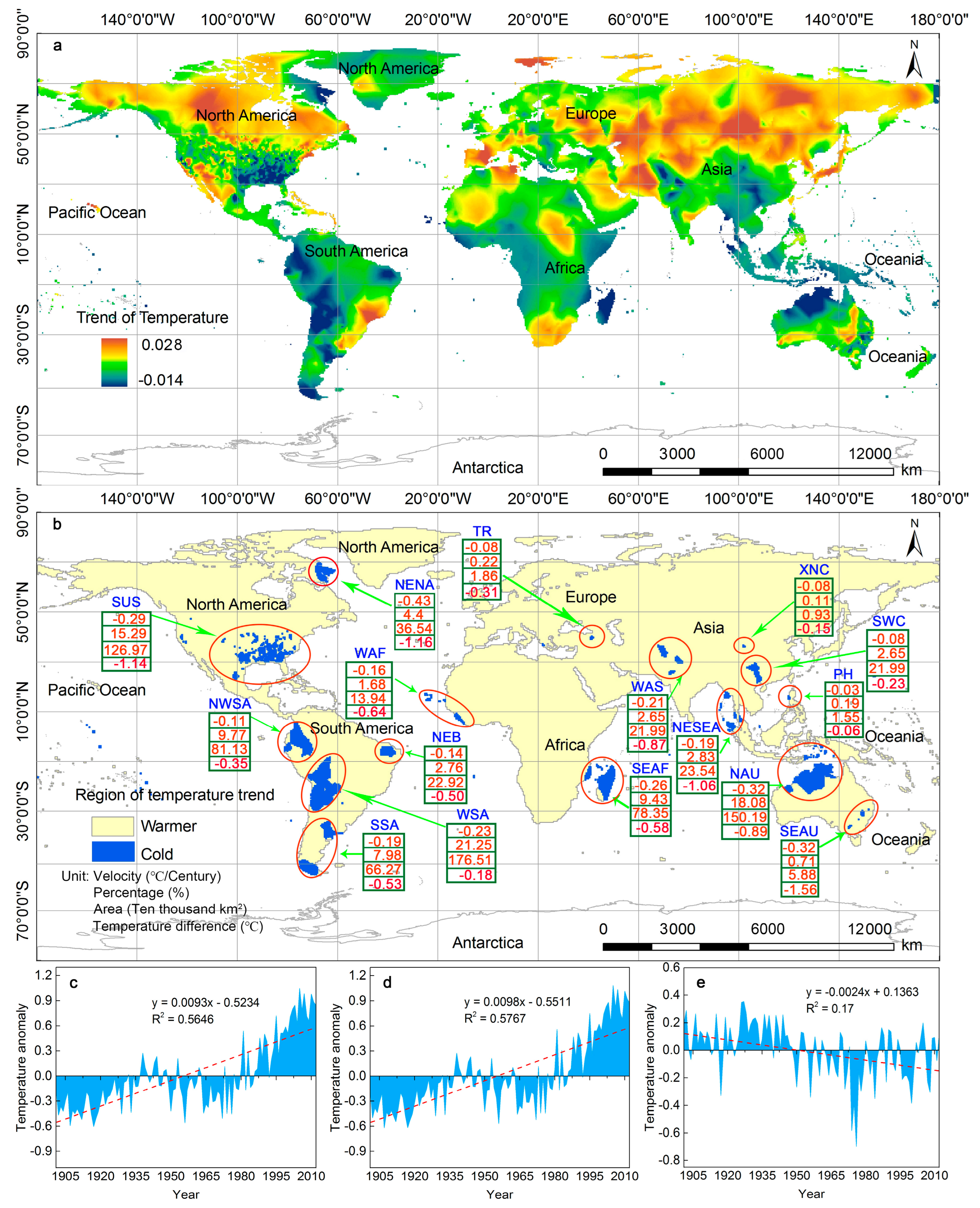
4.1. Change Trends of Global Land Temperature

As shown in Figure 2a, the global land presented a significant warming zone and some concentrated cooling zones. Globally, 126 million km2 of warming land had been detected, accounting for 84.86% of the global land cover, as well as 16 cooling zones (Figure 2b). In China, warming land covered 8,305,500 km2 and accounted for 86% of China’s land area, or 5.57% of the global land cover, respectively. No area had shown a continually stable temperature since the 1900s. The average global land warming rate was 0.93 °C/century, with significant differences in spatial distribution (Figure 2c). The land area showing a warming trend was mainly concentrated in the northern hemisphere and exhibited a meridional distribution feature of more in the east and less in the west.
The temperate continental and Mediterranean climate zones of the northern Eurasian continent and northern North America were the two regions with the most obvious warming trends; they also span the largest area in the world. The warming rate of these regions was 0.98 °C/century (Figure 2d), which was higher than the average warming rate of the global land cover by 5.38%. The temperatures in warming zones showed a fast increase in their rising trends after the 1980s and rose by approximately 0.3 °C within the next 30 years, which were the warmest 30 years of the last 100 years.
The regions showing cooling trends were mainly distributed over the middle and lower latitudes of the coastal areas on both sides of the equator. The average cooling rate of the cooling zones was −0.24 °C/century (Figure 2e), and the maximum cooling rate was −1.40 °C/century, and it was 1.43 times the average rate of global land warming. Although most areas had been warming up rapidly since the 1900s, a slight reduction in temperature had been observed in some areas, indicating that there were many real cooling zones under global warming.

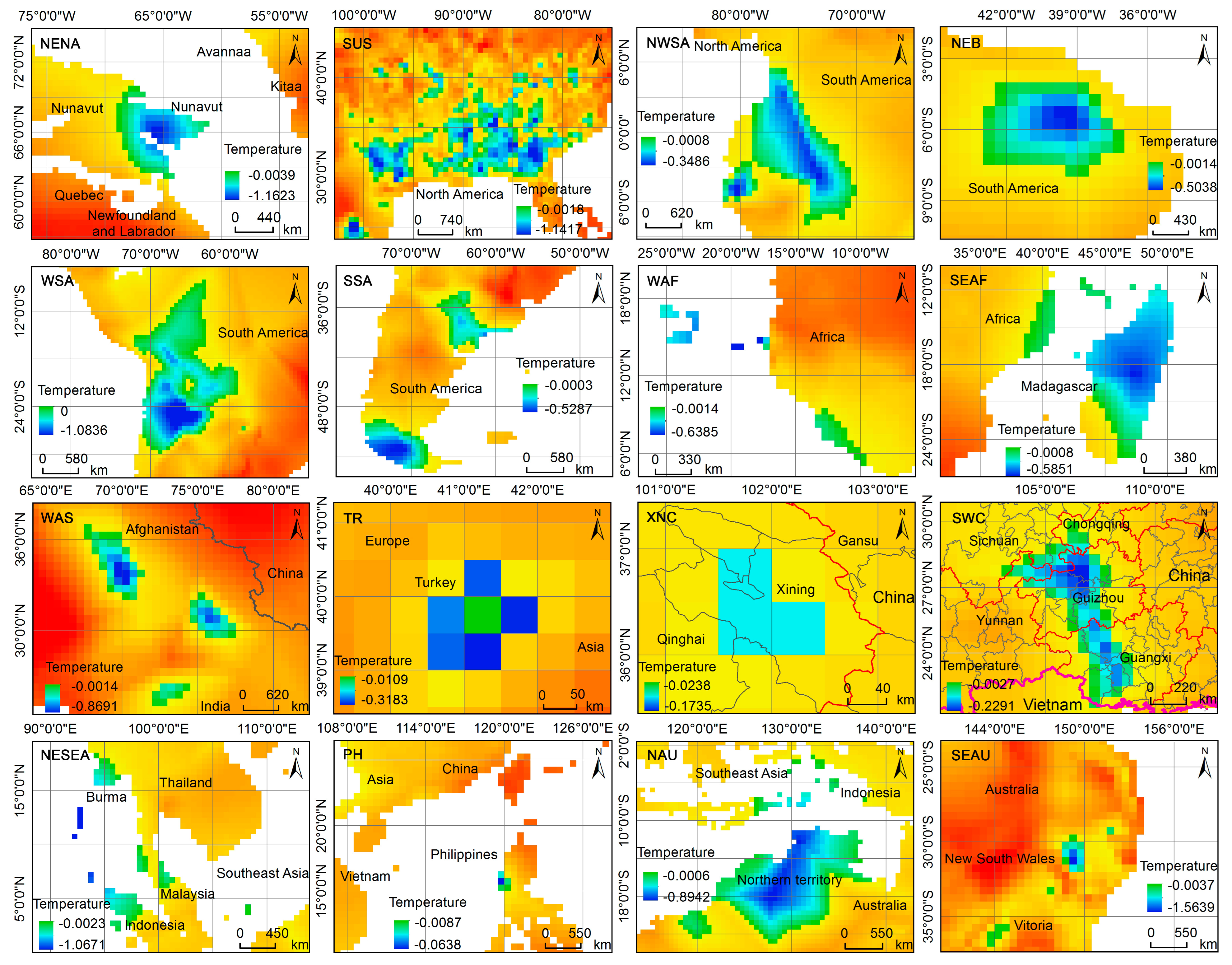
4.2. Spatial Distribution of Cooling Zones

There were significant differences in the spatial distribution of global cooling zones. The cooling zones were found to be intensively distributed across 16 zones, covering five continents and 151 regions of 32 countries (Table 3). In addition, the majority of these zones were distributed in coastal areas, and relatively few were found in inland areas. The cooling zones were most concentrated in South America, with the greatest distribution area covering 3,468,400 km2. This region accounts for 41.76% of the cooling zones. The cooling zones were the most fragmented in Asia, which had a minimum area of only 718,400 km2, accounting for 8.65% of total cooling zones. The largest cooling zone was the WSA (west of South America), and the smallest zone was XNC (Xining, China). These zones span areas of 176,500 km2 and 9300 km2, respectively, and accounted for 21.25% and 0.11% of the cooling zones, respectively.

4.3. Temperature Change Rates of Cooling Zones

There are also significant differences in the cooling rates of cooling zones across different continents (Table 4). The cooling rates of cooling zones in North America and Oceania were relatively large at −0.36 °C/century and −0.32 °C/century, respectively. Regarding the cooling rates (Figure 3), the cooling zones distributed in the Asian continent showed the slowest cooling rate, only −0.11 °C/century. The temperature of cooling zones showed different upward trends before the 1950s, followed by a significant decrease, and they slightly increased after 1979. Since the 1980s, most cooling zones had been warming, with varying periods, durations, and trends.
In addition, each cooling zone shows obvious differences in cooling ranges (Figure 2b), and the cooling range near the sea in each cooling zone is affected by the ocean (Figure 4). The cooling range of SEAU (southeast Australia) was the largest, at 1.56 °C, and the lowest, of PH (the Philippines), was only 0.06 °C. The cooling rate in the center of the inland cooling zone was relatively high. The cooling rate reached its maximum at the center and gradually decreases from the inside out. For cooling zones near the ocean, there was a significant difference in cooling rate between the center and edge of the cooling zone. The closer the cooling zone was to the inland warming zone, the lower the cooling rate. This indicated that each cooling zone was affected by external warming zones, resulting in significant differences in cooling rates between the central and surrounding regions. However, due to the cooling effect provided by the ocean, there was a greater difference in the cooling rate between the center and edge of the cooling zone near the ocean in coastal areas.

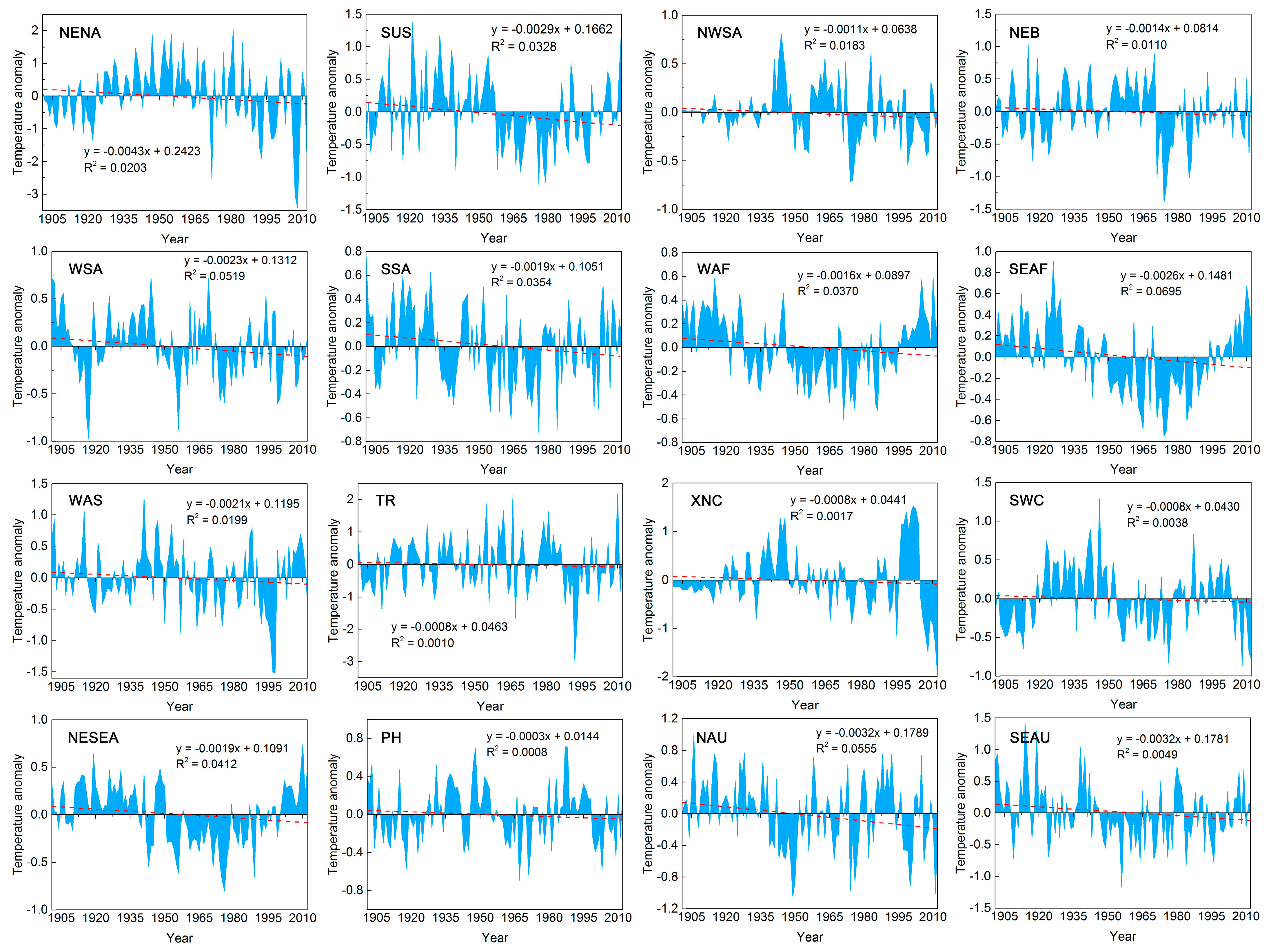
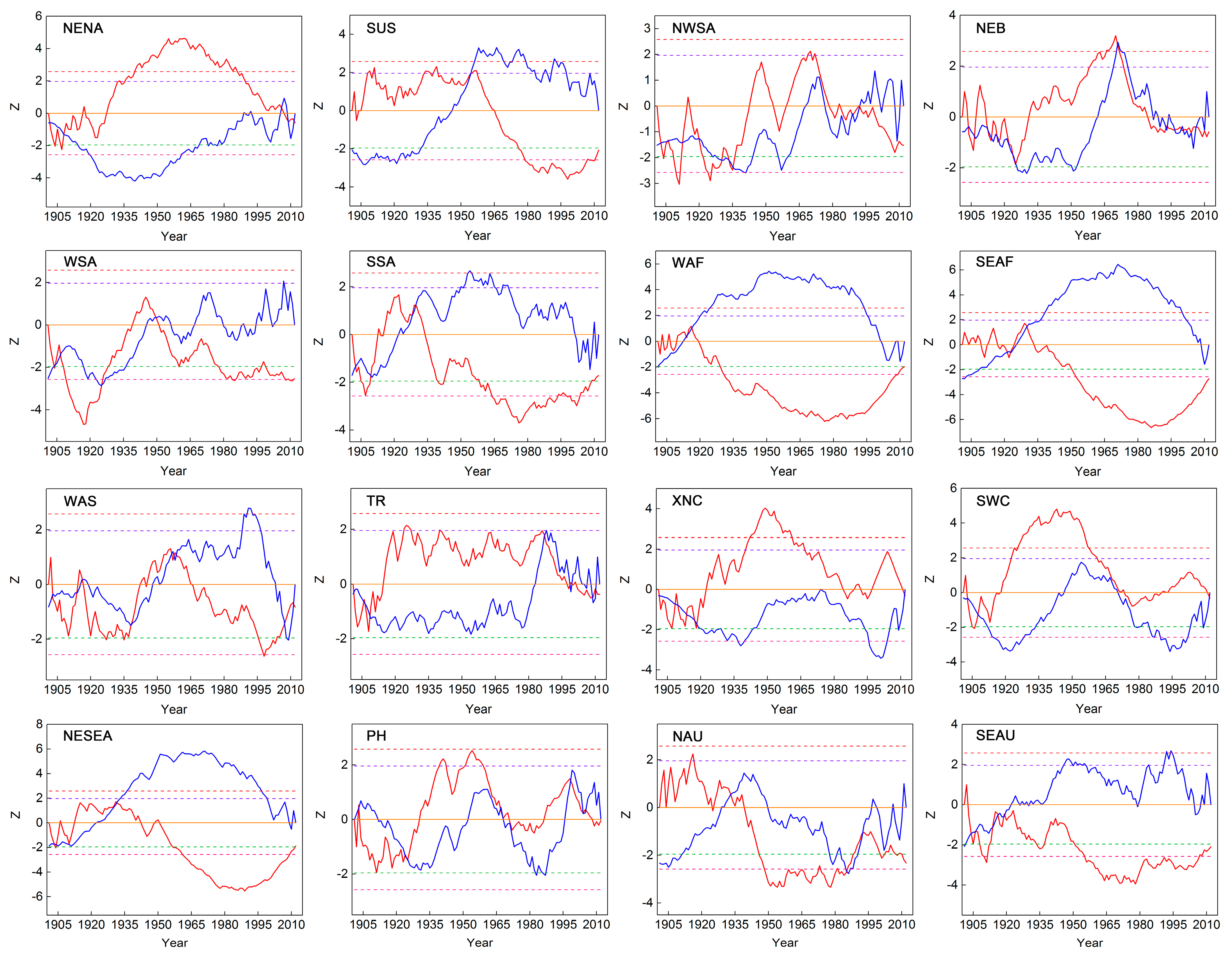
4.4. Evolution of Temperatures in Cooling Zones

4.4.1. Significance

There was a slight difference in the temperature change rates in each cooling zone, and the rates in nearly half of the cooling zones were slow (Table 5). NWSA (northwest of South America) had passed only the 0.1 significance level, and SUS (south United States), SSA (south South America), WAF (West Africa), NESEA (northwest SEA), and SEAU had passed the 0.05 significance level. WSA, SEAF (southeast Africa), and NAU (north Australia) had passed the significance level of 0.01, indicating that the temperature fluctuations in these cooling zones were larger. However, NENA (northeast North America), NEB (northeast Brazil), WAS (West Asia), TR (Turkey), XNC, SWC (southwest China), and PH did not pass the significant trend test, which revealed that the temperature changes of the six cooling zones were characterized by a lack of significant changes and relatively stable cooling trends.

4.4.2. Abrupt Change Point
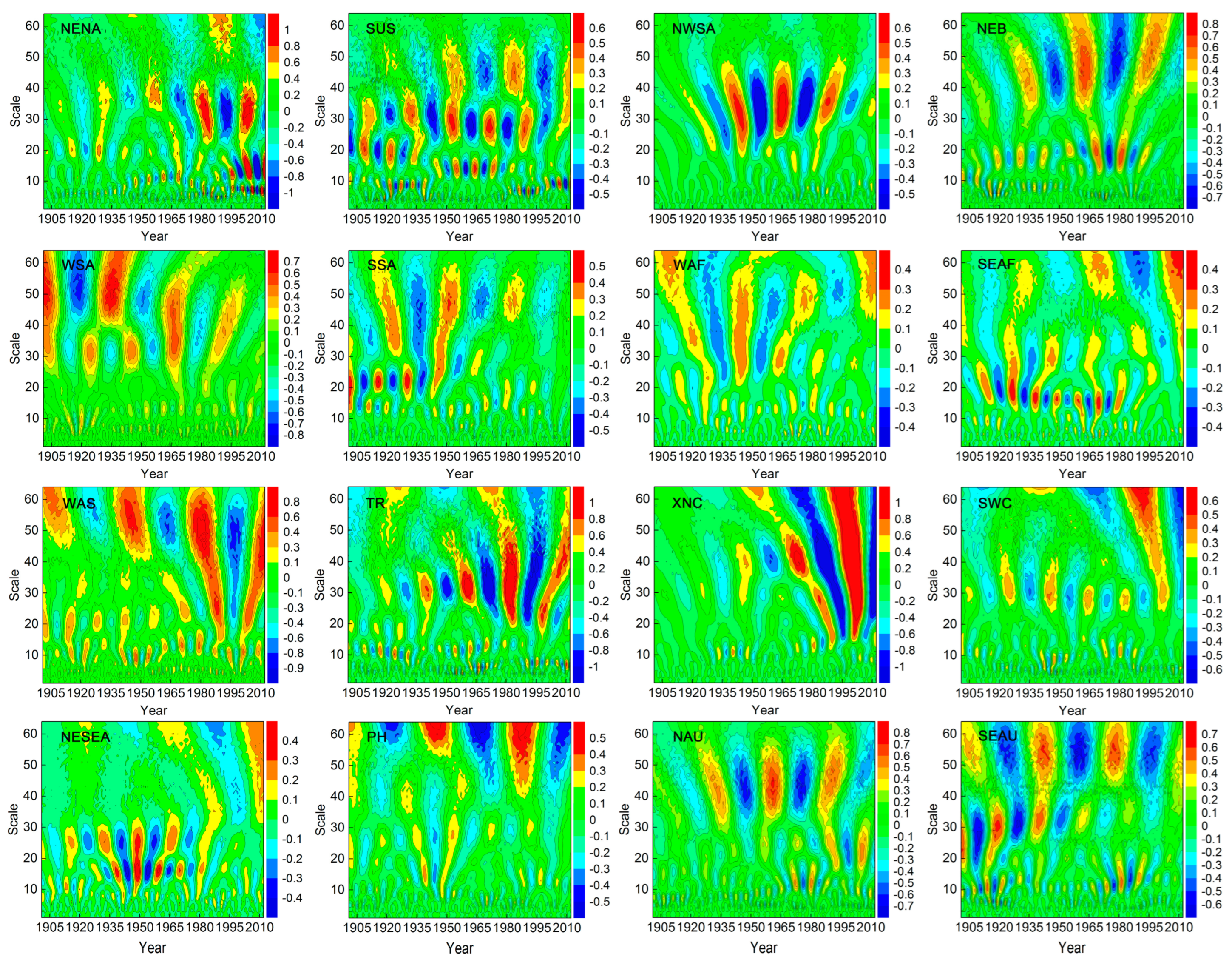
It was found that each cooling zone had multiple mutation points (Table 6), causing several important warming and cooling periods to alternate in time series. The distinct abrupt change points of cooling zones were mainly distributed in the 1930s, 1950s, and 1990s, representing the distributions of two warming periods and one cooling period (Figure 5). Two years of significant warming were 1920 and 1979, whereas 1950 was a cooling year for most cooling zones. Overall, although the temperatures in the cooling zones show a slow downward trend, many cooling zones show a significant increase in temperature over some time periods, indicating that even for cooling zones, temperature changes during specific periods are affected by global warming. However, most cooling zones have continued the trend of cooling. This indicates that although temperature changes in some regions are a response to global warming, the temperature trends in these cooling regions mainly depend on the cooling effects of each cooling region.

4.4.3. Periodicity

The evolution laws of the temperature changes in cooling zones had obvious multi-time scale characteristics (Table 7), which were mainly manifested in periodic changes with different time scales, causing multiple temperature cooling centers during different periods (Figure 6). The main cycle was characterized by small and medium time scales of fewer than 60 years, and the oscillation periods decreased with decreases in the time scale of the main cycle. There were three distinct oscillation periods in the 13 cooling zones, whereas NWSA showed only the first main period, and XNC and PH lacked the third main period, which indicates that the temperatures of each cooling zone have strong and different time scale characteristics. Furthermore, the differences in the land and sea positions had some influences on the multi-time scale characteristics. Specifically, the cooling zones near the sea were greatly influenced by ocean currents and were mainly affected by the small time scale periodicity of fewer than 30 years, whereas the cold zones located relatively far from the sea and less affected by ocean currents were mainly affected by the medium time scales of greater than 30 years.

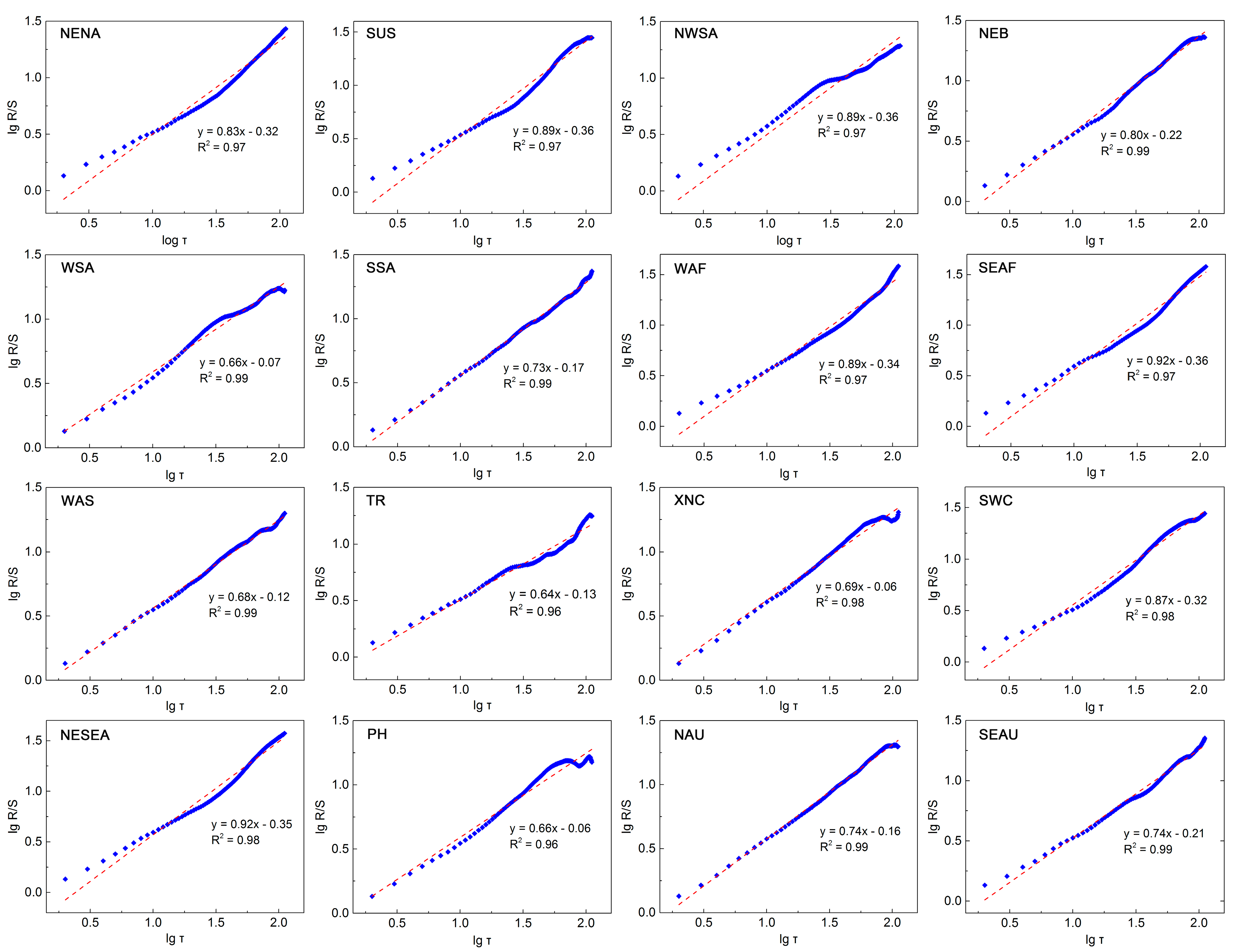
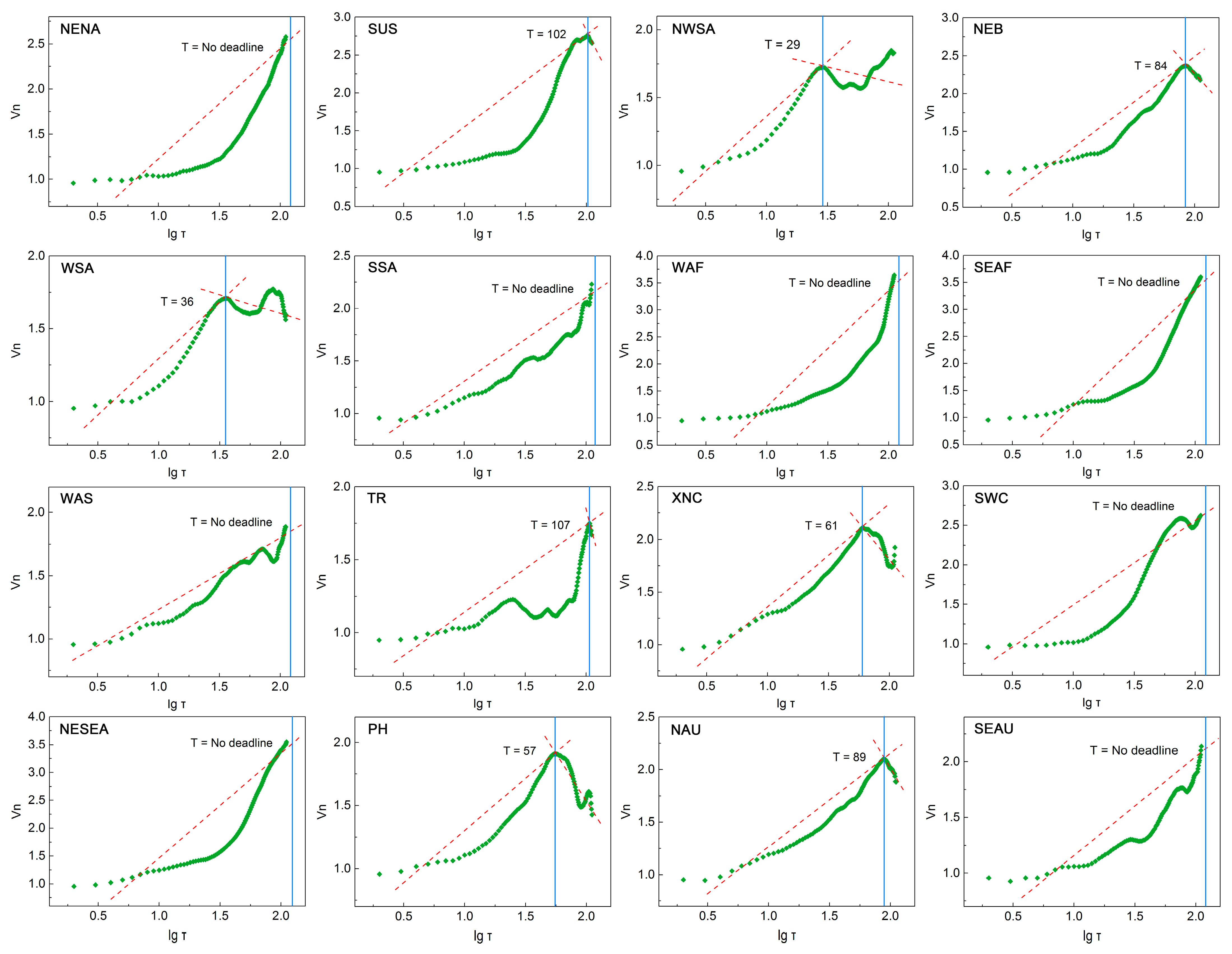
4.4.4. Future Trends

The temperature changes in cooling zones show different positive persistence characteristics (Table 8). The cooling effects of each cooling zone will have considerable differences in the future due to different H values (Figure 7). The degree of persistence of the temperature changes are all above grade II, and the corresponding persistence intensities were all greater than the weakest level. The temperatures in eight cooling zones, namely, NENA, SSA, WAF, SEAF, WAS, SWC, NESEA, and SEAU, covering a total area of 2,684,900 km2 and accounting for 32.33% of cooling zones and 1.80% of the global land area, show continuous cooling. However, the temperatures in the other cooling zones (SUS, NWSA, NEB, WSA, TR, XNC, PH, and NAU), covering a total area of 5,620,600 km2 and accounting for 67.67% of the total cooling zones and 3.77% of the global land area, have a continuous trend with different sustainability and intensity, with time limitations of 102, 29, 84, 87, 107, 61, 36, and 89 years, respectively (Figure 8). These areas will probably continue to cool until 2114, 2041, 2096, 2099, 2119, 2073, 2048, and 2101, respectively, indicating that these cooling zones will be gradually warming in one hundred years or so. Moreover, the cooling trend of the regions with stronger persistence and higher grades of sustainability will become more prominent. A warming trend in the future will become stronger in the regions with shorter sustainability times, weaker sustainability, and lower levels.

5. Discussion

5.1. Comparison with Previous Studies

The average warming rate of the global land area calculated in this study was 0.93 °C/century, and the average warming rate of the terrestrial warming zones was 0.98 °C/century, which were slightly higher than the global warming rate of 0.74 °C (0.56–0.92 °C) that was obtained by the IPCC in their 4th and 5th assessment reports based on the period from 1906 to 2005 [42,43]. Since 1850, the climate had warmed, and the global average temperature had risen by 0.8 °C [44]. Since 1979, the trend of global warming had increased from 0.014 to 0.018 K/yr [45]. Furthermore, the average global surface temperature increased by 0.89 °C from 1880 to 2012, which was especially apparent in the northern hemisphere, where the temperatures in the high latitudes considerably increased. Additionally, the three decades from 1983 to 2012 were the hottest 30 years in the northern hemisphere since 1400 [42,43]. Over the past 100 years, the global average temperature rose by approximately 0.3~0.6 °C [1], and should increase by 1.8–4.0 °C by the end of this century compared to the previous century [2]. In the past 130 years, the trend rate of temperature change in central Asia was 0.073 °C/10a. From the 1960s to the end of 2013, the annual average temperature in China also showed an upward trend, rising by 1.44 °C. Especially after the 1980s, there was a trend of accelerating warming. Except for the Qinghai Tibet Plateau, the warming rate in China increased from south to north [46]. From 1906 to 2005, the annual average temperature in China increased by 0.78 ± 0.27 °C. 2007 had replaced 1998 as the warmest year in nearly a century in China. The temperature on the Qinghai Tibet Plateau in China was on an upward trend in the past century, with a climate warming rate of 0.07 °C/10a [28]. It is worth noting that the observed warming years of 1920 and 1979 in all cooling zones are consistent with those identified by You et al. [47]. From this, it can be seen that the global average land temperature anomaly change rate of 0.93 °C/century and the land warming zone warming rate of 0.98 °C/century are reasonable in this study.
The key contribution of this paper is to detect the existence of 16 cooling zones on a scale of more than 100 years. Although no relevant research has been found before, we can theoretically analyze the scientificity of their existence based on the principles of the surface energy balance of biophysical mechanisms (surface albedo and ET) and surface climate (rainfall, snowfall, and shortwave radiation) [20]. The latitude-specific deforestation experiment shows that afforestation projects in tropical areas will obviously help reduce global warming [22], but it will be counterproductive in high latitudes and temperate regions. This is mainly because the increased carbon sink effect of tropical afforestation and the climate cooling effect of vegetation transpiration exceed the warming effect caused by the reduction of albedo, so local cooling occurs [25]. In high-latitude and temperate regions, afforestation has greatly reduced the surface albedo, and its warming effect on climate has exceeded the cooling effect of vegetation carbon sinks and evaporation due to less precipitation, so warming occurs. The research on the biophysical impact of large-scale deforestation on the surface climate shows that if the global-scale forest is replaced with grassland, a global cooling effect of 1.36 K will be caused by the increase of surface albedo caused by deforestation, while the removal of forests will reduce the evaporation efficiency and surface roughness, which will lead to global surface warmings of 0.24 K and 0.29 K, respectively. This indicates that climate change in various regions of the world is actually a net climate change effect caused by the interaction of many factors. Based on this, we can verify the possibility and scientificity of the detected cooling zones.

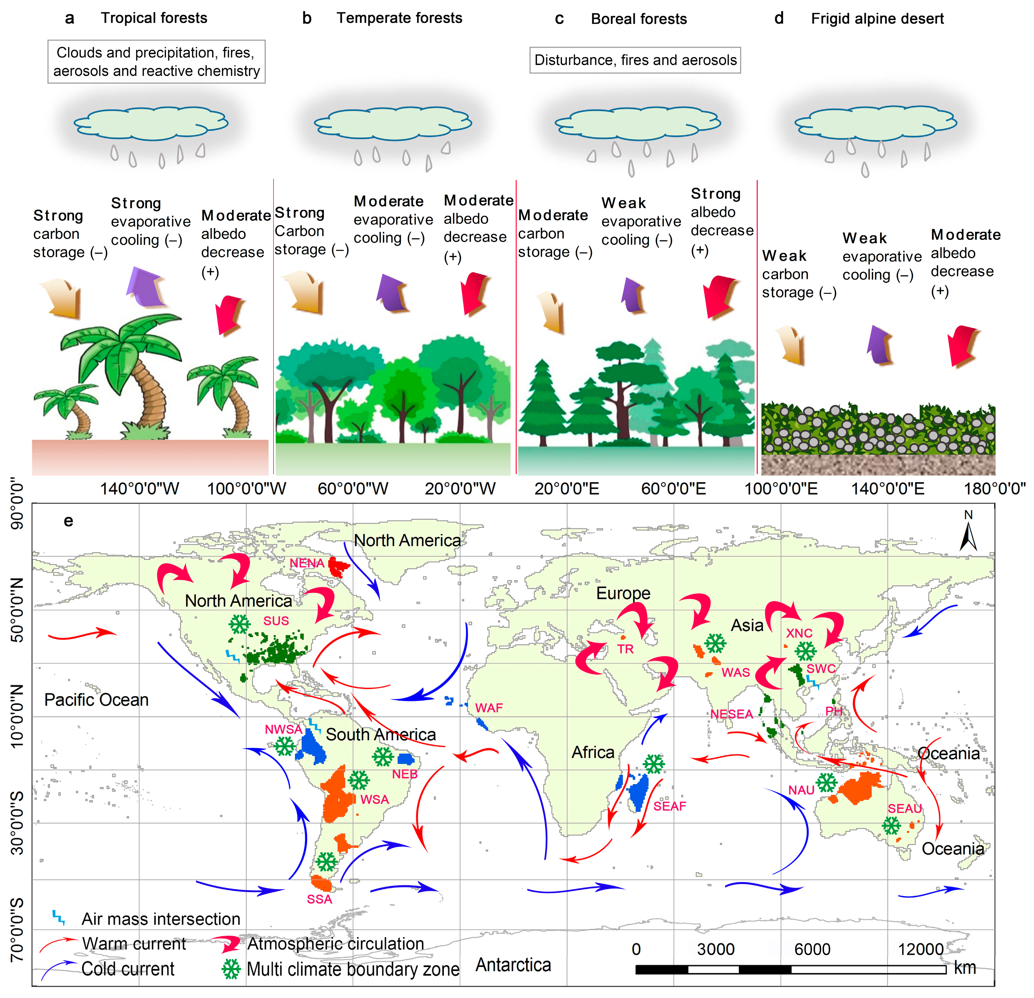
5.2. Impact Factors and Climate Mechanisms

5.2.1. Ocean Currents

The influences of ocean currents are mainly manifested along the coastal areas they flow by (Table 9). Warm currents will weaken the cooling effects in cooling zones or increase the temperatures in warming zones, while cold currents can decelerate the warming in warming zones or maintain or accelerate the continuous cooling in cooling zones. The cooling effects in NENA, SSA, NWSA, and WAF were mainly affected by cold currents, while the warming effects in southern Africa, southeastern South America, southeastern Asia, and southeastern Australia were directly influenced by warm currents. In addition, the influence of the marine hydrological processes directly resulted in the cooling rates of the seaward regions of cooling zones being faster than those in other areas, except those in the central parts of cooling zones.

5.2.2. Atmospheric Circulation

Atmospheric circulation is air mass intersections and the oscillations of atmospheric currents [45], and mainly occurs in the middle and high latitudes of the northern and southern hemispheres and at the boundaries of the multiple climate types (Table 9). Under normal conditions, due to a large temperature difference, the upper air in the Arctic is usually dominated by a low-pressure area system (i.e., the polar vortex), while the relatively warm mid-latitude region is dominated by a high-pressure system. The obvious pressure difference should lead to a strong westerly jet, circling the cold air in the Arctic and preventing its southward expansion, and at the same time, also making the trough ridge activity in the westerlies relatively stable. However, climate change has changed this situation. Due to the amplification effect in the Arctic, compared to other regions, the warming in the Arctic region is more pronounced, resulting in a smaller temperature difference between the polar and mid-latitude regions and a weaker pressure difference. This makes it easier for cold air to invade southward, and the meridional circulation pattern in the mid-latitude regions is strengthened, making it more prone to the occurrence of large ridges and deep troughs, and making it more conducive for polar or high-latitude cold air masses to descend southward along the deep troughs. In this case, the polar cold air mass can even spread directly southward into the middle and high latitudes of Eurasia, causing widespread cooling. In this study, it was detected that the Arctic and its surrounding areas are the regions with the fastest warming trend on global surface land. The pressure difference caused by this will also cause significant cooling when cold air rushes southward. Although these regions still exhibit overall warming characteristics, this cooling effect largely offsets the warming effect. It can be inferred that the TR, WAS, and XNC cooling zones in central Asia are mainly affected by atmospheric circulation. SWC is influenced not only by the frontal rain generated by the intersection of cold and warm air masses, but is also strongly influenced by Arctic oscillation. Arctic oscillation showed a positive phase before the 2000s, limiting the southward expansion of polar cold air and showing a warming trend in SWC. However, the temperature shows a cooling trend due to the increased opportunity for cold air to move south due to the negative phase caused by Arctic oscillation after the 2000s. The temperature at the junction points of multiple climate types fluctuates slightly and tends to decrease slowly due to the influences of the interactions of warm and cold air masses and the atmospheric circulation at the junction of the multiple climatic types, which are obviously distributed in subtropical areas at the boundaries between this climate and temperate zones. We have also obtained the cooling effect of Arctic oscillation based on multiple research reports [48,49], and the results show that Arctic oscillation can significantly affect the long-term trend of land temperature in East Asia, and even the entire northern hemisphere. Although this effect weakens over time, it can offset or partially offset the warming trend of global warming within a time scale of 50 years, and cause cooling phenomena in regions such as northern East Asia [50].

5.2.3. Climate Impact Mechanisms on Land Surface

Warming and cooling actually reflect the positive and negative effects of the net fluxes of surface input and output energies, which are directly manifested as the net climate effect of multiple driving mechanisms [51]. These mechanisms are mainly observed via the comprehensive effects of the heat exchange process between the land and the atmosphere, including the terrestrial climate effects caused by carbon sequestration, evaporation, and surface albedo [20]. And the dynamic comprehensive effect of terrestrial climate effects is the net climate effect at the land surface, and determines the direction of climate change in the absence of greater ocean current or atmospheric circulation, compelling the formation of cooling zones. Therefore, we have proposed four climate mechanisms of net climate forcing on carbon sequestration, evaporation, and surface albedo to reveal the causes of the warming and cooling of the global terrestrial surface, based on previous related studies [17,25,52,53] and several climate mechanisms proposed by Bonan [54] (Figure 9).
In areas with high vegetation coverage and abundant rainfall and heat resources, although the low surface albedo formed by high vegetation can absorb a large amount of solar heat radiation and promote surface temperature rise [55], the strong carbon sink effect and evaporation greatly consume surface heat, which not only offsets the surface temperature increase effect caused by the low surface albedo, but also directly leads to the reduction of surface temperature. The climate service impact mechanism is an intense cooling climate mechanism dominated by strong carbon sequestration and strong evaporation effects, which leads to extremely obvious cooling phenomena in some tropical rainforest areas, such as NWSA, WSA, NEB, SEAF, NEAEA, and PH. Research shows that afforestation and reforestation in tropical, temperate, and cold zones can reduce global warming through carbon sequestration. Although the surface albedo is low in tropical rainforest areas, the surface warming caused by low forest albedo is offset by the cooling caused by strong evaporation [54]. The impact of forests on local temperatures has a clear latitudinal pattern, ranging from strong cooling in tropical regions to moderate cooling in temperate regions, as well as warming in high-latitude regions. However, although these cooling zones are located in areas dominated by strong carbon sinks and strong evaporation effects, they are close to the sea and have a clear distribution of warm currents, which weakens the cooling effect dominated by strong carbon sinks and evaporation. Therefore, the cooling effect has been relatively weak compared to other regions over the past century.
The moderate cooling climate service mechanism dominated by a strong carbon sink effect is mainly manifested in the subtropical and temperate regions, where the vegetation coverage has decreased relative to the tropical rainforest. Here, the surface albedo contributes to the middle warming effect, the evaporation effect has decreased, and the cooling effect is in the middle, which offsets the surface warming effect caused by the surface albedo, but the carbon sink effect is still strong. It is clearly distributed in subtropical regions and their temperate border areas, such as SUS, XNC, SSA, SEAU, and SWC.
In addition, this phenomenon of temperature rise caused by lower surface albedo due to vegetation restoration is very obvious in the Qinghai Tibet Plateau and the global glacier-covered areas. Under the conditions of global warming, the vegetation of the plateau turns green and the cryosphere shrinks, leading to the continuous reduction of the plateau’s surface albedo; that is, the surface darkens as a whole. The darkening of the surface will significantly change the surface energy balance, significantly reduce upward short-wave radiation, increase the surface net radiation, and then enhance the surface sensible heat flux, which will increase the local air temperature [56].
With the increase in latitude, the warming effect of surface albedo is extremely strong in areas with less rainfall and relatively high vegetation coverage, while the two cooling effects of the carbon sink effect and the evaporation effect are reduced, making it difficult to offset the warming effect caused by surface albedo, and leading to the warming effect of cold-zone forests on the global climate. This climate impact service mechanism is a moderate warming climate service mechanism dominated by a low surface albedo effect. It is extremely strong in high-vegetation-coverage areas with less rainfall in temperate zones, especially in temperate continental climate and frigid regions with high vegetation coverage in the mid and high latitudes of the northern hemisphere, northern and southern Africa, and the Mediterranean climate region in the eastern United States, such as NENA, which shows an overall warming phenomenon due to the rapid recovery of vegetation.
In high-latitude areas or desert areas with sparse vegetation coverage, lower vegetation coverage leads to higher surface albedo, thereby increasing surface radiation and weakening the warming effect. Due to the lack of water and light, the carbon sink effect and evaporative cooling effect are extremely weak, which makes it a mild warming climate mechanism dominated by a moderate surface albedo effect. This climate service mechanism is most obvious in the high-latitude cold zone of the northern hemisphere, and the global tropical grassland and tropical desert climate regions, such as WAS.
The climate mechanisms of intense cooling and moderate cooling dominated by strong carbon sequestration and strong evaporation effects are the two main reasons for the formation of inland cooling zones. Although these areas are also affected by the warming effect of lower vegetation albedo in tropical or subtropical areas with abundant rainfall, this positive effect can be offset by higher evapotranspiration, and the net effect is the decline of daytime surface temperature. This cooling mechanism is mainly reflected in the four cooling zones of SWC, SUS, NESEA, and PH. In areas with high vegetation cover at mid to high latitudes, strong ecosystem carbon sinks can result in relatively low atmospheric CO2 concentrations, resulting in a weaker greenhouse effect in the regions. This carbon sequestration cooling mechanism is more evident in the seven cooling regions of WSA, SEAF, SSA, NAU, SEAU, XNC, and WAS. For the cooling areas of SWC, NESEA, and PH, cooling may also be related to the darkening of the surface of the Qinghai Tibet Plateau and its surrounding areas. The darkening of the surface can strengthen the upward movement of the air mass by enhancing the surface sensible heat flux, and then enhance the high pressure in South Asia and the subtropical high pressure in the western Pacific downstream. This not only enhances the summer precipitation in South Asia, but also further exacerbates the current East Asian summer precipitation phenomenon. For SUS, it may also be affected by the darkening of the surface of the Rocky Mountains.

5.3. Limitations and Future Prospects

The reasons for cooling are extremely complex. In addition to the above influencing mechanisms, surface roughness can also affect turbulence between land and air, thereby affecting local diffusion flux. The transition from bare land to vegetation often generates momentum feedback by increasing surface roughness, leading to enhanced turbulent exchange between the surface and the atmosphere, and further leading to a cooling trend on the surface. An increase in surface roughness will also promote convergence and upward movement, as well as an increase in precipitation, thereby promoting transpiration cooling effects. The cooling mechanism of the SWC cooling zone in China may be related to the strong surface and atmospheric turbulence generated by the undulating surface. It is worth noting that the process of vegetation affecting climate is not the result of a single factor, but rather the comprehensive effect of all surface biogeophysical processes. The final climate feedback mechanism formed depends on the balance between different mechanisms, which is also the main reason why the biogeophysical effects of vegetation change on climate are complex and uncertain. For example, in exploring the biogeophysical effects of large-scale deforestation on surface climate, it was found that the net effect of deforestation on climate depends on which physical process dominates. In the cold zone of the northern hemisphere, the albedo effect is stronger, so deforestation will lead to cooling. On the contrary, in the tropics, the sharp temperature rise caused by the decrease of evapotranspiration and surface roughness offsets the temperature drop caused by the increase of albedo, becoming the main influencing factor and warming the region as a whole.
In this study, results show that most zones are jointly affected by many factors with different contributions and formed via different main controlling factors. In addition, the superposition of multiple factors will cause the strengthening or weakening of climate effects and will cause uncertainties regarding the dynamics of the direction and intensity of net climate effects [57], which may lead to significant differences in the cooling rates of different cooling zones and increases or decreases in the number of global cooling zones via their spatial shifts or terminations.
The identified numbers and areas of cooling zones were smaller than the actual values due to the limited resolutions of the available global temperature data. The uneven distribution of meteorological observation stations may affect the research results [58,59]. If the spatial resolution is small enough, more subtle cooling zones are likely to be identified, and their climate mechanisms will be more complex. In the future, there will be not only warming in global terms, but also local cooling due to carbon sequestration, evaporation, surface albedo, and other factors in each place. Furthermore, the trend of local cooling is likely to be strengthened or sustained. Future research should further reveal the interaction mechanisms between the main control factors such as surface albedo, carbon flux, evaporation, and global climate change, and accurately calculate the contribution rates of the main control factors to global climate change, so as to provide a more sufficient theoretical basis for the accurate prediction of future climate change.

6. Conclusions

  • There was amazing cooling; 8,305,500 km2 of land surface has shown a cooling trend since the 1900s, covering five continents and 32 countries, accounting for 86% of the land area in China, and distributed over 16 zones. The average global land surface warming rate was 0.93 °C/century, while the average cooling rate in the cooling zones was −0.24 °C/century. The maximum cooling rate was −1.40 °C/century, and it was 1.43 times the average rate of global land warming (0.98 °C/century).
  • There was a slight difference in temperature change rates in each cooling zone, and the rates in nearly half of the cooling zones were slow. Abrupt change points were detected in all cooling zones, leading to alternating occurrences in time series of several significant heating zones and cooling zones.
  • The cooling zones near the sea were greatly influenced by ocean currents and were mainly affected by a small time scale periodicity of less than 30 years, whereas the cold zones located relatively far from the sea and less affected by ocean currents were mainly affected by the medium time scales of more than 30 years.
  • Eight cooling zones involving 2,684,900 km2 will show continuous cooling in the future, and the rest will probably warm up in 2114, 2041, 2096, 2099, 2119, 2073, 2048, and 2101, respectively.
This study has found 16 cooling zones under global warming conditions, and that 8,305,500 km2 of the global land surface has been cooling since the 1900s. In addition, the spatial locations of 16 huge cooling zones were accurately identified, and cooling trends, abrupt changes, multi-time scale evolutions, and the future sustainability of temperature changes were also revealed. The causes of global cooling phenomena in different cooling zones were further explained based on increased carbon sequestration, evaporation, surface albedo, cooler ocean currents, and cooling caused by atmospheric circulation. This study has provided new theoretical possibilities for the mitigation of global warming and the exploration of surface cooling mechanisms.

Author Contributions

Conceptualization, methodology and validation, L.W. and X.B.; Software and data curation, L.W., Y.T. and Y.L.; Formal analysis, L.W., G.L. and J.W.; Investigation, G.L. and F.C.; Writing, L.W. and F.C. All authors have read and agreed to the published version of the manuscript.

Funding

This research work was supported jointly by the National Natural Science Foundation of China (No. 42261052, No. 42077455, and No. 42167032); Guizhou Provincial Science and Technology Projects (No. ZK(2023)-464 and No. 2022-198); Scientific Research Projects in Higher Education Institutions of the Guizhou Provincial Department of Education (Youth Project) (No. 2022-351); Science and Technology Projects of Tongren City (No. 2022-63); the Strategic Priority Research Program of the Chinese Academy of Sciences (No. XDB40000000 and No. XDA23060100); the Western Light Cross-team Program of the Chinese Academy of Sciences (No. xbzg-zdsys-202101); the Guizhou Provincial Major Science and Technology Achievement Transformation Project (No. 2022-010); the Doctoral Research Startup Fund Project of Tongren University (No. trxyDH2103).

Institutional Review Board Statement

Not applicable.

Informed Consent Statement

Not applicable.

Data Availability Statement

The data analyzed in this study are subject to the following licenses/restrictions: The dataset can only be accessed from the British East Anglia Climatic Research Unit (CRU) (http://crudata.uea.ac.uk/cru/data/hrg/ (accessed on 2 December 2014)) and the China Meteorological Data Sharing Service System (http://cdc.cma.gov.cn/ (accessed on 28 August 2017)). Requests to access these datasets should be directed to [email protected].

Acknowledgments

We would like to thank all the authors and reviewers for their significant guidance and help in writing this manuscript.

Conflicts of Interest

The authors declare no conflict of interest.

References

  1. Ding, Y.H.; Dai, X.S. Temperature variation in China during the last 100 years. Meteorol. Mon. 1994, 20, 19–26. (In Chinese) [Google Scholar]
  2. Peng, S.-S.; Piao, S.; Zeng, Z.; Ciais, P.; Zhou, L.; Li, L.Z.X.; Myneni, R.B.; Yin, Y.; Zeng, H. Afforestation in China cools local land surface temperature. Proc. Natl. Acad. Sci. USA 2014, 111, 2915–2919. [Google Scholar] [CrossRef]
  3. Wang, C.; Wang, Z.; Yang, J. Cooling Effect of Urban Trees on the Built Environment of Contiguous United States. Earth’s Future 2018, 6, 1066–1081. [Google Scholar] [CrossRef] [Green Version]
  4. Zeroual, A.; Assani, A.A.; Meddi, M.; Alkama, R. Assessment of climate change in Algeria from 1951 to 2098 using the Köppen–Geiger climate classification scheme. Clim. Dyn. 2018, 52, 227–243. [Google Scholar] [CrossRef]
  5. Li, C.; Bai, X.; Tan, Q.; Luo, G.; Wu, L.; Chen, F.; Xi, H.; Luo, X.; Ran, C.; Chen, H.; et al. High-resolution mapping of the global silicate weathering carbon sink and its long-term changes. Glob. Chang. Biol. 2022, 28, 4377–4394. [Google Scholar] [CrossRef]
  6. Xiong, L.; Bai, X.Y.; Zhao, C.W.; Li, Y.B.; Tan, Q.; Luo, G.J.; Wu, L.; Chen, F.; Li, C.; Ran, C.; et al. High-resolution datasets for global carbonate and silicate rock weathering carbon sinks and their change trends. Earth’s Future 2022, 10, e2022EF002746. [Google Scholar] [CrossRef]
  7. Xiao, B.Q.; Bai, X.Y.; Zhao, C.W.; Tan, Q.; Li, Y.B.; Luo, G.J.; Wu, L.; Chen, F.; Li, C.; Ran, C.; et al. Responses of carbon and water use efficiencies to climate and land use changes in China’s karst areas. J. Hydrol. 2023, 617, 128968. [Google Scholar] [CrossRef]
  8. Ran, C.; Bai, X.; Tan, Q.; Luo, G.; Cao, Y.; Wu, L.; Chen, F.; Li, C.; Luo, X.; Liu, M.; et al. Threat of soil formation rate to health of karst ecosystem. Sci. Total. Environ. 2023, 887, 163911. [Google Scholar] [CrossRef] [PubMed]
  9. Li, C.; Smith, P.; Bai, X.; Tan, Q.; Luo, G.; Li, Q.; Wang, J.; Wu, L.; Chen, F.; Deng, Y.; et al. Effects of carbonate minerals and exogenous acids on carbon flux from the chemical weathering of granite and basalt. Glob. Planet. Chang. 2023, 221, e104053. [Google Scholar] [CrossRef]
  10. Bai, X.; Zhang, S.; Li, C.; Xiong, L.; Song, F.; Du, C.; Li, M.; Luo, Q.; Xue, Y.; Wang, S. A carbon-neutrality-capacity index for evaluating carbon sink contributions. Environ. Sci. Ecotechnol. 2023, 15, 100237. [Google Scholar] [CrossRef]
  11. Zhang, S.; Bai, X.; Zhao, C.; Tan, Q.; Luo, G.; Wang, J.; Li, Q.; Wu, L.; Chen, F.; Li, C.; et al. Global CO2 Consumption by Silicate Rock Chemical Weathering: Its Past and Future. Earth’s Future 2021, 9, e2020EF001938. [Google Scholar] [CrossRef]
  12. Wu, L.; Wang, S.; Bai, X.; Tian, Y.; Luo, G.; Wang, J.; Li, Q.; Chen, F.; Deng, Y.; Yang, Y.; et al. Climate change weakens the positive effect of human activities on karst vegetation productivity restoration in southern China. Ecol. Indic. 2020, 115, 106392. [Google Scholar] [CrossRef]
  13. Wu, L.; Chen, D.; Yang, D.; Luo, G.; Wang, J.; Chen, F. Response of Runoff Change to Extreme Climate Evolution in a Typical Watershed of Karst Trough Valley, SW China. Atmosphere 2023, 14, 927. [Google Scholar] [CrossRef]
  14. Shen, W.F.; Miou, Q.L.; Wei, T.X.; Kong, C.C. Analysis of temperature variation in recent 130 years in central asia. J. Arid Meteorol. 2013, 31, 32–36. [Google Scholar]
  15. Loarie, S.R.; Lobell, D.B.; Asner, G.P.; Mu, Q.; Field, C.B. Direct impacts on local climate of sugar-cane expansion in Brazil. Nat. Clim. Chang. 2011, 1, 105–109. [Google Scholar] [CrossRef]
  16. Mueller, N.D.; Butler, E.E.; Mckinnon, K.A.; Rhines, A.; Tingley, M.; Holbrook, N.M.; Huybers, P. Cooling of us Midwest summer temperature extremes from cropland intensification. Nat. Clim. Chang. 2016, 6, 317–322. [Google Scholar] [CrossRef] [Green Version]
  17. Jackson, R.B.; Randerson, J.T.; Canadell, J.G.; Anderson, R.G.; Avissar, R.; Baldocchi, D.D.; Bonan, G.B.; Caldeira, K.; Diffenbaugh, N.S.; Field, C.B. Protecting climate with forests. Environ. Res. Lett. 2008, 3, 269. [Google Scholar] [CrossRef]
  18. Lee, X.; Goulden, M.L.; Hollinger, D.Y.; Barr, A.; Black, T.A.; Bohrer, G.; Bracho, R.; Drake, B.; Goldstein, A.; Gu, L.; et al. Observed increase in local cooling effect of deforestation at higher latitudes. Nature 2011, 479, 384–387. [Google Scholar] [CrossRef] [PubMed] [Green Version]
  19. Arora, V.K.; Montenegro, A. Small temperature benefits provided by realistic afforestation efforts. Nat. Geosci. 2011, 4, 514–518. [Google Scholar] [CrossRef]
  20. Kingwell, R.S. Climate change in Australia: Agricultural impacts and adaptation. Australas. Agribus. Rev. 2006, 14, 1–29. [Google Scholar]
  21. Luyssaert, S.; Jammet, M.; Stoy, P.C.; Estel, S.; Pongratz, J.; Ceschia, E.; Churkina, G.; Don, A.; Erb, K.; Ferlicoq, M.; et al. Land management and land-cover change have impacts of similar magnitude on surface temperature. Nat. Clim. Chang. 2014, 4, 389–393. [Google Scholar] [CrossRef] [Green Version]
  22. Bala, G.; Caldeira, K.; Wickett, M.; Phillips, T.J.; Lobell, D.B.; Delire, C.; Mirin, A. Combined climate and carbon-cycle effects of large-scale deforestation. Proc. Natl. Acad. Sci. USA 2007, 104, 6550–6555. [Google Scholar] [CrossRef]
  23. Betts, A.K.; Desjardins, R.L.; Worth, D. Impact of agriculture, forest and cloud feedback on the surface energy budget in BOREAS. Agric. For. Meteorol. 2007, 142, 156–169. [Google Scholar] [CrossRef]
  24. Montenegro, A.; Eby, M.; Mu, Q.; Mulligan, M.; Weaver, A.J.; Wiebe, E.C.; Zhao, M. The net carbon drawdown of small scale afforestation from satellite observations. Glob. Planet. Chang. 2009, 69, 195–204. [Google Scholar] [CrossRef]
  25. Davin, E.L.; Nobletducoudré, N.D. Climatic impact of global-scale deforestation: Radiative versus nonradiative processes. J. Clim. 2009, 23, 97. [Google Scholar] [CrossRef]
  26. Zhang, M.; Lee, X.; Yu, G.; Han, S.; Wang, H.; Yan, J.; Zhang, Y.; Li, Y.; Ohta, T.; Hirano, T.; et al. Response of surface air temperature to small-scale land clearing across latitudes. Environ. Res. Lett. 2014, 9, 034002. [Google Scholar] [CrossRef] [Green Version]
  27. Harris, I.; Osborn, T.J.; Jones, P.; Lister, D. Version 4 of the CRU TS monthly high-resolution gridded multivariate climate dataset. Sci. Data 2020, 7, 109. [Google Scholar] [CrossRef] [PubMed] [Green Version]
  28. Ren, Y.L.; Shi, Y.J.; Wang, J.S.; Zhang, Y.; Wang, S.G. An overview of temperature variation on the Qinghai-Tibetan plateau in the hundred years using UK CRU high resolution grid data. J. Lanzhou Univ. 2012, 48, 63–68. (In Chinese) [Google Scholar]
  29. Wen, X.Y.; Wu, W.S.; Hong, Z.J.; David, V. An Overview of China Climate Change over the 20th Century Using UK UEA/CRU High Resolution Grid Data. Chin. J. Atmos. Sci. 2006, 30, 894–904. [Google Scholar]
  30. Miao, C.; Ni, J.; Borthwick, A.G. Recent changes of water discharge andsediment load in the Yellow River basin, China. Prog. Phys. Geog. 2010, 34, 541–561. [Google Scholar] [CrossRef] [Green Version]
  31. Zuo, D.; Xu, Z.; Yao, W.; Jin, S.; Xiao, P.; Ran, D. Assessing the effects of changes in land use and climate on runoff and sediment yields from a watershed in the Loess Plateau of China. Sci. Total Environ. 2016, 544, 238–250. [Google Scholar] [CrossRef] [PubMed]
  32. Li, Y.; Zhao, M.; Motesharrei, S.; Mu, Q.; Kalnay, E.; Li, S. Local cooling and warming effects of forests based on satellite observations. Nat. Commun. 2015, 6, 6603. [Google Scholar] [CrossRef] [PubMed] [Green Version]
  33. Li, Z.; Xu, X.; Xu, C.; Liu, M.; Wang, K.; Yi, R. Monthly sediment discharge changes and estimates in a typical karst catchment of southwest China. J. Hydrol. 2017, 555, 95–107. [Google Scholar] [CrossRef]
  34. Tian, Y.; Bai, X.; Wang, S.; Qin, L.; Li, Y. Spatial-temporal changes of vegetation cover in Guizhou Province, Southern China. Chin. Geogr. Sci. 2017, 27, 25–38. [Google Scholar] [CrossRef] [Green Version]
  35. Gao, P.; Deng, J.; Chai, X.; Mu, X.; Zhao, G.; Shao, H.; Sun, W. Dynamic sediment discharge in the Hekou–Longmen region of Yellow River and soil and water conservation implications. Sci. Total Environ. 2017, 578, 56–66. [Google Scholar] [CrossRef]
  36. Sen, P.K. Estimates of the regression coefficient based on Kendall’s Tau. J. Am. Stat. Assoc. 1968, 63, 1379–1389. [Google Scholar] [CrossRef]
  37. Pingale, S.M.; Khare, D.; Jat, M.K.; Adamowski, J. Spatial and temporal trends of mean and extreme rainfall and temperature for the 33 urban centers of the arid and semi-arid state of Rajasthan, India. Atmos. Res. 2013, 138, 73–90. [Google Scholar] [CrossRef]
  38. Zhao, Y.; Zou, X.; Gao, J.; Xu, X.; Wang, C.; Tang, D.; Wang, T.; Wu, X. Quantifying the anthropogenic and climatic contributions to changes in water discharge and sediment load into the sea: A case study of the Yangtze River, China. Sci. Total. Environ. 2015, 536, 803–812. [Google Scholar] [CrossRef]
  39. Hao, Y.; Zhang, J.; Wang, J.; Li, R.; Hao, P.; Zhan, H. How does the anthropogenic activity affect the spring discharge? J. Hydrol. 2016, 540, 1053–1065. [Google Scholar] [CrossRef]
  40. Mandelbrot, B.B.; Wallis, J.R. Robustness of the rescaled range R/S in the measurement of noncyclic long run statistical dependence. Water Resour. Res. 1969, 5, 967–988. [Google Scholar] [CrossRef]
  41. Wu, L.H.; Wang, S.J.; Bai, X.Y.; Luo, W.J.; Tian, Y.C.; Zeng, C.; Luo, G.; He, S. Quantitative assessment of the impacts of climate change and human activities on runoff change in a typical karst watershed, SW China. Sci. Total Environ. 2017, s601–s602, 1449–1465. [Google Scholar] [CrossRef]
  42. Solomon, S.; Qin, D.; Manning, M.; Chen, Z.; Marquis, M.; Averyt, K.B.; Tignor, M.; Miller, H.L. Climate change 2007: The physical science basis. Contributions of Working Group 1 to the Fourth Assessment Report of the Intergovernmental Panel on Climate Change. Comput. Geom. 2007, 18, 95–123. [Google Scholar]
  43. Allen, S.K.; Plattner, G.K.; Nauels, A.; Xia, Y.; Stocker, T.F. Climate change 2013: The physical science basis. An overview of the working group 1 contribution to the fifth assessment report of the intergovernmental panel on climate change (IPCC). Comput. Geom. 2013, 18, 95–123. [Google Scholar]
  44. Wheeler, T.; Von, B.J. Climate change impacts on global food security. Science. 2013, 341, 508–513. [Google Scholar] [CrossRef] [PubMed]
  45. Foster, G.; Rahmstorf, S. Global temperature evolution 1979–2010. Environ. Res. Lett. 2011, 6, 526–533. [Google Scholar]
  46. Yue, T.-X.; Zhao, N.; Ramsey, R.D.; Wang, C.-L.; Fan, Z.-M.; Chen, C.-F.; Lu, Y.-M.; Li, B.-L. Climate change trend in China, with improved accuracy. Clim. Chang. 2013, 120, 137–151. [Google Scholar] [CrossRef]
  47. You, W.H.; Duan, X.; Deng, Z.W.; Wu, C.B. The multihierarchical structure and the jumpfeatures of climate changes for the globe, China and Yunnan during the last one hundred years. J. Trop. Meteorol. 1998, 14, 174–180. [Google Scholar]
  48. Serreze, M.C.; Carse, F.; Barry, R.G.; Rogers, J.C. Icelandic Low Cyclone Activity: Climatological Features, Linkages with the NAO, and Relationships with Recent Changes in the Northern Hemisphere Circulation. J. Clim. 1997, 10, 453–464. [Google Scholar] [CrossRef]
  49. Wanng, X.J.; Fang, Z.F. Surface air temperature in China and its relation to Arctic oscillation index. Plateau Meteorol. 2004, 23, 80–88. (In Chinese) [Google Scholar]
  50. Wang, L.; Gong, H.N.; Lan, X.Q. Interdecadal variation of the Arctic Oscillation and its influences on climate. J. Atmos. Sci. 2021, 44, 50–60. (In Chinese) [Google Scholar]
  51. Betts, R.A. Offset of the potential carbon sink from boreal forestation by decreases in surface albedo. Nature 2000, 408, 187–190. [Google Scholar] [CrossRef] [PubMed]
  52. Mildrexler, D.J.; Zhao, M.; Running, S.W. A global comparison between station air temperatures and MODIS land surface temperatures reveals the cooling role of forests. J. Geophys. Res. Atmos. 2015, 116, 337–362. [Google Scholar] [CrossRef]
  53. Lutz, D.A.; Burakowski, E.A.; Murphy, M.B.; Borsuk, M.E.; Niemiec, R.M.; Howarth, R.B. Trade-offs between three forest ecosystem services across the state of New Hampshire, USA: Timber, carbon, and albedo. Ecol. Appl. Publ. Ecol. Soc. Am. 2016, 26, 146. [Google Scholar] [CrossRef] [PubMed] [Green Version]
  54. Bonan, G.B. Forests and climate change: Forcings, feedbacks, and the climate benefits of forests. Science 2008, 320, 1444–1449. [Google Scholar] [CrossRef] [Green Version]
  55. Li, S.; Liang, W.; Fu, B.; Lü, Y.; Fu, S.; Wang, S.; Su, H. Vegetation changes in recent large-scale ecological restoration projects and subsequent impact on water resources in China’s Loess Plateau. Sci. Total. Environ. 2016, 569–570, 1032–1039. [Google Scholar] [CrossRef]
  56. Tang, S.; Vlug, A.; Piao, S.; Li, F.; Wang, T.; Krinner, G.; Li, L.Z.X.; Wang, X.; Wu, G.; Li, Y.; et al. Regional and tele-connected impacts of the Tibetan Plateau surface darkening. Nat. Commun. 2023, 14, 32. [Google Scholar] [CrossRef] [PubMed]
  57. Torres, R.R.; Marengo, J.A. Uncertainty assessments of climate change projections over South America. Theor. Appl. Climatol. 2013, 112, 253–272. [Google Scholar] [CrossRef]
  58. Shen, X.; Liu, B.; Li, G.; Wu, Z.; Jin, Y.; Yu, P.; Zhou, D. Spatiotemporal change of diurnal temperature range and its relationship with sunshine duration and precipitation in China. J. Geophys. Res. Atmos. 2014, 119, 13163–13179. [Google Scholar] [CrossRef]
  59. Wang, H.; Zang, F.; Zhao, C.; Liu, C. A GWR downscaling method to reconstruct high-resolution precipitation dataset based on GSMaP-Gauge data: A case study in the Qilian Mountains, Northwest China. Sci. Total Environ. 2022, 810, 152066. [Google Scholar] [CrossRef]
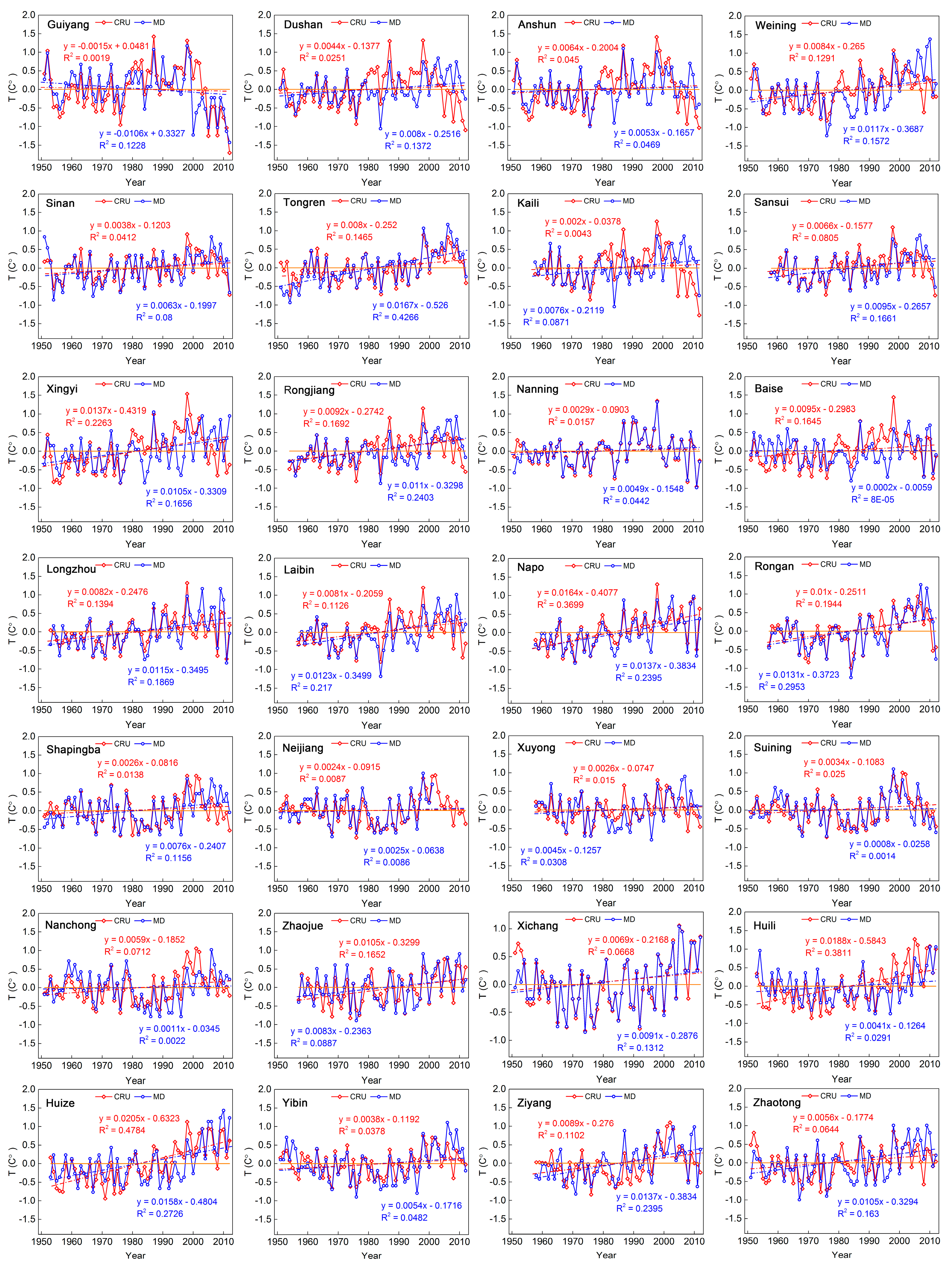
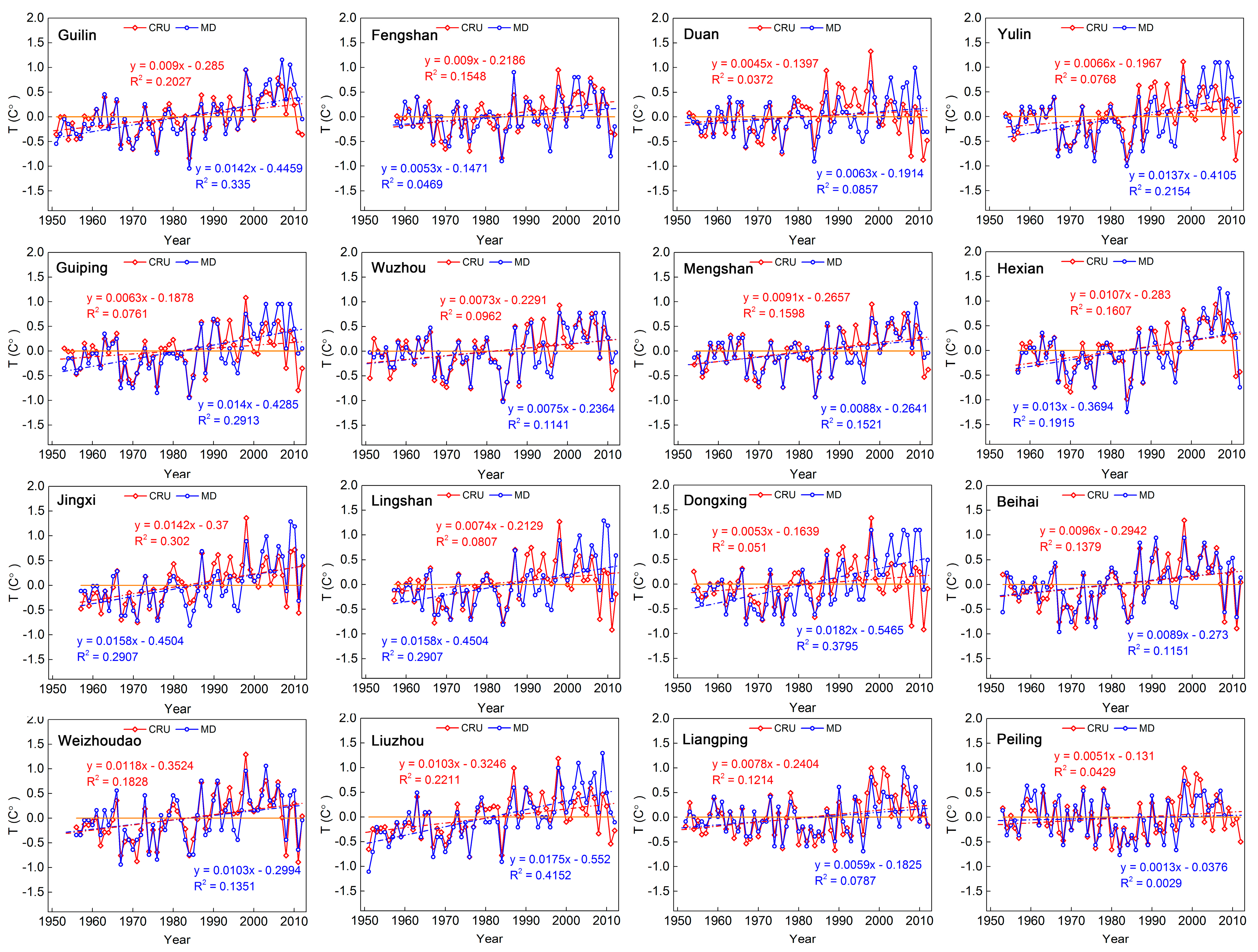
Figure 1. The matching performance between the available measured air temperature data and the corresponding grid mean value of CRU data. The available measured air temperature data are from the 44 meteorological observation stations around SWC (southwest China). The red line is the trend line fitted using CRU temperature data, the blue line is the trend line fitted based on measured temperature data, while the orange line represents the zero mark on the vertical axis.
Atmosphere 14 01156 g001aAtmosphere 14 01156 g001b
Figure 2. Spatial distribution characteristics of change trends of global surface temperature during 1901 to 2012. (a) Spatial distribution of global warming and cooling zones in the world. (b) The temperature change characteristics of global cooling zones with velocity, area and its percentage, and the maximum temperature difference of each cooling zone. The abbreviation of zone codes is shown in Table 3. Temperature change characteristics in global land (c), global warming zones (d), and cold zones (e). The filled blue surface represents the annual temperature anomaly data, while the red surface represents the fitting trend of temperature anomaly changes.
Atmosphere 14 01156 g002
Figure 3. Characteristics of change rates of average temperature in each cooling zone during 1901 to 2012. The filled blue surface represents the annual temperature anomaly data, while the red surface represents the fitting trend of temperature anomaly changes.
Atmosphere 14 01156 g003
Figure 4. Temperature variation amplitude in different cooling zones.
Atmosphere 14 01156 g004
Figure 5. Mann–Kendall test statistics curves of temperature change in cooling zones. The real red line is the UFk curve, the blue solid line is the UBk curve, and the orange red and pink dotted line are the upper and lower limits of the 0.001 significance level, respectively. The purple dotted line is the upper limit of the significance level 0.05, and the green dotted line is the lower limit of the 0.05 significance level. The orange line represents the zero mark on the vertical axis. If the value of UFk is greater than 0, the sequence shows an upward trend, and less than 0 shows a downward trend. When they have exceeded the critical dotted lines, it is shown that the trend of rising or falling is significant, and the range beyond the critical dotted line is the time zone of mutation. If the two curves of UFk and UBk have an intersection and the intersection point is between the critical dotted lines, the time corresponding to the intersection point is the time for the start of the mutation.
Atmosphere 14 01156 g005
Figure 6. The time–frequency distribution of Morlet wavelet transform coefficients real-part contour graphs of the temperature changes in cooling zones.
Atmosphere 14 01156 g006
Figure 7. Fitting curves for the results of Hurst exponent analysis for air temperature in each cooling zone. The coefficient in the formula is the Hurst exponent of H. Blue dots are the logarithmic coordinate points of R/S and t and the red line represents the fitting trend line.
Atmosphere 14 01156 g007
Figure 8. The persistence times (years) for change trends of temperature in each cooling zone. T (year) represents the persistence time of the temperature change trend in the future. If Vn in the Vn – lgt curve is changed with the changing trend of lgt, that is, when the curve shows a significant turning point, the influence of the past state on the future state will disappear and the persistence time of the system T is the corresponding time span τ. green dots are the coordinate points of Vn and lgt. The dashed red line represents the fitting trend line and the vertical blue line is a threshold line added to distinguish future cooling deadline years.
Atmosphere 14 01156 g008
Figure 9. Climate mechanisms of carbon sequestration, evaporation, surface albedo, and influencing factors of ocean currents and atmospheric circulation on global climate change. (ad) represent the climate services in tropical forests, temperate forests, boreal forests, and cold desert regions, respectively. Text boxes indicate key processes with uncertain climate services. The cooling factors of the climate are shown in (e). The four colors displayed in cooling zones represent that the cooling zones were affected by four different climate mechanisms on the surface, respectively. The blue represents intense cooling climate mechanisms dominated by strong carbon sequestration and strong evaporation effects based on the climate services in tropical forests. The green represents the moderate cooling climate mechanisms dominated by strong carbon sequestration effects based on the climate services in temperate forests. The oxblood red represents the climate mechanism of moderate warming dominated by low surface albedo effects based on the climate services in boreal forests. The brownish red represents the climate mechanisms of mild warming dominated by moderate surface albedo effects based on the climate services in cold desert areas. The green snowflake sign indicates that cooling zones near it are located at the junction of various climate types and are affected by air mass intersections.
Atmosphere 14 01156 g009
Table 1. The relevance of the available measured temperature data to the corresponding grid mean value of the CRU data.
StationRVCVMTimeStationRVCVMTime
Guiyang0.75−0.0015−0.01061951–2012Guiping0.820.00630.01401953–2012
Dushan0.520.00440.00801951–2012Wuzhou0.880.00730.00751951–2012
Nanning0.960.00290.00461951–2012Mengshan0.890.00910.00881954–2012
Anshun0.690.00640.00531951–2012Hexian0.890.01070.01301957–2012
Baise0.540.00950.00021951–2012Jingxi0.820.01420.01581957–2012
Yibin0.750.00380.00541951–2012Lingshan0.710.00740.01581957–2012
Zhaotong0.710.00560.01051951–2012Dongxing0.640.00530.01821954–2012
Weining0.670.00840.01171951–2012Beihai0.880.00960.00891953–2012
Longzhou0.840.00820.01151953–2012Weizhoudao0.880.01180.01031956–2012
Ziyang0.650.00890.01371958–2012Liuzhou0.830.01030.01751951–2012
Laibin0.740.00810.01231957–2012Liangping0.810.00780.00591952–2012
Napo0.910.01640.01371958–2012Peiling0.770.00320.00131953–2012
Sinan0.820.00380.00631951–2012Shapingba0.770.00260.00761951–2012
Tongren0.870.00080.01671951–2012Neijiang0.900.00320.00251951–2001
Kaili0.550.00200.00761958–2012Xuyong0.710.00260.00451958–2012
Sansui0.830.00660.00951958–2012Suining0.870.00340.00081951–2012
Xingyi0.510.01370.01051951–2012Nanchong0.700.00590.00111951–2012
Rongjiang0.710.00920.01101954–2012Zhaojue0.830.01050.00831957–2012
Rongan0.840.01000.01311957–2012Xichang0.950.00690.00911951–2012
Guilin0.880.00660.00951951–2012Huili0.760.01880.00411953–2012
Fengshan0.810.00900.00531958–2012Yuling0.750.00660.01371954–2012
Duan0.630.00450.00631953–2012Huize0.790.02050.01581953–2012
Notes: The available measured temperature data are from the 44 meteorological observation stations around SWC (southwest China). VC is the change trend of CRU grid point data corresponding to meteorological stations. VM is the change trend of the available measured temperature data.
Table 2. Classification of Hurst exponent.
GradeHStrength
Positive CorrelationNegative Correlation
I0.50 < H ≤ 0.550.45 < H ≤0.50Weak
II0.55 < H ≤ 0.650.35 < H ≤ 0.45Weaker
III0.65 < H ≤ 0.750.25 < H ≤ 0.35Stronger
IV0.75 < H ≤ 0.850.15 < H ≤ 0.25Strong
V0.85 < H ≤ 10 < H ≤ 0.15Very strong
Table 3. Location characteristics of global cooling zones.
Cooling ZonePositionCountRegion
NENANortheast of North America1Canada (East Nunavut (Iqaluit))
SUSSouth United States24Mexico (southwest Nuevo Leon, south Coahuila, north San Luis Potosí, northeast Zacatecas), America (south and northeast Texas, Louisiana, northwest Colorado, Oklahoma, Arkansas, Mississippi, north Nebraska, west Iowa, northwest Missouri, west and southwest Lino, northeast Indiana, Tennessee, Alabama, Georgia, South Carolina, North Carolina, Kentucky, southwest Pennsylvania, east New Mexico, Ohio)
NWSANorthwest of South America22Colombia (Amazonas, Caquetá, Putumayo, Vaupés, south Guaviare, Nariño, Cauca, Huila, Valle Del Cauca, Tolima, Quindío, Risaralda, Caldas, southwest Meta, west Antioquia, south and central Choco), Peru (Loreto, north Amazonas), Brazil (northwest of Acre, southwest Amazonas), Ecuador
NEBNortheast Brazil4Brazil (Ceará, north Rio Grande do Norte, west Pernambuco, central Piauí)
WSAWest of South America14Argentina (Salta, Catamarca, Jujuy, Tucumán, Santiago—north of Del Estero, northwest of Chaco, northwest Formosa), Chile (Antofagasta, north Copiapó, Iquique), Paraguay (Alto Paraguay), Brazil (Rondônia), Peru (southeast Puno), Bolivia
SSASouth of South America6Argentina (southwest Buenos Aires, east La Pampa, south Córdoba, northeast Río Negro, San Luis, southern Santa Cruz)
WAFWest Africa4Chile (Punta Arenas), Senegal (Dakar), Cape Verde, Sierra Leone,
SEAFSoutheast Africa8Mozambique (Cabo Delgado, Nampula), Madagascar (Toliara (except the southwestern part)), Comoros, Mayotte, Juan De Nova Island, Glorioso Islands, Seychelles
WASWest Asia19Afghanistan (southeast Balkh, southeast Samangan, Baghlan, Parwan, Wardak, Kabul, Logar, Paktia, Khost, Nangarhar, Panjshir, Kapisa, Rugman), India (south Rajasthan, Punjab, Haryana, Delhi, Chandigarh), Pakistan (Central NWFP)
TRTurkey6Turkey (Agri, Erzurum, Kars, Mus, Van, Iğdir)
XNCXining, China1China (east Qinghai (Xining))
SWCSouthwest China21China (southwest Chongqing (Jinjiang, Qijiang, Jiulongpo, Bishan, Nan’an, Dadukou), southeast Sichuan (Ziyang, Luzhou, Yibin), northeast Yunnan (Zhaotong), northwest and south Guizhou (Bijie, Zunyi, Guiyang, Anshun, Qiannan, southwest Guizhou), northwest and southwest Guangxi (Hechi, Nanning, Chongzuo, east Baise, west Laibin))
NESEANorthwest SEA14Indonesia (Aceh, Sumatera Utara, Riau Archipelago), Malaysia (Kota Baba), Thailand (Krabi, Phang Nga, Trang, Phatthalung, Nakhon Si Thammarat), Burma (Bago, Irrawaddy, Yangon)
PHPhilippines2Philippines (Luzon, Lingayen)
NAUNorth Australia3Indonesia (Maluku), Australia (Northern Territory, northeast of Western Australia)
SEAUSoutheast Australia2Australia (central Victoria, northeast New South Wales)
Table 4. Distribution characteristics of cooling zones in continents.
ContinentCooling ZonePercentage (%)Area (Ten Thousand km2)V (°C/Century)
North AmericaNENA SUS19.69163.510.36
South AmericaNWSA NEB WSA SSA41.76346.840.17
AfricaWAF SEAF11.1192.280.21
AsiaWAS TR XNC SWC NESEA PH8.6571.840.11
OceaniaNAU SEAU18.79156.080.32
Table 5. Mann–Kendall test statistics (Z-values) for the velocity of temperature change in cooling zones.
Cooling ZoneZSignificanceChange Trend
NENA−0.61NCooling
SUS−2.06 **YCooling
NWSA−1.53 *YCooling
NEB−0.58NCooling
WSA−2.51 ***YCooling
SSA−1.72 **YCooling
WAF−1.95 **YCooling
SEAF−2.73 ***YCooling
WAS−0.84NCooling
TR−0.36NCooling
XNC−0.32NCooling
SWC−0.30NCooling
NESEA−1.90 **YCooling
PH−0.02NCooling
NAU−2.32 ***YCooling
SEAU−2.08 **YCooling
Notes: The Z index is a standardized M-K statistic to denote the positive (warming) or negative (cooling) trend. * Represents significance at α = 0.1, ** is α = 0.05 and *** is α = 0.01. “Y” represents significant, “N” represents non-significant. The trend significance is distinguished in this study by judging whether the absolute of |Z| is greater than 1.28 with a 90%, 1.64 with a 95% and 2.32 with a 99% significance test.
Table 6. The abrupt change characteristics of temperatures in different cooling zones.
Cooling ZoneMajor Abrupt PointSignificant Abrupt Periods
α = 0.05α = 0.01
IncreasingDecliningIncreasingDeclining
NENA1908 20061939–19891907–19081939–1989
SUS19551910–1912
1934–1936
1937–1939
1955–1958
1976–2011 1978–2011
NWSA1935 19921968–19711910–1912
1922–1931
1933–1936
1909–1912
1923–1926
1934–1936
NEB19711958–1974 1962–1973
WSA1925 1950 1908–1928
1978–1997
1999–2012
1909–1926
1980–1987
1989–1994
2001–2005
2006–2012
SSA1930 1905–1909
1940–1943
1958–2009
1907–1908
1963–2007
WAF1916 1929–2012 1930–2010
SEAF1930 1950–2012 1951–2012
WAS1916 1938 1959 1996–2004 1997–2001
TR19871924–1927
XNC19181940–1967 1941–1962
SWC19081923–19611905–19061924–1959
NESEA1932 1957–2012 1960–2012
PH1925 1968 19991939–1942
1951–1959
1953–1955
NAU1933 1985 19931915–19161946–1989 1947–1987
SEAU1919 1908–1913
1934–1937
1951–2012
1909–1912
1954–2009
Notes: There are 9 cooling zones, NENA, SUS, NWSA, NEB, TR, XNC, SWC, PH, and NAU, that have upward temperature trends that have passed the 0.05 significance levels, and the periods when the upward trends passed the 0.05 significance levels are mainly distributed in the period from 1920 to 1980. There are 5 cooling zones, NENA, NEB, XNC, SWC, and PH, that show increasing temperature trends that passed the 0.05 significance levels, and the significant increases mainly occurred in the period from 1920 to 1990. The cooling zones with downward trends in parts of the years that passed the 0.05 significance level are NENA, SUS, NWSA, WSA, SSA, WAF, SEAF, WAS, SWC, NESEA, NAU, and SEAU, and their significant decreases are mainly concentrated in the 1920s, 1940s, and the period after 1960. The cooling zones that have downward trends that reach the 0.01 significance levels are SUS, NWSA, WSA, WAF, SEAF, SSA, WAS, NESEA, NAU, and SEAU, and their significant declines mainly occurred in the periods before 1940 and after 1980.
Table 7. The multi-time scale characteristics of temperature change in different cooling zones.
Cooling ZoneOscillation Periods (Year)Main Cycles (Year)
PrincipalSecondaryThirdPrincipalSecondaryThird
NENA10–2323–434–913357
SUS20–396–1240–6430945
NWSA20–50 35
NEB33–6411–234–1149198
WSA40–6425–394–16493313
SSA18–3031–6410–18224713
WAF42–5820–406–18513314
SEAF12–2841–6429–40166034
WAS40–6418–387–16532311
TR17–566–99–1732712
XNC35–5420–35 4130
SWC20–359–204–929107
NESEA12–2021–316–1116258
PH21–3216–21 2818
NAU30–6415–306–15452412
SEAU41–6424–409–16543111
Table 8. Results of Hurst exponent analysis and the future sustainability features of velocity of temperature change in each cooling zone.
Cooling ZoneR2HTHistorical ChangeFuture Change
TrendEnd Year of CoolingGradeStrength
NENA0.970.83ColdCoolingIVStrong
SUS0.970.89102ColdCooling2114VVery strong
NWSA0.990.6529ColdCooling2041IIWeaker
NEB0.990.8084ColdCooling2096IVStrong
WSA0.990.6687ColdCooling2099IIIStronger
SSA1.000.73ColdCoolingIIIStronger
WAF0.970.89ColdCoolingVVery strong
SEAF0.970.92ColdCoolingVVery strong
WAS1.000.68ColdCoolingIIIStronger
TR0.960.64107ColdCooling2119IIWeaker
XNC0.980.6961ColdCooling2073IIIStronger
SWC0.980.87ColdCoolingVVery strong
NESEA0.980.92ColdCoolingVVery strong
PH0.960.6636ColdCooling2048IIIStronger
NAU1.000.7489ColdCooling2101IIIStronger
SEAU0.990.74ColdCoolingIIIStronger
Notes: R2 is the goodness of fit with R(t)/S(t) and time lag t, and H is the Hurst indices of them. “–” indicates continuous cooling without time constraints. The persistence degrees of the temperature change include II, III, IV, and V, and the corresponding persistence intensities are weaker, relatively strong, strong, and very strong, respectively. The H values are the highest in SEAF and NESEA, at 0.92, and the lowest in the TR, at 0.64, while the average H of all cooling zone is 0.77, indicating that the overall persistence is strong, but the cooling degree of each cooling zone will make a big difference in the future. SSA, WAF, XNC, and SWC will show extremely strong positive characteristics, with the highest level of V. The persistent features of WAF and SWC are the most prominent, and they will be the two most prominent cooling zones for continued cooling in the future in global terms. The average cycle of the TR cooling zone is the longest, at 107 years, while the NWSA is the shortest, at 29 years. Moreover, SUS has the strongest continuous strength and the highest level of sustainability. At the same time, NWSA has the lowest sustainable intensity, the lowest sustainability level, and the shortest cycle, indicating that NWSA will probably become the earliest cooling zone where the temperature will increase during the next 29 years.
Table 9. Characteristics of coastal directions, climate types, and ocean currents in each cooling zones.
Cooling ZoneSeaward PositionOcean CurrentClimate Type
NENANorth/EastLabrador cold currentTemperate continental
SUSSouth/East Subtropical monsoon, Monsoon humid climate
NWSAWestPeru cold currentTropical savanna, Tropical desert, Alpine, Tropical rainforest
NEBNorthSouth equatorial warm driftTropical savanna, Tropical rainforest
WSAWestPeru cold currentTropical desert, Subtropical monsoon, Monsoon humid, Temperate continental, Tropical monsoon, Tropical rainforest
SSASoutheastFrandk cold current
Peru cold current
Subtropical monsoon, Monsoon humid
WAFWest/SouthwestCanary cold current
Benguela cold current
Tropical rainforest
SEAFAll directionsMozambique warm current, Agulhas warm currentTropical rainforest, Tropical savanna
WASSouthwest Tropical monsoon, Temperate continental, Tropical desert, Alpine
TRNorthwest Temperate continental
XNC Temperate continental
SWCSouth Subtropical monsoon, Monsoon humid
NESEAWestEast Australian warm currentTropical rainforest
PHWestJapan warm currentTropical monsoon
NAUNorthEast Australian warm currentTropical desert, Tropical savanna
SEAUSouth/EastEast Australian warm currentSubtropical monsoon, Monsoon humid
Disclaimer/Publisher’s Note: The statements, opinions and data contained in all publications are solely those of the individual author(s) and contributor(s) and not of MDPI and/or the editor(s). MDPI and/or the editor(s) disclaim responsibility for any injury to people or property resulting from any ideas, methods, instructions or products referred to in the content.

