Article

Precipitation Extremes and Their Links with Regional and Local Temperatures: A Case Study over the Ottawa River Basin, Canada

1
Centre pour l’Étude et la Simulation du Climat à l’Échelle Régionale (ESCER), Université du Québec à Montréal, Montréal, QC H2X 3Y7, Canada
2
Department of Geography, Université du Québec à Montréal, Montréal, QC H2X 3Y7, Canada
3
Department of Earth and Atmospheric Sciences, Université du Québec à Montréal, Montréal, QC H2X 3Y7, Canada
*
Authors to whom correspondence should be addressed.
Atmosphere 2023, 14(7), 1130; https://doi.org/10.3390/atmos14071130
Submission received: 10 May 2023 / Revised: 15 June 2023 / Accepted: 28 June 2023 / Published: 8 July 2023
(This article belongs to the Section Meteorology)

Abstract

:
In the context of global warming, the Clausius–Clapeyron (CC) relationship has been widely used as an indicator of the evolution of the precipitation regime, including daily and sub-daily extremes. This study aims to verify the existence of links between precipitation extremes and 2 m air temperature for the Ottawa River Basin (ORB, Canada) over the period 1981–2010, applying an exponential relationship between the 99th percentile of precipitation and temperature characteristics. Three simulations of the Canadian Regional Climate Model version 5 (CRCM5), at three different resolutions (0.44°, 0.22°, and 0.11°), one simulation using the recent CRCM version 6 (CRCM6) at “convection-permitting” resolution (2.5 km), and two reanalysis products (ERA5 and ERA5-Land) were used to investigate the CC scaling hypothesis that precipitation increases at the same rate as the atmospheric moisture-holding capacity (i.e., 6.8%/°C). In general, daily precipitation follows a lower rate of change than the CC scaling with median values between 2 and 4%/°C for the ORB and with a level of statistical significance of 5%, while hourly precipitation increases faster with temperature, between 4 and 7%/°C. In the latter case, rates of change greater than the CC scaling were even up to 10.2%/°C for the simulation at 0.11°. A hook shape is observed in summer for CRCM5 simulations, near the 20–25 °C temperature threshold, where the 99th percentile of precipitation decreases with temperature, especially at higher resolution with the CRCM6 data. Beyond the threshold of 20 °C, it appears that the atmospheric moisture-holding capacity is not the only determining factor for generating precipitation extremes. Other factors need to be considered, such as the moisture availability at the time of the precipitation event, and the presence of dynamical mechanisms that increase, for example, upward vertical motion. As mentioned in previous studies, the applicability of the CC scaling should not be generalised in the study of precipitation extremes. The time and spatial scales and season are also dependent factors that must be taken into account. In fact, the evolution of precipitation extremes and temperature relationships should be identified and evaluated with very high spatial resolution simulations, knowing that local temperature and regional physiographic features play a major role in the occurrence and intensity of precipitation extremes. As precipitation extremes have important effects on the occurrence of floods with potential deleterious damages, further research needs to explore the sensitivity of projections to resolution with various air temperature and humidity thresholds, especially at the sub-daily scale, as these precipitation types seem to increase faster with temperature than with daily-scale values. This will help to develop decision-making and adaptation strategies based on improved physical knowledge or approaches and not on a single assumption based on CC scaling.

1. Introduction

Accurate knowledge of the fluctuations in extreme events is crucial for effective disaster risk management [1,2,3], specifically in mitigating damages and risks associated with floods. Over the past twenty years, climatic disasters have accounted for 91% of extreme natural events, where 43–44% of the recorded cases were related to floods [4], and 35% were associated with storms that included intense precipitation events (see the overview over the 1970–2018 period in the recent WMO report [5]). Increased episodes of extreme precipitation can lead to an amplification of seasonal river flows in mid- and high-latitude regions [6] or changes in springtime flood characteristics associated with rain-on-snow events during the thawing period (see the study over southern Québec in [7]). This last phenomenon can be particularly noticeable or effective in spring or even in winter, mainly since with global warming, more liquid precipitation (rain-on-snow) will fall in winter and snow will melt more quickly in early spring [8], especially in northern countries such as Canada [9,10]. According to the National Institute of Public Health of Québec [11], floods are the most frequent disasters in Québec, with annual resources that can exceed CAN 15 million.
In this context, the Clausius–Clapeyron (CC) relationship has been used as an indicator of the evolution of extreme precipitation in two separate ways, as highlighted by [12]. Firstly, there is an “observed” scaling that relates the hourly or daily extreme precipitation to the mean daily temperature in the current climate [1,12,13,14,15]. Secondly, there is also a “projected” scaling that establishes the link between changes in extreme precipitation, temperature increase, and climate change [16,17,18,19]. According to the CC theory, saturated vapor pressure of water increases exponentially with temperature. A warmer atmosphere can, in principle, contain more water vapor and, therefore, favor the increased condensation of this vapor, which can result in more intense precipitation [17]. Thus, extreme precipitation is expected to increase at the same rate as the moisture-holding capacity of the atmosphere, with a rate of change of about 7% per degree Celsius, for temperature and pressure values near the surface [8]. Of course, this is just one of the factors involved in the genesis of precipitation, and other complex processes must also be considered at regional and local scales (ex. orographic factors, moist convection, etc.), as well as from the effect of atmospheric circulation that can affect the rainfall–temperature relationship (see [20]).
As revealed in the most recent World Meteorological Organization (WMO) state of the global climate [21] or in the last IPCC sixth-assessment report [22], recent climate changes are generalized with unprecedented levels since two million years ago. The rate of warming trends is increasingly associated with the rise in CO2 and other greenhouse gas concentrations in the atmosphere, leading to an imbalance of energy and, thus, the warming of the atmosphere and ocean [21]. Although extreme precipitation events have increased with rising temperatures over the past two decades [23,24], this intensification is not spatially or seasonally uniform [14,25]. The results obtained from the applicability of the CC relationship with observed and simulated data may vary depending on distinct factors [26]. First, the link between extreme precipitation and air temperature depends on the time scale, as hourly and sub-hourly precipitation increases faster than daily precipitation [1,13,14,15,27]. In addition, the scaling factor may vary depending on the geographic region [14,15,28,29]. Using in situ data, Utsumi et al. [15] determined that daily extreme precipitation increased monotonically with daily temperature (for T > 0 °C) at high latitudes, decreased monotonically in the tropics, and a hook-shaped pattern was observed at mid-latitudes, which is explained as an increase in precipitation at low temperatures followed by a decrease around a threshold of 20 °C.
Other variations in the scaling factor are also observed depending on the season [27,30,31,32] and on the precipitation type, whether convective or large scale [27,30]. In summer, a negative correlation between precipitation and temperature is sometimes observed [33,34], as high-pressure systems usually cause clear skies, low relative humidity values, and a low probability of rain [28]. A prolonged period of dry weather conditions could promote the depletion of soil moisture, a reduction in evapotranspiration from the surface, and therefore, an increase in the temperature of the land surface and the air above it [28,35]. Therefore, the links between extreme temperature and extreme precipitation are seasonally dependent, as recently analyzed over southern Ontario (Canada) by Wazneh et al. [36]. This last study revealed that less precipitation falls in general during cold weather conditions in winter, and more precipitation falls during warm weather in fall.
Even though the knowledge of the links between extreme precipitation and temperature is still incomplete due to the ambiguity of causes and effects [28,37], a more accurate and robust simulation of extreme precipitation can increase our ability to prevent and assess the risk of flooding in the future. A final and crucial element that must be considered when using a climate model to assess the CC relationship is the spatial resolution of the model. Some of the first studies that covered this topic used global climate models (GCMs) [17,19,37,38]. More recently, regional climate models (RCMs) at higher spatial resolution have been incredibly helpful in analyzing the links between extreme precipitation and temperature at regional or even local scales [12,39,40,41,42].
When the model grid is finer than 4 km (very high resolution), RCMs are able to explicitly represent convection without needing a parametrization [26]. These models with explicit convection, also known as “convection-permitting” (CP), have proven to be very useful for improving the quantitative forecasts of extreme precipitation [26], in particular those related to mesoscale convective systems that are better reproduced than in the lower resolution models [43]. Among the most recent studies that have used CP models to better understand the relationship between temperature and extreme precipitation, the following can be mentioned [39,41,44,45,46,47,48].
Large uncertainties remain in the comprehensive understanding of precipitation–temperature scaling, as this is strongly related to the studied region, season, and spatial and temporal processes (i.e., daily vs. hourly or sub-hourly scales; Ref. [49]); hence, more work is needed in that matter. In particular, this is needed at the local or basin scale where floods can occur from precipitation extreme events, using high temporal and spatial resolution of precipitation data from observed stations, reanalysis, or climate simulation products. Hence, the aim of our study is to better understand the applicability of the CC relationship between extreme precipitation and mean daily temperature for the Ottawa River Basin (ORB), located over southeastern Canada, over the current climate. This basin scale is regularly affected by spring floods, as in 2017 and 2019 (see [7]), or flash flood events within small-scale watersheds associated with intense thunderstorms (as in 26 June 2021 with more than 55 mm of rainfall over less than 2 h near Mont-Tremblant in Quebec; Ref. [50]).
Assessing the response of precipitation extremes to temperature increases is particularly important and quite challenging in northern regions where the observed temperature trends significantly exceed the global trend [51], along with the fact that temperature ranges are quite extensive and with different types of precipitation implying various physical processes. In fact, uncertainty in scaling precipitation extremes and temperature using the CC relationship may arise from the choice of data and methods or it can be due to more complex thermodynamic and dynamic factors [52]. The relations among water vapor, precipitation, and temperature are quite often used to characterize to both common/regular and extreme weather events [53]. Nevertheless, an accurate simulation of these meteorological variables is very challenging because of the possible interdependence and feedback among them [36].
Here, we use four simulations at different spatial resolutions of the last two versions of the Canadian Regional Climate Model (CRCM, versions 5 and 6), developed at the ESCER (Étude et Simulation du Climat à l’Échelle Régionale) center of the Université du Québec à Montréal (UQAM). This will also be combined or compared with two recent versions of high-resolution reanalysis products, ERA5 [54] and ERA5-Land [55], from the European Centre for Medium-Range Weather Forecasts (ECMWF). In this study, the “observed” scaling will be analyzed based on the assumption that relative humidity remains constant with increasing temperature, and that the most intense precipitations are primarily determined by specific humidity [29,38]. The methods used to address the research question are based on Lenderink et al. [12,27] for precipitation extremes and temperature pairs analysis, and on Hardwick Jones et al. [13] for exponential relationships to link the evolution of the 99th percentile of hourly and daily precipitation and the temperature change. We will study the variations in this relationship according to the spatial resolution of the model, the temporal scale, and the season of the year; we will also investigate the physical causes that could explain the hook-shaped behavior (if any) obtained for the summer season. The paper is organized as follows. In Section 2, we detail the data and methods along with the study region, the various data products, and the methodology used to obtain the results analyzed in Section 3. Finally, the discussion and the conclusions are presented in Section 4. The main contributions of the study confirm recent work suggesting that very high spatial resolution simulations are needed to evaluate and identify temperature/precipitation relationships, and caution is needed regarding the applicability or generalization of the CC scaling in the study of precipitation extremes.
The findings also suggest that as global temperatures continue to rise, hourly precipitation extremes may increase at rates exceeding the CC scaling, potentially leading to more frequent and intense precipitation events.

2. Data and Methods

2.1. Study Region

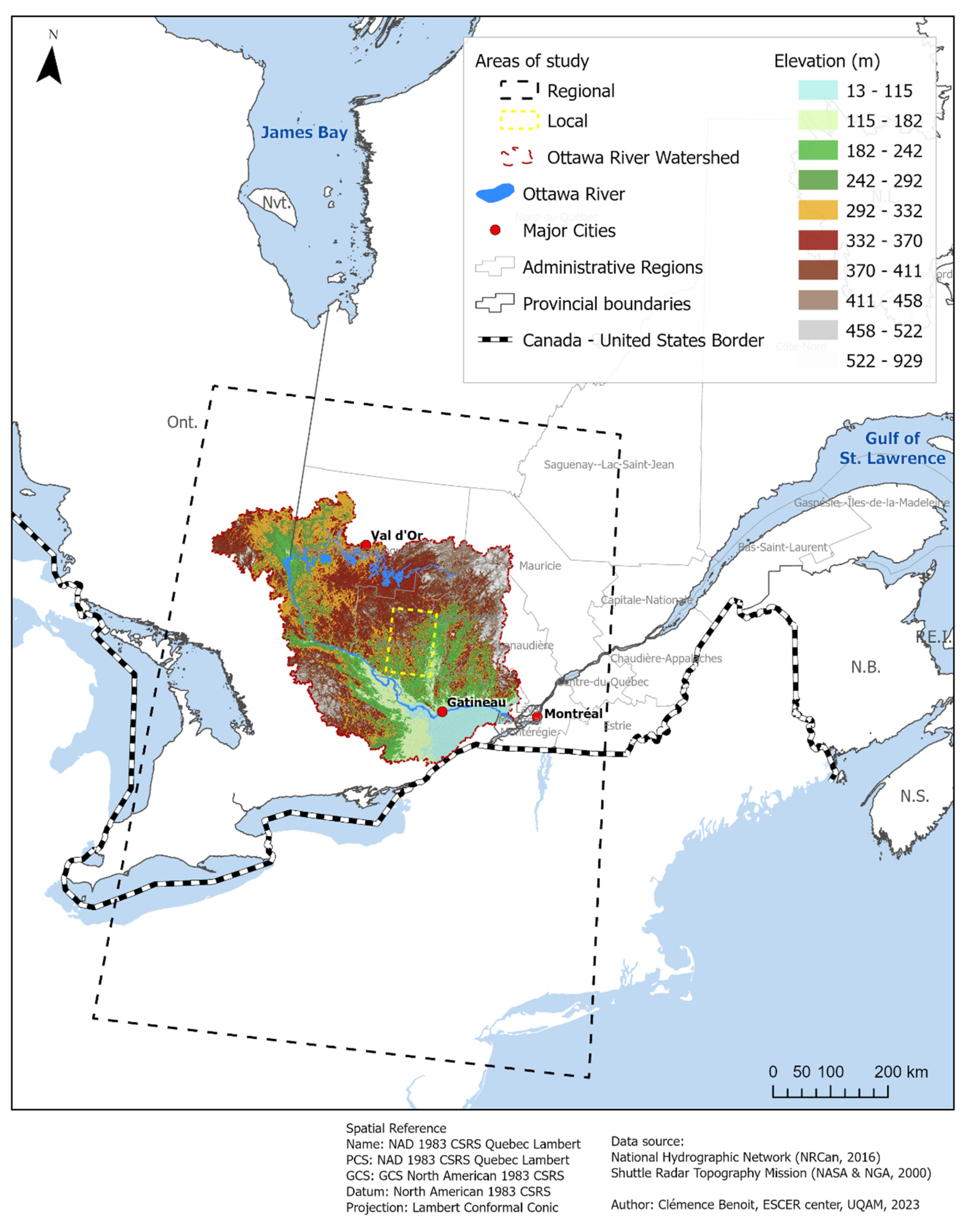
The study region, shown in Figure 1, covers three different areas in which various analyses will be conducted, namely, using these domains:
  • Domain #1 covers a large area located between 40 and 50 °N in latitude and between 82 and 72 °W in longitude. It encompasses the southern part of the provinces of Québec and Ontario, and the northeastern part of the United States. It was chosen to compare the spatial distribution of the scaling factor (α) in the sub-domain #2 with the surrounding areas.
  • Domain #2 corresponds to the Ottawa River Basin (ORB) itself. Located in southeastern Canada, the ORB occupies an area of 146,334 km2, of which 65% is in Québec and 35% in Ontario [56]. The forest represents 77% of the total surface coverage, 19% corresponds to the hydrographic network (rivers, lakes, and wetlands), while agricultural and urban areas occupy 3% and 1% of the territory [57]. Domain #2 corresponds to the main area of our study used for the analysis of precipitation–temperature scaling.
  • Domain #3 corresponds to a small area within the ORB area, extending between 46 and 47 °N and 77 and 76 °W. It was chosen for the analysis of the links between extreme precipitation and the atmospheric circulation in summer.
Figure 1. Three regions used in this study (domain #1 in black dash, domain #2 (ORB), and domain #3 in yellow) [58,59].
Atmosphere 14 01130 g001

2.2. Data

Two different versions of the Canadian Regional Climate Model (CRCM), versions 5 and 6 (i.e., CRCM5 and CRCM6), are used in the present study. The CRCM5 has been widely used for simulations in the context of climate change [60,61,62], in particular under the Coordinated Regional Climate Downscaling Experiment (CORDEX; Refs. [63,64]). This fifth generation of the CRCM is based on a limited-area model (LAM) of the third version of the Canadian Global Environment Multiscale (GEM) model used for the Numerical Weather Prediction (NWP) at Environment and Climate Change Canada (ECCC, Refs. [65,66]). The CRCM5 includes the Canadian Land Surface Scheme CLASS 3.5 [67] and the thermodynamic model Flake, which simulates the temperature of lakes. A detailed description of the CRCM5 is available in [68,69,70]. In this study, we use precipitation and temperature fields of three simulations that were performed with the CRCM5 for the North America region at different resolutions (0.44°, 0.22°, and 0.11°) within the framework of the North America–CORDEX [63,71]. These three simulations are driven at 3 h intervals by the ERA-Interim reanalysis [72] for both atmospheric and oceanic boundary conditions. These cover the 1979–2014 period (see details in Table 1).
The recent CRCM6 version is based on the fifth version of the GEM (Global Environmental Multiscale) model [65,66,73,74] developed by the “Recherche en prévision numérique (RPN)” at ECCC, and currently used for numerical weather prediction (NWP) in Canada. This simulation includes the most recent version of the land-surface scheme CLASS 3.6 model [67,75,76,77] with soil layers down to 10 m, the microphysics P3 (Predicted Particle Properties; Refs. [78,79]) and the subgrid cloud fraction and precipitation module [80]. The CRCM6 simulation uses a horizontal grid mesh of 0.0225° (around 2.5 km) and a “convection-permitting” configuration with no deep convection scheme, i.e., only shallow convection is used (as in [74]). This covers the 2014–2022 period, but only the complete 7-year time window (2015–2021) is used in the present study. This is driven (every 1 h) by the recent ERA5 reanalysis [54], for both atmospheric and oceanic boundary conditions. This higher resolution will be used to evaluate the added values of the convection-permitting simulation or similarity/dissemblance in CC relationships with respect to coarse-scale simulations.
The two variables used from the simulations of the CRCM5 and CRCM6 were 2 m-air temperature and total precipitation. Total precipitation corresponds to accumulated (liquid and solid) values from large-scale and convective precipitation amount, at both hourly and daily timescales.
The ERA5 and ERA5-Land reanalysis products from ECMWF are also used to allow the intercomparison with the simulations from different resolutions and the two CRCM versions. These two products were extracted from the Copernicus Climate Change Service Climate Data Store site [81]. The ERA5 reanalysis [54] is the fifth generation of the atmospheric reanalysis on a global scale at around 31 km of horizontal resolution of the ECMWF, while ERA5-Land [55] provides the evolution of the land component of ERA5 at an improved resolution of approximately 9 km. The description of each variable (temperature and precipitation) used from the two reanalysis products is also presented in Table 1.
Two other meteorological fields of ERA5, the geopotential height at 500 hPa and the mean sea-level pressure (see Table 1), were used to analyze the possible links between extreme precipitation and large-scale atmospheric circulation, and its influence on the precipitation–temperature scaling behavior.

2.3. Precipitation–Temperature Scaling Approach

We used the methodology proposed by Lenderink et al. [13], known as the “Binning Method”, which has been applied in numerous studies [12,14,15,29,40]. This method consists of creating temperature and precipitation pairs on wet days, grouping the data pairs in temperature bins, and then calculating the most extreme (i.e., 99th) percentiles of precipitation for each temperature interval.
In our study, the daily mean temperature was chosen instead of the temperature during the precipitation event. According to Lenderink et al. [13], this provides a good approximation of the temperature of the air mass, without considering the variations that it could take place due to the precipitation event itself. Regarding the precipitation data, the maximum hourly precipitation intensity over a 24 h period was chosen to analyze the behavior of hourly extreme precipitation, and the cumulative precipitation intensity over a 24 h period was used to analyze the daily extreme precipitation. To avoid the inclusion of “trace” precipitation values, a threshold of 0.3 mm was used to define wet days. This procedure is widely used in Canada to eliminate exceedingly small precipitation amounts [82].
The approach chosen to create the bins is the one proposed by Lenderink et al. [28] that involves the creation of overlapping temperature bins of 2 °C width, every interval of 1 °C. The temperature average is chosen as the representative value of the bin, and then the 99th percentile of precipitation (hourly and daily) is calculated for each bin created.
To study the applicability of the CC equation, Hardwick Jones et al. [14] proposed an exponential relationship (see Equation (1)) to link the evolution of extreme precipitation (99th percentile) and the temperature change ΔT, where α represents the rate of change of precipitation as a function of the temperature change; α = 0.068 is equivalent to the 6.8%/°C scaling from the CC relationship. To find the α value, an exponential regression is applied to the temperature and precipitation data (99th percentile), fitting a linear least squares regression to the logarithm of the percentile of precipitation log (P2) as a function of ΔT. Thus, log 1 + α corresponds to the slope of the function and log (P1) corresponds to the point of intersection of the regression line with the ordinate axis. The same methodology was applied on a seasonal scale to analyze the possible variations in the behavior of the CC relationship during the year.
P 2 = P 1 1 + α Δ T log P 2 = log P 1 + Δ T x log 1 + α
In this study, the scaling factor was calculated for all grid points using the least squares method, but only the point where the correlation coefficient between the two variables was statistically significant at the 5% level (i.e., p-value ≤ 0.05) was selected. After calculating the parameters: slope and intercept of the regression line, the Pearson correlation coefficient (coef_r), the p-value for a hypothesis test whose null hypothesis is that the slope is zero, using Wald Test with t-distribution of the test statistic, and the standard error (std_err) of the estimated slope (gradient), under the assumption of residual normality, only points where p-value was greater than 0.05 were converted to NaN (Not a Number).

2.4. Analysis of the Links between Precipitation Extremes and Atmospheric Circulation in Summer

In this analysis, only the simulation with the highest spatial resolution of the CRCM5 (0.11°) is used. Here, the research is oriented towards the analysis of the particular precipitation–temperature scaling, observed in the summer season.
Before performing this analysis, the ERA5 data 500-hPa geopotential height (GZ-500) and mean sea-level pressure (MSLP) were interpolated onto the same grid as the data from the CRCM5 output at 0.11° using a bilinear interpolation. For the summer months, the GZ-500 and the MSLP are described from climatological charts (1981–2010) and anomalies. These anomalies were calculated for days for which domain #3 (shown in Figure 1) had temperatures in the following intervals: (A) T < 15 °C, (B) 15 °C ≤ T < 25 °C, and (C) T ≥ 25 °C.

3. Results

3.1. Annual Behavior of the Scaling Factor (α) between Extreme Precipitation and Daily Temperature

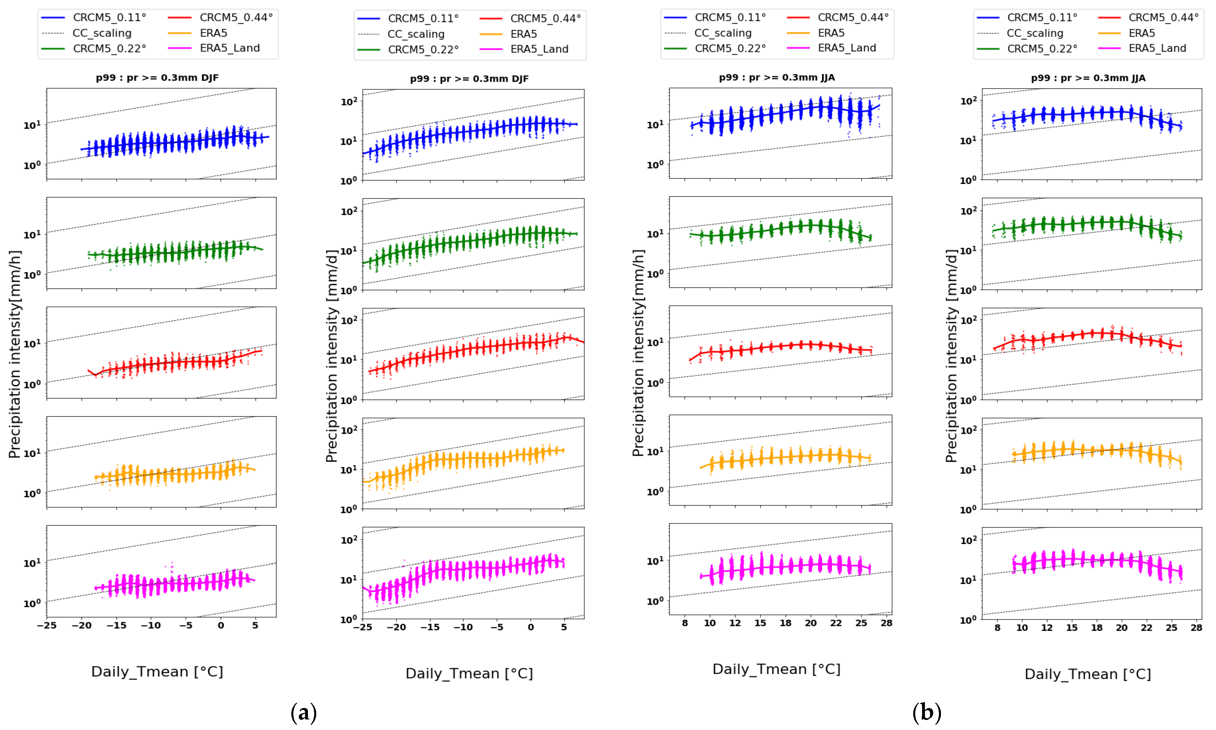
Figure 2 shows the evolution of the 99th percentile of hourly (a) and daily (b) precipitation as a function of the daily mean temperature. Here, all of the grid points of the CRCM5 and reanalysis were grouped by temperature intervals of 2 °C, every 1 °C, and represented as a cloud of points, where the solid line corresponds to the mean value. Note that daily mean temperature (Tmean) is used in the following and corresponds to average values from all 3 or 1 h fields (see Table 1). In general, the precipitation increases up to 20 °C, where there is an inflection point followed by a decrease or stabilization of the 99th percentile of precipitation. This hook-shaped behavior described in Section 1 is especially remarkable for hourly precipitation (Figure 2a) in the higher resolution simulation (CRCM5_0.11°), much less pronounced for the simulation at lower resolution (CRCM5_0.44°), and almost absent in the reanalysis. Concerning the evolution of daily extreme precipitation (Figure 2b), the model output also shows the hook-shaped behavior. However, this behavior is less pronounced than in the case of hourly extreme precipitation. At this step, we could say that the moisture-holding capacity, described in the CC relationship, does not seem to be the only factor to consider when explaining the evolution of extreme precipitation for temperatures exceeding 20 °C in the study region.
The box plots shown in Figure 3 represent the scaling factor α (%/°C) for each grid point within the ORB (domain #2). The parameter α was calculated from the linearization of the exponential function presented in Equation (1) (Section 2), between the hourly and daily extreme precipitation and Tmean. The scaling factor is close to the value of 6.8%/°C for hourly extreme precipitation simulated by the CRCM5_0.11°, with a clear tendency to decrease for both model runs at coarse-scale resolutions and the reanalyses. It can also be noted that for several grid points at 0.11°, the scaling factor is sometimes greater than the value of 6.8%/°C, a super-CC behavior. Unlike hourly precipitation, the scaling factor α for daily extreme precipitation is systematically and consistently sub-CC (lower than 6.8%/°C) in all box plots, whatever the resolution of the CRCM models and reanalysis products, with more similar features among them than for hourly precipitation. Again, there is a decrease in the α parameter for the CRCM5 simulations with coarse resolutions and for the reanalyses. In addition, the number of extreme values of the scaling factor has decreased compared to hourly precipitation in all cases, and the differences between all products are also smaller.
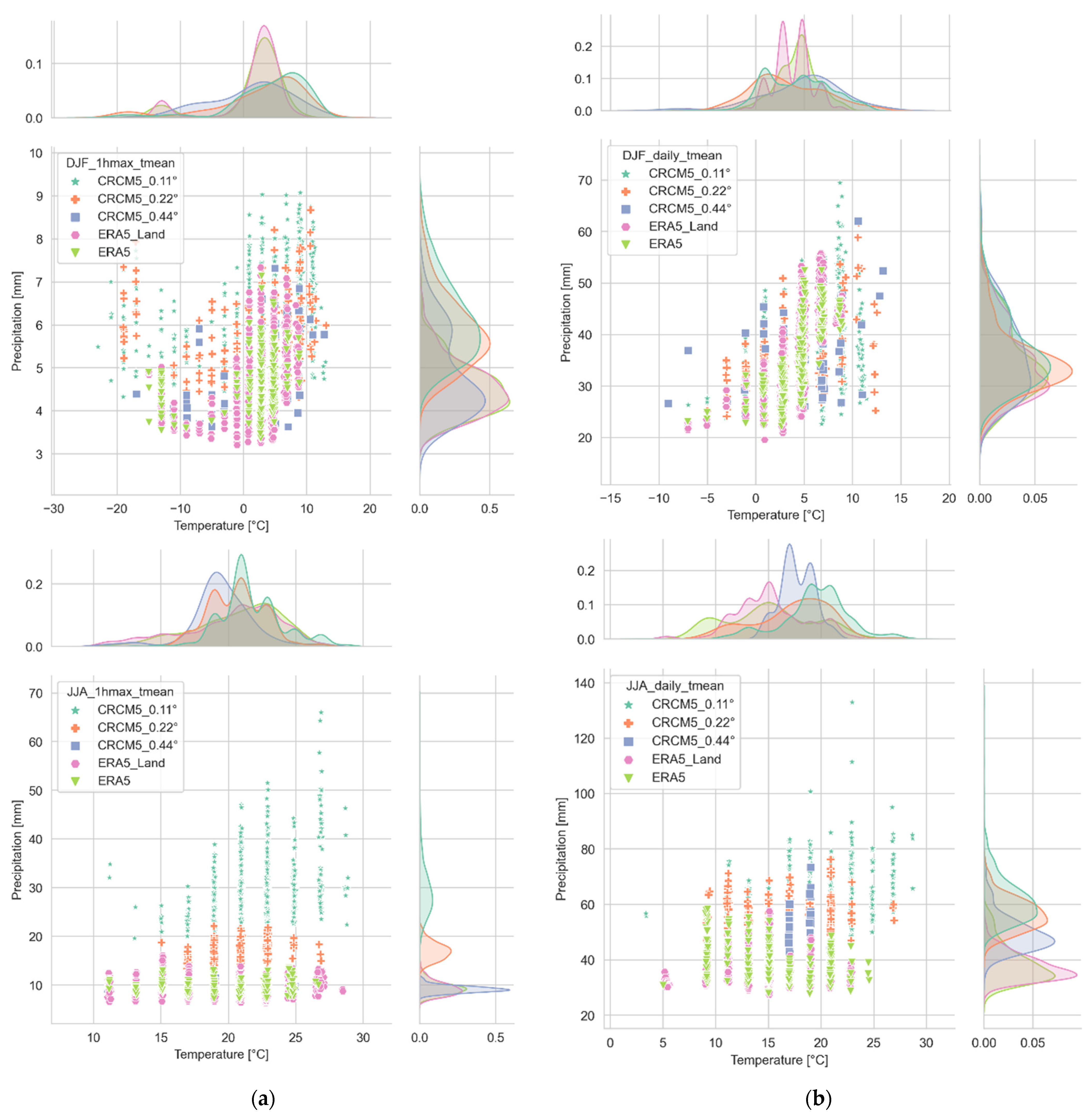
In Figure 4, the frequency distribution of the maximum values of the 99th percentile ( P 99 _ max) of hourly (a) and daily (b) precipitation is plotted on the vertical axis and the average temperature at which this value was reached on the horizontal axis. In other words, for each grid point and each dataset, the highest percentiles obtained were extracted along with their corresponding mean temperature. This allowed us to determine the most extreme values reached according to the increase in temperatures for each product within the ORB. We can notice that the most extreme hourly precipitations range between 15 and 25 °C (and with the higher resolution CRCM5_0.11°; Figure 4a), with a maximum frequency around 20 °C for all data, which corresponds to the hook shape identified earlier in Figure 2 for the CRCM5 simulations. In addition, the reanalyses generate a quite different behavior from the model simulations, with maximum precipitation values that do not exceed 15 mm/h even for the highest temperatures. This goes against what we observe in southern Québec, where daily or hourly extremes of rain are higher in summer or fall, when average temperatures are above 15 °C, than during the cold season (see climatological extremes at the Montréal station; [83,84]). A plausible explanation is that ERA5 reanalyses tend to underestimate the frequency of heavy precipitation events, especially in summer [85,86], whereas these reanalyses overestimate the occurrences of less intense precipitation [86]. A similar result was also observed for the daily extreme precipitation simulated by the CRCM5 model, where the P 99 _ max is reached for temperature values around 20 °C. However, the reanalyses show a more systematically different behavior. The P 99 _ max are slightly less intense than those of the CRCM5 simulations, with a frequency peak that shifts towards colder temperatures (around 10–15 °C) compared to the model (see Figure 4b). We can also note that the reanalysis ERA5-Land product generates slightly higher daily extreme precipitation than the parent reanalysis ERA5 model.

3.2. Spatial Distribution of the Scaling Factor α at the Annual Scale

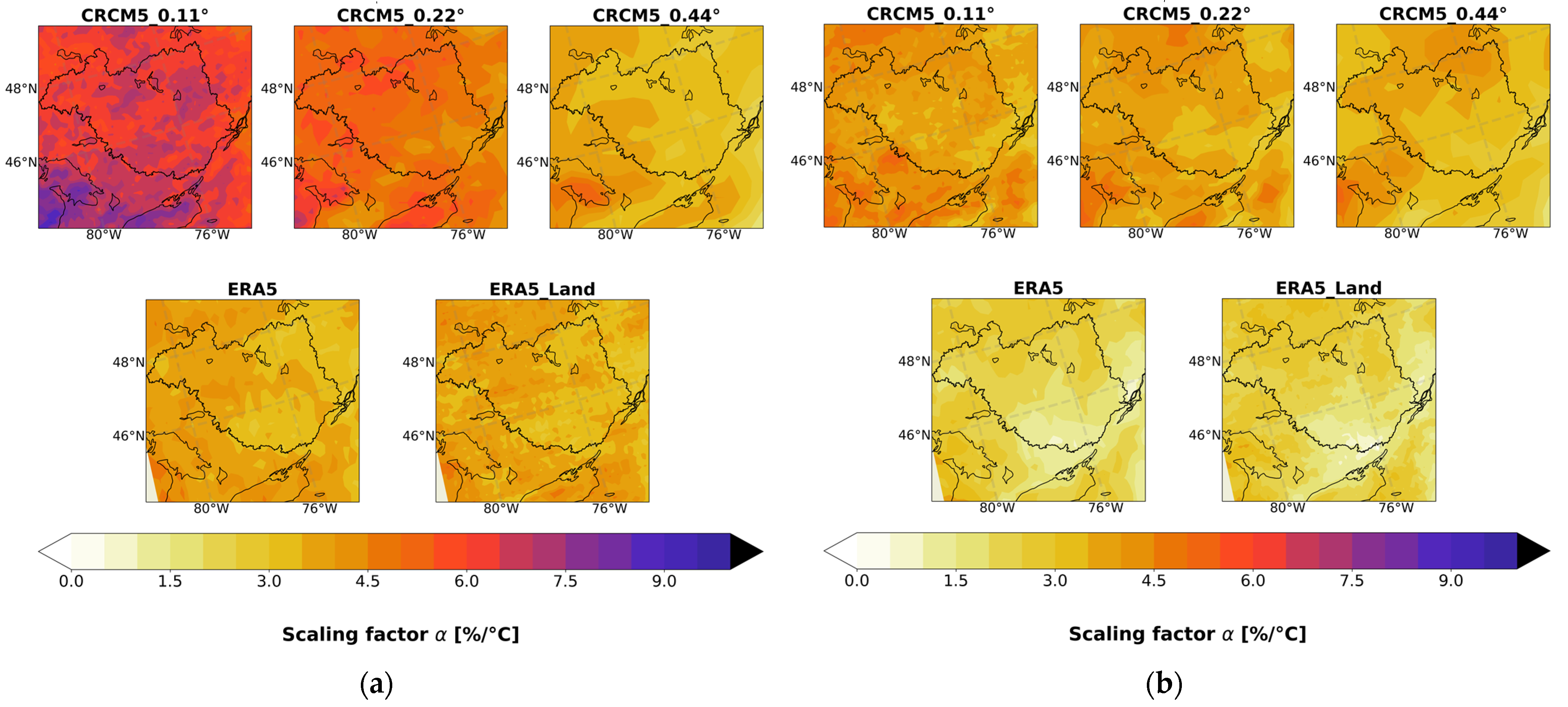
Figure 5 shows the spatial distribution of the scaling factor α obtained from the exponential regression (Equation (1)). For hourly precipitation, the difference between the scaling factor α obtained from the CRCM5_0.11° and the other data sources is quite remarkable, especially in the areas surrounding the Great Lakes, where α is super-CC.
This might suggest that the dependency between the hourly extreme precipitation and the temperature increases with the resolution, which plays a key role in capturing the well-known lake effects from higher precision in land–water boundary conditions within the CRCM5 (see the effects on higher precipitation values in [87]). In the case of daily precipitation, the scaling factor α is systematically sub-CC and less than 5.5%/°C. In Figure 5, the white regions in the southeast part of the domain indicate grid points where the level of statistical significance (5%, i.e., p-value ≤ 0.05) was not reached. This implies that there is no robust statistical relationship between extreme precipitation and mean temperature in this region of the domain for the lower resolution of the model and the reanalysis.

3.3. Seasonal Variability of the Scaling Factor α

As mentioned in Section 1, the seasonal variability of temperature and precipitation regimes is one of the main factors responsible for the variation in the CC scaling factor. Using the same methodology at the seasonal scale versus the one presented at the annual scale in the previous section, an analysis of the potential differences between extreme precipitation (hourly and daily) during winter and summer seasons is presented in the following paragraph.
In Figure 6, the evolution of the 99th percentile of hourly and daily precipitation is shown as a function of the mean daily temperature in winter (a) and summer (b) for the ORB (domain #2). During the winter season, the hourly extreme precipitation increases slightly with temperature (Figure 6a), but the slope is much less pronounced than in summer (Figure 6b), where the hook-shaped behavior is observed for the CRCM5_0.11° and the CRCM5_0.22°, followed by a slight increase in the first case.
This behavior is absent at 0.44° and for the reanalyses, where precipitation continues to increase with temperature and then just levels off. For daily precipitation, the same behavior is observed. The 99th percentile increases with temperature in winter, and a hook shape appears in summer for the CRCM5, but is also weakly present in the reanalyses. In this case, the slope is sub-CC, and the hook shape is less pronounced than for the hourly precipitation. In addition, the difference between products is lower during winter than in summer. Consequently, this seasonal analysis confirms that the behavior in the form of a hook is associated with the summer season, and depends on the resolution of the model.
Figure 7a reveals that the scaling factor α is systematically sub-CC in winter for the median and the interquartile range (IQR) values for hourly precipitation. The scaling factor is slightly higher for daily precipitation in all cases, which contrasts with the results obtained at the annual scale (see Figure 3). In the summer season (Figure 7b), α is sub-CC for the median and the IQR in the cases of the CRCM5_0.22°, the CRCM5_0.44°, and the reanalyses for hourly precipitation. However, at higher resolution (CRCM5_0.11°), the median and the IQR are close to the CC scale, or even super-CC, exceeding the rate of 10%/°. For daily precipitation, the median, the IQR, and 1.5 × IQR are negatives, except in the case of the IQR of the CRCM-0.44°. As opposed to winter (Figure 7a), all products in summer (Figure 7b) reveal a systematic higher scaling factor α for hourly precipitation than for daily precipitation.
In Figure 8, the frequency distribution of the maximum values ( P 99 _ max) of the 99th percentile of hourly and daily precipitation is presented for the winter and summer seasons. In winter (top panels), the hourly precipitation values barely exceed 10 mm/h for temperatures between −20 °C and 10 °C. Again, the maximum hourly extreme precipitation is consistently higher for the CRCM5_0.11° than for ERA5 reanalyses or for the simulation of the CRCM5 at lower resolutions. For daily extreme precipitation, the probability distributions vary between 20 and 70 mm/d for temperatures between −10 °C and 15 °C.
During the summer season (bottom panels), the intensities are significantly higher than in winter for hourly precipitation, up to more than 50 mm/h for temperatures between 10 and 25 °C, and a maximum frequency between 20 and 22 °C. For daily precipitation, the summer season has the highest maximum values, even exceeding 100 mm/d when temperatures are between 10 and 25 °C, and with maximum values around 20 °C for the CRCM5_0.11°. Here, the daily extreme precipitation values are obtained for lower temperatures in the case of ERA5 and ERA5-Land. These reanalysis products also tend to generate lower extreme hourly and daily precipitation, which diverge from the values observed in our regions (i.e., over southern Québec; see [83]) and from the high resolution of the CRCM5 simulations, as already mentioned.

3.4. Hook-Shaped Behavior in Summer: Dynamical Explanation

In the results presented above, the extreme hourly and daily precipitation is systematically more intense during the summer season. However, simulated data at finer resolutions show that above a temperature threshold of ~20 °C, extreme precipitation tends to decrease with temperature. This hook-shaped behavior should be associated with particular synoptic or dynamic situations [26]. The objective of this section is to assess the link between atmospheric conditions at the synoptic scale and the decrease in extreme precipitation for the highest temperatures observed during the summer season. Since the hook shape was more evident for high-resolution data, we only use the simulation of the CRCM5_0.11° in the following analysis. To identify these links, three different synoptic situations have been proposed according to the range of mean temperature simulated over domain #3 (see Figure 1), namely: (1) Situation A, where Tmean < 15 °C; Situation B, where Tmean 15 °C ≤ T ≤ 25 °C; and Situation C, where Tmean > 25 °C.

3.4.1. Situation A: Tmean < 15 °C

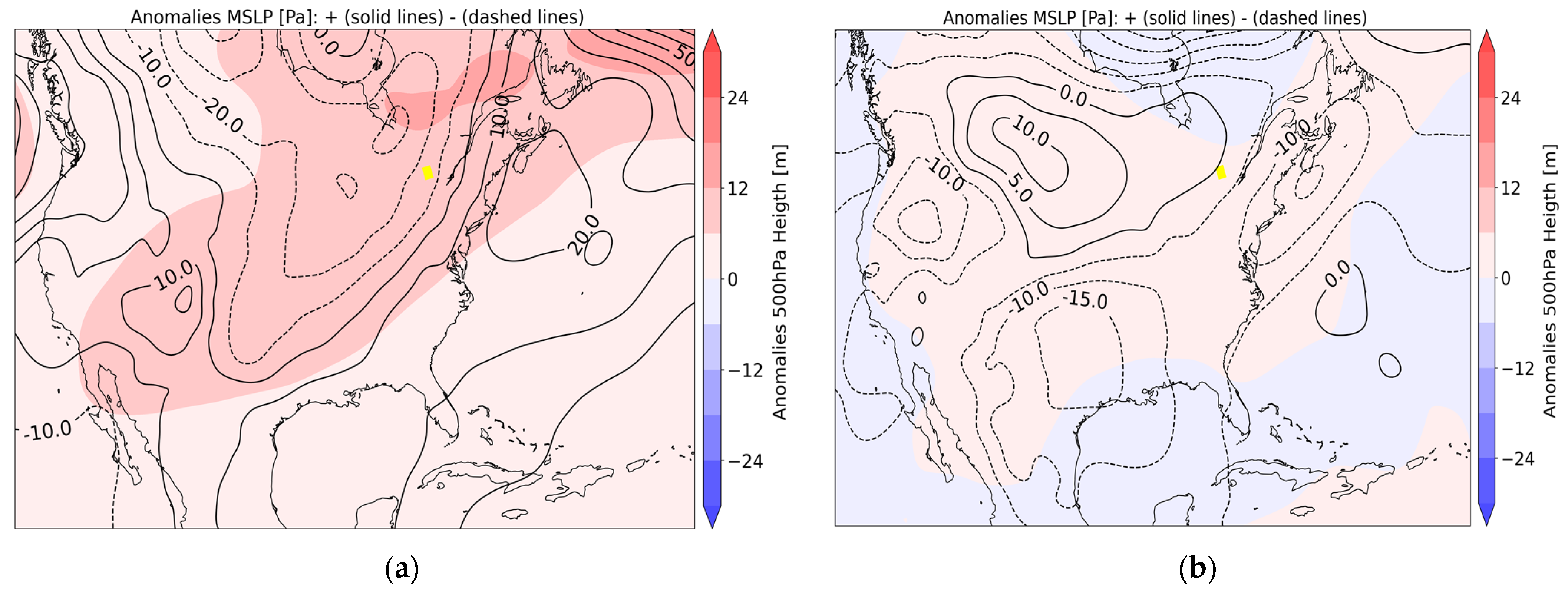
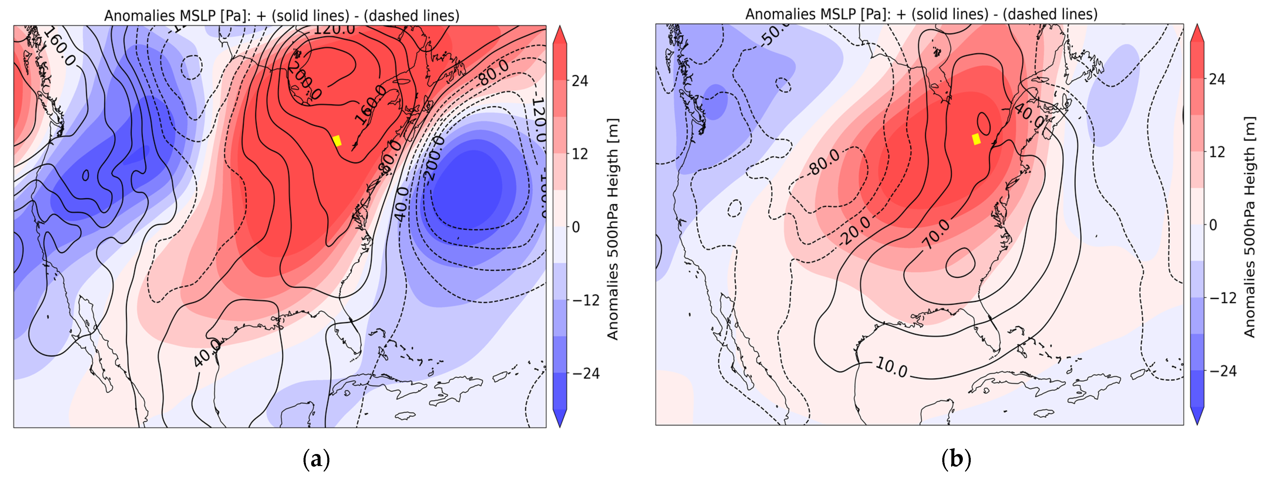
Figure 9 shows the MSLP and GZ-500 mean anomalies with respect to the 1981–2010 climatology, for the days where domain #3 had daily mean temperature records below 15 °C (seasonal temperatures colder than the 1981–2010 normal). The colors on the maps indicate the GZ-500 anomalies: in red, positive anomalies, and in blue, negative anomalies. Solid contour lines indicate positive MSLP anomalies, while dotted lines indicate negative MSLP anomalies. In all three months (June, July, and August), negative MSLP anomalies are observed within domain #3 and over all domains (#1 and #2, see Figure 1), with a low-pressure system deeper than normal to the east of the domain and positive MSLP anomalies to the west. In this configuration, more frequent depressions, or more intense than normal, seem to affect the east coast, increasing the probability of precipitation (occurrence and intensity, or even duration) in the study region.
For the three months, the anomalies of the GZ-500 are also negative over the region, which means a cooler-than-normal mid-troposphere, and therefore a potential instability favorable to upward motion and condensation of water vapor. In July, the GZ-500 pattern shows two positive anomalies and a negative anomaly above the region of interest. This means a cold shortwave trough at high altitude favorable to cyclogenesis and, therefore, to the occurrence of precipitation. In June and August, the situations are similar, although there is a more widespread negative anomaly of the GZ-500 in August over all of eastern Canada, including the Hudson Bay region. The physical mechanisms favorable to the occurrence of precipitation seem more associated with well-defined synoptic scale systems. Patterns associated with a 500 hPa trough and vertical wind shear will promote more frequent temperature advection and upward movements than normal. This is favorable to the creation of frontal zones or baroclinic zones associated with thermal contrasts between air masses of different origins favorable to the occurrence of precipitation.

3.4.2. Situation B: 15 °C ≤ Tmean ≤ 25 °C

Figure 10 corresponds to days when the daily mean temperature is between 15 and 25 °C (Situation B) in domain #3. Note that this situation corresponds to average temperature values close to normal seasonal climates in the study region. In this context, the MSLP and GZ-500 anomalies are less marked than in the previous case (Situation A) and are weak, in the order of −10 to 20 Pa and 6 to 12 m, respectively. The month of June presents a slightly lower MSLP than normal for the study region, and, unlike Situation A, a slightly warmer mid-troposphere with a positive GZ-500 anomaly. For the months of July and August, these anomalies in altitude persist, although less marked than during the month of June, since these are the months when the average temperature is most often between 20 and 22 °C in southern Québec. This situation is typically the synoptic and mesoscale conditions found in summer in southern Québec and corresponds to the highest rainfall occurrences and intensities, depending on the nature of the meteorological systems affecting the region (synoptic systems, frontal and mesoscale systems, and thunderstorm cells).

3.4.3. Situation C: Tmean > 25 °C

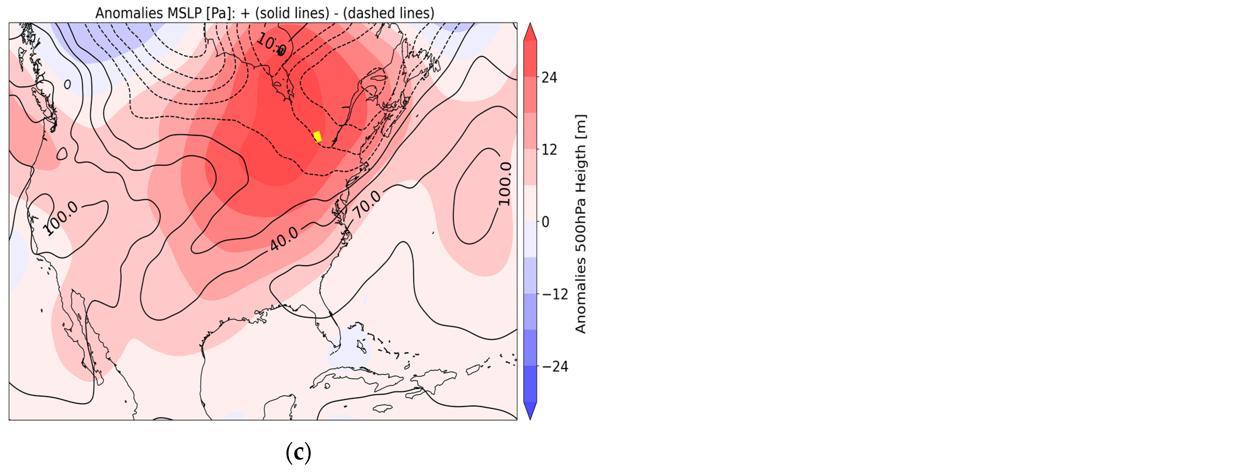
Situation C (Figure 11) corresponds to mean daily temperature values above the normal climate for this region. Unlike the previous cases, the hottest days show the strong positive anomalies of the GZ-500, corresponding to a warmer mid-troposphere than normal. This warm anomaly is greatest in June and more extended to the east and south in August. On the surface, strong positive anomalies of the MSLP are present in June and July (anticyclonic situation more frequent than normal), although with weak negative anomalies in August (weak depression or high pressure less marked than normal).
The positive anomalies mean that anticyclonic synoptic situations cover the region, characterized by sunny days (fewer occurrences of rain) and, therefore, warmer temperatures. These atmospheric conditions are most often accompanied by low relative humidity [28]. However, precipitation events can be intense with the occurrence of convective precipitation via thunderstorm systems, but less frequent. The decrease in the frequency of extreme events during warmer days in the summer season confirms the hook-like behavior observed in the region and explains the decrease in the 99th percentile with respect to previous B and C conditions, resulting in an inversion of the slope after the breaking point (i.e., around 20–22 °C).

3.5. Behavior of the CC Scaling Factor from the Highest Resolution (CRCM6/GEM5 Simulation)

In this section, the CRCM6/GEM5 (CP) simulation at 2.5 km of resolution is analyzed in order to evaluate whether the behavior described previously, i.e., an inflection point beyond 20 °C and the super-CC behavior for the high-resolution simulation, is also observed. However, as the CRCM6/GEM5 simulations only cover a short period (7 years between 2015 and 2021), which is different from the sample size of the data analyzed in the previous sections (30 years over the 1981–2010 period), no definitive conclusion can be drawn from the results obtained here.
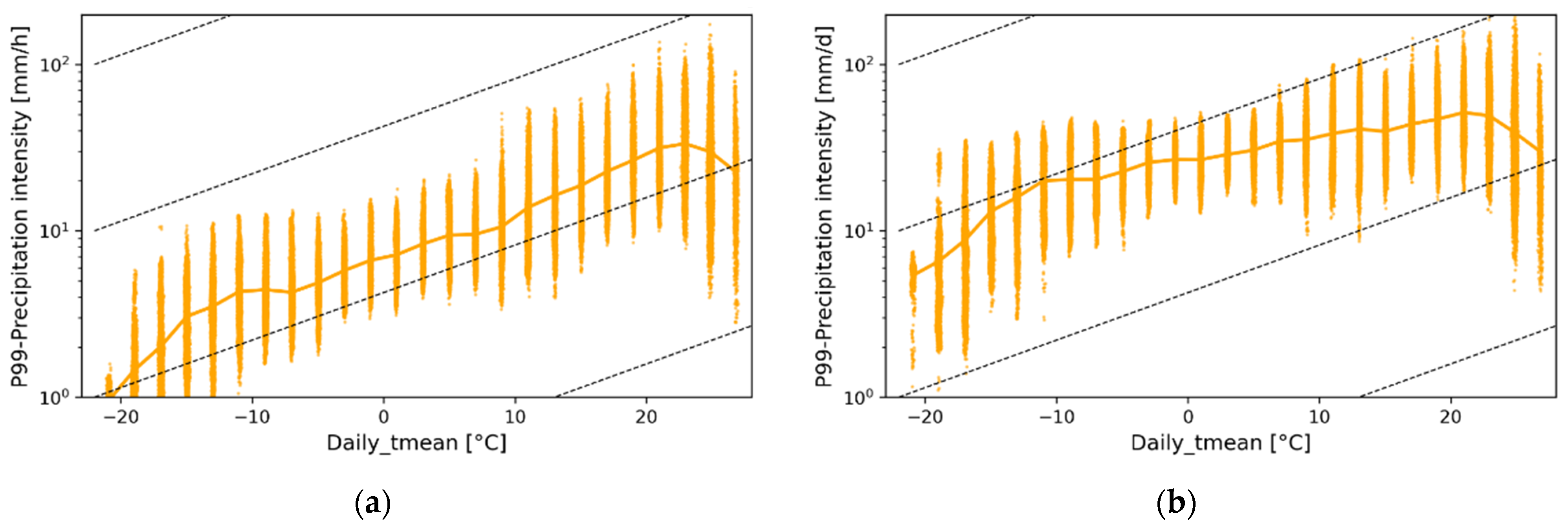
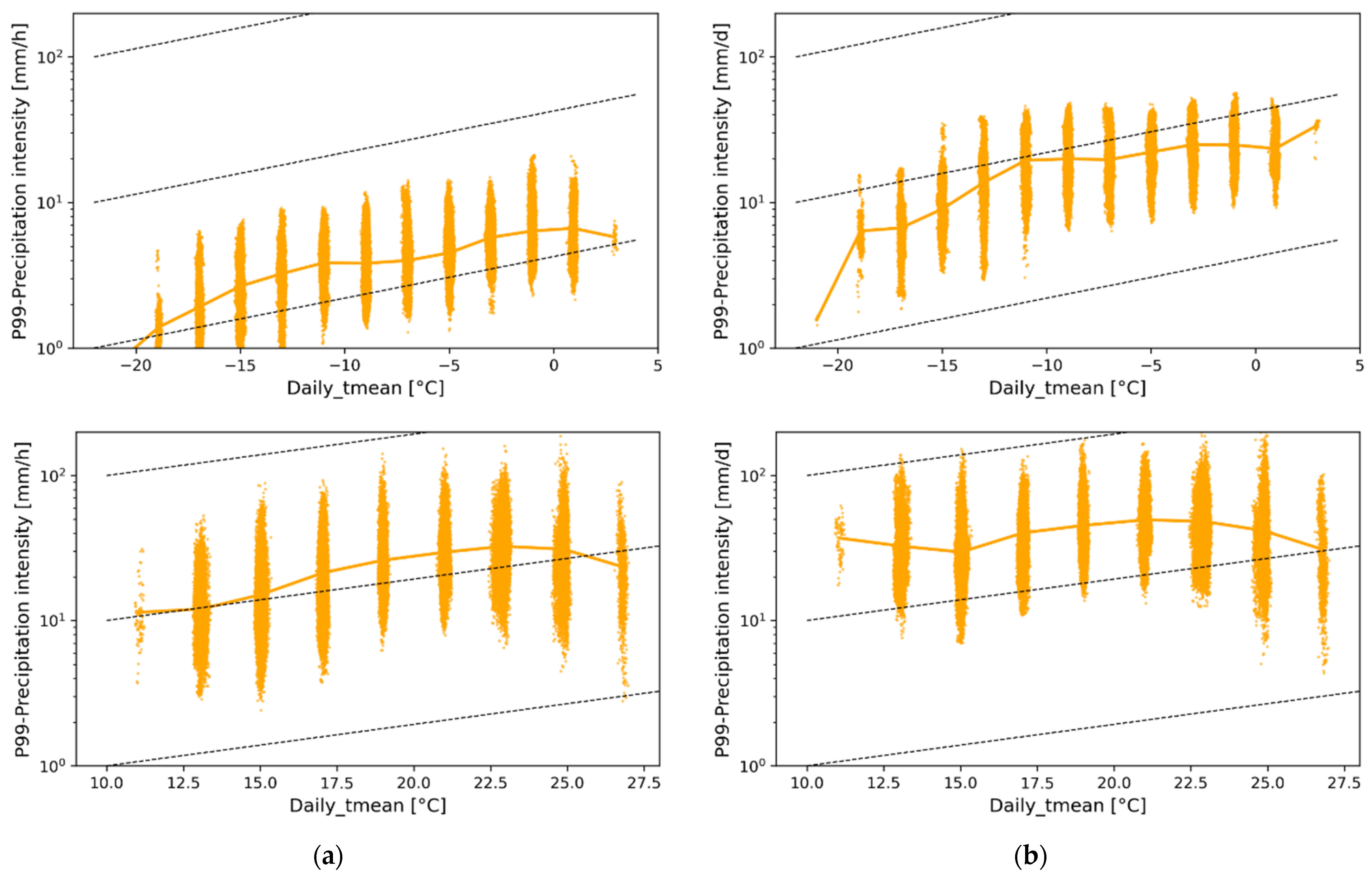
Figure 12 presents the evolution of the 99th percentile of (a) hourly and (b) daily precipitation as a function of mean temperature for domain #2 (presented in Figure 1). As described in Section 2.2, the CRCM6/GEM5 simulation used in our study is at a very high spatial resolution (2.5 km) and the deep convection is explicit, unlike the simulations of the CRCM5. Similar to the results shown with the fifth version of the model (CRCM5_0.11°), extreme hourly precipitation increases more rapidly with temperature than daily precipitation, and the slope is always less pronounced for daily precipitation. In general, the rate of change in hourly extreme precipitation is higher for all temperature ranges below 20 °C in the CRCM6/GEM5 (Figure 12a) than in the CRCM5 (whatever the resolution, see Figure 2). The hook-shaped behavior (inflection point around 20–22 °C) is also present here in both hourly and daily cases, but is more pronounced for hourly than for daily precipitation, as noted previously.
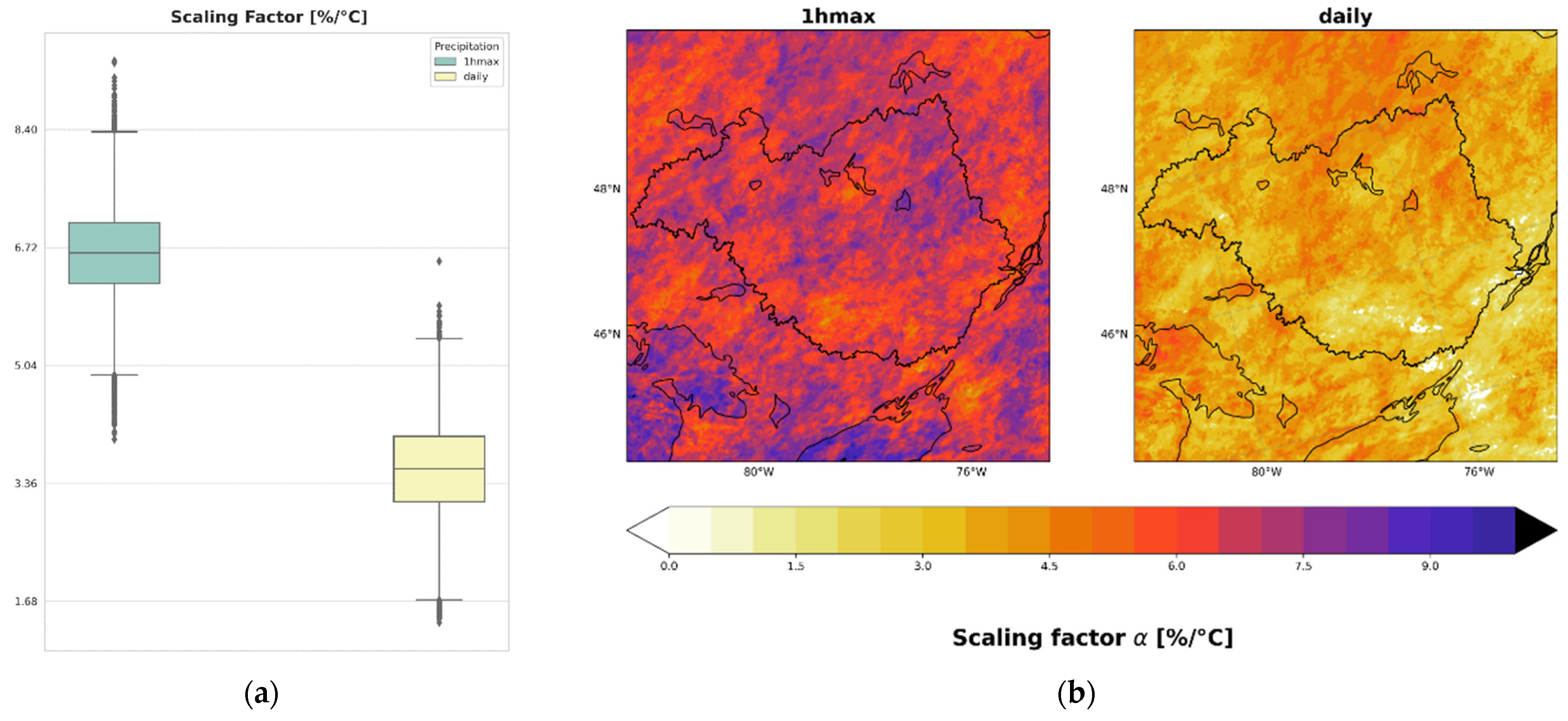
The scaling factor α (presented in Figure 13a) is close to the rate of the change in CC for hourly precipitation, but it is still lower than the rate of change in the CC for daily precipitation. Figure 13b shows the spatial distribution of the scaling factor α obtained from the exponential regression. For hourly precipitation, α is, in general, super-CC, while for daily precipitation, α is systematically sub-CC and less than 5.5%/°C.
This confirms, once again, the dependency between the hourly extreme precipitation and the temperature increases with the resolution. We can also note that this highest resolution (CRCM6/GEM5 at 2.5 km) seems to generate a higher scaling factor (i.e., the highest CC values) for hourly extreme precipitation than the lower CRCM5_0.11° resolution (see Figure 3 vs. Figure 13a), as noted in recent studies (i.e., the magnitude of extreme precipitation varies with the spatial resolution of models (see [88,89])).
Figure 14 presents the evolution of the 99th percentile of (a) maximum hourly precipitation (1 hmax) and (b) daily precipitation as a function of the daily mean temperature for the winter and summer seasons. The hourly extreme precipitation is much more intense in the summer season, and the hook shape is present here for daily and hourly precipitation (around 22.5–25 °C). In winter, although a small inflection is observed, hourly and daily precipitation tends to increase with temperature. In both seasons and temporal scales, the higher resolution (CRCM6/GEM5 at 2.5 km) more often generates higher extreme precipitation values than at a lower resolution (i.e., CRCM5 as shown in Figure 6).

4. Conclusions

The general objective of this research was to determine the applicability of the CC relationship using the CRCM model (versions 5 and 6) at different resolutions and the ERA5 and ERA5-Land reanalysis in the ORB (Canada). The results obtained allowed us to identify three factors, already proposed in previous studies, that play a fundamental role in the applicability of the CC relationship at the regional scale. These three factors are: the temporal scale chosen for the analysis, the resolution of the simulated or reanalyzed data, and the season of the year. That said, it can be concluded that for the study area:
  • The daily precipitation follows a rate of change lower than the CC scaling factor, while hourly precipitation increases more rapidly with temperature, demonstrating the importance of timescale in the studies that address the CC relation.
  • For the CRCM5 simulations at higher spatial resolution (0.11°), the rates of change obtained were higher than the CC rate of 6.8%/°C, even 10.2%/°C for hourly extreme precipitation, also known as super-CC.
  • The added value of the high resolution of the model seems quite substantial, although it needs to be validated with reliable observed hourly (or sub-hourly) data. The use of higher resolution models allows a better spatial representation of the precipitation events on a seasonal scale, especially for events of a convective nature.
  • For the CRCM5 simulations, hourly and daily precipitation increases with temperature up to a threshold of around 20–22 °C, and then it decreases. This hook-shaped behavior was not identified with the reanalysis data, which seem to systematically underestimate the most intense precipitation events, and the relation was always sub-CC in such a case, even for hourly precipitation.
  • For the winter season, the extreme precipitation shows a slight increase in temperature, while the summer period is associated with the hook behavior.
  • The moisture-holding capacity of the atmosphere, described from the CC equation, is the dominant factor for temperatures up to 20 °C, but not necessarily above this threshold, when it is essential to take into account other factors, such as the availability of humidity at the time of the precipitation event in relation to the water-holding capacity of the atmosphere. The presence of dynamic mechanisms that promote upward vertical motions and provide the cooling needed to produce saturation is also a key factor to consider, as noted in previous studies.
  • Using the average daily temperature instead of the temperature at the time of the precipitation event can have a non-negligible effect on the peak of the frequency distribution of the maximum percentile of precipitation (P99_max).
  • For the CRCM6 simulation at higher resolution (2.5 km), the rate of change, on average, was close to the relationship of CC for hourly precipitation and sub-CC for daily precipitation. Regarding the intra-seasonal analysis, the results were also similar to those of the CRCM5 (0.11°), but with slightly higher magnitude or extreme precipitations for the finer scale model.
Even if our analysis included seven years of simulations of the sixth version of the CRCM, still under development at the ESCER center, it is extremely important to continue documenting extreme events at very high spatial resolution for longer periods and for other regions. In this and ongoing simulations where deep convection can be explicit, extreme precipitation is potentially better represented, more understandable, and more predictable than with convection-parameterized models (see [88]).
One of the findings of our study is the hook-shaped behavior observed in the summer season associated with anticyclonic synoptic situations and low relative humidity levels. Potential avenues for future research could be to develop more insights into the role of the compounding behavior of extreme hourly rainfall immediately following a heatwave (both events expected to become more frequent in the future), as already found in [89] for temperate or colder climates. As explained by Sauter et al. [90], compared with isolated hazards, compound events can lead to higher economic losses and death tolls [91]. Future research should also identify and evaluate whether these anticyclonic synoptic conditions are linked to atmospheric blocking events that generate prolonged periods of very high temperatures (heatwaves), often amplified by soil moisture deficits [92]. These avenues for future research are requisite because compound effects in the atmospheric circulation changes under global warming can generate high-impact weather conditions, as exemplified over Europe, where circulation changes modulate extreme events already in the present climate [8].
Our results demonstrated the limitations of using reanalysis data for extreme precipitation studies. Unfortunately, the lack of a sufficiently reliable hourly weather station in the study area did not allow a comparison between the data simulated by the model and other products other than the reanalyses. The global precipitation product MSWEP V2.8 [93], available via the GloH20 website (http://www.gloh2o.org/mswep/, accessed on 26 October 2021), with a three-hourly 0.1° resolution was also used to calculate the 99th percentile of daily precipitation. The results obtained were similar to those of the ERA5 data and can be consulted in [94]. However, products could be used such as the observational Integrated Multi-satellite Retrievals for Global Precipitation (IMERG, Final Run version 6; [95]) are available at 0.1° resolution for half-hourly precipitation data. These last datasets were recently used to evaluate the causes for the negative scaling of extreme precipitation with high temperatures over various regions of the globe [89].
Our study also suggests continuing the research of the applicability of the CC relationship in other climatic zones across Canada to better understand the impact of local effects in CC scaling, especially for the hourly timescale. It is important to remember that the availability of humidity in the atmosphere can vary considerably from one region or season to another (see, for example, the recent studies of [20,89,96,97]). Further study also needs to be carried out over the ORB region, particularly after the persistence of warm days or heatwaves, as the recent study of Sauter et al. [90] has shown that compound extreme hourly rainfall can be preconditioned by heatwaves occurring over mid-latitudes.
Finally, it would be relevant to assess the “projected” scaling for different climate change scenarios and for CRCM6/GEM5 (convection-permitting) resolutions. This could have a significant impact on how to assess the risk of flooding in the future. It will be greatly influenced by the rapid and irreversible increase in temperature and the associated modification of extreme precipitation events (see [22,23,24]) that are affected by the spatial resolution of climate models, as higher-resolution models produce more intense precipitation and reduced wet-hour frequency compared to coarse resolution models (see [88]). Indeed, historic flooding in recent years across the province of Québec constitutes a major concern with a clear link with the increase in precipitation extremes in spring [7], as temperatures are rising faster in Canada than the global average [98].

Author Contributions

Conceptualization, A.L. and P.G.; methodology, A.L. and P.G.; software, A.L.; validation, P.G. and R.L.; formal analysis, A.L., P.G., and R.L.; investigation, A.L.; resources, P.G.; writing—original draft preparation, A.L.; writing—review and editing, A.L., P.G., and R.L.; visualization, A.L.; supervision, P.G. and R.L.; project administration, P.G.; funding acquisition, P.G. All authors have read and agreed to the published version of the manuscript.

Funding

This work was supported by the Discovery Grant program of the Natural Sciences and Engineering Research Council of Canada (NSERC) under grants 2016-06436 and 2022-05032, by the strategic research chair of UQAM held by Pr. Philippe Gachon, and by the scholarship for the exemption of additional tuition fees for foreign students from UQAM.

Institutional Review Board Statement

Not applicable.

Informed Consent Statement

Not applicable.

Data Availability Statement

The CRCM5 simulations are available through the North-American CORDEX Program and its portal (see https://na-cordex.org/na-cordex-on-aws.html; accessed on 11 March 2021). A copy of the NA-CORDEX dataset is also available on Amazon Web Services (AWS, see https://registry.opendata.aws/ncar-na-cordex/). We thank the AWS Open Data Sponsorship Program and the Amazon Sustainability Data Initiative for providing free storage and egress for these data. The ERA5 and ERA5-Land are products of the reanalysis developed by ECMWF are available to the public through the Climate Data Store of Copernicus (see cds.climate.copernicus.eu/#!/home; accessed on 21 March 2022). We thank Copernicus for the access of these data products. The CRCM6/GEM5 simulations is not yet available, but will be openly available in Borealis, the Canadian Dataverse Repository, using longer time windows when a complete evaluation of available simulations will be finalized.

Acknowledgments

Computations were made on the supercomputers, managed by Calcul Québec and the Digital Research Alliance of Canada, whose operation is funded by the Canada Foundation for Innovation, Ministère de l’Économie et de l’Innovation du Québec (MEI) and the Fonds de recherche du Québec-Nature et technologies (FRQNT). The help of Katja Winger and François Roberge of the ESCER center, who are responsible for maintaining the CRCM model versions as well as carrying out CRCM simulations, is also strongly acknowledged. Computations to produce the CRCM6 (CRCM5) simulations were made on the supercomputer Narval (Beluga), managed by the Digital Research Alliance of Canada (https://alliancecan.ca/en).

Conflicts of Interest

The authors declare no conflict of interest. The funders had no role in the design of the study; in the collection, analyses, or interpretation of data; in the writing of the manuscript; or in the decision to publish the results.

References

  1. Schroeer, K.; Kirchengast, G. Sensitivity of extreme precipitation to temperature: The variability of scaling factors from a regional to local perspective. Clim. Dyn. 2017, 50, 3981–3994. [Google Scholar] [CrossRef] [Green Version]
  2. Elahi, E.; Khalid, Z.; Tauni, M.Z.; Zhang, H.; Lirong, X. Extreme weather events risk to crop-production and the adaptation of innovative management strategies to mitigate the risk: A retrospective survey of rural Punjab, Pakistan. Technovation 2022, 117, 102255. [Google Scholar] [CrossRef]
  3. Wijeratne, V.P.I.S.; Li, G.; Mehmood, M.S.; Abbas, A. Assessing the Impact of Long-Term ENSO, SST, and IOD Dynamics on Extreme Hydrological Events (EHEs) in the Kelani River Basin (KRB), Sri Lanka. Atmosphere 2022, 14, 79. [Google Scholar] [CrossRef]
  4. Wallemacq, P. Economic Losses, Poverty & Disasters: 1998–2017; Centre for Research on the Epidemiology of Disasters, CRED: Brussels, Belgium, 2018; 30p. [Google Scholar]
  5. WMO. Atlas of Mortality and Economic Losses from Weather, Climate and Water Extremes (1970–2019); WMO-No. 1267; WMO: Geneva, Switzerland, 2021; 90p. [Google Scholar]
  6. Poitras, V. Étude des Débits des Cours d’eau Canadiens Dans un Climat Changeant Université du Québec à Montréal. WorldCat.org. Montréal. 2010. Available online: https://central.bac-lac.gc.ca/.item?id=TC-QMUQ-3592&op=pdf&app=Library (accessed on 23 April 2021).
  7. Benoit, C.; Demers, I.; Roberge, F.; Gachon, P.; et Laprise, R. Inondations des Printemps 2017 et 2019 Dans le Bassin Versant de la Rivière des Outaouais (Québec, Canada): Analyse des Facteurs Physiographiques et Météorologiques en Cause; Buffin-Bélanger, T., Maltais, D., Mario, M., Eds.; Les inondations au Québec: Risques, aménagement du territoire, impacts socioéconomiques et transformation des vulnérabilités; Presse de l’Université du Québec: Québec City, QC, Canada, 2022; pp. 29–58. [Google Scholar]
  8. Trenberth, K.E. Changes in precipitation with climate change. Clim. Res. 2011, 47, 123–138. [Google Scholar] [CrossRef] [Green Version]
  9. Bonsal, B.R.; Peters, D.L.; Seglenieks, F.R.A.; Berg, A. Changes in Freshwater Availability across Canada; Chapter 6 in Canada’s Changing Climate Report; Bush, E., Lemmen, D.S., Eds.; Government of Canada: Ottawa, ON, Canada, 2019; pp. 261–342. [Google Scholar]
  10. Bonsal, B.R.; Dibike, Y.B.; Peters, D.L.; Shrestha, R.R. Special Issue: Past and Future Trends and Variability in Hydro-Climatic Processes. Water 2021, 13, 2199. [Google Scholar] [CrossRef]
  11. INSPQ. Événements Météorologiques Extrêmes. 2020. Available online: http://www.monclimatmasante.qc.ca/%C3%A9v%C3%A9nements-extr%C3%AAmes.aspx#:~:text=Les%20inondations%20%3A%20Au%20Qu%C3%A9bec%2C%20les,indirects%20sur%20les%20populations%20et (accessed on 15 June 2022).
  12. Drobinski, P.; Da Silva, N.; Panthou, G.; Bastin, S.; Muller, C.; Ahrens, B.; Borga, M.; Conte, D.; Fosser, G.; Giorgi, F.; et al. Scaling precipitation extremes with temperature in the Mediterranean: Past climate assessment and projection in anthropogenic scenarios. Clim. Dyn. 2016, 51, 1237–1257. [Google Scholar] [CrossRef] [Green Version]
  13. Lenderink, G.; van Meijgaard, E. Increase in hourly precipitation extremes beyond expectations from temperature changes. Nat. Geosci. 2008, 1, 511–514. [Google Scholar] [CrossRef]
  14. Jones, R.H.; Westra, S.; Sharma, A. Observed relationships between extreme sub-daily precipitation, surface temperature, and relative humidity. Geophys. Res. Lett. 2010, 37, L22805. [Google Scholar] [CrossRef] [Green Version]
  15. Utsumi, N.; Seto, S.; Kanae, S.; Maeda, E.E.; Oki, T. Does higher surface temperature intensify extreme precipitation? Geophys. Res. Lett. 2011, 38. [Google Scholar] [CrossRef]
  16. Trenberth, K.E. Conceptual Framework for Changes of Extremes of the Hydrological Cycle with Climate Change. Clim. Chang. 1999, 42, 327–339. [Google Scholar] [CrossRef]
  17. Allen, M.R.; Ingram, W.J. Constraints on future changes in climate and the hydrologic cycle. Nature 2002, 419, 224–232. [Google Scholar] [CrossRef] [PubMed]
  18. Emori, S.; Brown, S.J. Dynamic and thermodynamic changes in mean and extreme precipitation under changed climate. Geophys. Res. Lett. 2005, 32. [Google Scholar] [CrossRef]
  19. Pall, P.; Allen, M.R.; Stone, D.A. Testing the Clausius–Clapeyron constraint on changes in extreme precipitation under CO2 warming. Clim. Dyn. 2006, 28, 351–363. [Google Scholar] [CrossRef]
  20. Magan, B.; Kim, S.; Wasko, C.; Barbero, R.; Moron, V.; Nathan, R.; Sharma, A. Impact of atmospheric circulation on the rainfall-temperature relationship in Australia. Environ. Res. Lett. 2020, 15, 094098. [Google Scholar] [CrossRef]
  21. WMO. State of the Global Climate 2021. 2022. Available online: https://library.wmo.int/doc_num.php?explnum_id=11178 (accessed on 13 August 2022).
  22. IPCC. Climate Change 2021: The Physical Science Basis. Contribution of Working Group I to the Sixth Assessment Report of the Intergovernmental Panel on Climate Change; Masson-Delmotte, V., Zhai, A.P., Pirani, S.L., Connors, C., Péan, S., Berger, N., Caud, Y., Chen, L., Goldfarb, M.I., Gomis, M., et al., Eds.; Cambridge University Press: Cambridge, UK; New York, NY, USA, 2021. [Google Scholar] [CrossRef]
  23. IPCC. Climate Change 2013: The Physical Science Basis. Contribution of Working Group I to the Fifth Assessment Report of the Intergovernmental Panel on Climate Change; Stocker, T.F., Qin, G.-K.D., Plattner, M., Tignor, S.K., Allen, J., Boschung, A., Nauels, Y., Xia, V.B., Midgley, P.M., Eds.; Cambridge University Press: Cambridge, UK; New York, NY, USA, 2013; 1535p. [Google Scholar] [CrossRef] [Green Version]
  24. IPCC. Global Warming of 1.5 °C. In An IPCC Special Report on the Impacts of Global Warming of 1.5 °C above Pre-Industrial Levels and Related Global Greenhouse Gas Emission Pathways, in the Context of Strengthening the Global Response to the Threat of Climate Change, Sustainable Development, and Efforts to Eradicate Poverty; Masson-Delmotte, P.V., Zhai, H.O., Pörtner, D., Roberts, J., Skea, P.R., Shukla, A., Pirani, W., Moufouma-Okia, C., Péan, R., Pidcock, S., et al., Eds.; IPCC: Geneva, Switzerland, 2018; In Press. [Google Scholar]
  25. Groisman, P.Y.; Knight, R.W.; Easterling, D.R.; Karl, T.R.; Hegerl, G.C.; Razuvaev, V.N. Trends in Intense Precipitation in the Climate Record. J. Clim. 2005, 18, 1326–1350. [Google Scholar] [CrossRef]
  26. Westra, S.J.; Fowler, H.J.; Evans, J.P.; Alexander, L.V.; Berg, P.R.; Johnson, F.; Kendon, E.J.; Lenderink, G.; Roberts, N.M. Future changes to the intensity and frequency of short-duration extreme rainfall. Rev. Geophys. 2014, 52, 522–555. [Google Scholar] [CrossRef] [Green Version]
  27. Haerter, J.O.; Berg, P.; Hagemann, S. Heavy rain intensity distributions on varying time scales and at different temperatures. J. Geophys. Res. Atmos. 2010, 115. [Google Scholar] [CrossRef]
  28. Lenderink, G.; Mok, H.Y.; Lee, T.C.; van Oldenborgh, G.J. Scaling and trends of hourly precipitation extremes in two different climate zones—Hong Kong and the Netherlands. Hydrol. Earth Syst. Sci. 2011, 15, 3033–3041. [Google Scholar] [CrossRef] [Green Version]
  29. Panthou, G.; Mailhot, A.; Laurence, E.; Talbot, G. Relationship between Surface Temperature and Extreme Rainfalls: A Multi-Time-Scale and Event-Based Analysis. J. Hydrometeorol. 2014, 15, 1999–2011. [Google Scholar] [CrossRef]
  30. Haerter, J.O.; Berg, P. Unexpected rise in extreme precipitation caused by a shift in rain type? Nat. Geosci. 2009, 2, 372–373. [Google Scholar]
  31. Shaw, S.B.; Royem, A.A.; Riha, S.J. The Relationship between Extreme Hourly Precipitation and Surface Temperature in Different Hydroclimatic Regions of the United States. J. Hydrometeorol. 2011, 12, 319–325. [Google Scholar] [CrossRef]
  32. Mishra, V.; Wallace, J.M.; Lettenmaier, D.P. Relationship between hourly extreme precipitation and local air temperature in the United States. Geophys. Res. Lett. 2012, 39. [Google Scholar] [CrossRef]
  33. Dai, A.; Trenberth, K.E.; Karl, T.R. Effects of clouds, soil moisture, precipitation, and water vapor on diurnal temperature range. J. Clim. 1999, 12, 2451–2473. [Google Scholar] [CrossRef]
  34. Zhao, W.; Khalil, M.A.K. The Relationship between Precipitation and Temperature over the Contiguous United States. J. Clim. 1993, 6, 1232–1236. [Google Scholar] [CrossRef]
  35. Vautard, R.; Yiou, P.; D’Andrea, F.; de Noblet, N.; Viovy, N.; Cassou, C.; Polcher, J.; Ciais, P.; Kageyama, M.; Fan, Y. Summertime European heat and drought waves induced by wintertime Mediterranean rainfall deficit. Geophys. Res. Lett. 2007, 34. [Google Scholar] [CrossRef] [Green Version]
  36. Wazneh, H.; Arain, M.A.; Coulibaly, P.; Gachon, P. Evaluating the Dependence between Temperature and Precipitation to Better Estimate the Risks of Concurrent Extreme Weather Events. Adv. Meteorol. 2020, 8763631. [Google Scholar] [CrossRef]
  37. Trenberth, K.E.; Shea, D.J. Relationships between precipitation and surface temperature. Geophys. Res. Lett. 2005, 32. [Google Scholar] [CrossRef]
  38. Trenberth, K.E.; Dai, A.; Rasmussen, R.M.; Parsons, D.B. The changing character of precipitation. Bull. Am. Meteorol. Soc. 2003, 84, 1205–1218. [Google Scholar] [CrossRef]
  39. D’Orgeville, M.; Peltier, W.R.; Erler, A.R.; Gula, J. Climate change impacts on Great Lakes Basin precipitation extremes. J. Geophys. Res. Atmos. 2014, 119, 10799–10812. [Google Scholar] [CrossRef]
  40. Drobinski, P.; Alonzo, B.; Bastin, S.; Silva, N.D.; Muller, C. Scaling of precipitation extremes with temperature in the French Mediterranean region: What explains the hook shape? J. Geophys. Res. Atmos. 2016, 121, 3100–3119. [Google Scholar]
  41. Cannon, A.J.; Innocenti, S. Projected intensification of sub-daily and daily rainfall extremes in convection-permitting climate model simulations over North America: Implications for future intensity duration–frequency curves. Nat. Hazards Earth Syst. Sci. 2019, 19, 421–440. [Google Scholar] [CrossRef] [Green Version]
  42. Oh, S.-G.; Sushama, L. Short-duration precipitation extremes over Canada in a warmer climate. Clim. Dyn. 2020, 54, 2493–2509. [Google Scholar] [CrossRef]
  43. Berthou, S.; Kendon, E.J.; Chan, S.C.; Ban, N.; Leutwyler, D.; Schär, C.; Fosser, G. Pan-European climate at convection-permitting scale: A model intercomparison study. Clim. Dyn. 2018, 55, 35–59. [Google Scholar] [CrossRef] [Green Version]
  44. Prein, A.F.; Rasmussen, R.M.; Ikeda, K.; Liu, C.; Clark, M.P.; Holland, G.J. The future intensification of hourly precipitation extremes. Nat. Clim. Chang. 2017, 7, 48–52. [Google Scholar] [CrossRef]
  45. Knist, S.; Goergen, K.; Simmer, C. Evaluation and projected changes of precipitation statistics in convection-permitting WRF climate simulations over Central Europe. Clim. Dyn. 2020, 55, 325–341. [Google Scholar] [CrossRef] [Green Version]
  46. Lenderink, G.; de Vries, H.; Fowler, H.J.; Barbero, R.; van Ulft, B.; van Meijgaard, E. Scaling and responses of extreme hourly precipitation in three climate experiments with a convection-permitting model. Philos. Trans. R. Soc. A 2021, 379, 20190544. [Google Scholar] [CrossRef]
  47. Fosser, G.; Adinolfi, M.; Ban, N.; Belušić, D.; Caillaud, C.; Cardoso, R.M.; Coppola, E.; Demory, M.-E.; De Vries, H.; Dobler, A. Convection-permitting climate models Offer More Certain Extreme Rainfall Projections. In Proceedings of the Copernicus Meetings, EGU General Assembly, Vienna, Austria, 23–27 May 2022; p. EGU22-7679. [Google Scholar] [CrossRef]
  48. Luu, L.N.; Vautard, R.; Yiou, P.; Soubeyroux, J.-M. Evaluation of convection-permitting extreme precipitation simulations for the south of France. Earth Syst. Dyn. 2022, 13, 687–702. [Google Scholar] [CrossRef]
  49. Cong, R.-G.; Brady, M. The Interdependence between Rainfall and Temperature: Copula Analyses. Sci. World J. 2012, 2012, 405675. [Google Scholar] [CrossRef] [Green Version]
  50. ECCC. Rapport de Données Quotidiennes Pour Juin 2021. 2022. Available online: https://climat.meteo.gc.ca/climate_data/daily_data_f.html?hlyRange=1994-02-01%7C2023-07-02&dlyRange=1994-07-26%7C2023-07-01&mlyRange=%7C&StationID=10868&Prov=QC&urlExtension=_f.html&searchType=stnName&optLimit=yearRange&Star-tYear=1840&EndYear=2023&selRowPerPage=25&Line=0&searchMethod=contains&txtStationName=st-jovite&timeframe=2&Day=2&Year=2021&Month=6# (accessed on 17 June 2022).
  51. Aleshina, M.; Semenov, V.A.; Chernokulsky, A.V. A link between surface air temperature and extreme precipitation over Russia from station and reanalysis data. Environ. Res. Lett. 2021, 16, 105004. [Google Scholar] [CrossRef]
  52. Ali, H.; Fowler, H.J.; Pritchard, D.; Lenderink, G.; Blenkinsop, S.; Lewis, E. Towards Quantifying the Uncertainty in Estimating Observed Scaling Rates. Geophys. Res. Lett. 2022, 49, e2022GL099138. [Google Scholar] [CrossRef] [PubMed]
  53. Aleshina, M.; Semenov, V. Observed extreme precipitation-temperature scaling in Russia during 1961–2017. In Proceedings of the 26th International Symposium on Atmospheric and Ocean Optics, Atmospheric Physics, Moscow, Russia, 29 June–3 July 2020; SPIE: Bellingham, WA, USA, 2020; pp. 1445–1449. [Google Scholar]
  54. Hersbach, H.; Bell, B.; Berrisford, P.; Hirahara, S.; Horányi, A.; Muñoz-Sabater, J.; Nicolas, J.; Peubey, C.; Radu, R.; Schepers, D. The ERA5 global reanalysis. Q. J. R. Meteorol. Soc. 2020, 146, 1999–2049. [Google Scholar] [CrossRef]
  55. Muñoz-Sabater, J.; Dutra, E.; Agustí-Panareda, A.; Albergel, C.; Arduini, G.; Balsamo, G.; Boussetta, S.; Choulga, M.; Harrigan, S.; Hersbach, H.; et al. ERA5-Land: A state-of-the-art global reanalysis dataset for land applications. Earth Syst. Sci. Data 2021, 13, 4349–4383. [Google Scholar] [CrossRef]
  56. Ministère du Développement Durable, de l’Environnement et de la Lutte Contre les Changements Climatiques. Portrait Sommaire du Bassin Versant de la Rivière des Outaouais. Quebec, Canada 2015, 51. Available online: http://www.mddelcc.gouv.qc.ca/eau/bassinversant/bassins/outaouais/portraitsommaire.pdf (accessed on 5 September 2022).
  57. ECCC. Examen de la Gouvernance, des Données Existantes, des Indicateurs Potentiels et des Valeurs dans le bassin Versant de la rivière des Outaouais; Environnement et Changement Climatique Canada: Gatineau, QC, Canada, 2019; Volume 296, ISBN 9780660310541. Available online: https://publications.gc.ca/collections/collection_2019/eccc/En4-373-2019-fra.pdf (accessed on 24 October 2022).
  58. Ressources naturelles Canada (RNCan) (2016). Réseau hydro national – RHN – Série GéoBase, [En ligne]. Ottawa: Licence du gouvernement ouvert – Canada, Version Updated on 07 November, 2022. Available online: https://ouvert.canada.ca/data/fr/dataset/a4b190fe-e090-4e6d-881e-b87956c07977 (accessed on 27 June 2023).
  59. National Aeronautics and Space Administration (NASA) Shuttle Radar Topography Mission. 2016. Available online: https://www2.jpl.nasa.gov/srtm/mission.htm (accessed on 17 January 2021).
  60. Laprise, R.; Hernández-Díaz, L.; Tete, K.; Sushama, L.; Šeparović, L.; Martynov, A.; Winger, K.; Valin, M. Climate projections over CORDEX Africa domain using the fifth-generation Canadian Regional Climate Model (CRCM5). Clim. Dyn. 2013, 41, 3219–3246. [Google Scholar] [CrossRef] [Green Version]
  61. Hernández-Díaz, L.; Nikiéma, O.; Laprise, R.; Winger, K.; Dandoy, S. Effect of empirical correction of sea-surface temperature biases on the CRCM5-simulated climate and projected climate changes over North America. Clim. Dyn. 2019, 53, 453–476. [Google Scholar] [CrossRef] [Green Version]
  62. Ogden, N.; Gachon, P. Climate change and infectious diseases: What can we expect? CCDR 2019, 45, 4. [Google Scholar] [CrossRef]
  63. Giorgi, F.; Jones, C.; Asrar, G.R. Addressing climate information needs at the regional level: The CORDEX framework. World Meteorol. Organ. (WMO) Bull. 2009, 58, 175. [Google Scholar]
  64. Jones, C.; Giorgi, F.; Asrar, G. The coordinated regional downscaling experiment (CORDEX). An international downscaling link to CMIP5. CLIVAR Exch. 2011, 56. [Google Scholar]
  65. Côté, G.S.; Méthot, A.; Patoine, A.; Roch, M.; Staniforth, A. The operational CMC–MRB global environmental multiscale (GEM) model. Part I: Design considerations and formulation. Mon. Weather Rev. 1998, 126, 1373–1395. [Google Scholar]
  66. Côté, D.J.G.; Gravel, S.; Méthot, A.; Patoine, A.; Roch, M.; Staniforth, A. The operational CMC–MRB global environmental multiscale (GEM) model. Part II: Results. Mon. Weather Rev. 1998, 126, 1397–1418. [Google Scholar] [CrossRef]
  67. Verseghy, D.L. CLASS—The Canadian land surface scheme (v.3.6.2), Climate Research Division, Science and Technology Branch, Environment Canada. 2017. Available online: https://cccma.gitlab.io/classic_pages/info/class/ (accessed on 10 February 2023).
  68. Martynov, A.; Sushama, L.; Laprise, R.; Winger, K.; Dugas, B. Interactive lakes in the Canadian Regional Climate Model, version 5: The role of lakes in the regional climate of North America. Tellus A: Dyn. Meteorol. Oceanogr. 2012, 64, 16226. [Google Scholar] [CrossRef] [Green Version]
  69. Martynov, A.; Laprise, R.; Sushama, L.; Winger, K.; Šeparović, L.; Dugas, B. Reanalysis-driven climate simulation over CORDEX North America domain using the Canadian Regional Climate Model, version 5: Model performance evaluation. Clim. Dyn. 2013, 41, 2973–3005. [Google Scholar] [CrossRef] [Green Version]
  70. Šeparović, L.; Alexandru, A.; Laprise, R.; Martynov, A.; Sushama, L.; Winger, K.; Tete, K.; Valin, M. Present climate and climate change over North America as simulated by the fifth-generation Canadian regional climate model. Clim. Dyn. 2013, 41, 3167–3201. [Google Scholar] [CrossRef] [Green Version]
  71. Mearns, L.; McGinnis, S.; Korytina, D.; Arritt, R.; Biner, S.; Bukovsky, M.; Chang, H.; Christensen, O.; Herzmann, D.; Jiao, Y. The NA-CORDEX Dataset, Version 1.0; NCAR Climate Data Gateway: Boulder, CO, USA, 2017. [Google Scholar] [CrossRef]
  72. Dee, D.P.; Uppala, S.M.; Simmons, A.J.; Berrisford, P.; Poli, P.; Kobayashi, S.; Andrae, U.; Balmaseda, M.A.; Balsamo, G.; Bauer, P.; et al. The ERA-Interim reanalysis: Configuration and performance of the data assimilation system. Q. J. R. Meteorol. Soc. 2011, 137, 553–597. [Google Scholar] [CrossRef]
  73. Girard, C.; Plante, A.; Desgagné, M.; McTaggart-Cowan, R.; Côté, J.; Charron, M.; Gravel, S.; Lee, V.; Patoine, A.; Qaddouri, A. Staggered vertical discretization of the Canadian Environmental Multiscale (GEM) model using a coordinate of the log-hydrostatic-pressure type. Mon. Weather Rev. 2014, 142, 1183–1196. [Google Scholar] [CrossRef]
  74. McTaggart-Cowan, R.; Vaillancourt, P.; Zadra, A.; Chamberland, S.; Charron, M.; Corvec, S.; Milbrandt, J.; Paquin-Ricard, D.; Patoine, A.; Roch, M. Modernization of atmospheric physics parameterization in Canadian NWP. J. Adv. Model. Earth Syst. 2019, 11, 3593–3635. [Google Scholar] [CrossRef] [Green Version]
  75. Verseghy, D.L. Class-A Canadian land surface scheme for GCMS. I. Soil model. Int. J. Clim. 2007, 11, 111–133. [Google Scholar] [CrossRef]
  76. Verseghy, D.L.; McFarlane, N.A.; Lazare, M. Class—A Canadian land surface scheme for GCMS, II. Vegetation model and coupled runs. Int. J. Clim. 1993, 13, 347–370. [Google Scholar] [CrossRef]
  77. Verseghy, D.L. The Canadian land surface scheme (CLASS): Its history and future. Atmos. Ocean 2000, 38, 1–13. [Google Scholar] [CrossRef]
  78. Morrison, H.; Milbrandt, J.A. Parameterization of Cloud Microphysics Based on the Prediction of Bulk Ice Particle Properties. Part I: Scheme Description and Idealized Tests. J. Atmos. Sci. 2015, 72, 287–311. [Google Scholar] [CrossRef]
  79. Milbrandt, J.A.; Morrison, H. Parameterization of Cloud Microphysics Based on the Prediction of Bulk Ice Particle Properties. Part III: Introduction of Multiple Free Categories. J. Atmos. Sci. 2016, 73, 975–995. [Google Scholar] [CrossRef]
  80. Jouan, C.; Milbrandt, J.A.; Vaillancourt, P.A.; Chosson, F.; Morrison, H. Adaptation of the Predicted Particles Properties (P3) Microphysics Scheme for Large-Scale Numerical Weather Prediction. Weather. Forecast. 2020, 35, 2541–2565. [Google Scholar] [CrossRef]
  81. C3S. ERA5: Fifth generation of ECMWF atmospheric reanalyses of the global climate. Copernicus Climate Change Service Climate Data Store (CDS). Available online: https://cds.climate.copernicus.eu/cdsapp#!/home (accessed on 28 May 2020).
  82. ECCC. MANCLIM Manuel D’observations Climatologiques; 2013. Available online: https://publications.gc.ca/site/archivee-archived.html?url=https://publications.gc.ca/collections/collection_2012/ec/En56-238-3-2012-fra.pdf (accessed on 26 October 2022).
  83. Nguyen, H.-L.; Nguyen, T.-H.; Nguyen, V.-T.-V. Evaluation of Variability of Precipitation and Temperature Extremes over Montreal Region for Present and Future Climates. 2019. CSCE Annual Conference. Available online: https://csce.ca/elf/apps/CONFERENCEVIEWER/conferences/2019/pdfs/PaperPDFversion_22_0513094553.pdf (accessed on 4 February 2023).
  84. ECCC. Données des Stations Pour le Calcul des Normales Climatiques au Canada de 1981 à 2010. 2022. Available online: https://climat.meteo.gc.ca/climate_normals/results_1981_2010_f.html?stnID=5415&autofwd=1 (accessed on 18 January 2022).
  85. Tarek, M.; Brissette, F.P.; Arsenault, R. Evaluation of the ERA5 reanalysis as a potential reference dataset for hydrological modelling over North America. Hydrol. Earth Syst. Sci. 2020, 24, 2527–2544. [Google Scholar] [CrossRef]
  86. Xu, X.; Frey, S.; Boluwade, A.; Erler, A.R.; Khader, O.; Lapen, D.R.S.E. Evaluation of variability among different precipitation products in the Northern Great Plains. J. Hydrol. Reg. Stud. 2019, 24, 100608. [Google Scholar] [CrossRef]
  87. Lucas-Picher, P.; Laprise, R.; Winger, K. Evidence of added value in North American regional climate model hindcast simulations using ever-increasing horizontal resolutions. Clim. Dyn. 2016, 48, 2611–2633. [Google Scholar] [CrossRef] [Green Version]
  88. Ban, N.; Caillaud, C.; Coppola, E.; Pichelli, E.; Sobolowski, S.; Adinolfi, M.; Ahrens, B.; Alias, A.; Anders, I.; Bastin, S. The first multi-model ensemble of regional climate simulations at kilometer-scale resolution, part I: Evaluation of precipitation. Clim. Dyn. 2021, 57, 275–302. [Google Scholar] [CrossRef]
  89. Sun, X.; Wang, G. Causes for the Negative Scaling of Extreme Precipitation at High Temperatures. J. Clim. 2022, 35, 6119–6134. [Google Scholar] [CrossRef]
  90. Sauter, C.; Fowler, H.J.; Westra, S.; Ali, H.; Peleg, N.; White, C.J. Compound extreme hourly rainfall preconditioned by heatwaves most likely in the mid-latitudes. Weather. Clim. Extrem. 2023, 40, 100563. [Google Scholar] [CrossRef]
  91. Ridder, N.N.; Pitman, A.J.; Westra, S.; Ukkola, A.; Do, H.X.; Bador, M.; Hirsch, A.L.; Evans, J.P.; Di Luca, A.; Zscheischler, J. Global hotspots for the occurrence of compound events. Nat. Commun. 2020, 11, 5956. [Google Scholar] [CrossRef]
  92. Frölicher, T.L. Extreme climatic events in the ocean. In Predicting Future Oceans; Elsevier: Amsterdam, The Netherlands, 2019; pp. 53–60. [Google Scholar] [CrossRef]
  93. Beck, H.E.; Wood, E.F.; Pan, M.; Fisher, C.K.; Miralles, D.G.; Van Dijk, A.I.; McVicar, T.R.; Adler, R.F. MSWEP V2 global 3-hourly 0.1 precipitation: Methodology and quantitative assessment. Bull. Am. Meteorol. Soc. 2019, 100, 473–500. [Google Scholar] [CrossRef] [Green Version]
  94. Llerena Enjamio, A.M. Analyse des liens entre la précipitation extrême et la température: Étude de cas dans le bassin versant de la rivière des Outaouais (BVRO) à partir des simulations du modèle climatique régional développé au centre ESCER; Mémoire, Université du Québec à Montréal, Maîtrise en Sciences de L’environnement: Montréal, QC, Canada, 2021. [Google Scholar]
  95. Huffman, G.; Stocker, E.; Bolvin, D.; Nelkin, E.; Tan, J. GPM IMERG Final Precipitation L3 Half Hourly 0.1 Degree × 0.1 Degree V06; Goddard Earth Sciences Data and Information Services Center (GES DISC): Greenbelt, MD, USA, 2019. [Google Scholar] [CrossRef]
  96. Barbero, R.; Westra, S.; Lenderink, G.; Fowler, H. Temperature-extreme precipitation scaling: A two-way causality? Int. J. Climatol. 2018, 38, e1274–e1279. [Google Scholar] [CrossRef] [Green Version]
  97. Fowler, H.J.; Lenderink, G.; Prein, A.F.; Westra, S.; Allan, R.P.; Ban, N.; Barbero, R.; Berg, P.; Blenkinsop, S.; Do, H.X.; et al. Anthropogenic intensification of short-duration rainfall extremes. Nat. Rev. Earth Environ. 2021, 2, 107–122. [Google Scholar] [CrossRef]
  98. Bush, E.; Lemmen, D.S. Canada’s Changing Climate Report; Government of Canada: Ottawa, ON, Canada, 2019; p. 444. [Google Scholar]
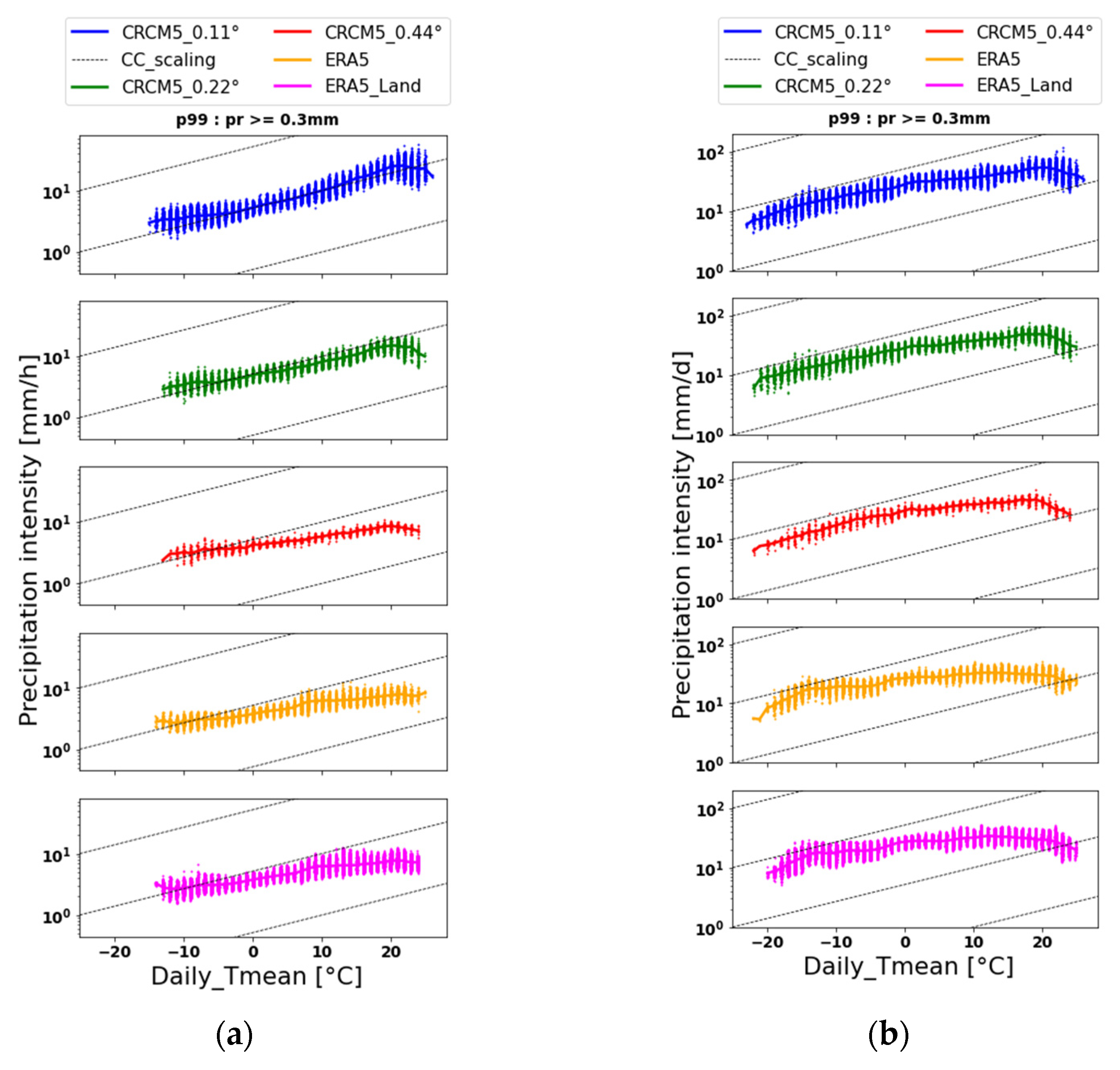
Figure 2. Evolution of the 99th percentile of: (a) hourly and (b) daily precipitation vs. the daily mean temperature for the domain #2 (ORB): CRCM5_0.11° (blue), CRCM5_0.22° (green), CRCM5_0.44° (red), ERA5 (orange), and ERA5_Land (magenta). The solid line indicates the mean value, and the dotted lines correspond to the scaling factor α = 6.8%/°C. Threshold to define wet days uses P ≥ 0.3 mm (where P is precipitation accumulated over 1 h or 1 day). All data series are from the 1981–2010 period.
Atmosphere 14 01130 g002
Figure 3. Scaling factor α calculated for all grid points of domain #2 using the least squares method to provide a linear relationship between hourly and daily extreme precipitation and Tmean. The correlation coefficient between the two variables is statistically significant at the 5% level (p-value ≤ 0.05). As in Figure 2, the threshold, P ≥ 0.3 mm, is used.
Atmosphere 14 01130 g003
Figure 4. Frequency distribution of the maximum values of the 99th percentile of (a) hourly and (b) daily precipitation ( P 99 _ max) for each grid point of domain #2, in joint occurrence with the average temperature at which this maximum value was reached. As in Figure 2, the threshold, P ≥ 0.3 mm, is used.
Atmosphere 14 01130 g004
Figure 5. Spatial distribution of the scaling factor α in the domain #1 for (a) hourly and (b) daily precipitation calculated from CRCM5_0.11°, CRCM5_0.22°, CRCM5_0.44°, ERA5, and ERA5_Land. As in Figure 2, the threshold P ≥ 0.3 mm is used.
Atmosphere 14 01130 g005
Figure 6. Seasonal variability of the scaling factor α in (a) winter and (b) summer for both hourly and daily precipitation (left and right panels for each season, respectively). As in Figure 2, the threshold P ≥ 0.3 mm is used.
Atmosphere 14 01130 g006
Figure 7. Same as Figure 3, but for (a) winter and (b) summer. The threshold P ≥ 0.3 mm is used.
Atmosphere 14 01130 g007
Figure 8. Same as Figure 4, but for (a) hourly and (b) daily precipitation (left and right panels, respectively) in winter (top panels) and summer (bottom panels). The threshold P ≥ 0.3 mm is used.
Atmosphere 14 01130 g008
Figure 9. Mean anomalies of GZ-500 (in color (m)) and of the MSLP (black contour lines (Pa)) for Situation A (days with Tmean < 15 °C in domain #3) for the months of (a) June, (b) July, and (c) August. Domain #3 is indicated in the maps by the small yellow box. All anomalies are computed with respect to the 1981–2010 climatological values of MSLP and GZ-500.
Atmosphere 14 01130 g009
Figure 10. Mean anomalies of GZ-500 (in color (m)) and of the MSLP (black contour lines (Pa)) for Situation B (days with 15 °C ≤ Tmean ≤ 25 °C in domain #3) for the months of (a) June, (b) July, and (c) August. Domain #3 is indicated in the maps by the small yellow box. All anomalies are computed with respect to the 1981–2010 climatological values of MSLP and GZ-500.
Atmosphere 14 01130 g010aAtmosphere 14 01130 g010b
Figure 11. Mean anomalies of GZ-500 (in color (m)) and of the MSLP (black contour lines (Pa)) for Situation C (days with Tmean > 25 °C in domain #3) for the months of (a) June, (b) July, and (c) August. Domain #3 is indicated in the maps by the small yellow box. All anomalies are computed with respect to the 1981–2010 climatological values of MSLP and GZ-500.
Atmosphere 14 01130 g011aAtmosphere 14 01130 g011b
Figure 12. Same as Figure 2, but for the CRCM6/GEM5 simulation during the period 2015–2021 for (a) hourly and (b) daily precipitation.
Atmosphere 14 01130 g012
Figure 13. Same as Figure 3a and Figure 4b (respectively), but for the CRCM6/GEM5 simulation during the period 2015–2021 for hourly and daily precipitation. Panel (a) corresponds to box plots of scaling factors for both hourly and daily precipitation (99th percentile values) for all grid points of domain #2 (Figure 1), and panel (b) is the mapping of the scaling factors over the ORB area.
Atmosphere 14 01130 g013
Figure 14. Same as Figure 6, but for the CRCM6/GEM5 simulation during the period 2015–2021 for (a) hourly and (b) daily precipitation during winter and summer seasons (top and bottom panels, respectively).
Atmosphere 14 01130 g014
Table 1. Description of the data used in our study: CRCM5, ERA5, ERA5-Land over the period 1981–2010, and CRCM6 over the period 01 September 2014 and 30 June –2022.
Model or ReanalysisPeriod CoveredResolutionVariablesLevels and Temporal ResolutionTime AverageUnits
CRCM501/01/1981–31/12/20100.44° (~50 km) 0.22° (~25 km) 0.11° (~12.5 km)Temperature
Total precipitation
2 m (3 h)
Surface (1 h)
Daily
1 hmax * and Daily
°C
mm/h
mm/d
CRCM601/09/2014–30/06/20220.0225° (~2.5 km)Temperature
Total precipitation
2 m (1 h)
Surface (1 h)
Daily
1 hmax * and Daily
°C
mm/h
mm/d
ERA501/01/1981–31/12/20100.25° (~31 km)Temperature
Total precipitation
2 m (1 h)
Surface (1 h)
Daily
1 hmax * and Daily
°C
mm/h
mm/d
Geopotential height500 hPa (1 h)Dailym2 s−2
Mean sea level pressureSurface (1 h)DailyhPa
ERA5-Land01/01/1981–31/12/20100.1° (~9 km)Temperature
Total precipitation
2 m (1 h)
Surface (1 h)
Daily
1 hmax * and Daily
°C
mm/h
mm/d
* Maximum hourly precipitation during a 24 h period.
Disclaimer/Publisher’s Note: The statements, opinions and data contained in all publications are solely those of the individual author(s) and contributor(s) and not of MDPI and/or the editor(s). MDPI and/or the editor(s) disclaim responsibility for any injury to people or property resulting from any ideas, methods, instructions or products referred to in the content.