Implementing and Improving CBMZ-MAM3 Chemistry and Aerosol Modules in the Regional Climate Model WRF-CAM5: An Evaluation over the Western US and Eastern North Pacific

Abstract

The representation of aerosols in climate–chemistry models is important for air quality and climate change research, but it can require significant computational resources. The objective of this study was to improve the representation of aerosols in climate–chemistry models, specifically in the carbon bond mechanism, version Z (CBMZ), and modal aerosol modules with three lognormal modes (MAM3) in the WRF-CAM5 model. The study aimed to enhance the model’s chemistry capabilities by incorporating biomass burning emissions, establishing a conversion mechanism between volatile organic compounds (VOCs) and secondary organic carbons (SOCs), and evaluating its performance against observational benchmarks. The results of the study demonstrated the effectiveness of the enhanced chemistry capabilities in the WRF-CAM5 model. Six simulations were conducted over the western U.S. and northeastern Pacific region, comparing the model’s performance with observational benchmarks such as reanalysis, ground-based, and satellite data. The findings revealed a significant reduction in root-mean-square errors (RMSE) for surface concentrations of black carbon (BC) and organic carbon (OC). Specifically, the model exhibited a 31% reduction in RMSE for BC concentrations and a 58% reduction in RMSE for OC concentrations. These outcomes underscored the importance of accurate aerosol representation in climate–chemistry models and emphasized the potential for improving simulation accuracy and reducing errors through the incorporation of enhanced chemistry modules in such models.

1. Introduction

Modeling atmospheric chemistry is central to global issues such as air quality and climate change, which have direct consequences on human livelihoods. Proper numerical representation of atmospheric chemistry calls for accurate simulations and coupling of meteorological and chemical processes [1]. The weather research and forecasting (WRF) model [2] coupled with chemistry (WRF-Chem) [3] has wide-ranging applications and demonstrable reliability in both research and forecasting areas of atmospheric chemistry. The application of WRF-Chem includes, but is not limited to, air quality predictions [4], future climate–chemistry projections [5,6], meteorology–pollution interactions [7], aerosol–cloud interactions [8,9], atmospheric energy budget investigations [10], and the characterization of biomass burning [11].

Atmospheric chemistry simulations carried out using WRF-Chem are sensitive to the selection of the chemistry parameterization schemes. In WRF-Chem, the chemistry parameterization schemes consist of multiple modules with different treatments for the gas, aerosol, and aqueous phases [3,12]. For each phase, the treatment and processing are represented by individual modules. Depending on the desired complexity, one may choose a chemistry suite of modules to cover all or some of the three phases [13]. For example, a bulk aerosol-only module, Goddard ozone chemistry aerosol radiation and transport (GOCART) [14], has been implemented into WRF-Chem without gas-phase ozone chemistry (chem_opt = 300), including only 18 chemical species. In contrast, a suite consisting of the model for ozone and related tracers (MOZART) [15] for gases and the model for simulating aerosol interactions and chemistry (MOSAIC) [16] for aerosols with eight sectional bins (chem_opt = 202) simulates interactions among all three phases. As one of the most complicated chemistry configurations in the current WRF-Chem model, MOSAIC could track as many as 143 gas species and all major aerosols, including sulfate, nitrate, ammonium, black carbon (BC), organic carbon (OC), mineral dust, and sea spray aerosols, with more than 300 reactions [15].

There is a tradeoff between model comprehensiveness and computational efficiency [17]. More complex chemistry parameterization schemes that consider additional species and reactions provide realistic representations of atmospheric chemistry [18]. However, these comprehensive modules are less practical for large-scale or long-term simulations due to their high computational demands, limiting their ability to characterize chemistry at detailed levels [19]. High spatial resolution in regional models to capture fine-scale features such as convective storms and interactions with fire-emitted aerosols increases computational costs and imposes constraints on the complexity of the chemistry modules used [20]. For instance, doubling the horizontal resolution in climate–chemistry models may result in an eightfold increase in computational requirements [21].

Efforts have been made to develop simplified representations of aerosol and chemistry processes for global and regional models while maintaining high accuracy. One example is the modal aerosol module (MAM) [22], initially developed for the community atmosphere model, version 5 (CAM5), which is part of the widely utilized community earth system model, version 1. MAM effectively handles major aerosol species such as BC, OC, sulfate, sea salt, and dust with reasonable accuracy. The use of modal or bulk aerosol approaches in regional climate models such as WRF dates to as early as 2004 [23].

A version of the MAM scheme, known as MAM3, combined with the CAM5 physics suite, was implemented in WRF-Chem by Ma et al. [24]. This version, referred to as WRF-CAM5, demonstrated consistently low biases in simulations of chemical species and aerosol optical depths (AODs) compared to observations in East Asia [25,26]. Notably, during the 2008 boreal spring DC-8 flight campaign in Alaska for Arctic research of the composition of the troposphere from aircraft and satellites, the simulated surface BC concentrations in WRF-CAM5 were up to three orders of magnitude lower than the observations, which Ma et al. [24] attributed to the coarse horizontal grid of the model. Increasing the model resolution to 10 km improved the agreement with observations but still resulted in mean concentrations two orders of magnitude lower. Nevertheless, previous studies have shown that WRF-CAM5 is a computationally efficient framework for high-resolution regional aerosol and climate simulations. Since it shares the same aerosol chemistry and atmospheric physics packages as global climate models such as CESM, WRF-CAM5 can also be utilized to investigate the impact of resolution on aerosol simulations and aerosol–cloud interactions, accounting for unresolved processes in global models [24].

This study aims to evaluate and improve the simulation of aerosols and chemistry in WRF-CAM5. Specifically, we focus on the western United States and the adjacent northeastern Pacific Ocean, motivated by the need to study the off-coast aerosols originating from both anthropogenic emissions and biomass burning which play an essential role in the interactions with marine stratus and stratocumulus clouds [27]. The WRF-CAM5 version used in this study, as an option in the released NCAR WRF-Chem 3.9.1.1, includes the gas-phase chemistry module choice of CBMZ along with other aerosol-phase chemistry module choices of MAM3 (see

Table 1. Physical and chemical schemes used in the WRF-CAM5 (with CBMZ-MAM3) simulations and the WRF-Chem (with MOZART-MOSAIC) simulations.

Physical or Chemical Scheme	WRF-CAM5 with CBMZ-MAM3	WRF-Chem with MOZART-MOSAIC
Gas-phase chemistry	CBMZ	MOZART
Aerosol	MAM3	MOSAIC (4-bins)
Photolysis	Fast-J	Madronich F-TUV
Emissions Read-in Scheme	RADM2 gas emissions to CBMZ with MAM3 aerosols	MOZART + aerosol emissions
Microphysics	CAM5: Morrison and Gettleman (Morrison et al., 2008 [28])	Morrison double-moment (Morrison et al., 2009 [29])
Cumulus	CAM5: Zhang–McFarlane	Grell–Freitas
Planetary Boundary Layer	CAM5: University of Washington	Yonsei University

). The only differences between WRF-CAM5 and other WRF-Chem setups are the choice of chemistry suites (CBMZ/MAM3, setting “chem_opt = 503” in the WRF-Chem) and the accompanying chemical and physical schemes. For detailed chemical and physical schemes, readers are referred to Section 2 and Table 1.

Similar to Ma et al. [24], the initial test runs using the default WRF-CAM5 indicate abnormally low aerosol concentrations and unrealistic spatial distributions, particularly over regions influenced by biomass burning. Here, we aim to improve the CBMZ-MAM3 chemistry modules in the WRF-CAM5 model to address two deficiencies identified:

(1)

The biomass burning emissions are completely ignored for both aerosol-phase (MAM3) and gas-phase (CBMZ) chemistry;

(2)

The mechanism that converts VOC to SOC is not included.

While the default WRF-CAM5 does not include the VOC-to-SOC pathway, more than 50% of the total aerosols in urban areas may be SOCs [30], and previous observations for total aerosol composition have indicated a dominant role of secondary sources for total organic carbon [31]. SOCs are formed by the oxidation of VOCs [32]. This poses an inherent challenge for numerical modeling because there are many different types of VOCs (>10³).

In this study, the model improvement incorporated for treating the SOC formation follows the implementation of MAM3 for secondary organic aerosol in the global model CAM5 [22]. The implementation of MAM3 in the WRF framework will allow us to evaluate the same aerosol schemes used by CAM but at finer spatial resolutions that are comparable to the observational dataset, making it feasible to transfer lessons learned about aerosol simulations and interactions with clouds from the high-resolution regional studies to the coarser-resolution global models. The improved WRF-CAM5 with MAM3 would thus provide a useful tool for assessing the global model parameterizations, in addition to the benefit in computational efficiency from the more sophisticated WRF-Chem schemes.

We describe the detailed model setup in Section 2 and our modifications in Section 3. In Section 4, we validate the original and enhanced simulations. The simulations are presented in a step-by-step manner to shed light on the relative importance of various progressive implementations of the proposed approach. The simulated aerosol distributions off the western coast of the US will be analyzed to demonstrate the performance of the updated models. We then conclude this study in Section 5.

2. Methods

2.1. Model

We used version 3.9.1.1 of the WRF model [33] coupled with chemistry [3], and CAM5 for the physics mechanism as the base model of WRF-CAM5 in this study. Longwave and shortwave radiation processes are parameterized by the rapid radiative transfer model (RRTM) developed for general circulation models (RRTMG) [34]. The land-surface processes were simulated by the unified Noah model [35].

The main objective of this study is to improve the coupled CBMZ-MAM3 chemistry scheme [22,36] in WRF-CAM5 as a workable configuration for simulating aerosols and chemistry over the western US and the adjacent northeastern Pacific. MAM3 is implemented similarly to as in global modeling studies [22]; it simulates major aerosol species such as BC, OC, dust, sulfate, and sea salt, but does not include nitrate chemistry. Additionally, MAM3 distinguishes between hydrophilic and hydrophobic species and there is an aging process that transforms hydrophobic BC/POC to hydrophilic BC/POC [22], and the time for such a process is prescribed to be 1–2 days. In WRF-CAM5, MAM3 has been linked to CBMZ gas-phase chemistry, a carbon-bond mechanism that includes 73 chemical species and 237 reactions (chemistry option 503) [23].

We also consider MOZART-MOSAIC [15,16], the most comprehensive and expensive chemistry scheme in WRF-Chem, as a benchmark for comparison with CBMZ-MAM3. MOSAIC simulates most major aerosol species, such as BC, sulfate, ammonium, OC (both primary and secondary), nitrate, and chlorides (Cl), with either four or eight size bins. This study uses the four-bin version of the MOZART-MOSAIC suite, which involves 143 gas-phase species with 347 reactions. In contrast, CBMZ-MAM3 uses the bulk mechanism and approaches the detailed chemical species with the lumped-group mechanism for most of the gas-phase chemistry [22]. Therefore, one would expect a more realistic simulation with MOZART-MOSAIC, given its more comprehensive representation of chemical processes. This notion will be tested in our simulations.

Ideally, we want to use the same physical schemes for the two simulations to isolate the chemistry impact, but this will result in chemistry–physics compatibility issues that either cause model errors or yield unrealistic simulations. The detailed model configurations are shown in Table 1, which summarizes the key differences between the two configurations. For the CBMZ-MAM3 simulation, the planetary boundary layer (PBL) processes are parameterized using the University of Washington shallow convection and moist turbulence schemes [37] as in CAM5. For the MOZART-MOSAIC simulation, we chose the Yonsei University PBL [38]. For the cloud microphysics scheme, the CBMZ-MAM3 simulation uses the CAM5 Morrison–Gettelman scheme [29], and the MOZART-MOSAIC simulation adopts the Morrison two-moment scheme [28]. Furthermore, the photolysis scheme for the CBMZ-MAM3 suite is coupled with Fast-J photolysis [39], and the photolysis option for the MOZART-MOSAIC simulation is fast troposphere ultraviolet–visible [40].

2.2. Simulations

The simulation domain spans from 180° to 93° W and 9° to 55° N (Figure 1) with 27 vertical layers up to 100 hPa. The horizontal grid spacing is uniformly set to 36 km × 36 km. A series of 1-month simulations (from 1 June to 30 June 2013) is used for the model assessment, which overlaps with the duration of the marine atmospheric radiation measurement (ARM) global energy and water cycle experiment (GEWEX)–cloud system study (GCSS)–Pacific cross-section intercomparison investigation of clouds campaign (MAGIC; see Section 2.3.4).

The meteorological initial and boundary conditions were obtained from the 6-hourly National Centers for Environmental Prediction final analysis (NCEP-FNL). The simulated meteorological conditions were nudged to NCEP-FNL every 6 h; the chemical initial and boundary conditions were obtained from the global simulations of the community atmosphere model with chemistry, version 5 [41]. The nudging domain is the entire model domain shown in Figure 1. Vertically, the nudging is performed for model layers above the PBL. The meteorological variables nudged are winds, temperature, and the mixing ratio of water vapor.

For anthropogenic emissions from the continental United States, we used the U.S. Environmental Protection Agency (EPA) national emissions inventory (NEI) [42]. For the rest of the model domain outside the continental United States, we used version 2 of the emission database for global atmospheric research, developed as a part of hemispheric transport of air pollution (EDGAR-HTAP v2) [43]. EPA-NEI has a spatial resolution of 12 km × 12 km, and EDGAR-HTAP has a spatial resolution of 0.1° × 0.1°. Both datasets were re-gridded to the model resolution over the simulation domain using a mass-conserving emissions pre-processor. For the dust scheme, we use dust emissions coupled with MOSAIC and the modal aerosol dynamics model for Europe/secondary organic aerosol model (MADE/SORGAM).

The latest EPA-NEI inventory available is for 2014 (a 1-year difference from our simulation year), and the latest EDGAR-HTAP emissions were for 2010 (a 3-year difference). EPA emissions have diurnal cycles and are distinguished by weekdays and weekends, assuming that weekday emissions are stronger in urban areas than on weekends (EPA, 2018). Therefore, we adjusted the calendar and ensured that the adopted emissions follow the 2013 weekday and weekend patterns. We mapped the EPA-NEI emissions to the model grids by using the sparse matrix operator kernel (SMOKE) modeling system to yield hourly emission input data. The EDGAR-HTAP emissions include diurnal cycles only (as an hourly dataset) without any weekday–weekend contrast and do not require any adjustments.

For biomass burning emissions, we used the emissions from the fire inventory from NCAR (FINN) [44], a widely used satellite-based fire-related emissions inventory with a horizontal resolution of 1 km × 1 km with hourly updates. FINN has speciated emissions including BC, OC, CO, VOCs, etc. For biogenic emissions, we used the model of emissions of gases and aerosols from nature (MEGAN) [45], which calculates biogenic emissions online within the model at every time-step using the model-simulated environmental conditions.

In addition to using the default level of emissions in the published datasets, we also performed a sensitivity simulation by increasing both anthropogenic and biomass burning aerosol and VOC emissions by a factor of 3.

2.3. Observations

We assessed the model performance by comparing the model simulations against ground-based observations, shipboard measurements, satellite retrievals, and reanalysis products. The detailed data sources and variables used for model assessment are shown in

Table 2. Sources of observations for evaluation.

Data Source	Data Source Links	Variables Provided
Aerosol robotic network (AERONET)	https://aeronet.gsfc.nasa.gov/ accessed on 20 June 2023	AOD
Interagency monitoring of protected visual environments (IMPROVE)	http://vista.cira.colostate.edu/Improve/ accessed on 20 June 2023	surface concentrations of BC and OC
Environmental Protection Agency (EPA)	https://www.epa.gov/aqs accessed on 20 June 2023	surface temperatures; surface concentrations of CO
The modern-era retrospective analysis for research and applications, version 2 (MERRA-2)	https://gmao.gsfc.nasa.gov/reanalysis/MERRA-2/ accessed on 20 June 2023	surface temperatures; surface concentrations of BC, CO, and OC; AOD
Tropical rainfall measuring mission (TRMM)	https://gpm.nasa.gov/data/directory accessed on 20 June 2023	precipitation
Cloud–aerosol lidar and infrared pathfinder satellite observations (CALIPSO) based on SODA algorithm	https://www-calipso.larc.nasa.gov/ accessed on 20 June 2023	AOD
MAGIC ship campaign for June 2013	https://www.arm.gov/research/campaigns/amf2012magic accessed on 20 June 2023	surface temperatures; AOD

.

2.3.1. MERRA-2 Reanalysis Product

We used modern-era retrospective analysis for research and applications, version 2 (MERRA-2) [46] to validate the simulated meteorology, surface concentrations of chemical species, and column aerosol optical depth (AOD). MERRA-2 assimilates the AOD from both satellite platforms (e.g., MODIS, AVHRR, and MISR) and ground-based measurements (AERONET) [47]. Studies have found generally acceptable AOD agreements among MERRA-2, satellite products, and ground-based measurements [22,48,49]. Although, as an observationally constrained reanalysis product, MERRA-2 should not be considered the ground truth, it has been tested for authenticity in our study domain [47,50]. Because reanalysis products are spatially complete, they enable us to conduct model evaluations for large-scale spatial patterns.

2.3.2. Ground Observations from the EPA, Aerosol Robotic Network, and Interagency Monitoring of Protected Visual Environments

In addition to the reanalysis products, we also validated the meteorology and chemistry against ground-based observations representative of urban, remote, and biomass-burning-influenced areas.

For both the surface temperature and CO mixing ratios, we used the EPA air quality system (AQS) for evaluation [51]; the AQS has been extensively applied for both meteorological and chemical evaluations in our study domain [52,53]. We selected six urban sites within the domain for model evaluation: Irvine, California; San Diego, California; Salt Lake City, Utah; Denver, Colorado; Seattle, Washington; and Phoenix, Arizona.

The simulated AOD results are also compared to the aerosol robotic network (AERONET) [54] from the National Aeronautics and Space Administration (NASA). AERONET is a ground-based remote-sensing aerosol network that uses sun- and sky-scanning radiometers to measure aerosol optical properties [55]. In a manner similar to the EPA AQS sites, we selected six AERONET sites within the simulation domain for model evaluation, including CalTech (Pasadena), California; Santa Monica, California; Kelowna, British Columbia; White Sands, New Mexico; Hermosillo, Mexico; and Neon-Civalla, Colorado.

The simulated surface BC and OC concentrations were compared to the interagency monitoring of protected visual environments (IMPROVE) network. The IMPROVE network primarily measures the BC and OC at national parks and national monuments [56], and samplers collect 24 h samples every 3 days [57]. We selected six IMPROVE network sites for model evaluation, including Phoenix, Arizona; Fresno, California; Puget Sound, Washington; Lava Beds, California; Great Basin, Nevada; and San Rafael, California. The selection of the AERONET and IMPROVE sites provided the required spatial distancing to check the model’s performance in different regions.

2.3.3. Satellite Observations

Apart from ground-based observations, we also included satellite products for further evaluation because of their broad spatial coverage.

For precipitation, we used daily observations of total precipitation from the tropical rainfall monitoring mission (TRMM) [58]. The validity of the TRMM products has been extensively examined in North America with relatively reliable results [59]. Note that WRF-CAM5 saves precipitation output in a cumulative manner (i.e., in the total amount for a month). We calculated the precipitation from both the TRMM products and simulation output as hourly values (i.e., millimeters per hour) for direct comparison.

For AOD over the northeastern Pacific Ocean, we use synergized optical depth of aerosols (SODA) [60,61,62] retrievals. SODA AOD is a product derived from cloud–aerosol lidar and infrared pathfinder satellite observations (CALIPSO) surface return that has been proven to show excellent agreement with other airborne and satellite datasets [60,62]. SODA AOD does not depend on an a priori aerosol classification scheme, unlike the standard CALIPSO product; therefore, the retrievals are unaffected by biases attributed to layer under-detection and aerosol type misclassification. Because SODA is derived from CALIPSO-attenuated backscatter, the SODA spatial resolution is identical to CALIPSO (333 m). CALIPSO has a relatively narrow cross-track beam width (~70 m at the Earth’s surface) [63] because the beam is fixed at a near-nadir viewing direction [64] and, therefore, the retrievals cover a fraction of a WRF-CAM5 grid cell. Here, we sampled the WRF-CAM5 model grid cells closest to the CALIPSO center line for each observational time-step and took the average on a daily basis.

For CO evaluation, we used measurements of pollution in the troposphere (MOPITT) [65] for surface CO mixing ratios. MOPITT adopts correlation spectroscopy to derive the column-integrated CO levels. The derivation of surface CO mixing ratios is implemented by Worden et al. [66].

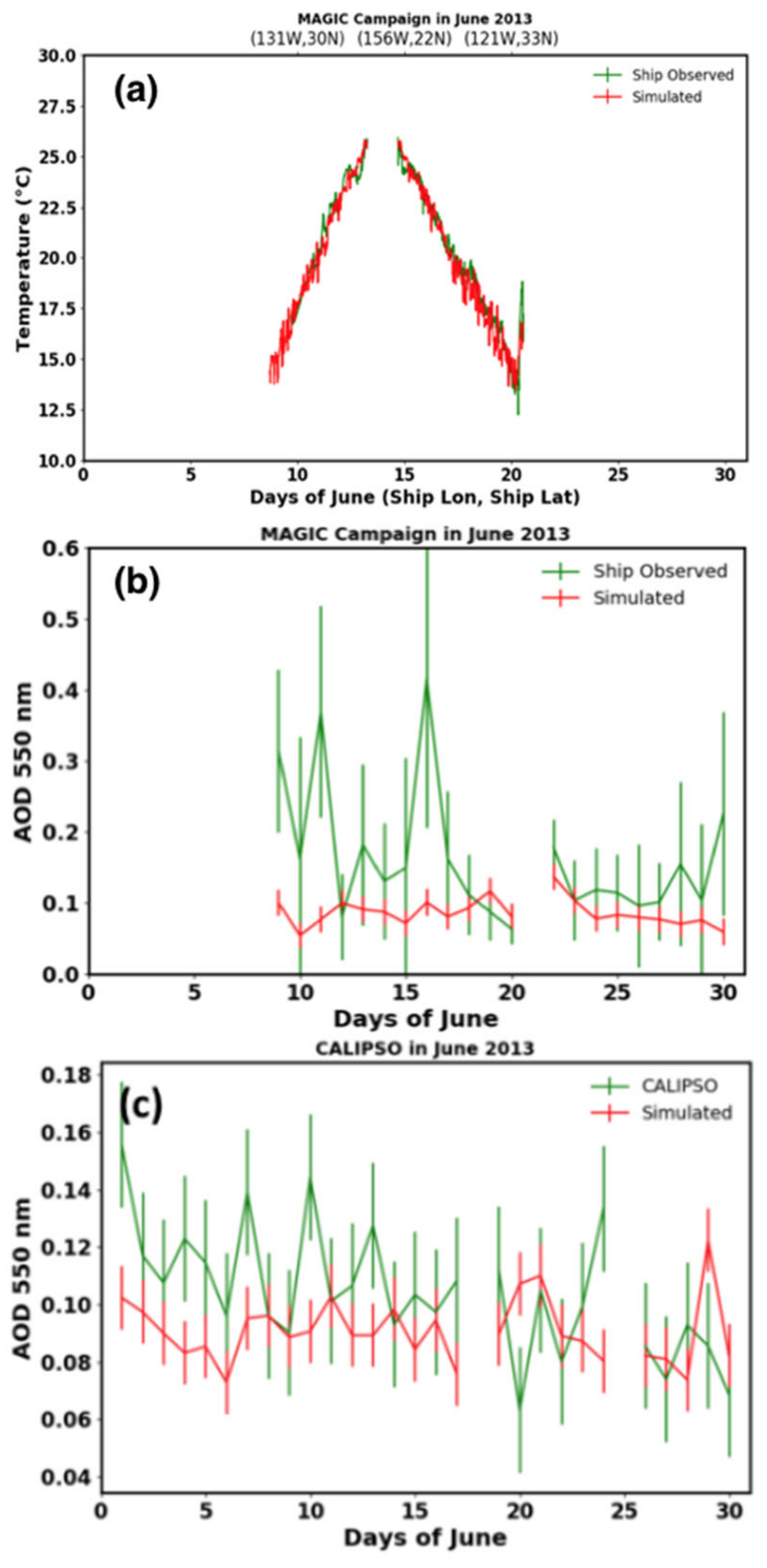
2.3.4. MAGIC Ship Campaign

In June 2013, a C-9 class ship, serving as part of the marine atmospheric radiation measurement (ARM) global energy and water cycle experiment (GEWEX)–cloud system study (GCSS)–Pacific cross-section intercomparison investigation of clouds (MAGIC) [27] missions traveled round-trip between Los Angeles, California, and Honolulu, Hawaii. This MAGIC field campaign [27,67] provides valuable in situ data for the model evaluations over the ocean.

The focus of MAGIC is on marine clouds with measurements such as temperature, winds, carbon monoxide, AOD, and cloud condensation nuclei. There are no other detailed aerosol chemical measurements. In June 2013, a campaign vessel made a round-trip voyage between Los Angeles, California, and Honolulu, Hawaii (Figure 1a). In this study, we used the surface temperature and AOD from the MAGIC campaign [27] to evaluate our simulations over the northeastern Pacific. The temperature data from the MAGIC campaign were collected every minute, while the AOD data were collected intermittently. To match the simulation, the surface temperature data were averaged to an hourly resolution, and the AOD data were averaged to a daily resolution.

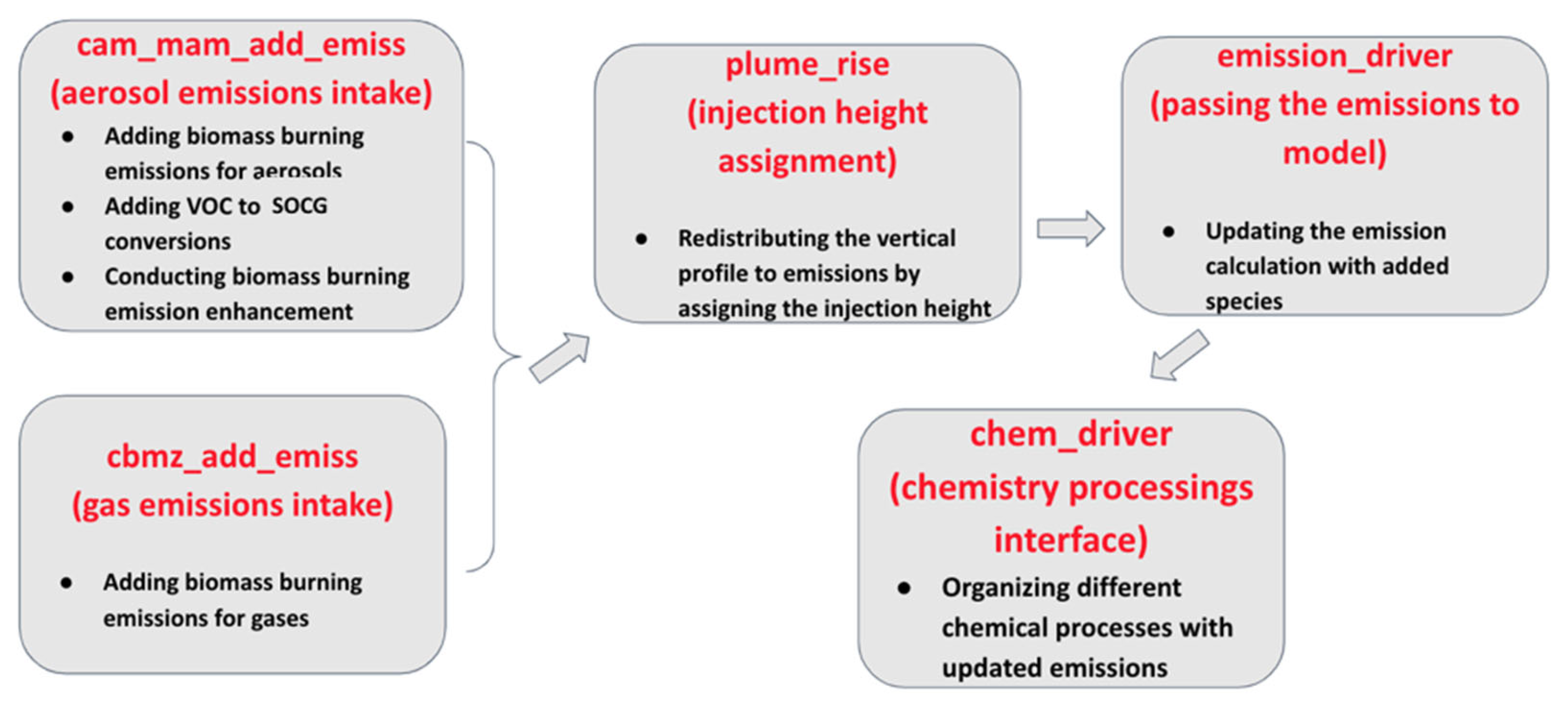
3. Model Improvements and Code Modification

We modified two major WRF-CAM5 modules, MAM3 and CBMZ, to mitigate two specific deficiencies: missing biomass burning emission processes in both MAM3 and CBMZ, and missing VOC-to-SOC conversion mechanisms. To illustrate these modifications, we performed six sets of simulations, four of which documented progressive improvements, one of which employed increased emissions, and the last of which was a benchmark run with the more sophisticated MOZART-MOSAIC chemistry suite. All simulations used the same chemical and meteorological initial and boundary conditions described in Section 2.2. Specifically, these simulations are summarized in

Table 3. Names and descriptions of each simulation case. Note that each of these configurations is an additional change based on the configuration in Table 1, except for configuration (f).

Configuration	Short Name	Description
a	Baseline	Baseline configuration (Ma et al., 2014 [24])
b	AddingBBaerosol	Aerosols from biomass burning emissions added to MAM3
c	AddingBBgas	Gases from biomass burning emissions added to CBMZ
d	AddingSOC	VOC-to-SOC conversions added
e	TriplingEmission	3× anthropogenic and biomass burning emissions
f	MOZART-MOSAIC	The MOZART-MOSAIC run (Wu et al., 2019 [7])

as follows:

(a)

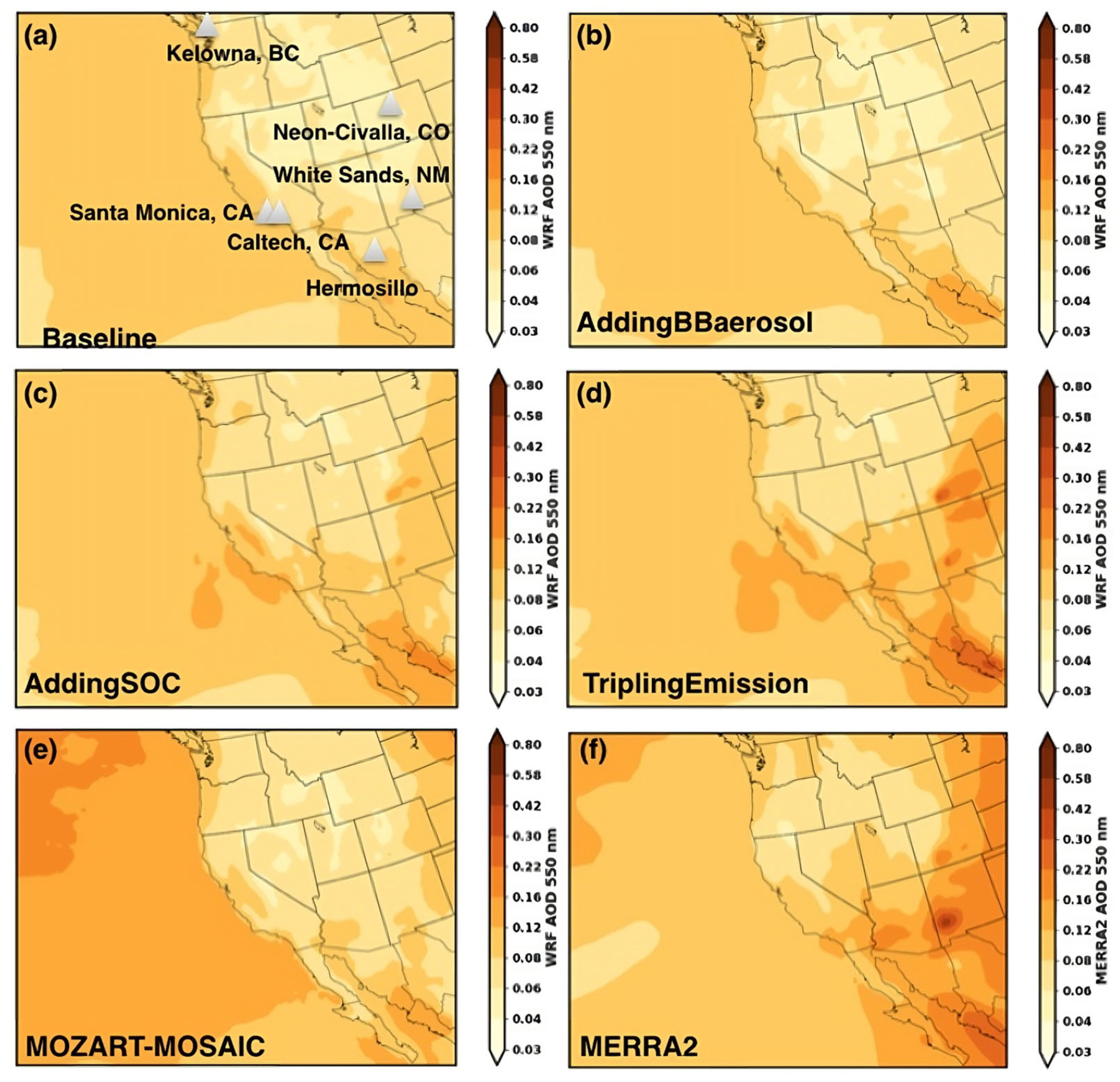
The baseline run with the original WRF-CAM5 coupled with CBMZ-MAM3 (baseline) in the NCAR-released WRF-Chem model. This is a similar setup as developed by Ma et al. [24].

(b)

A run including the capability of incorporating biomass burning aerosol emissions in MAM3 (AddingBBaerosol), such as BC and OC.

(c)

A run including configuration (b), as well as the capability of incorporating biomass burning emissions of gaseous species in CBMZ (AddingBBgas), such as CO and VOCs.

(d)

A run including configuration (c), as well as the conversion mechanism from VOCs to SOC through an intermediate product SOCG (SOC gas; see Section 3.2 for details) (AddingSOC);

(e)

A run including configuration (d) and increasing both anthropogenic and biomass burning emissions by three times the inventory levels (TriplingEmission);

(f)

A benchmark run with the MOZART-MOSAIC chemistry suite (MOZART-MOSAIC), which is similar to the setup of Wu et al., (2019) [7].

3.1. Accounting for Biomass Burning Emissions in CBMZ-MAM3

Adding the capability of incorporating biomass burning emissions into the CBMZ-MAM3 chemistry suite involves supplying the emitted species to these two modules separately. The first step is to add emitted aerosol-phase species to the MAM3 module. We added three major aerosols emitted by burning biomass—BC, primary OC (POC), and sulfate—to the MAM3 read-in module. By default, MAM3 partitions the aerosols into three modes: Aitken, accumulation, and coarse. In this modification, we added all species to the accumulation mode, where most of the biomass burning aerosol masses reside.

Next, we added gas-phase chemical species emitted by burning biomass to the CBMZ module. The following primarily emitted gas species were added: SO₂, NO₂, NO, NH₃, CO, CH₃COCHO, CH₃OH, C₂H₅OH, and C₅H₆O₂. Among the species listed, SO₂ has an oxidation mechanism to produce aerosol-phase products (e.g., sulfate); however, NO_x species (NO and NO₂) did not lead to nitrate production because MAM3, by default, does not integrate a nitrate chemistry mechanism [22].

3.2. Enabling VOC-to-SOC Conversion

Apart from neglecting the biomass burning emissions, another major issue with the current CBMZ-MAM3 module in WRF-CAM5 is the lack of accounting for SOCs (called SOAs in Liu et al. [22]; we use carbons instead of aerosols in the definition here and, therefore, refer to them as SOCs).

A more applicable approach is to group the VOCs either by molecule or structure [68], or by volatility [69,70]. However, both approaches can still be computationally demanding, depending on the number of groups simulated by the model and the complexity of the SOC-related chemistry the model needs. MAM3 adopts a simplified, less costly approach because it was built to provide a “minimal representation” of aerosol particles in global climate models.

MAM3 treats the formation of SOCs in a yield-based bulk mechanism from a predefined intermediate variable called SOCG (called SOAG in Liu et al. [22]; similar to SOC, we use carbons instead of aerosols in the definition here). SOCG is emitted as a single lumped semi-volatile organic carbon gas species and the SOCG emissions are calculated from primary VOCs (alkanes, toluene, isoprene, etc.) based on the fixed mass yields [22], as described in Equation (1):

$$\mathit{S}\mathit{O}\mathit{C}\mathit{G}={{\displaystyle \sum }}_{\mathit{i}\mathit{=}\mathbf{1}}^{\mathit{n}}{\mathit{C}}_{\mathit{V}\mathit{O}{\mathit{C}}_{\mathit{i}}}\ast \mathit{y}\mathit{i}\mathit{e}\mathit{l}{\mathit{d}}_{\mathit{i}},$$

(1)

where $C_{VO{C}_i}$ represents the concentration of individual VOC species (in parts per billion, ppb) that contributes to the total SOCG, and $yiel{d}_i$ represents the corresponding empirically determined yield factors. The typical range for the yield factors is 5–25% [22].

Here, we follow Liu et al. [22]: a total of six groups of VOC species are added to calculate the intermediate variable (SOCG) as an input to the MAM3 aerosol module. These added VOC species are big alkanes, big alkenes, isoprene, toluene, monoterpenes, and hydroxyacetone (also known as acetol). Among these six groups of species, the first five were defined by Liu et al. [22], while the last species (hydroxyacetone) was added to this study. Adding hydroxyacetone can improve the simulation results because it is the dominant species among all emitted VOCs in the FINN inventory. The contributions of hydroxyacetone toward SOC formation have been documented in several previous studies [71,72].

The yield factor of each species was assumed to be 15%, except for isoprene and monoterpenes, which were assumed to be 4% [73] and 25% [74], respectively. In the CAM-MAM3 implementation, SOCG is treated as an active tracer, once emitted, the aerosol module MAM3 then calculates condensation/evaporation of the SOCG to/from the aerosol modes, based on the thermodynamic equilibrium between the gas and aerosol phases. Liu et al. [22] showed that SOCG is predominantly removed by conversion to SOC. To reduce model complexity, we did not address the removal of SOCG.

Note that the yield factors for the big alkanes and alkenes we adopted are higher than the values (5%) used in Liu et al. [22] and lead to better model performance (see Section 4). The empirical basis for using a simple treatment for SOC formation is to assume that the mass yield from the precursor (VOCs) to SOC is at a fixed level. MAM3 further simplifies such a process by lumping all VOCs into one intermediate species called SOCG. Similar methods have been adopted by other chemistry–climate models (e.g., GEOS-Chem and CAM-Chem) [41,75,76], while more sophisticated approaches for representing SOA are also adopted in others [77,78].

3.3. Modifications to Enhance Emissions

We also conducted a sensitivity test for emission enhancements after we completed the two major modifications above. To increase the aerosol emissions, we applied a scaling factor of 3 to both the anthropogenic and biomass burning emissions in the MAM3 module by multiplying them by the incorporated emission fluxes from the inventories. Then, the updated emissions were passed to any subsequent modules.

Previous studies have suggested that both anthropogenic and biomass burning emissions are underestimated in the current inventories over the US. For anthropogenic emissions, Russo et al. [79] have found that the NEI underestimates the emissions from natural gas facilities, and [80] noticed that the NEI underestimates VOCs, a key component of SOA modifications performed in this study, from industrial sources. For biomass burning, we used FINN as the inventory, which relies on MODIS to detect fires. Thus, FINN is known to suffer from underestimation due to the following factors [44,81]: (a) MODIS cannot detect small and/or smoldering fires, and (b) MODIS cannot detect a fire region if it is covered by clouds.

We acknowledge that increasing the emissions by a factor of 3 is empirical, which is based on our preliminary tests to best match the domain-averaged AOD observations. However, it is needed sometimes in modeling studies (including WRF-Chem) to address the uncertainties in the emission inventories in order to resolve the discrepancies from the real-world observations [82,83,84].

3.4. Modifications to Other Related Modules

In addition to the two chemistry modules described above, we also modified other accompanying modules that use their output for further processing. Three additional modules serve these purposes (Figure 2): the chemistry-driver, emissions-driver, and plume rise modules. For the chemistry-driver and emissions-driver modules, the required modifications are to add newly incorporated variables from the biomass burning emissions, pass these variables to the two gas-phase chemistry and aerosol modules, and define and compute a new species variable for SOCG.

For the plume rise module [85], additional adjustments are necessary. The first step is to redistribute surface emissions into a number of vertical levels simulated by the model. In this case, FINN assumes that biomass burning emissions all originate from the surface, and the level is therefore set to 1. Then, we pass each emitted species to the vertical redistribution section where the plume rise module extracts the read-in emissions, distributes them vertically, and assigns injection heights for each species sourced from FINN. In the WRF-CAM5 used here (and the common plume rise module in the default WRF-Chem as well), the injection height is assigned by multiplying the original surface emissions by a weighting factor at each model level calculated online by the plume rise module. A vertical redistribution computed in this manner is considered near-real-time (occurring simultaneously with emission) [17]. Note that original WRF-Chem uses the Freitas et al. [85] plume rise scheme by including the sub-grid scale plume rise of vegetation fires in low-resolution atmospheric transport models. For detailed calculations of plume rise, please refer to Section 2 of Freitas et al. [85].

In addition to the module modifications described above, all the newly added species must be defined in the WRF-CAM5 registry file. We coupled the CBMZ-MAM3 module to WRF-CAM5 using the second-generation regional acid deposition model (RADM2) [86], and the emissions read-in option was defined as option 9 in WRF-CAM5. However, the current version of WRF-CAM5 (3.9.1.1) does not list exhaustive VOC species in the registry; thus, changing the chemistry modules alone without editing the registry would result in a significant underestimation of the total SOC because the model ignores the major VOC species we added. Therefore, we must add all the currently missing VOC species to the chemistry registry and align the species names in the model to be consistent with the emissions inventory. By doing so, we allow the MAM3 chemistry module to recognize the added VOC species and process them.

4. Results

In this section, we provide a comprehensive evaluation of the model performance based on the setup in Section 2 and improvements made in Section 3.

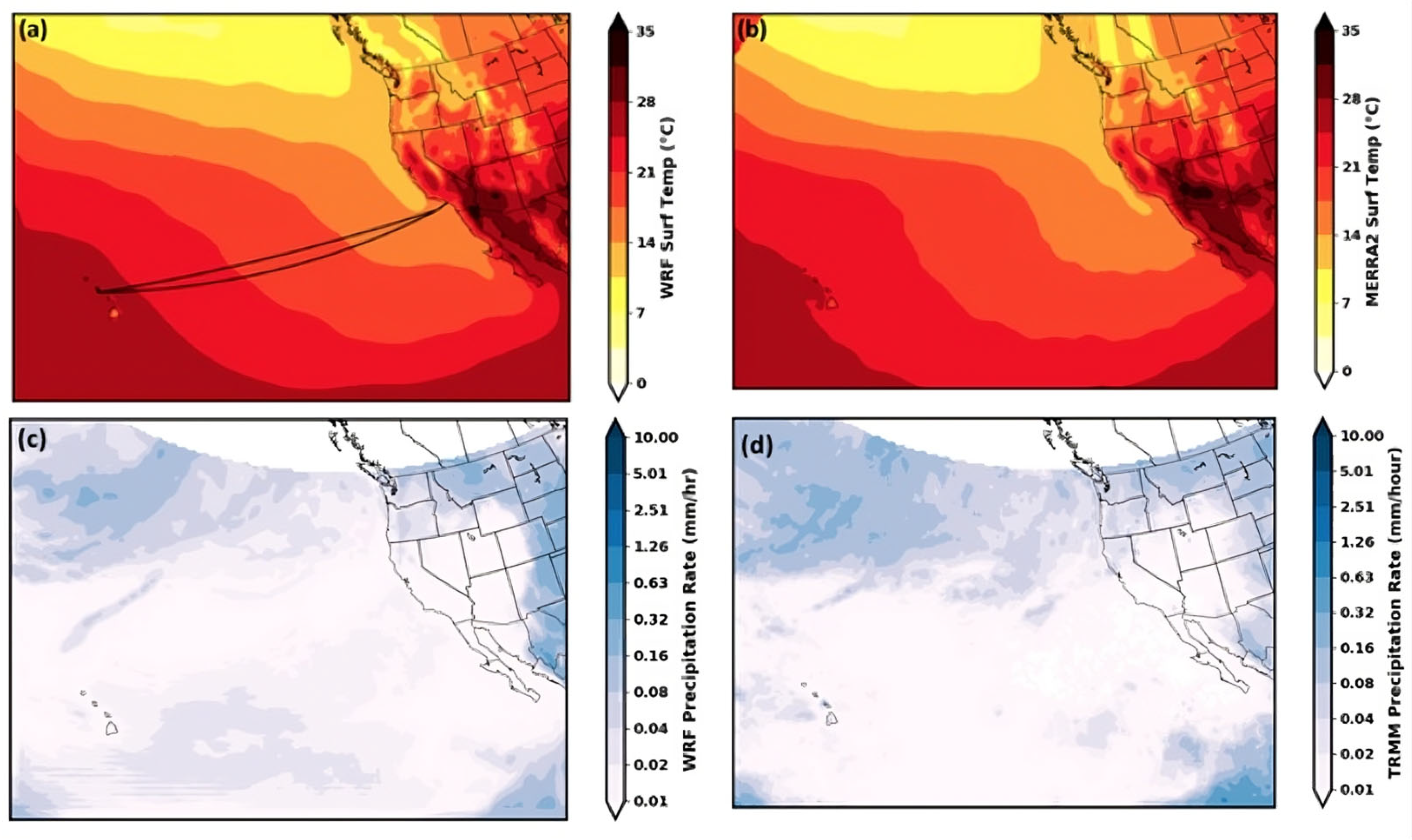
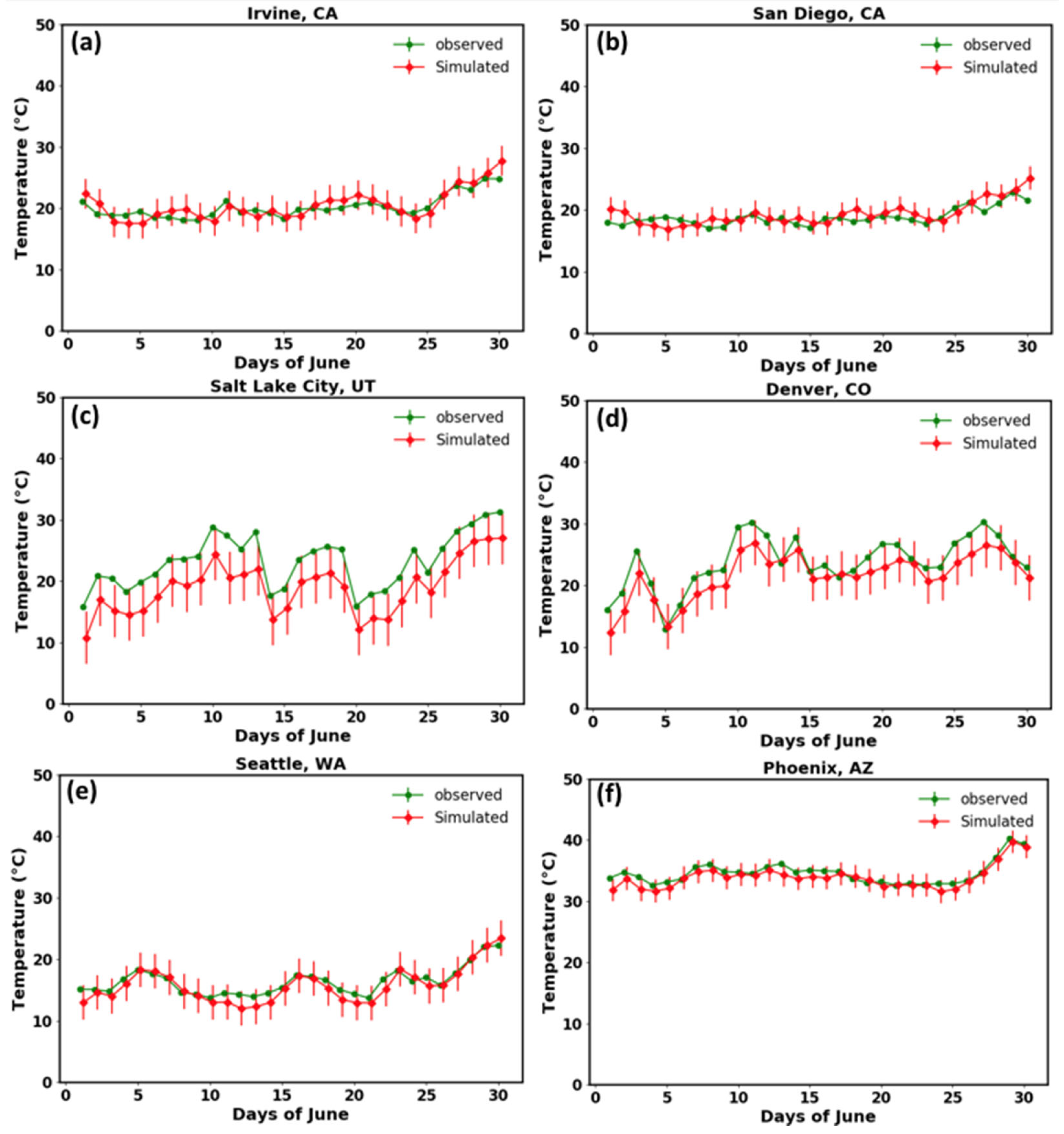
4.1. Meteorological Evaluation

First, we validated the simulated meteorology. Figure 1 shows the spatial distribution of the monthly surface temperature and precipitation from WRF-CAM5 in June 2013. Compared to the MERRA-2 and TRMM observations, the simulations nudged by the 6-hourly NCEP-FNL meteorology are consistent with the observations, with mean biases of 0.26 K and 0.01 mm/h. Please note that the color bars are in log scale and the difference within the same color code may not be negligible. Using log-scale color bars enables us to demonstrate that the simulated results and TRMM products are of a similar spatial pattern, in particular, for the regions where the precipitation rate is low. For the surface temperature, the WRF-CAM5 simulation successfully identifies the hot regions inland (near Arizona and Baja California). For precipitation, TRMM identifies the central Pacific and eastern tropical Pacific as regions with strong precipitation; both are captured by the WRF-CAM5 model. For inland areas, the simulation agrees with the TRMM data, which indicated that Colorado and New Mexico experienced more precipitation.

For the surface temperatures, we also evaluated the simulations against observations from six cities with consistently high temperatures (Figure 3). The simulated results have less than 2 K biases for all sites except Salt Lake City, Utah, and Denver, Colorado. For Salt Lake City and Denver, the simulated results have cold biases of less than 4 °C. Note that the cold biases in Denver and Salt Lake City are considered to be related to the topography. Because the simulation grid spacing is 36 km, it includes part of the surrounding areas for both cities; however, both Denver and Salt Lake City are surrounded by mountains and, therefore, grid boxes containing these cities have higher model elevation values than the real-world observational sites do. Therefore, a lower simulated temperature is expected. Nonetheless, for the period simulated, all days were within the range of anticipated uncertainties. Furthermore, we also evaluated the simulated temperature against the MAGIC campaign (Figure 4a); the simulated results are highly consistent with the ship observations. For each observational time-step (1 h), our simulated surface temperature is within 1 K of the ship observations.

Here we select the centerline of the CALIPSO-SODA retrieval that is the closest to the WRF-CAM5 simulation grid for each observational time-step and take the average on the daily basis. We have collected the CALIPSO-SODA AODs at finer spatial scales to the WRF grid. Since there is one daily satellite overpass, at 1:30 pm local time, the day-to-day variability in the model and observations is indicated by the error bars shown in Figure 4c.

4.2. Evaluation and Progressive Improvement of the Chemical Output Due to Model Enhancements

In this section, we validate the chemical species and demonstrate the step-by-step model improvements made.

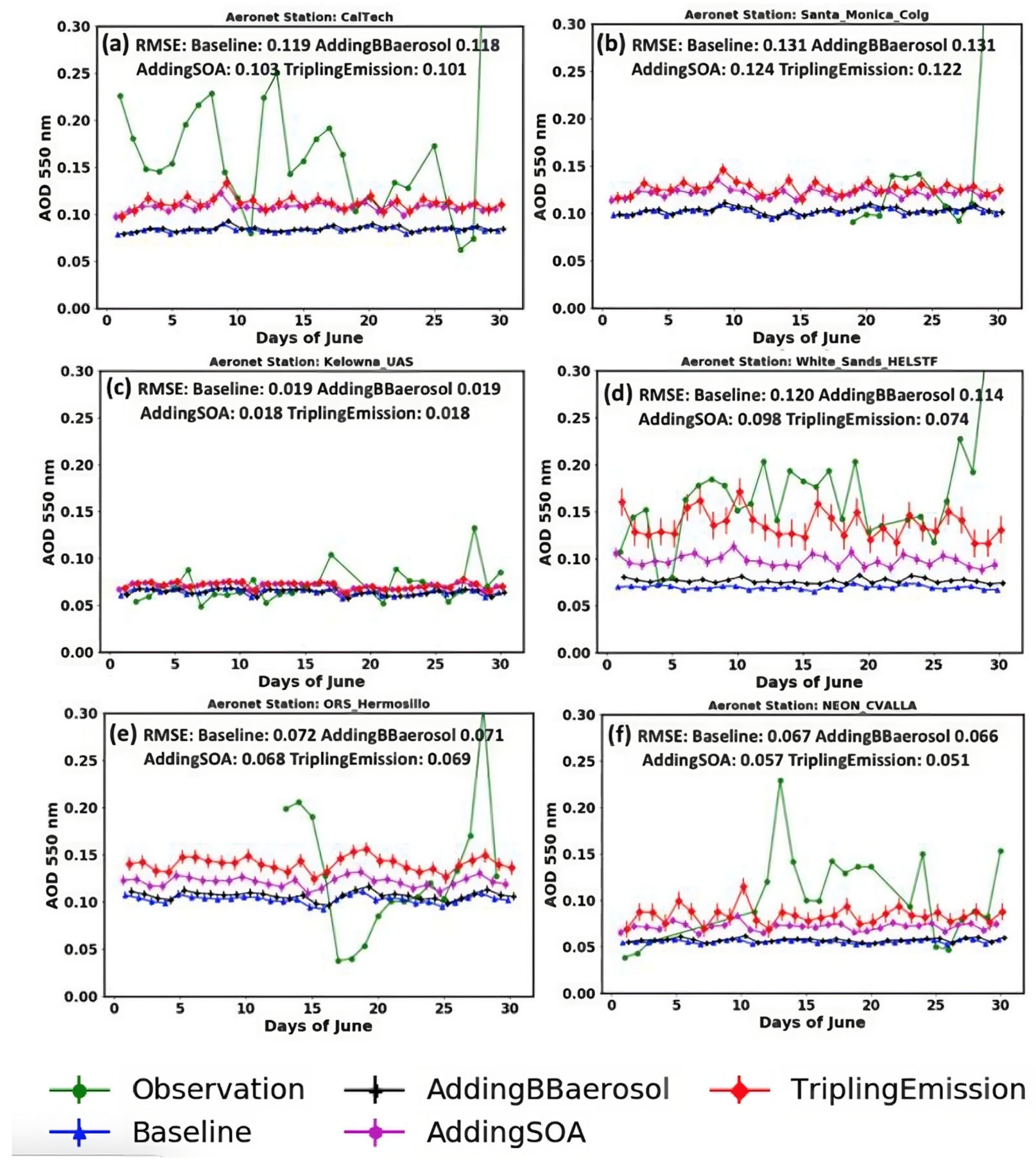
4.2.1. Improvements to the AOD

We first evaluated the simulated AOD at 550 nm against both the reanalysis products and station observations (Figure 5 and Figure 6). Generally, the point-based observations at individual stations have higher simulated AOD levels than their reanalysis product counterparts do. The AOD improvements after adding the biomass burning emissions of aerosols (AddingBBaerosol) were small (from 0.04 to 0.05) in the United States, and they cannot capture the hotspots seen in the MERRA-2 products on the monthly mean basis. The largest improvements in the model AOD are seen in parts of Mexico. After enabling the VOC-to-SOC conversions (AddingSOC), the spatial pattern in the United States becomes more consistent with that of MERRA-2; however, the magnitude is still much smaller (by a factor of ~2–3). Therefore, we further compared the MERRA-2 products with a tripled emission run (TriplingEmission) and found a much smaller model bias—about 0.05—under this configuration for the regions in both the United States and Mexico. Almost all the hotspots shown in MERRA-2 are captured by the model simulation of monthly AOD; however, the magnitudes at different hotspots are still underestimated by the model compared to MERRA-2. For example, MERRA-2 has an AOD hotspot in southwest New Mexico, which is not evident in the model simulations. Nonetheless, we did observe a progressive improvement in the model performance after the step-by-step enhancements described in Section 3.

We also evaluated the AOD against the AERONET observations on a daily basis (Figure 6). Overall, the AERONET observations have higher AOD values than the TriplingEmission run (which has the highest simulated AOD) except for occasional dips in the observed AOD at each station (e.g., 11 June at the CalTech station). Despite the underestimation of daily variability in AOD, we can clearly identify gradual improvement after each implementation as the mean biases continue to decrease. For the TriplingEmission run, five out of the six stations see the minimal RMSE among all runs. Only one station (ORS_Hermosille) sees that TriplingEmission has the second-best performance, and this is only 0.001 worse than the AddingSOA run. The reduced biases are consistent with the evaluation results when compared with the MERRA-2 products (Figure 5). Among all the stations, the White Sands station, which is close to a biomass burning emissions source (Figure 5a), has the most visible improvements and best performance. The hotspots in Colorado, New Mexico, and Mexico were not visible in previous runs (e.g., baseline and AddingBBaerosol), but spatially consistent patterns start to appear in the AddingSOA run, and the difference is further reduced in the TriplingEmission run. The TriplingEmission simulation (red line) at this station aligns with the observations (green line) very well for most days in June, except for the last few days. The simulated daily AOD levels are generally lower than those in the observations; however, the simulations perform well for certain stations (e.g., Santa Monica and Kelowna) and have large biases in others (e.g., CalTech and Hermosillo). These might be influenced more by urban sources, which are difficult to capture at the 36 km grid spacing. Thus, we conclude that the step-by-step implementation reduces the model mean biases and improves the AOD simulations.

The performance of the simulated AOD over the ocean is relatively worse than that over land compared with the observations. In Figure 4b,c, we compared the TriplingEmission AOD with both the MAGIC campaign and CALIPSO daily retrievals over the eastern Pacific. For the MAGIC campaign, the simulated AOD was mostly low, with a bias between −0.21 and 0.01, and 86% of the total observed days were within the range of uncertainty. When compared to the CALIPSO-SODA retrieval, our simulated results show better agreement, with biases ranging from 0.01 to 0.06. For most of the simulation period, the results are within the uncertainty range of 7 days. The largely consistent results between simulations and benchmarks indicate that the improved WRF-CAM5 is capable of producing more realistic results over both the ocean and land than the default model. Please note that the increases for the off-coast AOD (Figure 5) are not attributed to biomass burning but to anthropogenic emissions in California.

Note that the long-range aerosol transport from Asia was not well captured in the WRF-CAM5 simulations (Figure 5) because a limited number of aerosol species is simulated in such a scheme. For example, the nitrate transport from Asia is completely ignored. In contrast, the MOZART-MOSAIC simulation has more detailed configurations of aerosols and is therefore capable of capturing this feature (also shown in the MERRA-2 products).

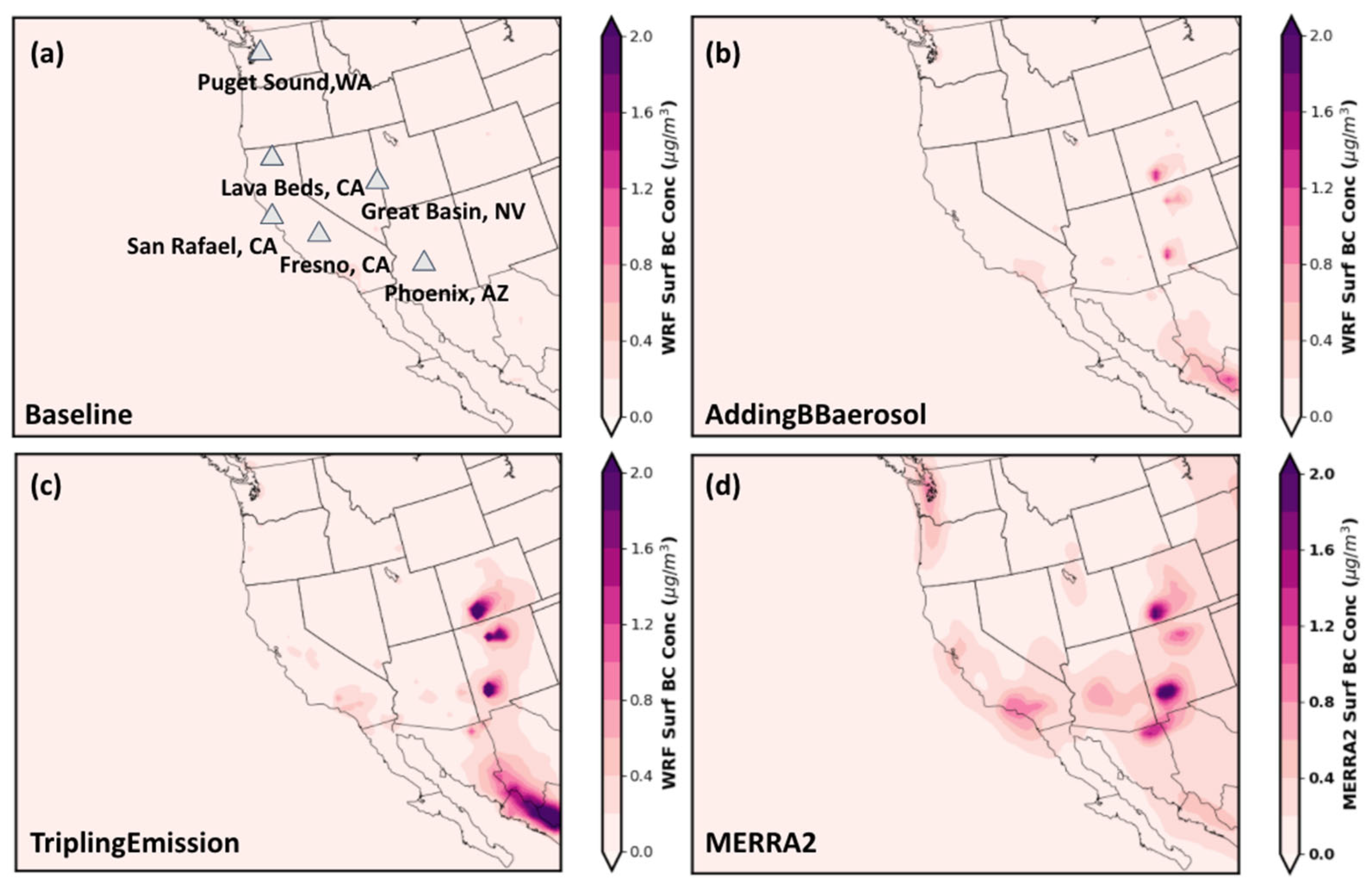
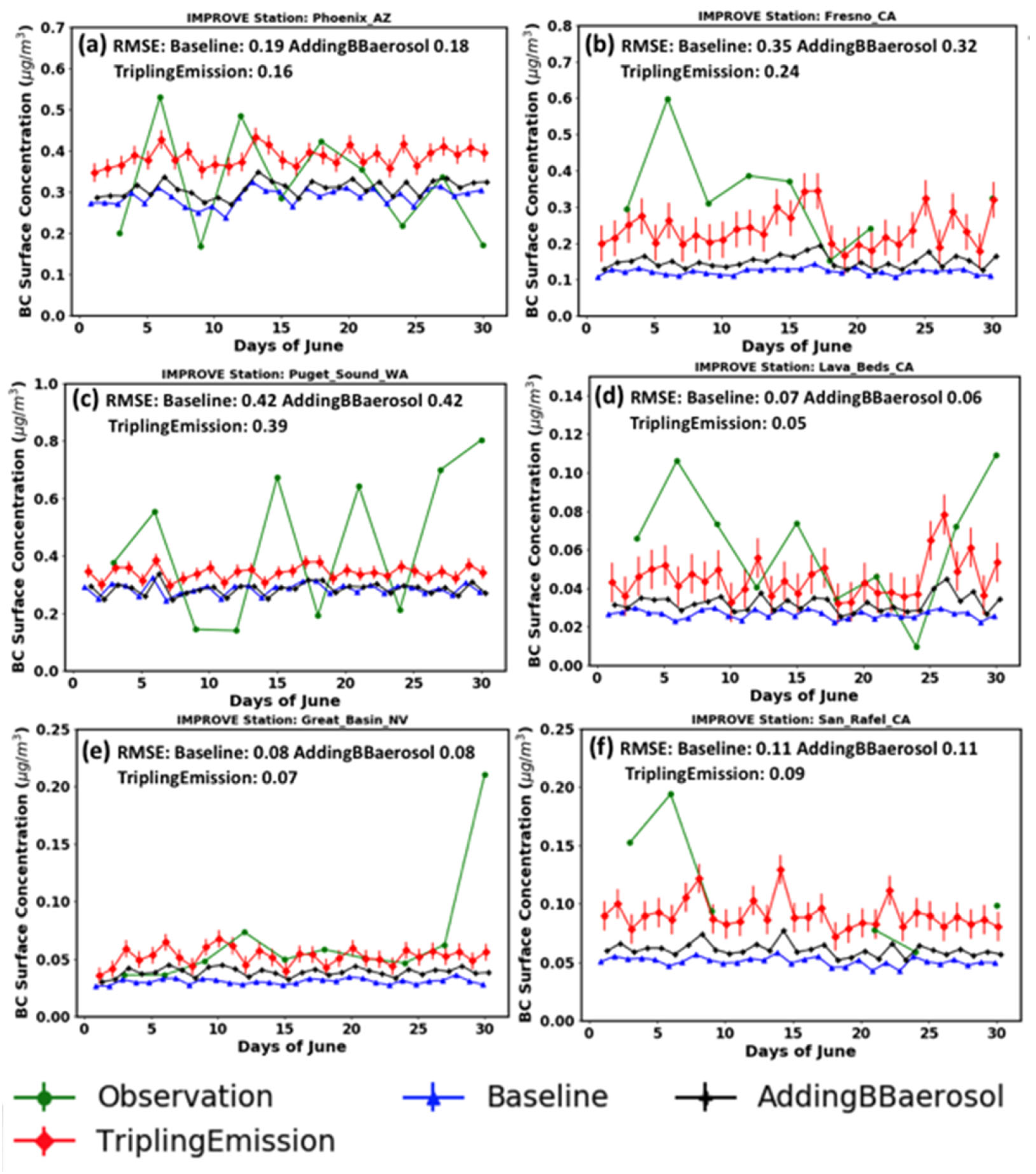
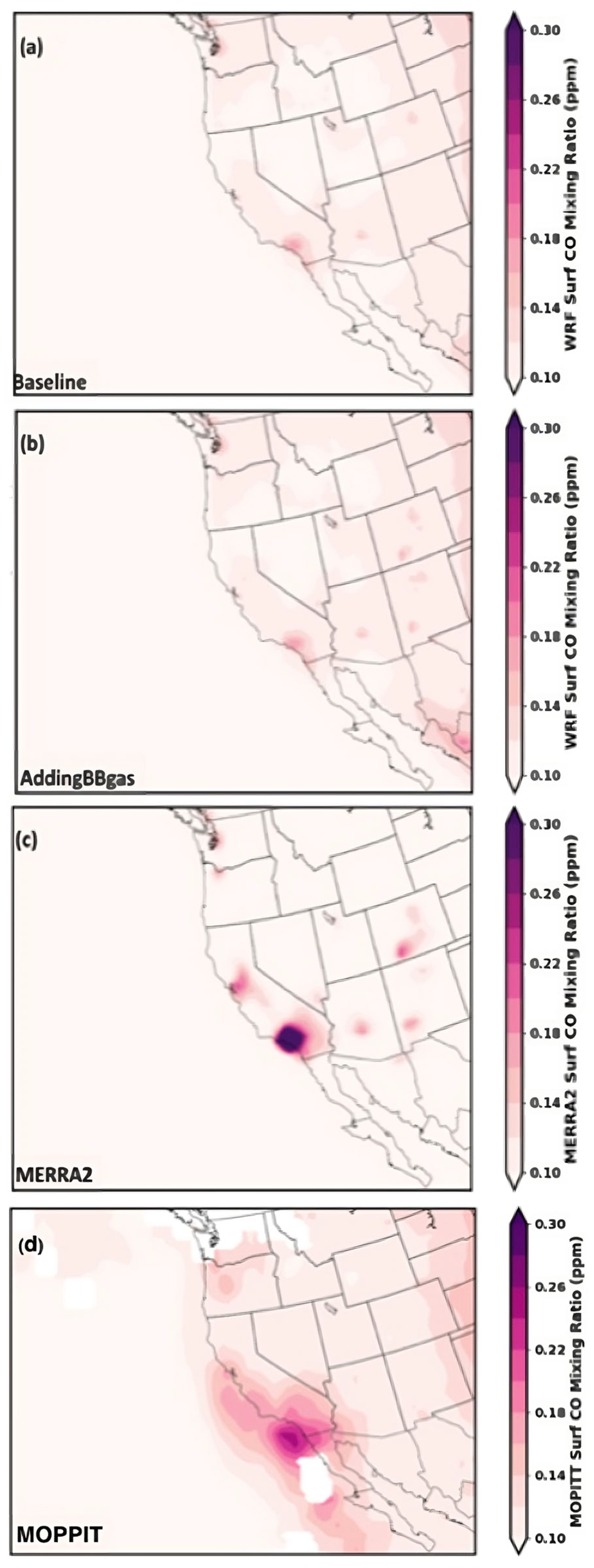
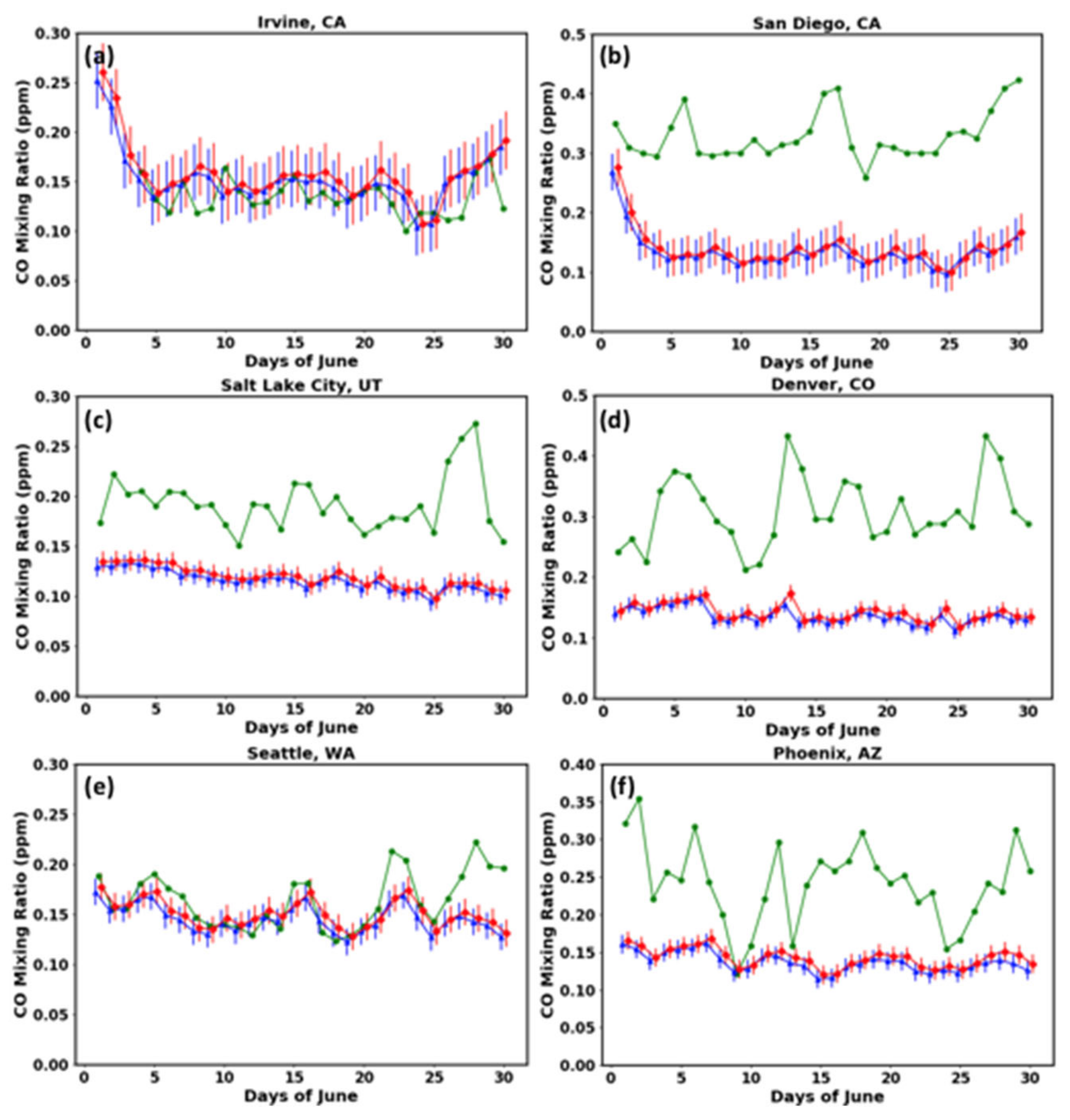
4.2.2. Improvements in Primary Species of BC and CO

In addition to the AOD, we also evaluated the surface mass concentrations of individual species. Figure 7 shows the surface BC concentrations from each model modification compared with the data from MERRA-2. For BC, the baseline simulation completely missed the hotspots shown in MERRA-2, with only slight plume footprints found near the Los Angeles metropolitan area. After enabling the biomass burning emissions of aerosols (AddingBBaerosol), the spatial distribution of BC shows patterns that are more consistent with the MERRA-2 observations. Performance was further improved in the TriplingEmission run. Under this configuration, the simulated BC is comparable to the MERRA-2 results, with only some overestimation of the BC concentrations in Mexico. These sensitivity studies indicate that biomass burning emissions of BC from FINN may be underestimated in the western United States and Mexico.

Figure 8 shows the station-by-station comparison between the simulated and observed surface BC concentrations at six IMPROVE sites (location shown in Figure 7a). Generally, the observed BC is higher than the simulated values, especially for the baseline simulation; keep in mind that the IMPROVE network reports data on a 3-day basis (see Section 2). Further chemistry and emissions enhancements help mitigate the bias in the simulated results. Most of the observed daily BC values are within the day-to-day variability in the simulations, indicating that our simulation performs reasonably well over most sites. Puget Sound, Washington, is the only site where the simulations failed to capture the observations entirely. The large 3-day variability in the observational data exceeds the range of model uncertainty, yet the improved emissions-enhanced (AddingSOC/TriplingEmission) simulations yield results closer to the observed values.

For the primarily emitted chemicals, we also supplied emissions of gas-phase species. This improvement is shown in Figure 9 using CO as an example. In Figure 9b, CO emitted by biomass burning emerges from New Mexico and the southwestern part of Colorado. These hotspots of high CO mixing ratios coincide with the hotspots of high BC concentrations shown in Figure 7, indicating that biomass burning dominates the contributions over these regions. After adding the biomass burning emissions of gas species, the spatial pattern of the CO mixing ratios becomes similar to that of the MERRA-2 products shown in Figure 9c and MOPITT in Figure 9d. The MOPITT is largely similar to the MERRA-2 products, and, therefore, we believe that MERRA-2 should be considered trustworthy when capturing large-scale patterns. However, the model still underestimates the MERRA-2 values. For surface observations of CO, we compared the daily mixing ratios to the observations (Figure 10) at the same sites that are used for the temperature evaluation (shown in Figure 3).

For Irvine, California, and Seattle, Washington, the simulated CO mixing ratios match the observations very well (mean biases < 0.05 ppm). The results are less accurate in Salt Lake City, Utah, and Phoenix, Arizona. The simulated levels suffer from low biases of 0.1 to 0.2 ppm in these two cities; however, the daily results in both cities see improvements that are closer to the daily observations after the implementation of AddingBBgas. Over San Diego, California, and Denver, Colorado, the simulated results were rather poor. The low biases are generally between 0.2 and 0.3 ppm. As for the surface temperature, the low biases for Denver and Salt Lake City are considered to be topography-induced. Because both cities are surrounded by nearby mountainous areas, the CO levels tend to be diluted due to the mixing of urban emissions with cleaner mountainous air. Thus, when conducting spatial averaging, these regions will suffer from low biases.

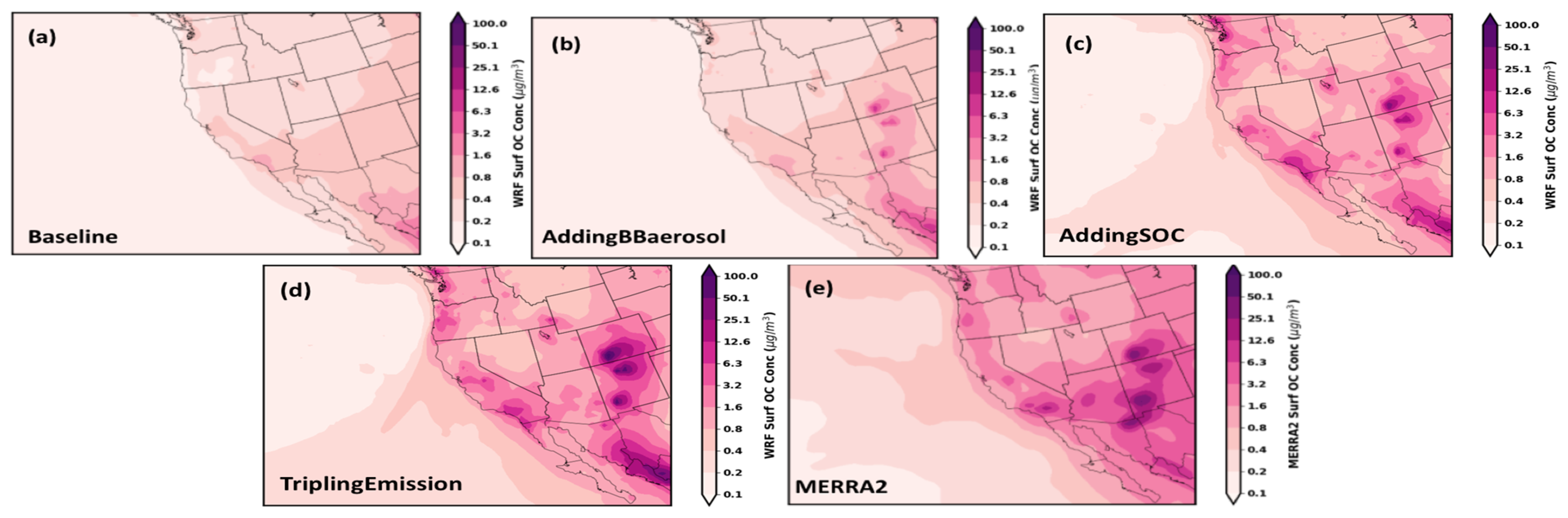
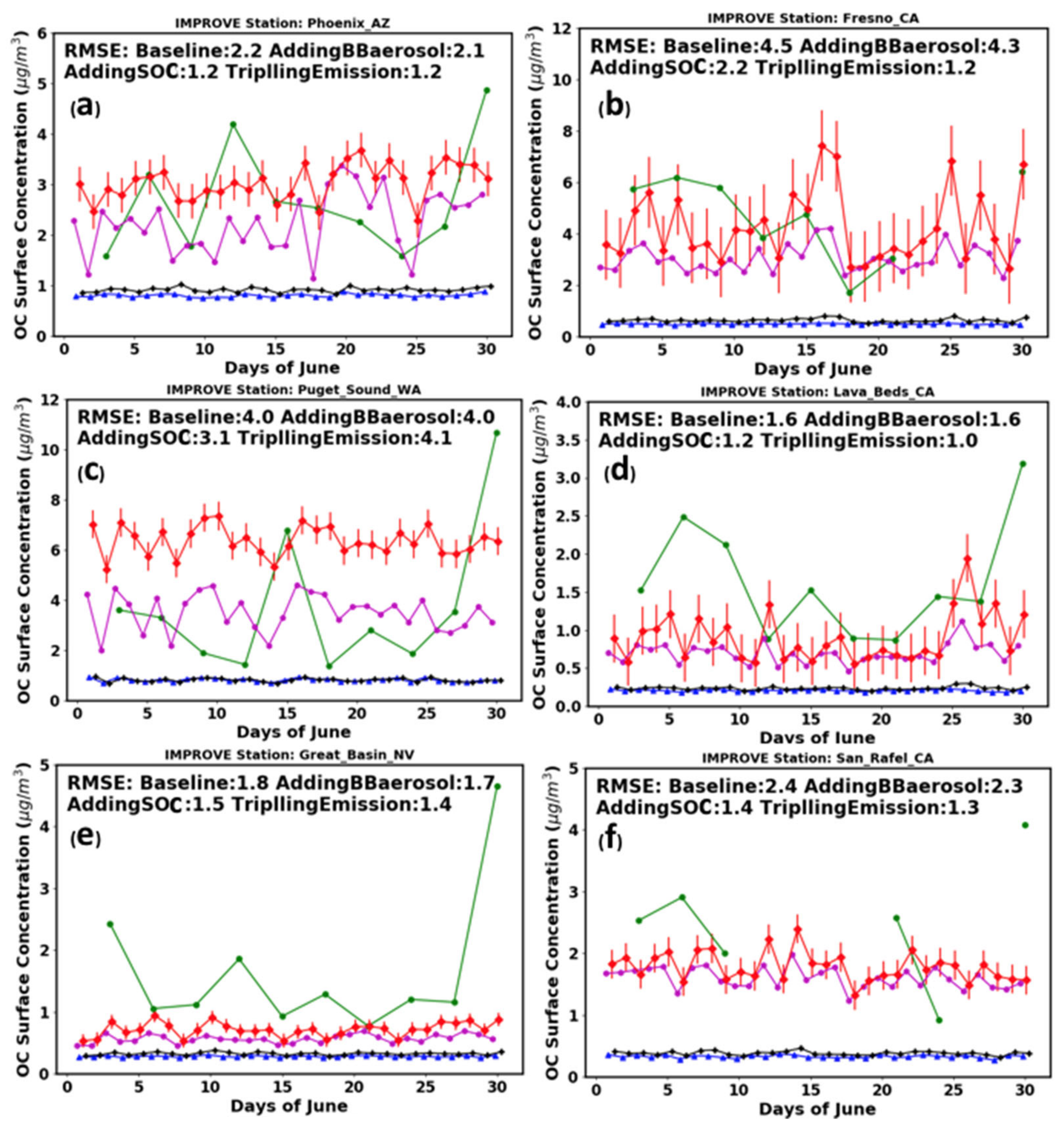
4.2.3. Improvements of OC (POC and SOC)

Similar to BC, the simulated OC concentrations and spatial distributions underwent step-by-step improvements due to the modifications mentioned above. Furthermore, OC consists of both primary and secondary sources, so we added one more case of VOC-to-SOC conversion (AddingSOC) when comparing the OC against observations or reanalysis products; Figure 11 shows this improvement spatially (in log scale). Like that of BC, the OC spatial pattern is significantly affected by the biomass burning locations. After AddingBBaerosol, regions close to areas of strong biomass burning emissions become spatially more consistent with the data from the MERRA-2 products. Although we see some improvements after adding the primary OC, the discrepancy between the simulation (Figure 11b) and reanalysis (Figure 11e) remains large. Such differences are significantly reduced by implementing the VOC-to-SOC conversions (Figure 11c). In the cases with TriplingEmission initiated, the simulated total OC is estimated to be 0.68 μg/m³ (22%) larger than that of the MERRA-2 products for the United States on average.

When comparing the simulated OC to observations from the IMPROVE stations, the modified model versions have much better performance than the baseline run (Figure 12), with a reduced root-mean-square error (RMSE) of 2.43 μg/m³. For most stations, the observed OC is close to the output from the AddingSOC and TriplingEmission runs. Two stations (Lava Beds, California, and Great Basin, Nevada) have even higher observed OC values, albeit only slightly higher than that of the TriplingEmission run. On most days, the observations fall within the range of the simulation results, indicating that the enhanced model implementation successfully captures the overall OC concentration levels.

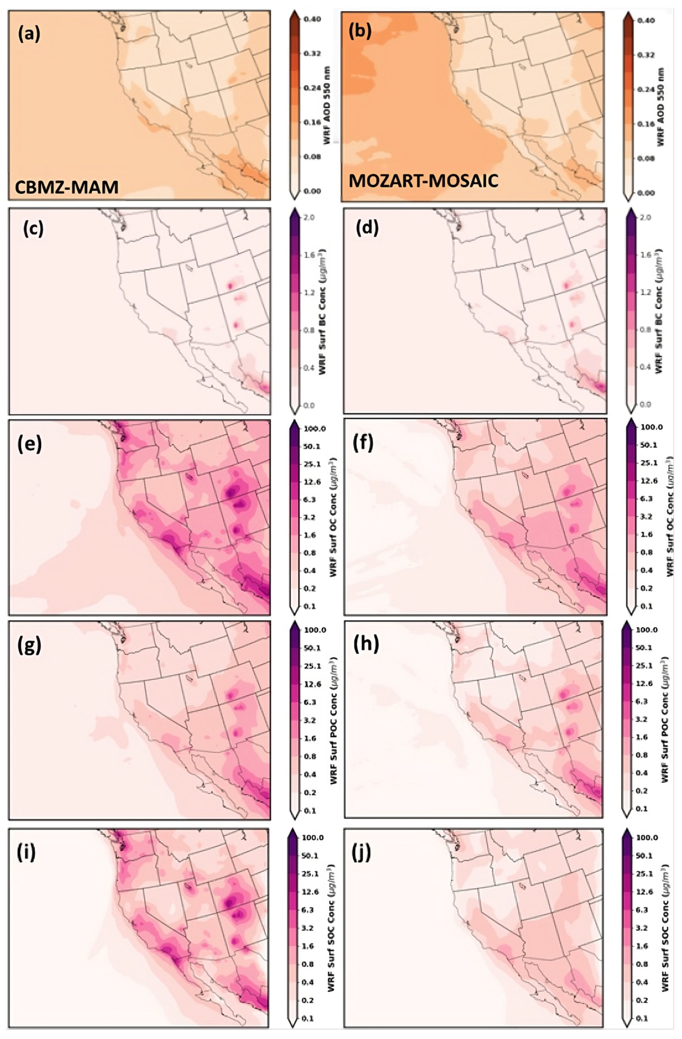
4.3. Comparison with MOZART-MOSAIC

One question we aim to answer here is how the CBMZ-MAM3 simulation performs compared to the more comprehensive MOZART-MOSAIC configuration. Note that the CBMZ-MAM3 chemistry suite demands 2.5-times fewer computational core hours compared to the MOZART-MOSAIC simulations. Thus, we also evaluated the BC, OC, and AOD results for the MOZART-MOSAIC simulation (Figure 13); to maintain consistency, we did not adjust the emissions levels in either the CBMZ-MAM3 or the MOZART-MOSAIC runs.

For the AOD (first row of Figure 13), the two suites have comparable performance in terms of absolute magnitude, but we can still identify better spatial agreement for the CBMZ-MAM3 scheme compared to the MOZART-MOSAIC scheme. For BC (second row of Figure 12), MOZART-MOSAIC yields concentration levels comparable to those of the CBMZ-MAM3 simulations. For OC (third row of Figure 12), MOZART-MOSAIC has much lower values than the CBMZ-MAM3 results. When using the MERRA-2 products as the benchmark (Figure 11 and Figure 13), the improved CBMZ-MAM3 produced better results despite being a less sophisticated chemistry scheme.

The major difference in OC between the two sites comes from the SOC treatment. Figure 13 (bottom two rows) compares both the primary and secondary OC between MOZART-MOSAIC and CBMZ-MAM3. For the primary OC, two chemistry suites show comparable results in terms of both the spatial pattern and magnitude; however, only the improved CBMZ-MAM3 simulation is capable of identifying SOC concentration hotspots, while MOZART-MOSAIC fails to do so. One plausible explanation for this is that the added VOC species in MAM3 include hydroxyacetone, which dominates the VOC-to-SOC conversion, while the current MOZART-MOSAIC configuration does not incorporate this species and its conversion to SOAs.

Despite the dominating role the chemistry suite may play, the simulated differences between WRF-CAM5 with CBMZ-MAM3 chemistry and WRF-Chem with MOZART-MOSAIC chemistry should not be attributed to chemistry suite selection only. This is because the different microphysics and other physical schemes in these two sets of simulations can also lead to the different diffusion and transport of chemical species. However, the main goal of comparing with the MOZART-MOSAIC simulation is to demonstrate a similar performance between these two model setups despite a much higher computational efficiency using WRF-CAM5 (our model here).

In addition to observations and reanalysis products, our results are further compared to other simulations, Jaffe et al. [87] and Spracklen et al. [88], for similarity. For example, our simulated CO mixing ratio for AddingBBgas in the northwestern US (Figure 9 and Figure 10) aligns with the results of Jaffe et al. [87], who used the Naval Research Laboratory aerosol analysis and prediction system. Furthermore, our TriplingEmission results are largely consistent with Jaffe et al. [87]. Additionally, the organic carbon (OC) values in Spracklen et al. [88]. agree with our findings in Figure 11, demonstrating similar orders of magnitude. These results were obtained using GEOS-Chem global 3-D CTM simulations. Therefore, we conclude that the overall geospatial patterns are largely consistent.

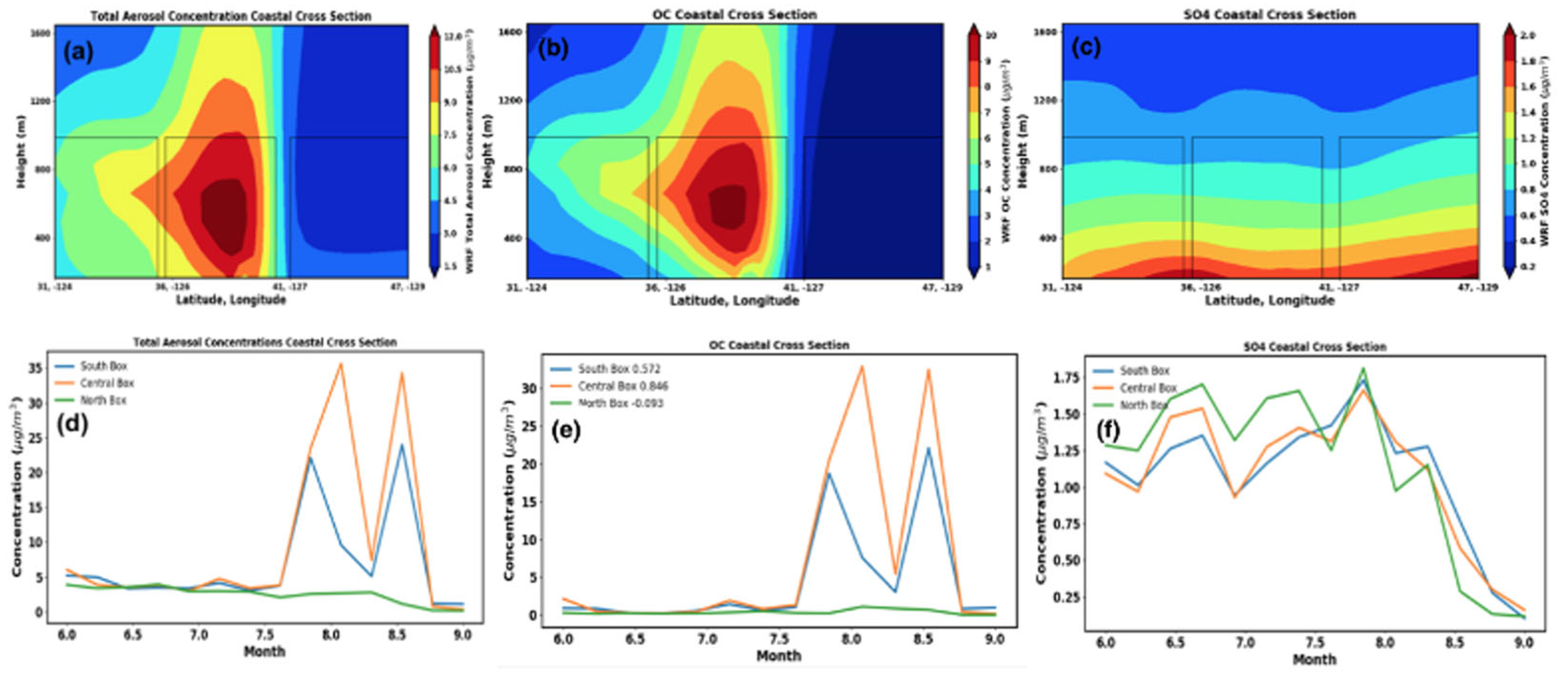
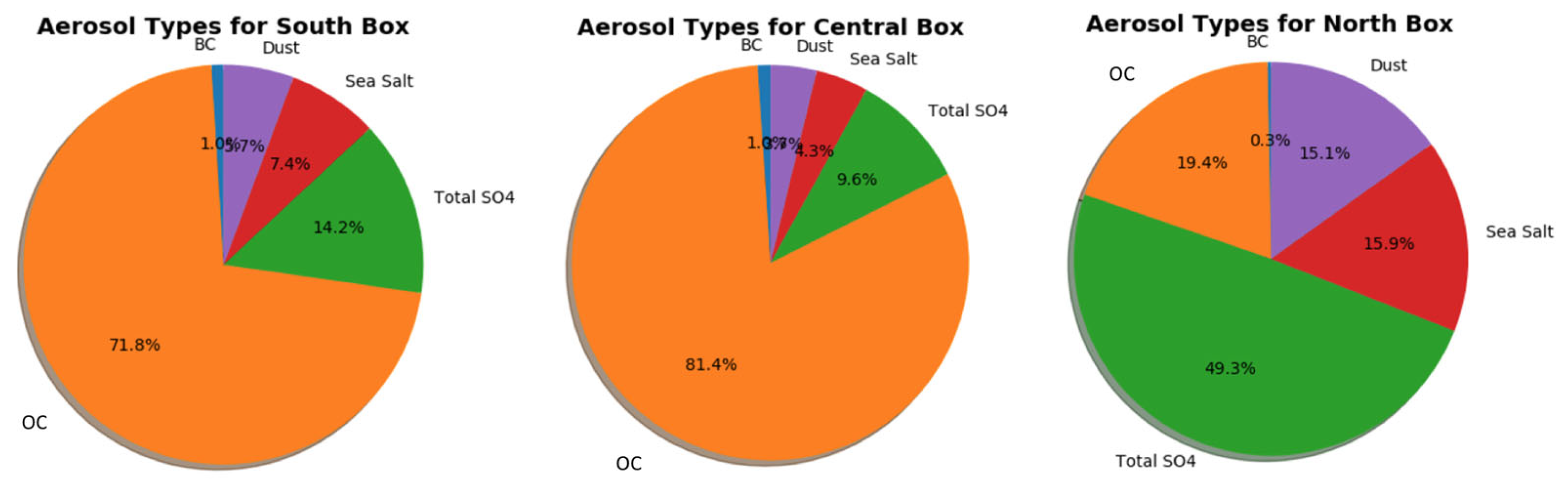
4.4. Off-Coast Aerosols

Finally, we demonstrate a potential application of this improved model by showing off-coast aerosol simulations near California. Here, we break the off-coast areas into three boxes representing north, central, and south boxes (Figure 14) with their vertical profiles and time series depicted.

Figure 14a shows the total aerosol concentration in the region, with the central box showing a dominant level followed by the south box. The north box, on the contrary, has much lower aerosol concentrations compared to both the central and south boxes. In Figure 14b,c, we present the accompanied OC and sulfates concentrations, and the rationale behind showing these two species is shown in Figure 15, as OC and sulfates are the two dominant species in this region.

OC has very similar vertical distributions and time series compared to the total aerosol concentrations (Figure 14), which is expected as OC dominates the aerosol composition in both the south and central Box (Figure 15). For SO₄ levels, all three boxes share similar total concentrations.

When evaluating the time series of aerosols, the temporal pattern of total aerosol is largely similar to the OC’s pattern, with two episodic events taking place between July and September. In contrast, the SO₄ peaks in the early periods of this simulation (from June to August) and drops significantly afterward. In addition, the time series of SO₄ has very similar spatial patterns across all three boxes while the OC exhibits biased temporal patterns (heavily dominated by the central and north Boxes) for its time series. Such a discrepancy indicates that these aerosols could be transported from different episodic events with different origins.

5. Conclusions

WRF-CAM5 is widely used in many atmospheric chemistry applications such as air quality, chemistry, and climate interactions [26]. In this study, we enhanced the chemistry suite in WRF-CAM5 for simulations of biomass burning trace gases and secondary aerosol formation by modifying both the CBMZ and MAM3 modules and any accompanying modules or registries (i.e., the plume rise, emissions-driver, and chemistry-driver modules). In total, we performed four progressive modifications to understand the relative importance of these processes: (1) adding the model capability to incorporate the biomass burning emitted aerosols in MAM (AddingBBaerosol); (2) adding the model capability to incorporate the biomass burning emitted gases in CBMZ (AddingBBgas); (3) implementing VOC-to-SOC conversions (AddingSOC); and (4) increasing the anthropogenic and biomass burning emissions over the western US by a factor of three (TriplingEmission).

The simulated results demonstrate step-by-step improvements after introducing each modification. In general, when compared to observations, the model performance follows the order of TriplingEmission > AddingSOC > AddingBBaerosol > baseline. These improvements lead to not only more spatial consistency but also better agreement with the observations. Both simulated aerosol concentrations and gas-phase species and AOD at 550 nm showed significant improvements after the model modifications.

Species-wise, both BC and OC have improved accuracies with an RMSE reduction of 0.5 μg/m³ (31% less) for BC and 2.4 μg/m³ (58% less) for OC. We also identified considerable improvements for OC after introducing the secondary VOC-to-SOC processes and emissions enhancements. This study suggests that the low bias of the current version (baseline) comes from both model deficiencies (no biomass burning emissions and VOC-to-SOC conversions) and underestimated biomass burning emissions.

Furthermore, we also compared our results with a more comprehensive MOZART-MOSAIC setup. For directly emitted species (e.g., BC), both models yield comparable results. For species involving secondary processes (e.g., OC), CBMZ-MAM3 agrees better with the MERRA-2 reanalysis data. It is noteworthy that the MOZART-MOSAIC chemistry suite is generally considered to be more sophisticated and requires 2.5 times more computational core hours.

Our results suggest that the improved WRF-CAM5–CBMZ-MAM3 can produce reasonable simulations of biomass burning aerosols over the western US and eastern North Pacific while maintaining a low computational cost. This modeling capability with both accuracy and computational efficiency could be used for studying the long-term trends (e.g., in the last 30 years) of biomass burning aerosols and trace gases resulting from the increased wildfires over the western US [89], and their influences on the regional climate at a higher resolution than global climate models. However, we found that there is a substantial underestimation in both biomass burning and anthropogenic emissions over this region, consistent with previous studies. An increase in the emissions by a factor of three is needed in the present study to match the regional AOD observations from either ground-based or satellite remote sensing independent of the selected chemistry-aerosol scheme (i.e., CBMZ-MAM3 vs. MOZART-MOSAIC).

Further investigations of the biomass burning emissions and related processes in this region, e.g., emissions from small or smoldering fires and injection height of moderate and large fires, may help resolve the model’s low bias. In addition to the emissions, enhanced aerosol wet removal resulting from the increase in model horizontal resolution [90] might also contribute to the underestimated AOD, and re-tuning the aerosol wet removal efficiency might be needed when the model resolution is refined, e.g., from the global CAM5 model to the WRF-CAM5.

Lastly, one may challenge the notion that the exponential growth in computational power could render efficient chemistry representation in regional models unnecessary. However, we believe that there will always be a desire for simulations with higher spatial and temporal resolution, as well as longer periods. Furthermore, high-performance computing is not a luxury accessible to everyone who seeks it. Therefore, we aim to empower those who wish to conduct climate–chemistry studies by providing them with the best accessible tools. Future studies may consider implementing and quantifying the upgraded CBMZ-MAM3 chemistry suites for other regional aerosol and climate simulations and/or for different time periods (seasons). Furthermore, this paper illustrated how to add biomass burning into WRF-CAM5 models and supplied a pathway for VOC-to-SOC conversion. Future model developers are encouraged to further validate their results before publishing the products.

References

1. Brasseur, G.P.; Jacob, D.J. Modeling of Atmospheric Chemistry; Cambridge University Press: Cambridge, UK, 2017. [Google Scholar]
2. Skamarock, W.C.; Klemp, J.B.; Dudhia, J.; Gill, D.O.; Barker, D.M.; Wang, W.; Powers, J.G. A Description of the Advanced Research WRF Version 2; NCAR Tech (p. 88). Note NCAR/TN-4681STR; National Center for Atmospheric Research: Boulder, CO, USA, 2005. [Google Scholar]
3. Grell, G.A.; Peckham, S.E.; Schmitz, R.; McKeen, S.A.; Frost, G.; Skamarock, W.C.; Eder, B. Fully coupled “online” chemistry within the WRF model. Atmos. Environ. 2005, 39, 6957–6975. [Google Scholar] [CrossRef]
4. Kumar, R.; Ghude, S.D.; Biswas, M.; Jena, C.; Alessandrini, S.; Debnath, S.; Kulkarni, S.; Sperati, S.; Soni, V.K.; Nanjundiah, R.S.; et al. Enhancing Accuracy of Air Quality and Temperature Forecasts During Paddy Crop Residue Burning Season in Delhi Via Chemical Data Assimilation. J. Geophys. Res. Atmos. 2020, 125, e2020JD033019. [Google Scholar] [CrossRef]
5. Kumar, R.; Barth, M.C.; Pfister, G.G.; Delle Monache, L.; Lamarque, J.F.; Archer-Nicholls, S.; Tilmes, S.; Ghude, S.D.; Wiedinmyer, C.; Naja, M.; et al. How will air quality change in South Asia by 2050? J. Geophys. Res. Atmos. 2018, 123, 1840–1864. [Google Scholar] [CrossRef]
6. Xu, Y.; Wu, X.; Kumar, R.; Barth, M.; Diao, C.; Gao, M.; Lin, L.; Jones, B.; Meehl, G.A. Substantial Increase in the Joint Occurrence and Human Exposure of Heatwave and High-PM Hazards Over South Asia in the Mid-21st Century. AGU Adv. 2020, 1, e2019AV000103. [Google Scholar] [CrossRef] [Green Version]
7. Wu, X.; Xu, Y.; Kumar, R.; Barth, M. Separating Emission and Meteorological Drivers of Mid-21st-Century Air Quality Changes in India Based on Multi year Global-Regional Chemistry-Climate Simulations. J. Geophys. Res. Atmos. 2019, 124, 13420–13438. [Google Scholar] [CrossRef]
8. Zhang, Y.; Wen, X.Y.; Jang, C.J. Simulating chemistry–aerosol-cloud–radiation–climate feedbacks over the continental US using the online-coupled Weather Research Forecasting Model with chemistry (WRF/Chem). Atmos. Environ. 2010, 44, 3568–3582. [Google Scholar] [CrossRef]
9. Feng, Y.; Kotamarthi, V.R.; Coulter, R.; Zhao, C.; Cadeddu, M. Radiative and thermodynamic responses to aerosol extinction profiles during the pre-monsoon month over South Asia. Atmos. Meas. Tech. 2016, 16, 247–264. [Google Scholar] [CrossRef] [Green Version]
10. He, C.; Flanner, M.G.; Chen, F.; Barlage, M.; Liou, K.-N.; Kang, S.; Ming, J.; Qian, Y. Black carbon-induced snow albedo reduction over the Tibetan Plateau: Uncertainties from snow grain shape and aerosol–snow mixing state based on an updated SNICAR model. Atmos. Meas. Tech. 2018, 18, 11507–11527. [Google Scholar] [CrossRef] [Green Version]
11. Grell, G.; Freitas, S.R.; Stuefer, M.; Fast, J. Inclusion of biomass burning in WRF-CAM5: Impact of wildfires on weather forecasts. Atmos. Chem. Phys. 2011, 11, 5289–5303. [Google Scholar] [CrossRef] [Green Version]
12. Galin, V.Y.; Smyshlyaev, S.P.; Volodin, E.M. Combined chemistry-climate model of the atmosphere. Izv. Atmos. Ocean. Phys. 2007, 43, 399–412. [Google Scholar] [CrossRef]
13. Barnard, J.C.; Fast, J.D.; Paredes-Miranda, G.; Arnott, W.P.; Laskin, A. Evaluation of the WRF-CAM5 “Aerosol Chemical to Aerosol Optical Properties” Module using data from the MILAGRO campaign. Atmos. Chem. Phys. 2010, 10, 7325–7340. [Google Scholar] [CrossRef] [Green Version]
14. Chin, M.; Rood, R.; Lin, S.-J.; Müller, J.-F.; Thompson, A.M. Atmospheric sulfur cycle simulated in the global model GOCART: Model description and global properties. J. Geophys. Res. Atmos. 2000, 105, 24671–24687. [Google Scholar] [CrossRef]
15. Emmons, L.K.; Walters, S.; Hess, P.G.; Lamarque, J.-F.; Pfister, G.G.; Fillmore, D.; Granier, C.; Guenther, A.; Kinnison, D.; Laepple, T.; et al. Description and evaluation of the Model for Ozone and Related chemical Tracers, version 4 (MOZART-4). Geosci. Model Dev. 2010, 3, 43–67. [Google Scholar] [CrossRef] [Green Version]
16. Zaveri, R.A.; Easter, R.C.; Fast, J.D.; Peters, L.K. Model for Simulating Aerosol Interactions and Chemistry (MOSAIC). J. Geophys. Res. Atmos. 2008, 113, D13. [Google Scholar] [CrossRef]
17. Peckham, S.; Grell, G.A.; McKeen, S.A.; Barth, M.; Pfister, G.; Wiedinmyer, C.; Fast, J.D.; Gustafson, W.I.; Zaveri, R.A.; Easter, R.C.; et al. WRF/Chem Version 3.3 User’s Guide; NOAA Technical Memo; US Department of Commerce, National Oceanic and Atmospheric Administration, Oceanic and Atmospheric Research Laboratories: Boulder, CO, USA, 2012; pp. 1–99. [Google Scholar]
18. Phoenix, D.B.; Homeyer, C.R.; Barth, M.C. Sensitivity of simulated convection-driven stratosphere-troposphere exchange in WRF-Chem to the choice of physical and chemical parameterization. Earth Space Sci. 2017, 4, 454–471. [Google Scholar] [CrossRef] [Green Version]
19. Shrivastava, M.; Fast, J.; Easter, R.; Gustafson, W.I., Jr.; Zaveri, R.A.; Jimenez, J.L.; Saide, P.; Hodzic, A. Modeling organic aerosols in a megacity: Comparison of simple and complex representations of the volatility basis set approach. Atmos. Chem. Phys. 2011, 11, 6639–6662. [Google Scholar] [CrossRef] [Green Version]
20. Emmerson, K.M.; Evans, M.J. Comparison of tropospheric gas-phase chemistry schemes for use within global models. Atmos. Meas. Tech. 2009, 9, 1831–1845. [Google Scholar] [CrossRef] [Green Version]
21. Bey, I.; Jacob, D.J.; Yantosca, R.M.; Logan, J.A.; Field, B.D.; Fiore, A.M.; Li, Q.; Liu, H.Y.; Mickley, L.J.; Schultz, M.G. Global modeling of tropospheric chemistry with assimilated meteorology: Model description and evaluation. J. Geophys. Res. Atmos. 2001, 106, 23073–23095. [Google Scholar] [CrossRef] [Green Version]
22. Liu, X.; Easter, R.C.; Ghan, S.J.; Zaveri, R.; Rasch, P.; Shi, X.; Lamarque, J.-F.; Gettelman, A.; Morrison, H.; Vitt, F.; et al. Toward a minimal representation of aerosols in climate models: Description and evaluation in the Community Atmosphere Model CAM5. Geosci. Model Dev. 2012, 5, 709–739. [Google Scholar] [CrossRef] [Green Version]
23. Peckham, S.E.; Grell, G.A.; McKeen, S.A.; Ahmadov, R.; Wong, K.Y.; Barth, M.; Ghan, S.J. WRF-CAM5 Version 3.8. 1 User’s Guide; National Oceanic and Atmospheric Administration: Wasington, DC, USA, 2017.
24. Ma, P.L.; Rasch, P.J.; Fast, J.D.; Easter, R.C.; Gustafson, W.I., Jr.; Liu, X.; Ghan, S.J.; Singh, B. Assessing the CAM5 physics suite in the WRF-CAM5 model: Implementation, resolution sensitivity, and a first evaluation for a regional case study. Geosci. Model Dev. 2014, 7, 755. [Google Scholar] [CrossRef] [Green Version]
25. He, J.; Zhang, Y.; Wang, K.; Chen, Y.; Leung, L.R.; Fan, J.; Li, M.; Zheng, B.; Zhang, Q.; Duan, F.; et al. Multi-year application of WRF-CAM5 over East Asia-Part I: Comprehensive evaluation and formation regimes of O3 and PM2.5. Atmos. Environ. 2017, 165, 122–142. [Google Scholar] [CrossRef]
26. Zhang, Y.; Zhang, X.; Wang, K.; He, J.; Leung, L.R.; Fan, J.; Nenes, A. Incorporating an advanced aerosol activation pa-rameterization into WRF-CAM5: Model evaluation and parameterization intercomparison. J. Geophys. Res. Atmos. 2015, 120, 6952–6979. [Google Scholar] [CrossRef]
27. Painemal, D.; Minnis, P.; Nordeen, M. Aerosol variability, synoptic-scale processes, and their link to the cloud microphysics over the northeast Pacific during MAGIC. J. Geophys. Res. Atmos. 2015, 120, 5122–5139. [Google Scholar] [CrossRef]
28. Morrison, H.; Gettelman, A. A New Two-Moment Bulk Stratiform Cloud Microphysics Scheme in the Community Atmosphere Model, Version 3 (CAM3). Part I: Description and Numerical Tests. J. Clim. 2008, 21, 3642–3659. [Google Scholar] [CrossRef]
29. Morrison, H.; Thompson, G.; Tatarskii, V. Impact of Cloud Microphysics on the Development of Trailing Stratiform Precipitation in a Simulated Squall Line: Comparison of One- and Two-Moment Schemes. Mon. Weather. Rev. 2009, 137, 991–1007. [Google Scholar] [CrossRef] [Green Version]
30. Kanakidou, M.; Seinfeld, J.H.; Pandis, S.N.; Barnes, I.; Dentener, F.J.; Facchini, M.C.; Van Dingenen, R.; Ervens, B.; Nenes, A.; Nielsen, C.J.; et al. Organic aerosol and global climate modelling: A review. Atmos. Chem. Phys. 2005, 5, 1053–1123. [Google Scholar] [CrossRef] [Green Version]
31. Tsigaridis, K.; Kanakidou, M. Secondary organic aerosol importance in the future atmosphere. Atmos. Environ. 2007, 41, 4682–4692. [Google Scholar] [CrossRef]
32. Camredon, M.; Aumont, B.; Lee-Taylor, J.; Madronich, S. The SOA/VOC/NO x system: An explicit model of secondary organic aerosol formation. Atmos. Chem. Phys. 2007, 7, 5599–5610. [Google Scholar] [CrossRef] [Green Version]
33. Skamarock, W.C.; Klemp, J.B. A time-split nonhydrostatic atmospheric model for weather research and forecasting ap-plications. J. Comput. Phys. 2008, 227, 3465–3485. [Google Scholar] [CrossRef]
34. Iacono, M.J.; Delamere, J.S.; Mlawer, E.J.; Shephard, M.W.; Clough, S.A.; Collins, W.D. Radiative forcing by long-lived greenhouse gases: Calculations with the AER radiative transfer models. J. Geophys. Res. Atmos. 2008, 113, D13103. [Google Scholar] [CrossRef]
35. Tewari, M.; Chen, F.; Wang, W.; Dudhia, J.; LeMone, M.A.; Mitchell, K.; Ek, M.; Gayno, G.; Wegiel, J.; Cuenca, R.H. Implementation and verification of the unified NOAH land surface model in the WRF model. In Proceedings of the 20th Conference on Weather Analysis and Forecasting/16th Conference on Numerical Weather Prediction, Seattle, WA, USA, 10–15 January 2004; American Meteorological Society: Boston, MA, USA, 2004; Volume 1115. [Google Scholar]
36. Zaveri, R.A.; Peters, L.K. A new lumped structure photochemical mechanism for large-scale applications. J. Geophys. Res. Atmos. 1999, 104, 30387–30415. [Google Scholar] [CrossRef]
37. Park, S.; Bretherton, C.S. The University of Washington Shallow Convection and Moist Turbulence Schemes and Their Impact on Climate Simulations with the Community Atmosphere Model. J. Clim. 2009, 22, 3449–3469. [Google Scholar] [CrossRef]
38. Hong, S.-Y.; Noh, Y.; Dudhia, J. A New Vertical Diffusion Package with an Explicit Treatment of Entrainment Processes. Mon. Weather. Rev. 2006, 134, 2318–2341. [Google Scholar] [CrossRef] [Green Version]
39. Wild, O.; Zhu, X.; Prather, M.J. Fast-J: Accurate Simulation of In- and Below-Cloud Photolysis in Tropospheric Chemical Models. J. Atmos. Chem. 2000, 37, 245–282. [Google Scholar] [CrossRef]
40. Tie, X.; Madronich, S.; Walters, S.; Edwards, D.P.; Ginoux, P.; Mahowald, N.; Zhang, R.; Lou, C.; Brasseur, G. Assessment of the global impact of aerosols on tropospheric oxidants. J. Geophys. Res. Atmos. 2005, 110, D03204. [Google Scholar] [CrossRef] [Green Version]
41. Lamarque, J.-F.; Emmons, L.K.; Hess, P.G.; Kinnison, D.E.; Tilmes, S.; Vitt, F.; Heald, C.L.; Holland, E.A.; Lauritzen, P.H.; Neu, J.; et al. CAM-chem: Description and evaluation of interactive atmospheric chemistry in the Community Earth System Model. Geosci. Model Dev. 2012, 5, 369–411. [Google Scholar] [CrossRef] [Green Version]
42. US Environmental Protection Agency 2014 National Emissions Inventory, version 2 Technical Support Document. 2018. Available online: https://www.epa.gov/sites/default/files/2018-07/documents/nei2014v2_tsd_05jul2018.pdf (accessed on 20 June 2023).
43. Janssens-Maenhout, G.; Crippa, M.; Guizzardi, D.; Dentener, F.; Muntean, M.; Pouliot, G.; Keating, T.; Zhang, Q.; Kurokawa, J.; Wankmüller, R.; et al. HTAP_v2.2: A mosaic of regional and global emission grid maps for 2008 and 2010 to study hemispheric transport of air pollution. Atmos. Meas. Tech. 2015, 15, 11411–11432. [Google Scholar] [CrossRef] [Green Version]
44. Wiedinmyer, C.; Akagi, S.K.; Yokelson, R.J.; Emmons, L.K.; Al-Saadi, J.A.; Orlando, J.J.; Soja, A.J. The Fire INventory from NCAR (FINN): A high resolution global model to estimate the emissions from open burning. Geosci. Model Dev. 2011, 4, 625–641. [Google Scholar] [CrossRef] [Green Version]
45. Guenther, A.; Karl, T.; Harley, P.; Wiedinmyer, C.; Palmer, P.I.; Geron, C. Estimates of global terrestrial isoprene emissions using MEGAN (Model of Emissions of Gases and Aerosols from Nature). Atmos. Chem. Phys. 2006, 6, 3181–3210, Corrected in Atmos. Chem. Phys. 2006, 6, 3181–3210. [Google Scholar] [CrossRef] [Green Version]
46. Gelaro, R.; McCarty, W.; Suárez, M.J.; Todling, R.; Molod, A.; Takacs, L.; Randles, C.A.; Darmenov, A.; Bosilovich, M.G.; Reichle, R.; et al. The Modern-Era Retrospective Analysis for Research and Applications, Version 2 (MERRA-2). J. Clim. 2017, 30, 5419–5454. [Google Scholar] [CrossRef]
47. Randles, C.A.; Da Silva, A.M.; Buchard, V.; Colarco, P.R.; Darmenov, A.; Govindaraju, R.; Smirnov, A.; Holben, B.; Ferrare, R.; Hair, J.; et al. The MERRA-2 Aerosol Reanalysis, 1980 Onward. Part I: System Description and Data Assimilation Evaluation. J. Clim. 2017, 30, 6823–6850. [Google Scholar] [CrossRef] [PubMed]
48. Aldabash, M.; Balcik, F.B.; Glantz, P. Validation of MODIS C6.1 and MERRA-2 AOD Using AERONET Observations: A Comparative Study over Turkey. Atmosphere 2020, 11, 905. [Google Scholar] [CrossRef]
49. Sun, E.; Xu, X.; Che, H.; Tang, Z.; Gui, K.; An, L.; Lu, C.; Shi, G. Variation in MERRA-2 aerosol optical depth and absorption aerosol optical depth over China from 1980 to 2017. J. Atmos. Sol. -Terr. Phys. 2019, 186, 8–19. [Google Scholar] [CrossRef]
50. Reichle, R.H.; Draper, C.S.; Liu, Q.; Girotto, M.; Mahanama, S.P.P.; Koster, R.D.; De Lannoy, G.J.M. Assessment of MERRA-2 Land Surface Hydrology Estimates. J. Clim. 2017, 30, 2937–2960. [Google Scholar] [CrossRef] [Green Version]
51. EPA. Air Data: Air Quality Data Collected at Outdoor Monitors Across the US. 2017. Available online: https://www.epa.gov/outdoor-air-quality-data (accessed on 20 June 2023).
52. Kharol, S.K.; McLinden, C.A.; Sioris, C.E.; Shephard, M.W.; Fioletov, V.; van Donkelaar, A.; Philip, S.; Martin, R.V. OMI satellite observations of decadal changes in ground-level sulfur dioxide over North America. Atmos. Meas. Tech. 2017, 17, 5921–5929. [Google Scholar] [CrossRef] [Green Version]
53. Zhang, R.; Wang, Y.; Smeltzer, C.; Qu, H.; Koshak, W.; Boersma, K.F. Comparing OMI-based and EPA AQS in situ NO2 trends: Towards understanding surface NOx emission changes. Atmos. Meas. Tech. 2018, 11, 3955–3967. [Google Scholar] [CrossRef] [Green Version]
54. Holben, B.N.; Eck, T.F.; Slutsker, I.; Tanré, D.; Buis, J.P.; Setzer, A.; Vermote, E.; Reagan, J.A.; Kaufman, Y.J.; Nakajima, T.; et al. AERONET—A Federated Instrument Network and Data Archive for Aerosol Characterization. Remote Sens. Environ. 1998, 66, 1–16. [Google Scholar] [CrossRef]
55. Dubovik, O.; King, M.D. A flexible inversion algorithm for retrieval of aerosol optical properties from Sun and sky radiance measurements. J. Geophys. Res. Atmos. 2000, 105, 20673–20696. [Google Scholar] [CrossRef] [Green Version]
56. Chow, J.C.; Watson, J.G. PM2.5 carbonate concentrations at regionally representative Interagency Monitoring of Protected Visual Environment sites. J. Geophys. Res. Atmos. 2002, 107, ICC 6-1. [Google Scholar] [CrossRef]
57. Hyslop, N.P.; White, W.H. An evaluation of interagency monitoring of protected visual environments (IMPROVE) collocated precision and uncertainty estimates. Atmos. Environ. 2008, 42, 2691–2705. [Google Scholar] [CrossRef]
58. Adler, R.F.; Huffman, G.J.; Bolvin, D.T.; Curtis, S.; Nelkin, E.J. Tropical Rainfall Distributions Determined Using TRMM Combined with Other Satellite and Rain Gauge Information. J. Appl. Meteorol. 2000, 39, 2007–2023. [Google Scholar] [CrossRef]
59. Yamamoto, M.K.; Furuzawa, F.A.; Higuchi, A.; Nakamura, K. Comparison of Diurnal Variations in Precipitation Systems Observed by TRMM PR, TMI, and VIRS. J. Clim. 2008, 21, 4011–4028. [Google Scholar] [CrossRef]
60. Josset, D.; Pelon, J.; Protat, A.; Flamant, C. New approach to determine aerosol optical depth from combined CALIPSO and CloudSat ocean surface echoes. Geophys. Res. Lett. 2008, 35, 10. [Google Scholar] [CrossRef] [Green Version]
61. Josset, D.; Hou, W.; Pelon, J.; Hu, Y.; Tanelli, S.; Ferrare, R.; Burton, S.; Pascal, N. Ocean and polarization observations from active remote sensing. Atmos. Ocean. Sci. Appl. 2015, 9459, 94590N. [Google Scholar]
62. Painemal, D.; Clayton, M.; Ferrare, R.; Burton, S.; Josset, D.; Vaughan, M. Novel aerosol extinction coefficients and lidar ratios over the ocean from CALIPSO–CloudSat: Evaluation and global statistics. Atmos. Meas. Tech. 2019, 12, 2201–2217. [Google Scholar] [CrossRef] [Green Version]
63. Winker, D.M.; Vaughan, M.A.; Omar, A.; Hu, Y.; Powell, K.A.; Liu, Z.; Hunt, W.H.; Young, S.A. Overview of the CALIPSO Mission and CALIOP Data Processing Algorithms. J. Atmos. Ocean. Technol. 2009, 26, 2310–2323. [Google Scholar] [CrossRef]
64. Lu, X.; Hu, Y.; Trepte, C.; Zeng, S.; Churnside, J.H. Ocean subsurface studies with the CALIPSO spaceborne lidar. J. Geophys. Res. Oceans 2014, 119, 4305–4317. [Google Scholar] [CrossRef]
65. Deeter, M.; Emmons, L.K.; Francis, G.L.; Edwards, D.P.; Gille, J.C.; Warner, J.X.; Khattatov, B.; Ziskin, D.; Lamarque, J.-F.; Ho, S.-P.; et al. Operational carbon monoxide retrieval algorithm and selected results for the MOPITT instrument. J. Geophys. Res. Earth Surf. 2003, 108, 4399. [Google Scholar] [CrossRef]
66. Worden, H.M.; Deeter, M.N.; Edwards, D.P.; Gille, J.C.; Drummond, J.R.; Nédélec, P. Observations of near-surface carbon monoxide from space using MOPITT multispectral retrievals. J. Geophys. Res. Atmos. 2010, 115, D18314. [Google Scholar] [CrossRef]
67. Zhou, X.; Kollias, P.; Lewis, E.R. Clouds, Precipitation, and Marine Boundary Layer Structure during the MAGIC Field Campaign. J. Clim. 2015, 28, 2420–2442. [Google Scholar] [CrossRef]
68. Middleton, P.; Stockwell, W.R.; Carter, W.P. Aggregation and analysis of volatile organic compound emissions for regional modeling. Atmos. Environ. Part A. Gen. Top. 1990, 24, 1107–1133. [Google Scholar] [CrossRef]
69. Donahue, N.M.; Robinson, A.L.; Stanier, C.O.; Pandis, S.N. Coupled partitioning, dilution, and chemical aging of semi-volatile organics. Environ. Sci. Technol. 2006, 40, 2635–2643. [Google Scholar] [CrossRef] [PubMed]
70. Donahue, N.M.; Epstein, S.A.; Pandis, S.N.; Robinson, A.L. A two-dimensional volatility basis set: 1. organic aerosol mixing thermodynamics. Atmos. Chem. Phys. 2011, 11, 3303–3318. [Google Scholar] [CrossRef] [Green Version]
71. Fu, T.-M.; Jacob, D.J.; Wittrock, F.; Burrows, J.P.; Vrekoussis, M.; Henze, D.K. Global budgets of atmospheric glyoxal and methylglyoxal, and implications for formation of secondary organic aerosols. J. Geophys. Res. Atmos. 2008, 113, 303. [Google Scholar] [CrossRef] [Green Version]
72. Yi, Y.; Zhou, X.; Xue, L.; Wang, W. Air pollution: Formation of brown, lighting-absorbing, secondary organic aerosols by reaction of hydroxyacetone and methylamine. Environ. Chem. Lett. 2018, 16, 1083–1088. [Google Scholar] [CrossRef]
73. Kroll, J.H.; Ng, N.L.; Murphy, S.M.; Flagan, R.C.; Seinfeld, J.H. Secondary Organic Aerosol Formation from Isoprene Photooxidation. Environ. Sci. Technol. 2006, 40, 1869–1877. [Google Scholar] [CrossRef] [PubMed] [Green Version]
74. Szmigielski, R.; Surratt, J.D.; Vermeylen, R.; Szmigielska, K.; Kroll, J.H.; Ng, N.L.; Murphy, S.M.; Sorooshian, A.; Seinfeld, J.H.; Claeys, M. Characterization of 2-methylglyceric acid oligomers in secondary organic aerosol formed from the photooxidation of isoprene using trimethylsi-lylation and gas chromatography/ion trap mass spectrometry. J. Mass Spectrom. 2007, 42, 101–116. [Google Scholar] [CrossRef] [PubMed]
75. Chung, S.H.; Seinfeld, J.H. Global distribution and climate forcing of carbonaceous aerosols. J. Geophys. Res. Atmos. 2002, 107, AAC 14-1–AAC 14-33. [Google Scholar] [CrossRef] [Green Version]
76. Henze, D.K.; Hakami, A.; Seinfeld, J.H. Development of the adjoint of GEOS-Chem. Atmos. Meas. Tech. 2007, 7, 2413–2433. [Google Scholar] [CrossRef] [Green Version]
77. Carlton, A.G.; Bhave, P.V.; Napelenok, S.L.; Edney, E.O.; Sarwar, G.; Pinder, R.W.; Pouliot, G.A.; Houyoux, M. Model Representation of Secondary Organic Aerosol in CMAQv4.7. Environ. Sci. Technol. 2010, 44, 8553–8560. [Google Scholar] [CrossRef]
78. Pye, H.O.T.; D’ambro, E.L.; Lee, B.H.; Schobesberger, S.; Takeuchi, M.; Zhao, Y.; Lopez-Hilfiker, F.; Liu, J.; Shilling, J.E.; Xing, J.; et al. Anthropogenic enhancements to production of highly oxygenated molecules from autoxidation. Proc. Natl. Acad. Sci. USA 2019, 116, 6641–6646. [Google Scholar] [CrossRef] [PubMed] [Green Version]
79. Russo, P.N.; Carpenter, D.O. Air Emissions from Natural Gas Facilities in New York State. Int. J. Environ. Res. Public Health 2019, 16, 1591. [Google Scholar] [CrossRef] [PubMed] [Green Version]
80. Kim, S.W.; McKeen, S.A.; Frost, G.J.; Lee, S.H.; Trainer, M.; Richter, A.; Angevine, W.M.; Atlas, E.; Bianco, L.; Boersma, K.F.; et al. Evaluations of NO x and highly reactive VOC emission inventories in Texas and their implications for ozone plume simulations during the Texas Air Quality Study 2006. Atmos. Chem. Phys. 2011, 11, 11361–11386. [Google Scholar] [CrossRef] [Green Version]
81. Stavrakou, T.; Müller, J.-F.; Bauwens, M.; De Smedt, I.; Lerot, C.; Van Roozendael, M.; Coheur, P.-F.; Clerbaux, C.; Boersma, K.F.; van der A, R.; et al. Substantial Underestimation of Post-Harvest Burning Emissions in the North China Plain Revealed by Multi-Species Space Observations. Sci. Rep. 2016, 6, 32307. [Google Scholar] [CrossRef] [Green Version]
82. Flaounas, E.; Kotroni, V.; Lagouvardos, K.; Klose, M.; Flamant, C.; Giannaros, T.M. Sensitivity of the WRF-Chem (V3.6.1) model to different dust emission parametrisation: Assessment in the broader Mediterranean region. Geosci. Model Dev. 2017, 10, 2925–2945. [Google Scholar] [CrossRef] [Green Version]
83. Tie, X.; Madronich, S.; Li, G.; Ying, Z.; Zhang, R.; Garcia, A.R.; Lee-Taylor, J.; Liu, Y. Characterizations of chemical oxidants in Mexico City: A regional chemical dynamical model (WRF-Chem) study. Atmos. Environ. 2007, 41, 1989–2008. [Google Scholar] [CrossRef]
84. Wang, J.; Yue, Y.; Wang, Y.; Ichoku, C.; Ellison, L.; Zeng, J. Mitigating Satellite-Based Fire Sampling Limitations in Deriving Biomass Burning Emission Rates: Application to WRF-Chem Model Over the Northern sub-Saharan African Region. J. Geophys. Res. Atmos. 2017, 123, 507–528. [Google Scholar] [CrossRef] [Green Version]
85. Freitas, S.R.; Longo, K.M.; Chatfield, R.; Latham, D.; Silva Dias, M.A.F.; Andreae, M.O.; Prins, E.; Santos, J.C.; Gielow, R.; Carvalho, J.A., Jr. Including the sub-grid scale plume rise of vegetation fires in low resolution atmospheric transport models. Atmos. Chem. Phys. 2007, 7, 3385–3398. [Google Scholar] [CrossRef] [Green Version]
86. Stockwell, W.R.; Middleton, P.; Chang, J.S.; Tang, X. The second generation regional acid deposition model chemical mechanism for regional air quality modeling. J. Geophys. Res. Atmos. 1990, 95, 16343–16367. [Google Scholar] [CrossRef]
87. Jaffe, D.; Bertschi, I.; Jaeglé, L.; Novelli, P.; Reid, J.S.; Tanimoto, H.; Vingarzan, R.; Westphal, D.L. Long-range transport of Siberian biomass burning emissions and impact on surface ozone in western North America. Geophys. Res. Lett. 2004, 31, L16106. [Google Scholar] [CrossRef] [Green Version]
88. Spracklen, D.V.; Logan, J.A.; Mickley, L.J.; Park, R.J.; Yevich, R.; Westerling, A.L.; Jaffe, D.A. Wildfires drive interannual variability of organic carbon aerosol in the western U.S. in summer. Geophys. Res. Lett. 2007, 34, L16816. [Google Scholar] [CrossRef] [Green Version]
89. Dennison, P.E.; Brewer, S.C.; Arnold, J.D.; Moritz, M.A. Large wildfire trends in the western United States, 1984–2011. Geophys. Res. Lett. 2014, 41, 2928–2933. [Google Scholar] [CrossRef]
90. Caldwell, P.M.; Mametjanov, A.; Tang, Q.; Van Roekel, L.P.; Golaz, J.; Lin, W.; Bader, D.C.; Keen, N.D.; Feng, Y.; Jacob, R.; et al. The DOE E3SM Coupled Model Version 1: Description and Results at High Resolution. J. Adv. Model. Earth Syst. 2019, 11, 4095–4146. [Google Scholar] [CrossRef] [Green Version]
Figure 1. Surface temperatures in the (a) WRF-Chem simulation and (b) MERRA-2 products. The ship track of the MAGIC campaign is shown in (a). The figure shows the entire domain of the simulation. Precipitation (c) simulated by WRF-Chem and (d) from TRMM observations. White areas in (c,d) represent the region not covered by TRMM. Color bars are in log scale.
Atmosphere 14 01122 g001
Figure 2. Schematics of the model modules. Brackets indicate that these two steps are implemented in parallel. Arrows indicate the process order (i.e., later steps require inputs from the previous steps). Black bullet points are the modifications/contributions performed in this study.
Atmosphere 14 01122 g002
Figure 3. Temperatures over six cities (a) Irvine, CA (b) San Diego, CA (c) Salt Lake City, UT (d) Denver, CO (e) Seattle, WA and (f) Phoenix, AZ. Observations from the EPA AQS are shown in green, and the TriplingEmission simulated values are in red. Error bars are 1 standard deviation of the day-to-day variability for the entire month.
Atmosphere 14 01122 g003
Figure 4. (a) Surface temperature evaluation against the MAGIC campaign; (b) AOD comparison against MAGIC shipborne observations; and (c) CALIPSO retrievals based on SODA algorithm. Error bars are 1 standard deviation of the day-to-day variability for the entire month except for shipborne observations in (b) which come from the instrument uncertainty.
Atmosphere 14 01122 g004
Figure 5. AOD at 550 nm from (a) baseline run, (b) AddingBBaerosol run, (c) AddingSOC run, (d) TriplingEmission run, (e) MOZART-MOSAIC simulation, and (f) MERRA-2 products. Please note that (a,b) are not identical but have small differences.
Atmosphere 14 01122 g005
Figure 6. AOD values at 550 nm for six stations (as described in the panel titles, locations shown in Figure 5a). Green lines correspond to ground-based observations from AERONET stations; blue lines are the baseline simulation; black lines are the AddingBBaerosol run; magenta lines are the AddingSOC run, and red lines are the TriplingEmission run. Vertical bars are 1 standard deviation in the daily averaged value for each model run.
Atmosphere 14 01122 g006
Figure 7. Surface BC concentrations from the (a) baseline run, (b) AddingBBaerosol run, (c) TriplingEmission run, and (d) MERRA-2 product.
Atmosphere 14 01122 g007
Figure 8. BC surface concentrations for six stations (as described in the panel titles, with locations shown in Figure 7a). Green lines are the observations from the IMPROVE stations; blue lines are the baseline simulation; black lines are the AddingBBaerosol run, and red lines are the TriplingEmission run. Red error bars represent 1 standard deviation of the day-to-day variability for the entire month for the TriplingEmission run.
Atmosphere 14 01122 g008
Figure 9. Surface CO mixing ratios from (a) the baseline run, (b) AddingBBgas run, (c) MERRA-2 products and (d) MOPITT.
Atmosphere 14 01122 g009
Figure 10. CO mixing ratios for six cities (a) Irvine, CA (b) San Diego, CA (c) Salt Lake City, UT (d) Denver, CO (e) Seattle, WA and (f) Phoenix, AZ. Green lines are the observations from the EPA air data, blue lines are the baseline simulation, and red lines are the AddingBBgas simulation. Error bars are 1 standard deviation of the day-to-day variability for the entire month.
Atmosphere 14 01122 g010
Figure 11. Surface OC concentrations in the (a) baseline run, (b) AddingBBaerosol run, (c) AddingSOC run, (d) TriplingEmission run, and (e) MERRA-2 products.
Atmosphere 14 01122 g011
Figure 12. OC surface concentrations for six stations. Green lines are the observations from the IMPROVE stations; blue lines are the baseline run; black lines are the AddingBBaerosol run; magenta lines are the AddingSOC run, and red lines are the TriplingEmission run. Red error bars are 1 standard deviation of the day-to-day variability for the entire month for the TriplingEmission run.
Atmosphere 14 01122 g012
Figure 13. Comparison of simulations from two chemistry schemes. (a,c,e,g,i) The left column is the CBMZ-MAM run of AddingSOC (not TriplingEmission) and (b,d,f,h,j) the right column is the MOZART-MOSAIC run. The first row (a,b) is AOD at 550 nm; the second row (c,d) is BC; the third row (e,f) is OC (in log scale); the fourth row (g,h) is the primary OC; and the fifth row (i,j) is SOC (in log scale).
Atmosphere 14 01122 g013
Figure 14. Averaged west coast boxed area vertical cross-sections for (a) total aerosol concentration (b) OC, and (c) sulfates. The three boxes in each figure indicate the selected north, central, and south boxes. (d), (e), and (f) are concentration time series for (ac), respectively.
Atmosphere 14 01122 g014
Figure 15. Aerosol distributions for south, central, and north Boxes.
Atmosphere 14 01122 g015