Comparison of Transfer Learning and Established Calibration Transfer Methods for Metal Oxide Semiconductor Gas Sensors

Abstract

Although metal oxide semiconductors are a promising candidate for accurate indoor air quality assessments, multiple drawbacks of the gas sensors prevent their widespread use. Examples include poor selectivity, instability over time, and sensor poisoning. Complex calibration methods and advanced operation modes can solve some of those drawbacks. However, this leads to long calibration times, which are unsuitable for mass production. In recent years, multiple attempts to solve calibration transfer have been made with the help of direct standardization, orthogonal signal correction, and many more methods. Besides those, a new promising approach is transfer learning from deep learning. This article will compare different calibration transfer methods, including direct standardization, piecewise direct standardization, transfer learning for deep learning models, and global model building. The machine learning methods to calibrate the initial models for calibration transfer are feature extraction, selection, and regression (established methods) and a custom convolutional neural network TCOCNN. It is shown that transfer learning can outperform the other calibration transfer methods regarding the root mean squared error, especially if the initial model is built with multiple sensors. It was possible to reduce the number of calibration samples by up to 99.3% (from 10 days to approximately 2 h) and still achieve an RMSE for acetone of around 18 ppb (15 ppb with extended individual calibration) if six different sensors were used for building the initial model. Furthermore, it was shown that the other calibration transfer methods (direct standardization and piecewise direct standardization) also work reasonably well for both machine learning approaches, primarily when multiple sensors are used for the initial model.

1. Introduction

As early as 2005, people spend up to 90% of their time indoors [1,2]. Since then, multiple studies have shown that indoor air quality is paramount for human health [2,3,4]. Within indoor air, volatile organic compounds (VOCs) can be harmful components that can cause severe health issues [3,4,5]. Contamination of only a few parts per billion (ppb) over an extended period with the most dangerous VOCs like formaldehyde or benzene can already have serious consequences [3,4]. However, since not every VOC is harmful (e.g., ethanol or isopropanol), the WHO sets the maximum allowed concentration and maximum exposure for every VOC separately. The difficulty with measuring VOCs in indoor air is that hundreds of different VOCs and many background gases (ppm range) are present and interfere with the measurement [4,6]. Therefore, selectively detecting single harmful VOCs at the relevant concentration levels (e.g., formaldehyde < 80 ppb [5]) in front of complex gas mixtures with a high temporal resolution is essential for advanced indoor air quality monitoring. Today the most common approach for indoor air quality assessments is to estimate indoor air quality based on the ${\mathrm{C}\mathrm{O}}_2$ concentration [7]. However, this does not allow for the detection of single harmful VOCs since most of the time, a mixture of VOCs is emitted, and not all VOC sources emit ${\mathrm{C}\mathrm{O}}_2$ [3,8]. The current state-of-the-art systems capable of solving the task of being selective to multiple single harmful VOCs are GC-MS or PTR-MS systems. Unfortunately, those systems cannot provide the needed resolution in time (except PTR-MS), they require expert knowledge to operate, they require accurate calibration, and they are expensive. One popular alternative is gas sensors based on metal oxide semiconductor (MOS) material. They are inexpensive, easy to use, highly sensitive to various gases, and provide the needed resolution in time. However, they come with issues that prevent them from being even more widely used in different fields (e.g., breath analysis [9,10], outdoor air quality monitoring [11,12] or indoor air quality monitoring [13]). Those problems are that they need to be more selective to be able to detect specific gases [14]; they drift over time [15], making frequent recalibrations necessary (time and effort); and they suffer from large manufacturing tolerances [16], which has a significant effect on the sensor response. Some of those issues have already been addressed. The following publications have covered the problem regarding selectivity [17,18]. Moreover, in [19,20,21], drift over time was analyzed, and in [20,22], the calibration of those sensors when considering manufacturing tolerances was studied.

Compared to those studies, this work analyzes multiple methods that claim to reduce the needed calibration time. As a first approach, the initial calibration models trained on single sensors are tested regarding their ability to generalize to new sensors [23,24]. The methods used are either from classic machine learning like feature extraction, selection, and regression or advanced methods from deep learning. Afterward, calibration transfer methods are tested to improve those results with as few transfer samples/observations as possible (e.g., direct standardization and piecewise direct standardization [21,25]). Direct standardization and piecewise direct standardization are used to match the signal of different sensors in order to use the same model for various sensors. Thus, it is possible to eliminate the need for extensive calibration for new sensors. Direct standardization and piecewise direct standardization in their most basic forms were selected because they are easy to apply and can be used with any model since the input is adjusted. Furthermore, those methods showed superior performance over other transfer methods like orthogonal signal correction or Generalized Least Squares Weighting [25] if MOS gas sensors operated in temperature cycled operation were used. More advanced versions of those methods, like direct standardization based on SVM [22], are not used since the first comparison should be with the most basic method to achieve an appropriate reverence. Fur future experiments, the comparison can be extended to more sophisticated techniques. As a different transfer method, baseline correction was specifically not used because the TCOCNN produces highly nonlinear models that might not be suitable for this approach. Similarly, adaptive modeling, as shown in [26], is not used because it is not suited for performing random cross-validation (no drift over time). However, in order to still take a wider variety of approaches into account, global models are built that take the calibration sensor and the new sensor into account. A more thorough review of the broad field of calibration transfer can be found in [27].

As the new method for calibration transfer, transfer learning is used to transfer an initial model to a new sensor [28,29]. Transfer learning was chosen as it showed excellent results in computer vision for a long time [30,31,32,33] and recently showed promising results for calibration transfer for dynamically operated gas sensors [28,29]. Furthermore, this method helps overcome the problem of extensive recalibration of sensors used in different conditions. Specifically, the benefit is that the new calibration can still rely on large datasets recorded previously but also be relatively specific to the new environment because of the retraining, which is more challenging to achieve in global modeling.

Afterward, the results are compared to analyze the benefit of the different calibration transfer methods.

Different methods and global modeling for initial model building are analyzed and compared to those in different articles. Furthermore, the calibration transfer between various sensors is studied. The gas chosen for this work is acetone, which is not as harmful as formaldehyde or benzene but provides the most detailed insight into the desired effects, as the initial models showed the most promising accuracy.

2. Materials and Methods

2.1. Dataset

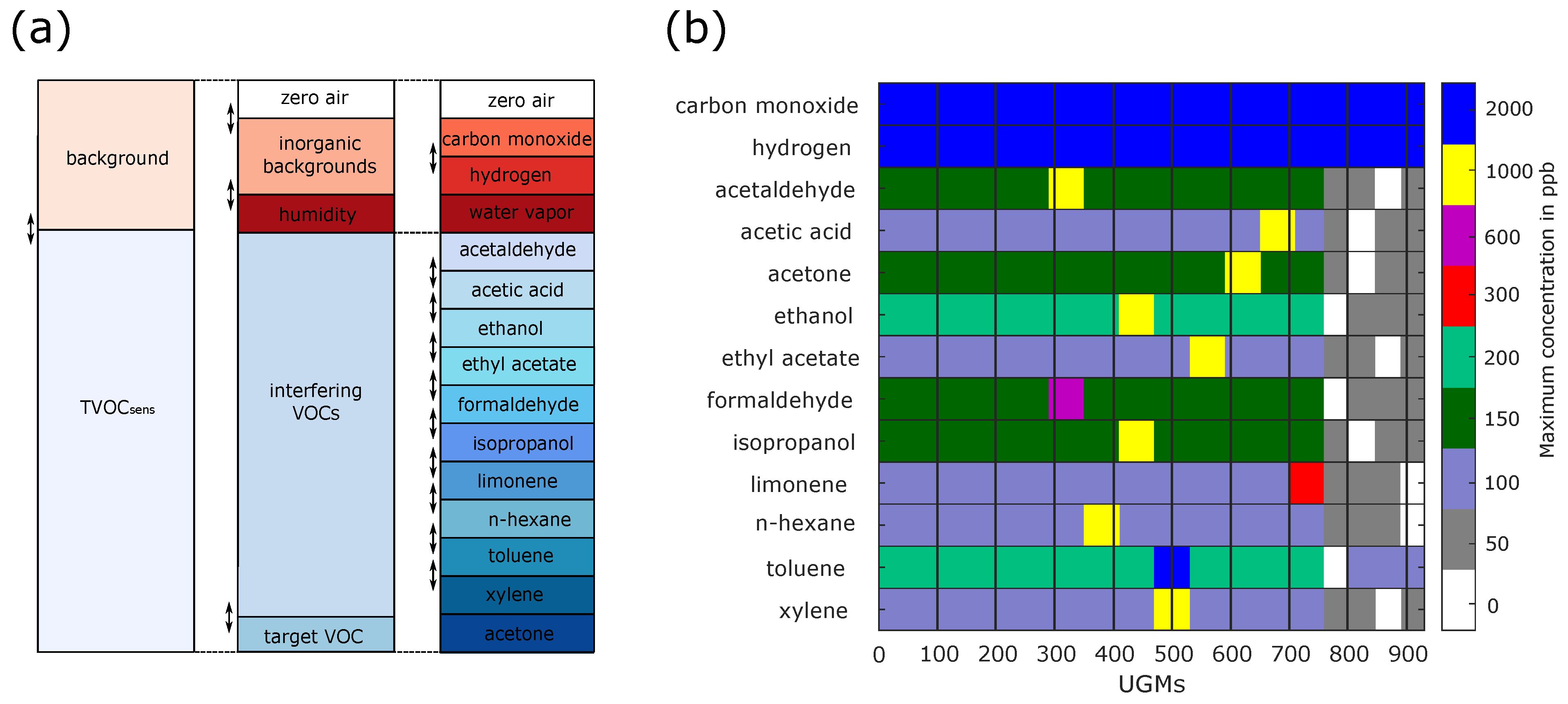
The dataset used throughout this study was recorded with a custom gas mixing apparatus (GMA) [34,35,36]. The GMA allows us to offer precisely known gas mixtures to multiple sensors simultaneously. The latest version of the GMA can generate gas mixtures consisting of up to 14 different gases while also varying the relative humidity [37]. A specific gas mixture of predefined gas concentrations and relative humidity is called a unique gas mixture (UGM). Within this work, a unique gas mixture consists of zero air, two background gases (carbon monoxide, hydrogen), relative humidity, and eleven different VOCs, as illustrated in Figure 1. Since many different UGMs are required to build a regression model for a gas sensor, multiple UGMs are necessary. This dataset consists of 930 UGMs, randomly generated with the help of Latin hypercube sampling [38,39]. Latin hypercube sampling implies that each gas concentration and the relative humidity is sampled from a predefined distribution (in this case, uniformly distributed) such that the correlation between the independent targets is minimized. This prevents the model from predicting one target based on two or more others. This method has been proven functional in previous studies [39]. However, this process is extended with extended and reduced concentration ranges at low (0–50 ppb) and very high (e.g., 1000 ppb) concentrations. All concentration ranges can be found in Figure 1b. The range for the relative humidity spanned from 25% to 75%. A new Latin hypercube sampling was performed every time a specific range was adjusted. Moreover, because only one observation per UGM is not statistically significant, ten observations per UGM are recorded. However, the GMA has a time constant and the new UGMs could not be applied immediately, so five observations had to be discarded. Nevertheless, this resulted in 4650 observations for the calibration dataset.

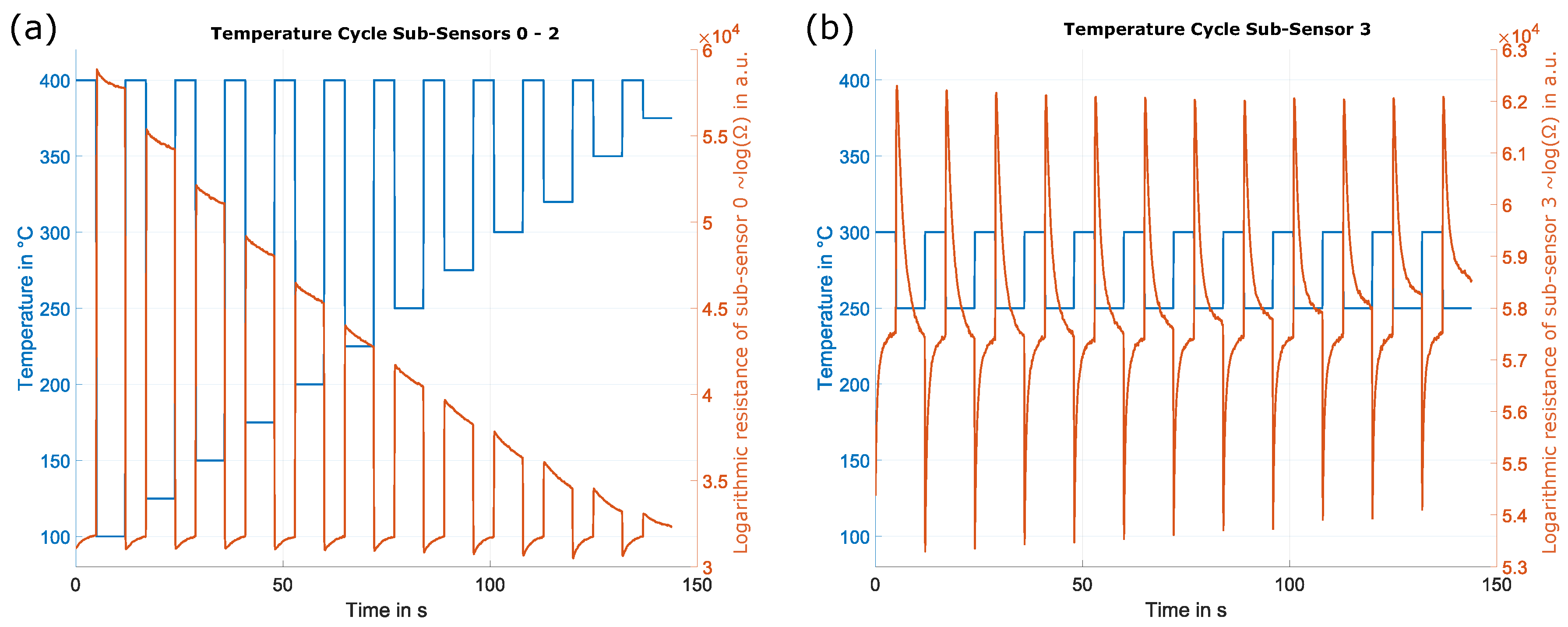
After discussing the UGMs applied to the different gas sensors, the next important part of the dataset is the sensor used and how the sensor is operated. The sensors used within this dataset are SGP40 sensors from Sensirion (Sensirion AG, Stäfa, Switzerland). Those sensors have four different gas-sensitive layers on four individual micro-hotplates. A non-disclosure agreement made it possible to operate the sensors in temperature cycled operation (TCO) [40]. Temperature cycled operation means that with the help of the micro-hotplates of the sensor, the independent gas-sensitive layers can be heated in specific temperature patterns during operation. One temperature cycle for sub-sensors 0–2 (gas-sensitive layer) consists of 24 phases. First, the sub-sensor is heated to 400 ${}^{\circ }$C for 5 s, followed by a low-temperature phase at 100 ${}^{\circ }$C for 7 s. This pattern is repeated twelve times in one full temperature cycle with increasing low-temperature phases (an increase of 25 ${}^{\circ }$C per step). This leads to twelve high- and low-temperature steps, as illustrated in Figure 2. The temperature cycled operation for sub-sensor 3 is slightly different; here, the temperature cycle repeats the same high and low-temperature levels. The high temperature is always set to 300 ${}^{\circ }$C, and the low temperature to 250 ${}^{\circ }$C (cf. Figure 2). As described earlier, a temperature cycled operation was used to increase the selectivity of the different sensors. Therefore, the whole temperature cycle takes 144 s, resulting in 1440 samples (sample rate set to 10 Hz). The sensor response during one temperature cycled operation results in a matrix of $4\times 1440$ and represents one observation. In total, the response of seven SGP40 sensors (S1–S7) for all UGMs is available for this study.

2.2. Model Building

In the first step, the calibration dataset is divided into 70% training, 10% validation, and 20% testing. A crucial point regarding the data split is that the splits are based on the UGMs rather than observations. In order to make the fairest comparison possible, this split is static across all different model-building methods and sensors throughout this study, which means that for every evaluation, the same UGMs are in either training, validation, or test set.

After the data split, two different methods for model-building are introduced. One model-building approach is feature extraction, selection, and regression (FESR), which was intensively studied earlier [13,40,41]. The other method, TCOCNN, was developed recently in [29,42] and has already proven to challenge the classic methods.

2.2.1. Feature Extraction, Selection, and Regression

The first machine learning approach introduced is feature extraction, selection, and regression (FESR). This method first extracts sub-sensor-wise features from the raw signal, selects the most important ones based on a metric, and then builds a regression model to predict the target gas concentration. The algorithm can learn the dependencies between raw input and target gas concentration during training. If multiple SGP40 sensors are used for training, the input size of the model does not change. Instead, the model only gets more observations to learn.

This study uses the adaptive linear approximation as a feature extraction method [43]. Although the algorithm can identify the optimal number of splits, this time, the algorithm is forced to make exactly 49 splits for each sub-sensor independently, which ensures that every temperature step can be accurately reconstructed. The position of the optimal 49 splits is determined by the reconstruction error, as described in [44], cf. Figure 3. The mean and slopes are calculated on each resulting segment. Since there are four sub-sensors and 50 segments each, this results in 400 features per observation.

Afterward, features are selected based on their Pearson correlation to the target gas to reduce the number of features to the most essential 200. After that, a partial least squares regression (PLSR) [45] with a maximal number of 100 components was trained on 1–200 Pearson-selected features in a 10-fold cross-validation based on training and validation data to identify the best feature set. Finally, another PLSR was trained with the best feature set on training and validation data to build the final model. This combination of methods achieves reasonable results, as reported earlier [46].

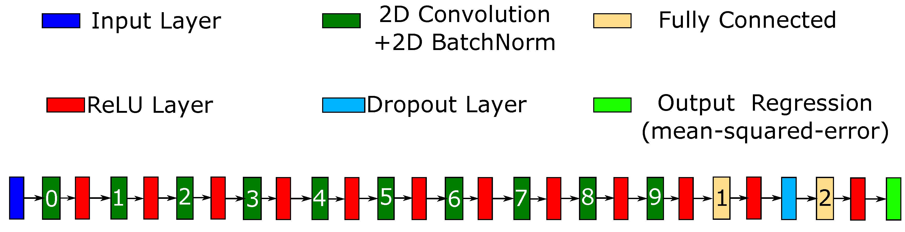
2.2.2. Deep Learning: TCOCNN

The TCOCNN is a convolutional neural network [42,47] specifically tailored for MOS gas sensors operated in temperature cycled operation. Figure 4 gives an example of the network. The TCOCNN takes as an input a $4\times 1440$ matrix. Four represents the number of sub-sensors per gas sensor, and 1440 is the number of sample points in the temperature cycles.

The network consists of multiple hyperparameters that can be tuned with the help of the training data, the validation data, and a neural architecture search. The hyperparameters adjusted within this study are the kernel width (10–100) of the first two convolutional layers, the striding size (10–100) of the first two convolutional layers, the number of filters in the first layer (80–150), the depth of the neural network (4–10; including the last two fully connected layers), the dropout rate during training (10–50%), the number of neurons in the fully connected layer (500–2500), and the initial learning rate. A more detailed explanation of the neural architecture search based on Bayesian optimization can be found in [42,49,50]. In order to optimize the hyperparameter, the default setup for the Bayesian optimization of Matlab is used for 50 trials. The optimization of the validation error is conducted only once with sensor 1. Afterward, the same parameters are used throughout the study, and all further tests are performed on the test data, which prevents the results from overfitting. The parameters found for this study are listed in

Table 1. Values of all hyperparameters. The number of filters, striding size, and kernel size concern the first two layers, the number of neurons concerns the second to last fully connected layer, and the number of layers includes the convolutional layer and the last two fully connected layers.

Filters	Striding Size	Kernel Size	Layer	Number of Neurons	Initial Learning Rate	Dropout Rate
83	34	63	8	1312	$4.3·{10}^{-4}$	13.83%

. The derived parameters are given as follows: the number of filters is doubled every second convolutional layer; the striding size after the first two convolutional layers follows the pattern $1\times 2$ then $1\times 1$, and the same is applied for the kernel size; and finally, the initial learning rate decays after every second epoch by a factor of 0.9.

2.3. Calibration Transfer

Because of manufacturing tolerances, the responses of two sensors (same model) will always show different responses [51]. Therefore, calibration of every sensor is necessary to predict the target gas concentration. In our case, this calibration was carried out with the data recorded under laboratory conditions. However, many calibration samples are necessary before a suitable calibration is reached. Therefore, the idea is to reuse the calibration models of different sensors instead of building a new one every time (calibration transfer) [22,52,53]. The goal is to significantly reduce the number of samples needed for calibration.

The calibration transfer is usually performed based on a few transfer UGMs. In order to make the comparison as fair as possible, the transfer samples are always the same for every evaluation. However, they are chosen randomly (but static) from all available training and validation UGMs.

2.3.1. Signal Correction Algorithms

As described above, the goal is to use the same model for different sensors to reduce calibration time. However, because the differences between sensors are usually too significant, it is impossible to use the same model immediately. One common approach is to match the signal of the new sensor to the sensors seen during training [21,25,27]. The sensor (or sensors) used for building the initial model is called the master sensor, and the new sensor, which is adapted to resemble the master sensor (or sensors), is called the slave. In the matching process, the signal of the slave sensor is corrected to resemble the signal of the master. This is usually done by taking multiple samples (transfer samples) where the master and slave sensors are under the exact same conditions and then calculating a correction matrix (C) that can be used to transform the slave signal to match that of the master also under different conditions.

Direct standardization is one of the most common methods used for calibration transfer in gas sensor applications [21,25,27]. The correction matrix is calculated for direct standardization, as shown in Equation (1) [25,54,55].

$$C=R_S^{+}·R_M$$

(1)

Here, C represents the correction Matrix, $R_S^{+}$ stands for the pseudoinverse of the response matrix of the slave sensor, and $R_M$ resembles the response matrix of the master sensor. The response matrices are of the shape ${\mathbb{R}}^{n\times m}$, and n resembles the number of samples needed to apply for calibration transfer (e.g., 25 observations or 5 UGMs), and m stands for the length of one observation, e.g., 1440 for one sub-sensor. Therefore, the resulting Matrix C is of the size ${\mathbb{R}}^{m\times m}$ and is applied to new samples as given in Equation (2).

$$R_{S;C}=C·R_S$$

(2)

Since the SGP40 consists of multiple sub-sensors, this approach is used for each sub-sensor independently. However, suppose various sensors (multiple SGP40) are used as the master sensors for signal correction. In that case, the slave responses are repeatedly stacked, and the different master sensors (all under the same condition) are stacked into one tall matrix.

As an example, the responses of two master sensors and one slave sensor under the same condition led to the correction matrix given in Equation (3).

$$C={\left[\begin{array}{c}{R}_S\\ R_S\end{array}\right]}^{+}·\left[\begin{array}{c}{R}_{M1}\\ R_{M2}\end{array}\right]$$

(3)

The drawback of this method is that the construction of C requires the pseudoinverse of the response matrix, and the number of available transfer samples determines the quality. Since this study aims to reduce the number of transfer samples as much as possible, another signal correction algorithm is introduced. Piecewise direct standardization [55] uses the same approach as direct standardization, but the C parameter is calculated for small subsections of the raw signal. This means that before piecewise direct standardization (PDS) is applied, the signal is divided into z segments of length p.

Therefore, C can be calculated as shown in Equation (4) on small segments of length p.

$$C_P=R_{S;p\times n}^{+}·R_{M;n\times p}$$

(4)

$C_P$ has the shape ${\mathbb{R}}^{p\times p}$, and the final C matrix is calculated by assembling those smaller Cs (total z different Cs) on the diagonal. This means that C for a small segment of length p is calculated based on Equation (5).

$$C=\left[\begin{array}{cccc}{C}_{P1}& 0& \cdots & 0\\ 0& \ddots & & ⋮\\ ⋮& & & 0\\ 0& \cdots & 0& C_{Pz}\end{array}\right]$$

(5)

The final C is again of the shape ${\mathbb{R}}^{m\times m}$ and can be used as before. However, this leads to the conclusion that piecewise direct standardization has one hyperparameter that can be tuned. For this study, p is chosen to be 10. This was defined by testing a calibration model with one master and one slave sensor on multiple different window sizes (also two windows of different possible sizes) and choosing the window size with the smaller RMSE, as listed in

Table 2. RMSE values for different window sizes for the piecewise direct standardization. Piecewise direct standardization was performed with five transfer samples. The RMSE was achieved by training the model with data from one master sensor, and testing was performed on the adapted data of the slave sensor. Entry 50;70 represents alternating window sizes to precisely cover the TCO shape.

Window width	5	10	20	50;70
RMSE in ppb TCOCNN	28.3	26.3	43.8	59.1
RMSE in ppb FESR	47.9	55.4	123.6	209.0

.

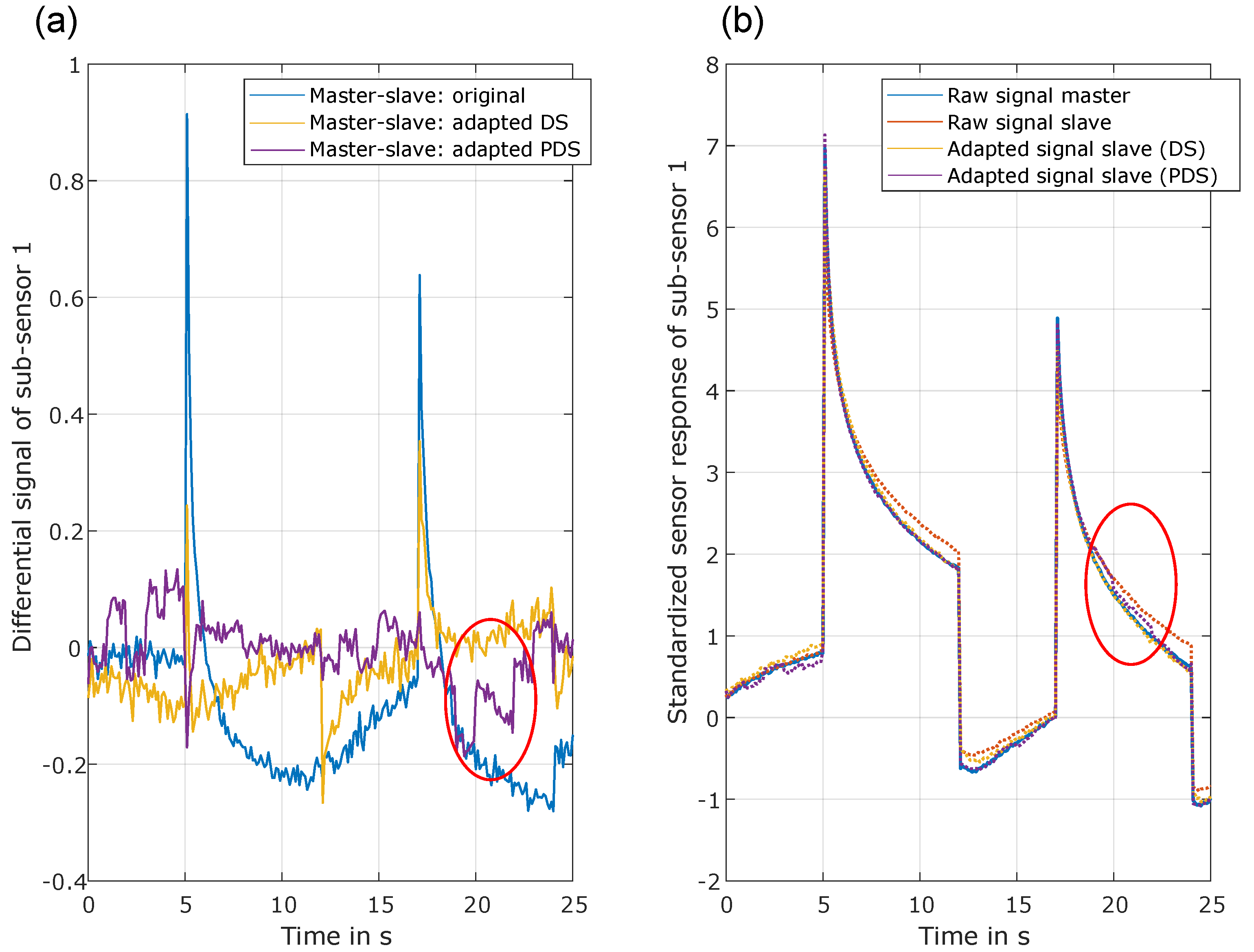
Although piecewise direct standardization is expected to achieve better results [25] as the calculation of C is more robust than direct standardization, both approaches are analyzed in this study. This is reasonable, as indicated by Figure 5, which illustrates the original signal of the master and slave sensor, together with the adapted (corrected) signal and the differential signal. Although the purple line (corrected signal PDS) follows the master signal more precisely, it is possible to spot small jumps that might influence the prediction quality. This is not visible for direct standardization, but in this case, the corrected signal is further apart from the master signal, especially when analyzing the peaks in the differential signal.

A significant benefit of signal correction methods is that they are independent of the used model and can be applied to the FESR approach and the TCOCNN.

2.3.2. Transfer Learning for Deep Learning

Compared to the signal correction methods, the transfer learning method for deep learning can only be applied to the TCOCNN. This method adjusts the whole model to the new sensor instead of correcting the raw signal of the new (slave) sensor. Transfer learning is a common approach in deep learning, especially in computer vision [31,32,33]. Multiple works have shown that this approach can significantly reduce errors and speed up training [33,56]. In previous studies, it was demonstrated that transfer learning could also be used to transfer a model trained on gas sensor data based on many calibration samples to a different sensor with relatively few transfer samples [28,29,53] (calibration sample reduction by up to 97% (700 UGMs–20 UGMs). An essential extension to previous studies is that the initial model is built with the help of multiple sensors, which should increase the performance even more.

The idea is illustrated in Figure 6. While the blue line resembles a model trained from scratch, the other two show the expected benefit when adjusting (retraining) an already working model to a new sensor. The modified model needs much fewer UGMs to get to a relatively low RMSE, and the improvement is much steeper. The hyperparameter to tune transfer learning is typically the learning rate. All hyperparameters of the TCOCNN are the same as before, and only the initial learning rate is set to the learning rate typically reached halfway through the training process. Of course, it would also be possible to tune this process with the help of Bayesian optimization to achieve even better results. However, this was not tested in this study, and the optimal value obtained in other studies is used [29].

A significant benefit compared to signal correction methods is that for this approach, the transfer can happen even if the sensors were never under the same condition, which makes even a transfer between datasets possible.

2.4. Evaluation

After introducing the general methods used throughout this study, this section introduces the techniques to benchmark the different methods.

The first part will evaluate the performance of the FESR and TCOCNN approach regarding their ability to predict the target gas concentration. This will be done by using multiple sensors to build the models. The training and validation data of one to six sensors will be used to train six FESR and six TCOCNN models (increasing the number of sensors). Afterward, the models will be tested on the corresponding sensors’ test data. This will then be used as a baseline for all further evaluations.

In the next step, the performance of a model trained with each of the available six sensors (trained independently) is tested with the test data of sensor 7. This is done to test the generalizability of a model trained with one sensor and tested with another sensor. Afterward, the models are trained on one to six sensors (same as baseline models), and after that, the generalizability is tested with the test data of sensor 7.

The last part then focuses on methods to improve generalizability. Therefore, multiple methods from the field of calibration transfer will be used. The initial models are again built with the training and validation data of sensors 1–6. This results in twelve initial models, which are used to test transfer learning, direct standardization, and piecewise direct standardization (six FESR models, and six TCOCNNs). After the initial models are built, transfer learning and the signal correction algorithms are applied as explained above with 5, 25, 100, and 600 transfer UGMs. In order to have a more sophisticated comparison, a global model is also trained on 1-6 sensors plus the transfer samples. This means the transfer data are already available during initial training to determine if that also improves the generalizability. Those results then allow a general comparison of the most promising methods.

For comparing the different methods, the root mean squared error (RMSE) is used as the metric to rate the performance of the various models. Also, other methods like R-squared, mean absolute error (MAE), or mean absolute percentage error (MAPE) can been used. However, the main goal in indoor air quality monitoring is to know if a certain threshold is exceeded and how far the estimation can be off the target value to account for a margin. Therefore, the RMSE as an interpretable metric is used. Furthermore, this study should mainly focus on the prediction quality’s general trend rather than analyzing every aspect of the regression model. At the beginning of the results section, a scatter plot illustrating the target vs. the predicted value is shown, and the r-squared values are given to prove that the models work as intended.

As a final remark, the evaluations with the TCOCNN are repeated five times to consider the model’s uncertainty.

3. Results

As described above, the first step is to create a baseline to interpret the following results. Figure 7 shows the results when training the initial model with 1–6 sensors (744 UGMs per sensor). For any number of sensors, the TCOCNN outperforms FESR. With an increasing number of sensors used to build the model, the RMSE value decreases for the TCONN, while it increases for FESR. This means the model can generalize and find a better model with more data from multiple sensors. The reason for the TCOCNN outperforming the FESR approach might be the more advanced feature extraction compared to the static extraction of the FESR. In order to give the RMSE values more context, the prediction on the test data for the FESR and TCOCNN models are shown in Figure 7b. There, it can be seen that despite the worse RMSE, the FESR approach still shows a suitable relationship between target and prediction (r-squared > 0.96). However, it must be mentioned that at high concentrations, the accuracy worsens for both models. This is because this region has fewer data points (extended concentration range). Nevertheless, this is not a problem since the threshold for the target gases is usually at smaller concentrations (more data points). It is essential to be very precise in lower regions, and beyond that point, it is sufficient to identify that the threshold is exceeded. Therefore, an RMSE of around 25 ppb can still be interpreted as a suitable model since the error is in an acceptable range, and the correlation is always (also for the upcoming results) clearly visible, like in Figure 7b (r-squared > 0.96).

After analyzing the performance of the initial model on the test data of the corresponding sensors, the next step is to test the initial model on the test data of a completely different sensor. The first evaluation is carried out by training an independent model with one sensor each and testing the performance on the test data of sensor 7. The results are depicted in Figure 8a. It can be seen that it strongly depends on the sensor if the TCOCNN or FESR approach can find a general model to apply to multiple sensors. For example, the TCOCNN for sensor 6 achieves good results with sensor 7, while the model for sensor 1 applied to sensor 7 does not work. As seen by sensor 3, this also depends on the evaluation method. For example, sensors 3 and 7 are deemed similar by the FESR approach, while the TCOCNN indicates differently. This might be because both ways rely on different features. While the TCOCNN generates features independently, the FESR approach has fixed features based on the adaptive linear approximation. Since the scope of this article is not to highlight the different features used within the various methods, this will not be discussed in more detail. However, it was already shown in [51] that different methods are available (e.g., occlusion map) to identify the different feature sets used by the methods, depending on the sensor. Nevertheless, this does not mean that a model that is useful for multiple sensors can be applied to all SPG40 sensors—only to those similar. Therefore, Figure 8b illustrates the results that can be achieved with the initial models when trained with 1-6 sensors simultaneously. It can be seen that with increasing sensors, the TCOCNN model generalizes more and can be applied more successfully to sensor 7. However, the improvement does not directly correlate with the independent performance (Figure 8), which might be because the model needs to generalize more to suit all sensors, which then generalizes too much and causes the performance to drop (e.g., the TCOCNN with sensor 5).

However, the model trained with six sensors achieves an RMSE of 31 ppb, close to the suitable RMSE of 25 ppb from the baseline of the FESR method. In comparison, the TCOCNN achieves almost acceptable results without calibration transfer, while the FESR approach trained with multiple sensors struggles. Though the RMSE also generally shrinks in the case of sensor 7 when more sensors are used for training with the FESR approach, the results are worse than those of the TCOCNN. This can have multiple reasons. One reason could be that the approach of adaptive linear approximation, Pearson selection, and PLSR are not optimal for this task. A more sophisticated FESR approach based on a more sophisticated feature extraction and recursive feature elimination least squares as a feature selection might yield more promising results. However, because of the limited performance of the FESR approach for this specific setup in the baseline and the initial model building, the remaining results will only cover the results achieved with the TCOCNN. The results of the FESR approach are listed in Appendix A.

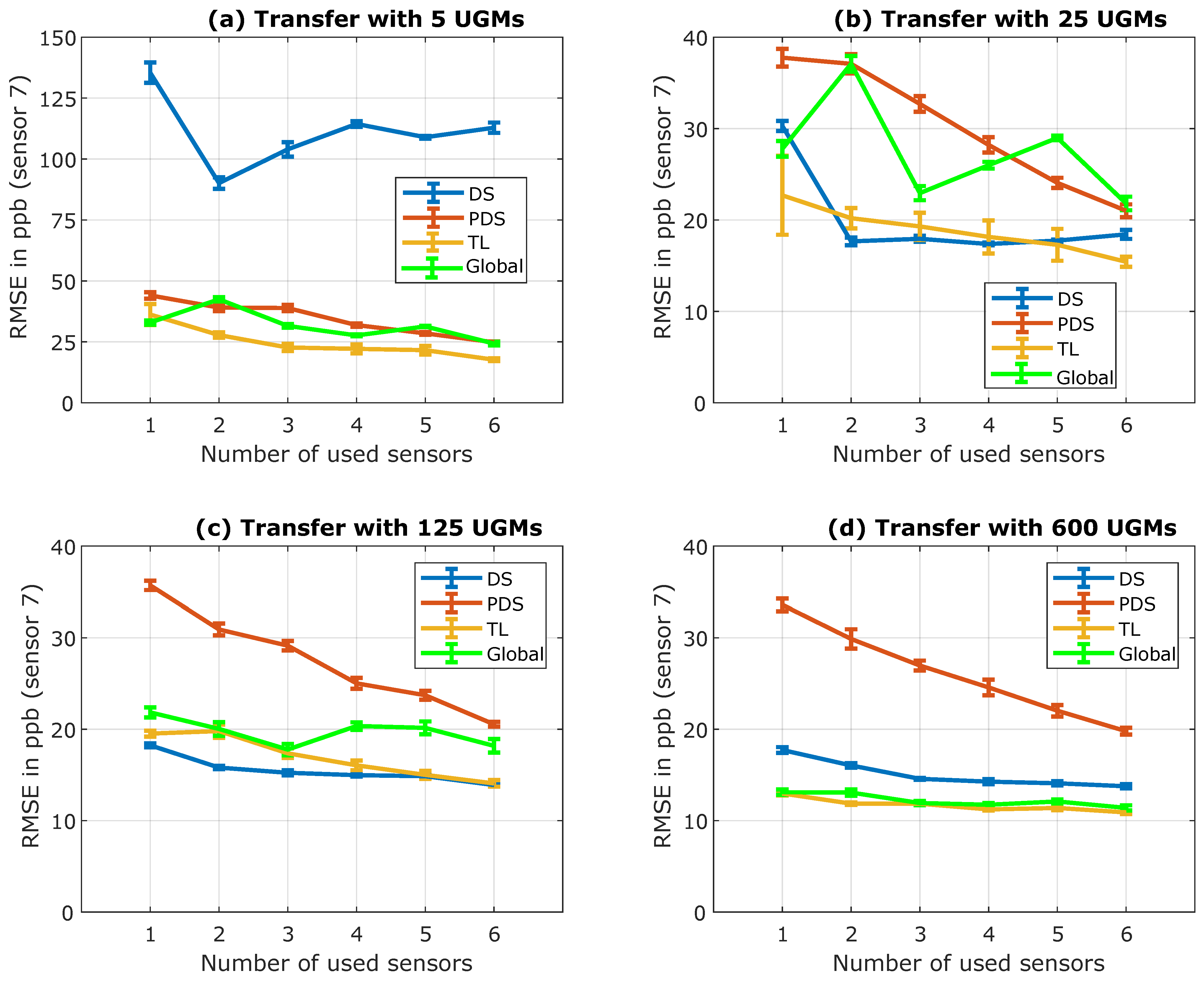
After discussing the capability of the different machine learning methods to generalize across sensors, the next step is to evaluate the signal correction methods, transfer learning, and global model building (all available data used for training). Figure 9 depicts the results achieved with different initial models (built with 1–6 sensors) on the x-axis of each sub-figure, and it also shows the effect of the different number of transfer UGMs. In Figure 9a (five transfer UGMs), it can be seen that direct standardization does not achieve any reasonable results, which might be correlated with the problem of not having enough transfer samples to invert the matrix. As expected, the piecewise direct standardization performs much better as, from theory, the pseudoinverse should be much more manageable to calculate. However, the best method, in this case, is the transfer learning approach. While this approach does not perform exceptionally well if only one sensor is used to build the initial model, with six sensors for the initial model building, an RMSE of 17.7 ppb can be achieved, which is better than the FESR baseline cf. Figure 9. That would mean a suitable model was created with only 5 UGMs (instead of 744). The reason that transfer learning can outperform the other method might be because of the advanced feature extraction that generalizes well across sensors and because only small adjustments inside the model are necessary. Similar but less impressive results can be observed for global model building and piecewise direct standardization (six sensors for the initial model); there, a reasonable RMSE of 24.3 ppb was achieved (again, smaller than the baseline FESR). The slightly worse performance compared to transfer learning can be attributed to the nonspecific model. While transfer learning generates a specific model for the new sensor, the global approach tries to find a model to fit all. Figure 9b (25 UGMs for transfer) indicates that if enough transfer samples are available, direct standardization can perform much better than piecewise direct standardization and achieves results similar to transfer learning. This might be because the pseudo inverse can now be calculated appropriately. However, with six sensors for the initial model, each method achieves an RMSE below 25 ppb, which is again better than the FESR approach’s baseline, which indicates that all methods are suitable. Nevertheless, the best performance is again shown by transfer learning.

The two sub-figures at the bottom show the benefit of more transfer samples. Figure 9c (125 transfer samples) indicates that direct standardization and transfer learning perform similarly for this case, and that piecewise direct standardization does not improve significantly. Furthermore, global modeling and transfer learning has become ever so close. Moreover, it can be derived that the amount of transfer samples is now always sufficient for the pseudo inverse of direct standardization. While 25 UGMs with one sensor is almost insufficient, the improvement between one and two sensors for 125 UGMs is much smaller. Figure 9d then concentrates on the results if 600 transfer samples (almost all training samples) are used. Global modeling and transfer learning perform more or less similar and now even achieve results smaller than the baseline of the TCOCNN from earlier, which was 12.1 ppb. This aligns with the baseline results of the TCOCNN as the RMSE also dropped by adding more sensors. Furthermore, more transfer samples do not improve the direct standardization and piecewise direct standardization results. This might be because it does not help to make the slave sensor more similar to the master sensors anymore (as already seen for 125 UGMs).

Since the sensor manufacturers are most interested in significantly reducing calibration time, the most suitable method seems to be transfer learning, as this method achieves a reduction in calibration UGMS of 99.3%. For small transfer sets, piecewise direct standardization and global model building also achieve good results. However, it has to be noted that global model building outperforms transfer learning and piecewise direct standardization regarding small initial datasets.

To emphasize the benefit of transfer learning compared to global modeling, Figure 10 illustrates the side-by-side comparison of both approaches over the different number of transfer UGMs regarding an initial model built with one sensor, and one where the initial model was constructed with all six sensors. The most important part is in relation to the five transfer UGMs. While the benefit of transfer learning compared to global model building is not apparent when the initial model is built with only one sensor, the effect can be seen when six sensors are used. Figure 10b indicates that transfer learning shows its full potential when trained with more sensors. While global model building achieves an RMSE of only 24.9 ppb, transfer learning can get as low as 17.7 ppb. This is in accordance with the theory that a model trained simultaneously with the initial and transfer data cannot adapt to the new sensor like the specifically tailored model obtained by transfer learning.

After showing that transfer learning is a very promising method to reduce the calibration time significantly, it can be seen in Appendix A that for the FESR approach, the same phenomena as explained above can be observed. However, the results of the FESR approach are not as good as those of the TCOCNN since the baseline is worse. Furthermore, it seems that the FESR approach does not work well with piecewise direct standardization, possibly because of the small edges in the adapted signal.

4. Discussion

After analyzing the baseline results and the calibration transfer methods, the TCOCNN shows the most promising result when it comes to generalizability. Furthermore, it was shown that, especially with the TCOCNN, using multiple sensors for the initial model building could be beneficial. Even without calibration transfer methods, applying a model trained with six sensors to a new sensor was possible, and suitable results of around 32 ppb were achieved. This can be attributed to the more flexible feature extraction of the TCOCNN, which allows for better generalizability. Furthermore, different sensors’ effects on the initial model building were investigated. Here, it was shown that it makes a significant difference which sensors are used to build the initial model. It was shown that when only one sensor is used for model building, the results can differ by up to 45 ppb concerning the new sensor (for difference in the sensor response, see [51]). This might be interesting to investigate in future experiments. Nevertheless, it was shown that the most effective way to achieve the lowest RMSE values possible is to use calibration transfer. Transfer learning proved to be the best option since this method outperformed every other approach when the initial model was trained with many sensors and only a few transfer samples were available. It was shown that with less than 99.3% of the calibration UGMs, results of 18 ppb are still possible (better than the FESR baseline). Compared to the other methods, the exceptional performance can be attributed to the specifically retrained network. However, the other methods showed decent results as well. As expected, piecewise direct standardization performs well for minimal transfer sets and can even outperform direct standardization since the calculation of the pseudo-inverse is more straightforward. Direct standardization showed the full potential if 25 transfer UGMs were available (manageable pseudo inverse) and surpassed transfer learning if smaller initial datasets were investigated. Global model building performed very similarly, although transfer learning outperformed global model building significantly when large initial and small transfer datasets were concerned. This might be because a more general model is appropriate for this task. Moreover, the calibration methods for signal correction and global model building also worked for the FESR approach, although further improvements need to be made to be compatible with transfer learning.

5. Conclusions

This study’s results allows the conclusion that transfer learning is a powerful method to reduce the calibration time by up to 99.3%. It was shown that transfer learning could outperform the other techniques, especially with small transfer sets and initial models trained on multiple sensors. Furthermore, it was shown that the other calibration transfer methods are comparable, especially for the most important case of 5 transfer UGMs. Piecewise direct standardization or global model building with many sensors for initial model building also achieved decent results with 5 UGMs for transfer (24.3 ppb). In comparison, direct standardization needed at least 25 transfer UGMs. The FESR approach did not show optimal results, but this might be possible if a method combination is found that is more tailored to calibration transfer. This would be beneficial because the computational effort would be much smaller.

For further research, it would be exciting to see how the TCOCNN performs in combination with (piecewise) direct standardization and transfer learning. Furthermore, it was not investigated if something similar is possible if two different datasets with different gases (same target gas) are used. One interesting extension of this work is to analyze how the models differ (explainable AI) when using multiple sensors and whether it is possible to generate FESR methods based on insights gained with techniques from explainable AI. It is also possible to build an error model based on multiple sensors’ raw signals to apply data augmentation and further improve the results. It should also be determined in future work if transfer learning can be used to compensate for drift. Furthermore, this study only covers the specific case of indoor air quality monitoring. Future research should also extend this approach to breath analysis, outdoor air quality monitoring, and other sensor calibration tasks.