Article

Projection and Analysis of Floods in the Upper Heihe River Basin under Climate Change

1
School of Water Resources and Environment, China University of Geosciences (Beijing), Beijing 100083, China
2
MOE Key Laboratory of Groundwater Circulation and Environmental Evolution, Beijing 100083, China
3
State Key Laboratory of Hydrology-Water Resources and Hydraulic Engineering, Nanjing Hydraulic Research Institute, Nanjing 210029, China
4
College of Water Sciences, Beijing Normal University, Beijing 100875, China
*
Author to whom correspondence should be addressed.
Atmosphere 2023, 14(7), 1083; https://doi.org/10.3390/atmos14071083
Submission received: 8 June 2023 / Revised: 24 June 2023 / Accepted: 26 June 2023 / Published: 28 June 2023
(This article belongs to the Section Climatology)

Abstract

:
The projection of future hydrological processes can provide insights into the risks associated with potential hydrological events in a changing environment and help develop strategies to cope with and prevent them. The Heihe River basin in Northwest China is crucial for providing water resources to water-scarce regions. Thus, understanding the future runoff trends in the context of climate change can optimize water allocation, alleviate water shortages, and mitigate flood risks in the region. In this study, we use meteorological data from 10 general circulation models under two future scenarios to drive the Soil and Water Assessment Tool (SWAT) model and project hydrological processes in the upper Heihe River basin from 2026 to 2100. After examining the future changes in total runoff in the basin, we assess the magnitude, frequency, and timing of daily flood events in the future. The results of the multi-model ensemble averaging (MMEA) method show that the change in the multi-year average annual runoff is −4.5% (2026–2050), −1.8% (2051–2075), and +2.0% (2076–2100) under the SSP245 scenario and −1.0% (2026–2050), +0.4% (2051–2075), and +0.2% (2076–2100) under the SSP585 scenario compared to the historical period. The analysis of flood magnitudes indicates that the basin will experience higher-magnitude floods in the future, with the largest increase rates of 61.9% and 66.4% for the 1-day maximum flows under the SSP245 and SSP585 scenarios, respectively. The flood return period is projected to be shorter in the future, and the 1-day maximum flows of a 100-year flood are expected to increase by 44.7% and 63.7% under the SSP245 and SSP585 scenarios, respectively. Furthermore, a significant shift in the flood timing is expected, with the highest frequency moving from July to August, representing a one-month lag compared to the historical period. Our findings suggest that the hydrological characteristics of the upper Heihe River basin may be significantly altered in the future due to the effects of climate change, resulting in floods with higher magnitudes and frequencies and different timings. Therefore, it is imperative to consider these changes carefully when developing risk prevention measures.

1. Introduction

Extreme hydrological events can result in significant social and property losses, including damage to homes, businesses, and infrastructure, as well as threats to human lives and livelihoods [1,2,3]. According to the Intergovernmental Panel on Climate Change (IPCC) Sixth Assessment Report (AR6) of April 2022, global greenhouse gas emissions have reached record levels in the last decade, and substantial future warming is inevitable [4]. This will result in considerable uncertainty and changes in precipitation, temperature, wind speed, air pressure, and other meteorological factors, affecting the timing, frequency, and intensity of hydrological events [5,6,7,8,9]. The impacts of climate change may include more frequent and severe droughts and floods and other associated risks [10,11,12,13,14,15].
Numerous studies have shown that the occurrence of floods is strongly influenced by a range of factors, including the amount of water vapor in the atmosphere, rainfall intensity and duration, the geographical and temporal patterns of precipitation, and subsurface conditions, such as soil type and topography [16,17,18]. Climate change may alter the characteristics of flood hazards since the physical elements contributing to floods, such as atmospheric moisture, precipitation, and subsurface conditions, may also change substantially under climate change [8,16,19,20,21,22]. It is crucial to reassess our understanding of flood risk and develop more resilient flood control and mitigation strategies to mitigate these risks and protect the environment.
Studies have shown that climate change will cause large uncertainties in the projection of future hydrological conditions, and this part of the uncertainty will also be transferred to future hydrological processes in the process of coupling climate change projection with hydrological models [23,24,25,26,27,28]. Therefore, researchers often use multiple climate models based on multiple scenarios to provide a range of possible outcomes. Additionally, changes in climate-related physical elements may alter different aspects of hydrological processes, requiring distributed models based on physical significance to estimate future hydrological processes more accurately [29,30,31]. By using these models, researchers can better understand the complex interactions between climate change and the hydrological cycle and develop more effective management strategies to address potential future risks.
Eingrüber et al. [18] used the general circulation model (GCM) HadCM3 to drive the Soil and Water Assessment Tool (SWAT) and found that flood events in the Ruhr basin, Germany, would become more frequent and intense due to changes in atmospheric circulation, resulting in a significant shortening of the flood return period. Iqbal et al. [22] used four GCMs from the Fifth Coupled Model Intercomparison Project (CMIP5) and the SWAT model to study flood intensity and frequency in the Kabul Basin. They found that the melting rate of snow and glaciers in the region would accelerate in the future due to increased precipitation and temperature, leading to increased flooding. The latest CMIP6 considers a broader range of socioeconomic pathways and provides more diverse emission scenarios than the CMIP5 [32,33,34], improving the relevance to real-world conditions. Yang et al. [20] used GCMs from the CMIP6 to assess the future hydrological processes in the Jiulong River basin. They found that climate change was the dominant cause of future high-flow increases, with expected increases in the average future 100-year flood frequency exceeding 100% and 200% under the SSP126 and SSP370 scenarios, respectively. Xiang et al. [21] evaluated the future hydrological conditions of the Yarkant River basin based on six GCMs from the CMIP6 and three shared socioeconomic pathways. The results suggested that the future hydrological conditions in the region were likely to change significantly, with more frequent extreme hydrological events.
The Heihe River basin is located in a dry and arid region of Northwest China and is primarily fed by precipitation and glacial meltwater from the Qilian mountains [19,35,36,37,38]. In recent years, the increase in water demand for livestock, agriculture, domestic water, etc., has made the ecosystem of the basin more fragile [39,40]. Therefore, it is necessary to study the long-term water resource quantity changes in this basin. Zhang et al. [41] used various statistical methods to explore changes in historical runoff trends in the Heihe River basin and found that increased precipitation and rising temperatures were responsible for the increase in upstream runoff. Luo et al. [42] explored the drivers of surface runoff changes in the upper Heihe River basin based on the SWAT model and pointed out that runoff changes in spring and winter are mainly influenced by temperature, while summer runoff is influenced by precipitation. Shang et al. [43], when studying the impact of land use and climate change on surface runoff change, pointed out that the impact of climate change is far greater than that of land use, and the change in precipitation is stronger than that for temperature. Projections of future runoff are also of great significance in the context of the current changing climate. Li et al. [35] used three GCMs to project future runoff changes in the upper Heihe River basin under the representative concentration pathway (RCP) 4.5 scenario and found that more runoff would occur due to increased precipitation. Zhang et al. [36] used the SWAT model to simulate future hydrological processes in the upper Heihe River basin from 2021 to 2050 and found that the runoff was expected to increase by 11.4% and 12.8% under the RCP4.5 and RCP8.5, respectively. Many studies have focused on the total runoff changes under climate change [35,36,37,38].
Although extreme hydrological events are worth studying because they cause severe social and economic losses, there is little research on these events in the Heihe River basin. According to statistics, there have been 71 floods in the basin in the past 2000 years, and the number of floods has been on the rise since the 18th century. With the intensification of global warming, the impact of floods in the late 20th century far exceeded that of other decades, with the frequency of occurrence reaching an average of 1.8 times per decade [44,45,46]. Recently, a few studies have investigated the changes in the intensity of extreme hydrological events in the basin. For example, Wang et al. [19] found that extreme hydrological events have increased in the Heihe River basin due to climate change, particularly minor floods. Li et al. [37] found a significant increase in floods in the 50–100 year return period using the CSIRO-MK-3-6-0 model under RCP4.5. Only a few GCMs and scenarios were used in existing studies to project extreme hydrological events, focusing on relatively coarse, rough time scales, e.g., monthly scales, resulting in large uncertainty.
Additionally, most studies used only precipitation and temperature from GCMs to drive hydrological models and did not include relative humidity, wind speed, and solar radiation or simulate them using weather generators to project hydrological processes under future climate change [35,37,38,47]. As a result, discrepancies in the meteorological variables occur in the study area.
Combining the problems of the current research, this study mainly focuses on (1) driving the SWAT model to project future runoff in the upper Heihe River basin and (2) extracting and analyzing the potential future flood events in the basin. We consider 1-day maximum flow (1-day max), 3-day maximum flow (3-day max), 5-day maximum flow (5-day max), and 7-day maximum flow (7-day max) to represent the floods. The main highlights of this study are that (1) more climate variables, including precipitation, temperature, relative humidity, wind speed, and solar radiation from more GCMs, as many as 10, are used to drive the hydrological model, and (2) the future floods are systematically investigated from three aspects: the magnitude, frequency, and time of occurrence.

2. Materials and Methods

2.1. Study Area

The upper Heihe River basin is situated in northwestern China (98°–102° E and 37°–40° N). The basin covers an area of approximately 10,009 km2 and has a continental alpine semi-arid climate [37,42]. The annual temperature ranges from −2.5 °C to −0.1 °C, and the annual precipitation typically ranges from 290 mm to 527 mm. The location of the study area is shown in Figure 1.

2.2. Historical Data

Our study utilized various types of data, including elevation, land use, soil type, meteorological data, and runoff data, which are detailed in Table 1 and Table 2. The historical runoff data at the outlet of upper Heihe River basin (Yingluoxia station) were obtained from the local hydrological manual, with time span of 1987–2014.

2.3. Future Meteorological Data

We selected ten GCM outputs from CMIP6 under two shared socioeconomic pathway scenarios (SSP245, SSP585) from CMIP6 and downloaded the data from the Earth System Grid Federation (ESGF) website (https://esgf-node.llnl.gov/projects/cmip6/ (accessed on 2 March 2022)). Table 3 provides detailed information on the GCMs. The output data from these GCMs include daily precipitation, maximum and minimum temperatures, relative humidity, wind speed, and solar radiation for the Heihe River basin from 1987 to 2014 and from 2026 to 2100. The GCM data from 1987 to 2014 and the measured meteorological data were used to correct the GCM data from 2026 to 2100. The historical meteorological data and the bias-corrected future meteorological data were used as input to the SWAT model. The future meteorological data were obtained by nearest-neighbor interpolation of the bias-corrected output from the GCMs.

2.4. SWAT Model

The SWAT model is a physically based, semi-distributed model that has been successfully applied to studies of changing environmental conditions, including climate conditions, land use, and cover, and has yielded numerous results [35,36,37,38,47,48,49].
The 1987–1989 period was used as a warm-up period to mitigate the impact of initial conditions. The calibration period was from 1990 to 2000, and the validation period was from 2001 to 2014. Future hydrological processes were projected by the validated SWAT model using future bias-corrected meteorological data.

2.5. Model Calibration, Validation, and Performance Evaluation

The calibration and validation of the SWAT model were conducted using the SWAT-CUP software. Four evaluation indicators were selected: the coefficient of determination (R2), Nash–Sutcliffe efficiency coefficient (NSE), percent bias (PBIAS), and the ratio of the root mean square error and the standard deviation of the observations (RSR). They are calculated as follows:
R 2 = i = 1 n ( Q i Q - ) ( M i M - ) i = 1 n ( Q i Q - ) 2 i = 1 n ( M i M - ) 2 2
NSE = 1 - i = 1 n ( Q i M i ) 2 i = 1 n ( Q i Q - ) 2
PBIAS = i = 1 n ( M i Q i ) i = 1 n Q i   ×   100 %
RSR = RMSE STDEV obs = i = 1 n ( M i Q i ) 2 i = 1 n ( Q i Q - ) 2
where Q i is the observed runoff, M i is the simulated runoff, Q - is the average observed runoff, M - is the average simulated runoff, and n is the number of data points.

2.6. Bias Correction of GCMs

There are significant biases in the output of GCMs, affecting the projection result of future hydrological processes. Therefore, it is essential to correct the GCM output to obtain more accurate projections from hydrological models.
Researchers have proposed post-processing methods to deal with the bias of climate model outputs, such as the Delta method, linear scaling (LS), Gamma distribution quantile mapping (GQM), and empirical quantile mapping (EQM) [50,51,52,53,54,55]. However, some methods are not universally applicable to all climate variables. For instance, GQM is suitable for correcting precipitation data but is not the best option for other variables, such as temperature data [55]. Here, LS and EQM, which are common approaches, were used to correct future climate data. The principles of these two methods have been described in the literature [55,56]. LS and EQM were implemented using the “xclim” Python library.

2.7. Framework

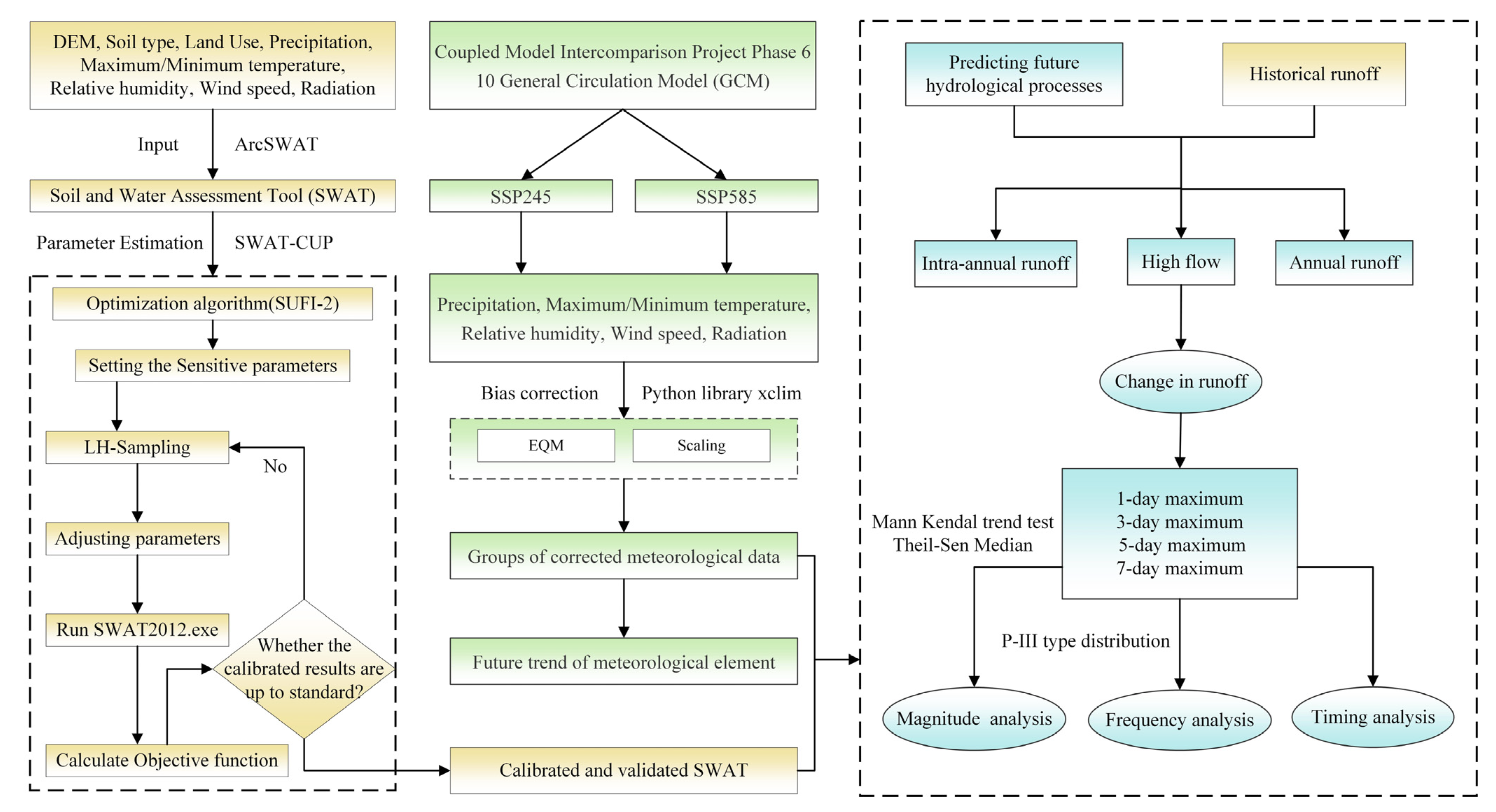
The framework of this study is depicted in Figure 2. The study area is the upper Heihe River basin. The meteorological data based on 10 GCMs from the CMIP6 were used to drive the calibrated SWAT model and project future hydrological processes. In addition to analyzing the changes in future annual and intra-annual runoff, we also extracted the 1-day max, 3-day max, 5-day max, and 7-day max to represent the floods, as used in some previous studies [57,58,59], and then evaluated changes in flood characteristics, i.e., the flood magnitude, frequency, and timing.

3. Results

3.1. SWAT Model Calibration and Validation

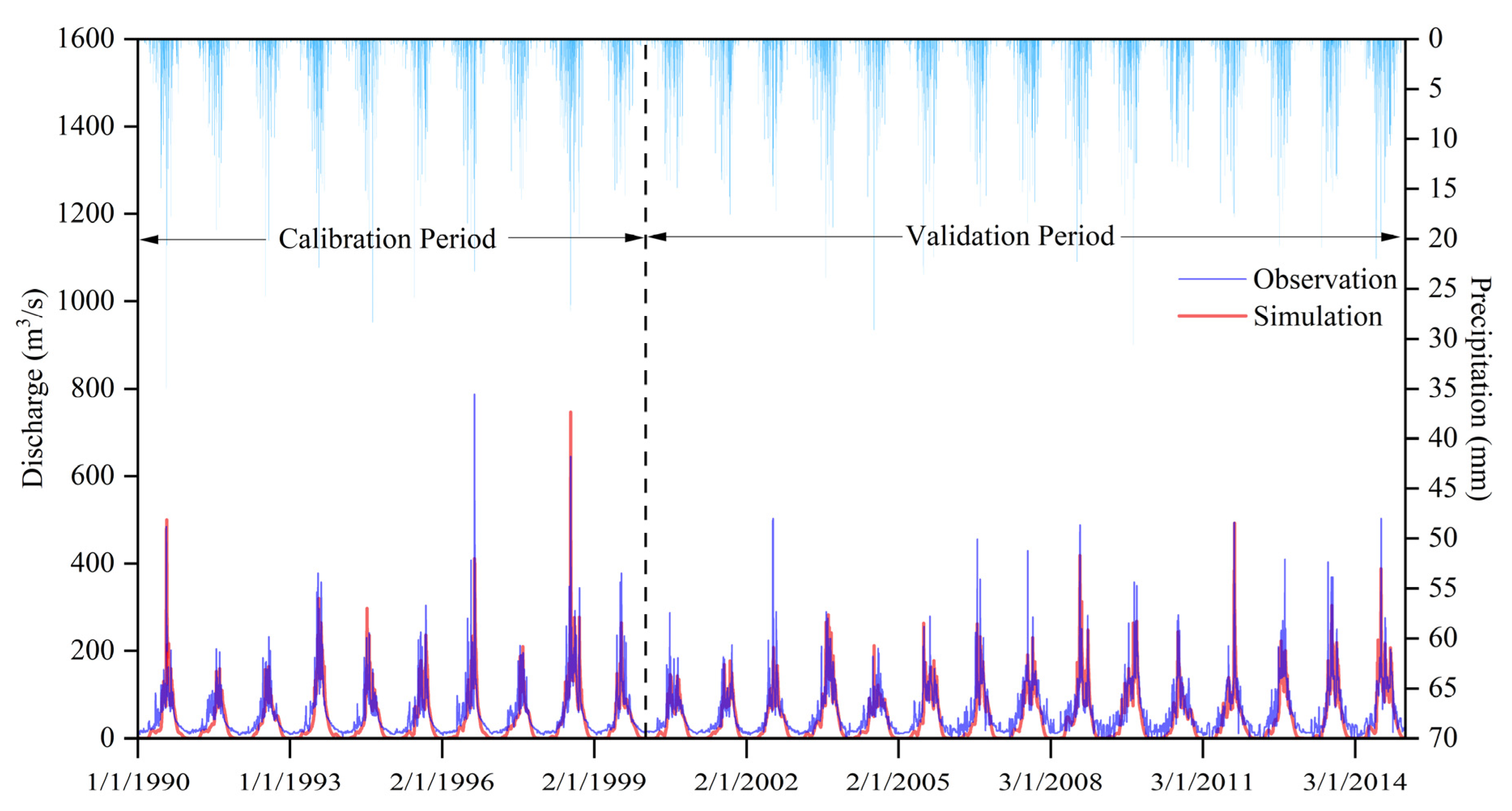
A sensitivity analysis and the study area conditions were used to select the model parameters to be calibrated. The calibration results are listed in Table 4. The time series of the observed and simulated runoff are depicted in Figure 3. The evaluation indicators are listed in Table 5.
Figure 3 shows that the simulated hydrograph derived from the SWAT model is in good agreement with the observed one, and the flow values have a good match. The high flows are simulated with high accuracy, whereas the low flows show slight underestimations.
As shown in Table 5, the R2 is higher than 0.85 for the calibration and validation periods, the NSE is higher than 0.65, the PBIAS is within 30%, and the RSR is less than 0.6. According to the model performance ratings proposed by Moriasi et al. [60], both NSE and RSR achieved a good level. Although PBIAS was slightly higher than the suggested value (within 25% corresponds to a satisfactory level) in the validation period, it was very close to the satisfactory level. These results indicate that the SWAT model performs satisfactorily overall and can be used to project future runoff.
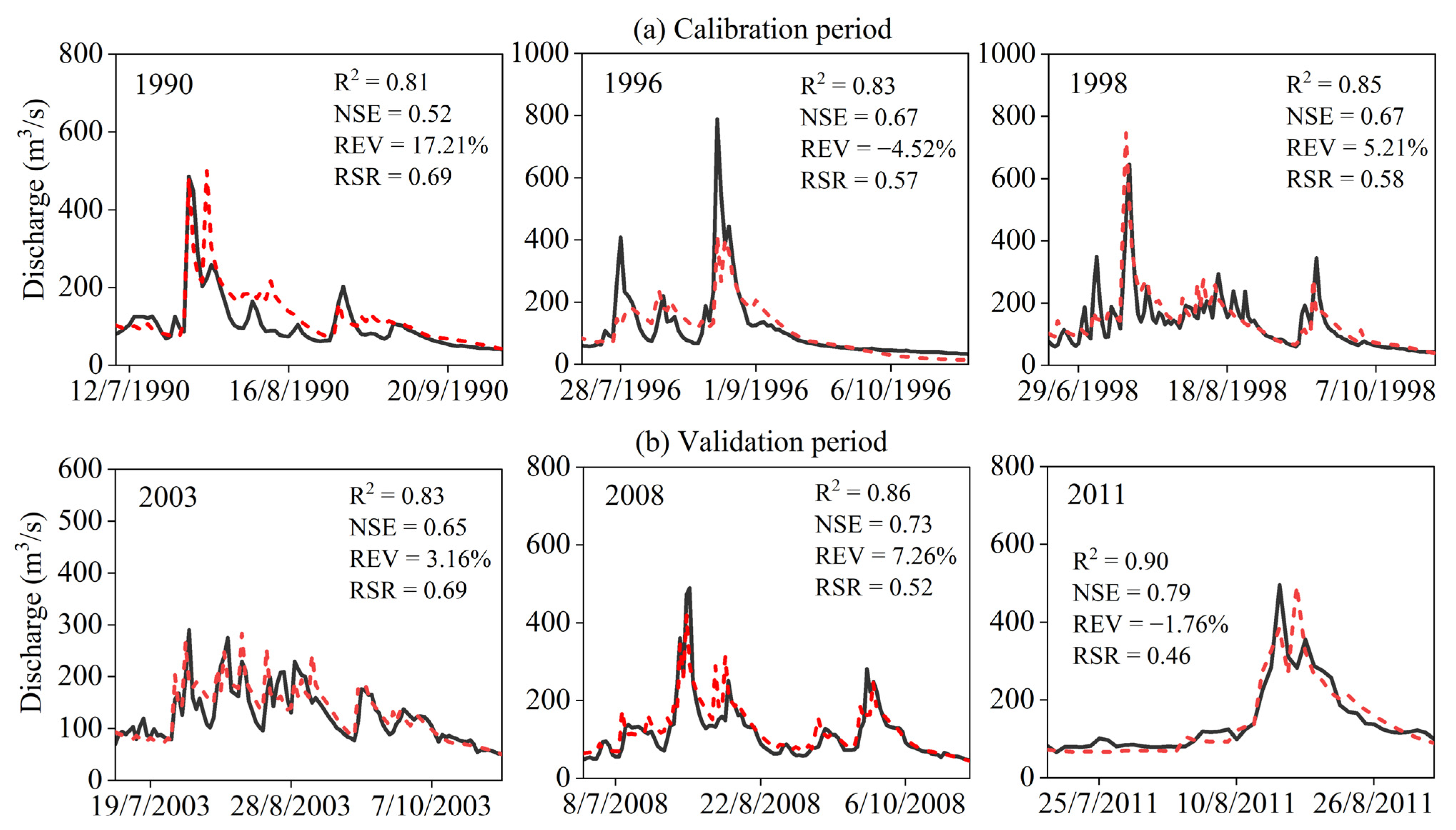
We selected several typical high-flow processes from the calibration and validation periods to investigate the SWAT model’s performance for high-flow simulations, as shown in Figure 4. The results indicate that the model performed well in predicting high flows in 1996 and 1998, with R2 greater than 0.8, NSE greater than 0.65, PBIAS less than 10%, and RSR less than 0.6. The model slightly overestimated the high-flow peak in 1990, resulting in a slightly larger PBIAS and RSR. During the validation period, the SWAT model produced satisfactory results for the high-flow processes in 2003, 2008, and 2011. In general, the simulated flow process closely matched the observed ones, and the trends were relatively consistent, demonstrating that the SWAT model was suitable for projecting future high flows.

3.2. Bias Correction of GCM Outputs

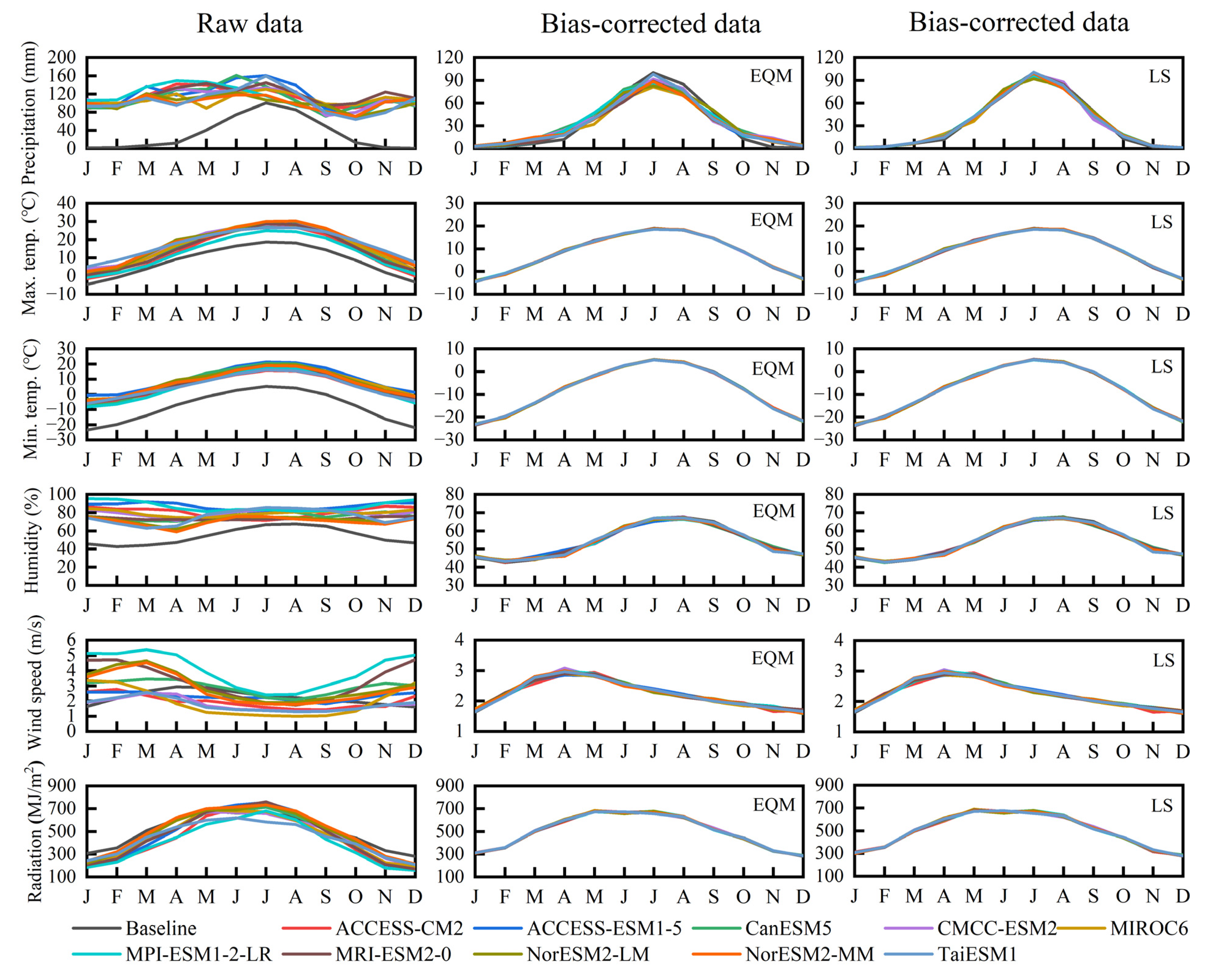
The simulated meteorological data derived from 10 GCMs during 1987–2014 were corrected using the measured data and the EQM and LS methods. Figure 5 shows the original and bias-corrected intra-annual data. All the bias-corrected data showed better agreement with the measured values than the original data. Table 6 shows the results of the mean absolute error (MAE), which is used to represent the difference between the original outputs of the GCMs and those corrected by the two methods. For precipitation, for example, the MAE of the original data ranged from 3.70 to 4.23 mm, and that of the corrected data ranged from 1.59 to 1.70 mm (EQM) and 1.56 to 1.68 mm (LS), respectively. For the maximum temperature, the MAE decreased from 6.42–10.15 °C to 4.09–4.23 °C (EQM) and 4.36 °C to 4.98 °C (LS) after correction. The results demonstrate that LS and EQM are effective for correcting the climate variables of the GCMs, indicating that these correction methods can be used to bias-correct future climate variables.
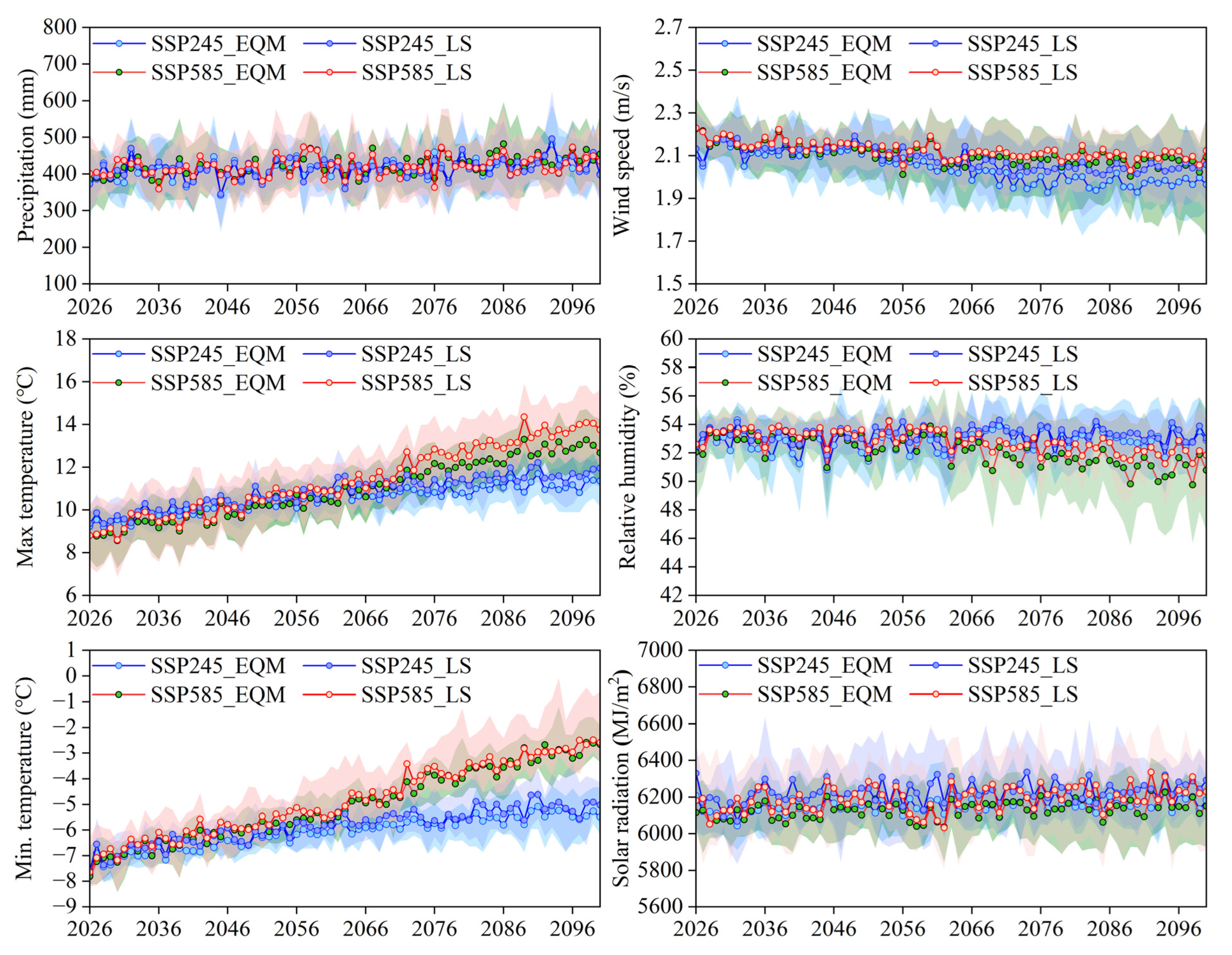
The projections of the six bias-corrected climate variables for 2026 to 2100 are shown in Figure 6. Multi-model ensemble averaging (MMEA) was used to obtain the results, denoted as the solid line with circles. The EQM and LS bias-corrected results show that the future precipitation is projected to increase by 3.8 mm and 3.1 mm per decade under the SSP245 scenario and by 4.0 mm and 3.2 mm, respectively, under the SSP585 scenario. Moreover, this increasing precipitation trend is expected to persist until the end of this century.
The annual maximum temperature is projected to increase by 0.2 °C and 0.3 °C per decade under the SSP245 scenario and by 0.6 °C and 0.7 °C per decade under the SSP585 scenario based on the EQM and LS bias-corrected data, respectively. Similarly, the annual minimum temperature is projected to increase by 0.26 °C and 0.28 °C per decade under the SSP245 scenario and by 0.63 °C and 0. 64 °C per decade under the SSP585 scenario.
The annual mean wind speed is projected to decrease by 0.03 m/s and 0.02 m/s per decade under the SSP245 scenario and by 0.02 m/s and 0.01 m/s per decade under the SSP585 scenario. Similarly, the annual mean relative humidity is expected to decrease under both scenarios. In contrast, solar radiation is projected to increase by 7.0 MJ/m2 and 7.8 MJ/m2 per decade under the SSP245 scenario and by 8.5 MJ/m2 and 12.1 MJ/m2 per decade under the SSP585 scenario.
These results suggest changes in the future climatic variables in the study area. Since large differences will occur in the minimum and maximum temperatures in different periods (Figure 6), the time series from 2026 to 2100 was divided into three parts: the near future from 2026 to 2050 (NF period), the middle future from 2051 to 2075 (MF period), and the far future from 2076 to 2100 (FF period). In the following analysis, we will discuss the hydrological projections in the three periods.
In addition, the results indicate differences in the data corrected by different methods, affecting the projection of hydrological processes in the subsequent modeling. Therefore, using multiple modeling chains to assess potential risks associated with future hydrological processes is essential.

3.3. Runoff Projection

3.3.1. Annual and Intra-Annual Runoff

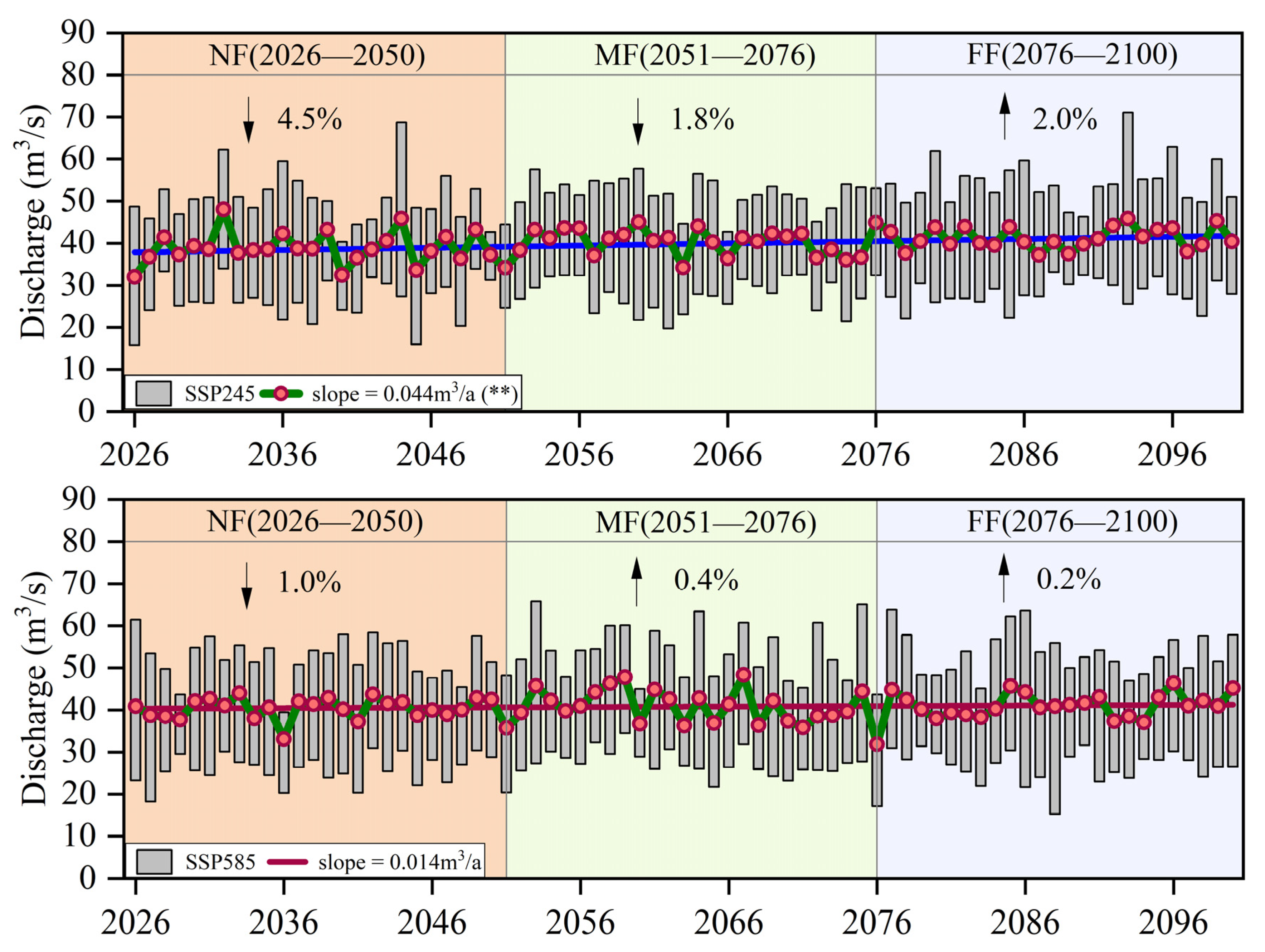
Figure 7 displays the projected annual average runoff in the upper Heihe River basin for the next 75 years. The arrows indicate changes compared to the historical period. The results of the MMEA show that the annual average runoff will be 4.5% and 1.8% lower in the NF and MF periods, respectively, than in the historical period under the SSP245 scenario. In contrast, the runoff will be 2.0% higher in the FF period. In contrast, the runoffs will be 0.4%, 0.2%, and 1.0% lower in the MF, FF, and NF periods, respectively, than in the historical period in the SSP585 scenario. Overall, the long-term runoff in the basin exhibits a declining trend from the historical period to 75 years in the future, with a greater decline under the SSP245 scenario (blue line) and a lesser decline under the SSP585 scenario (red line).
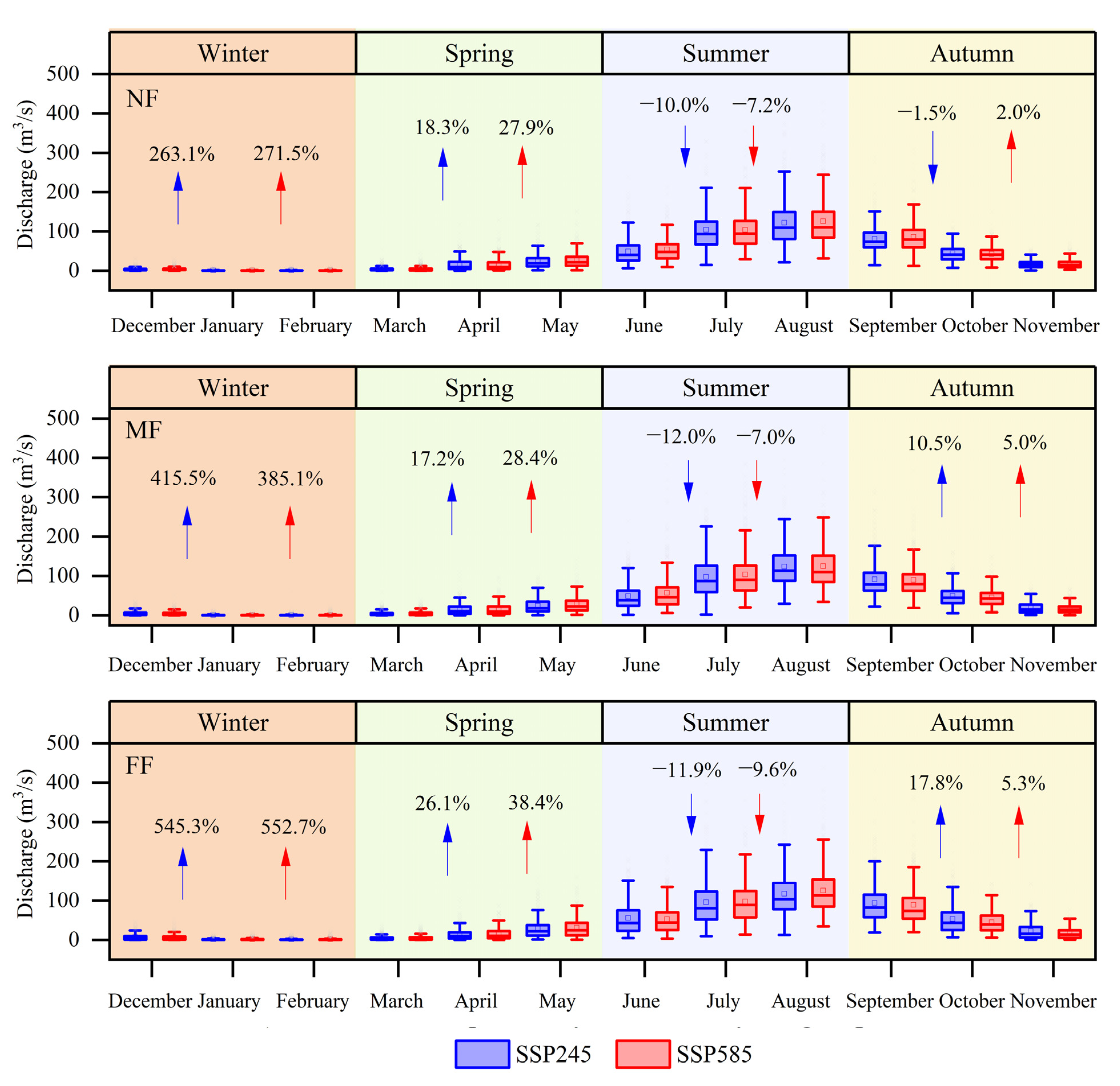
Although the total runoff in the future is projected to either decrease or increase compared to historical periods, there are differences in the changes occurring in different seasons. Figure 8 presents the intra-annual runoff for both scenarios. The results indicate that only the summer runoff is projected to decrease, whereas most of the winter, spring, and autumn runoffs show the opposite trend. In both scenarios, the greatest increase rate in the runoff is observed in winter. This result may be due to the warming temperatures during winter and spring that accelerate the melting of the glacial snowpack. The summer runoff is projected to decrease compared to the historical period. The decrease rates are estimated at 10.0%, 12.0%, and 11.9% in the NF, MF, and FF periods, respectively, in the SSP245 scenario and 7.2% (NF), 7.0% (MF), and 9.6% (FF) in the SSP585 scenario. Autumn exhibits the lowest change rate in the intra-annual runoff.

3.3.2. Magnitude of Floods

Table 7 displays the future discharge and multi-year averages and the results of the Mann–Kendall trend test and Theil–Sen slope estimates. Although the total runoff may decrease or increase in the future for different cases, the flood magnitude is higher in the future. The 1-day max is projected to increase the most under the SSP245 and SSP585 scenarios, with increase rates of 61.9% and 66.4%, respectively. The 3-day max is projected to increase by 34.3% and 38.5%, the 5-day max is projected to increase by 22.6% and 26.2%, and the 7-day max is projected to increase the least, by 18.7% and 22.5% under the two scenarios, respectively.
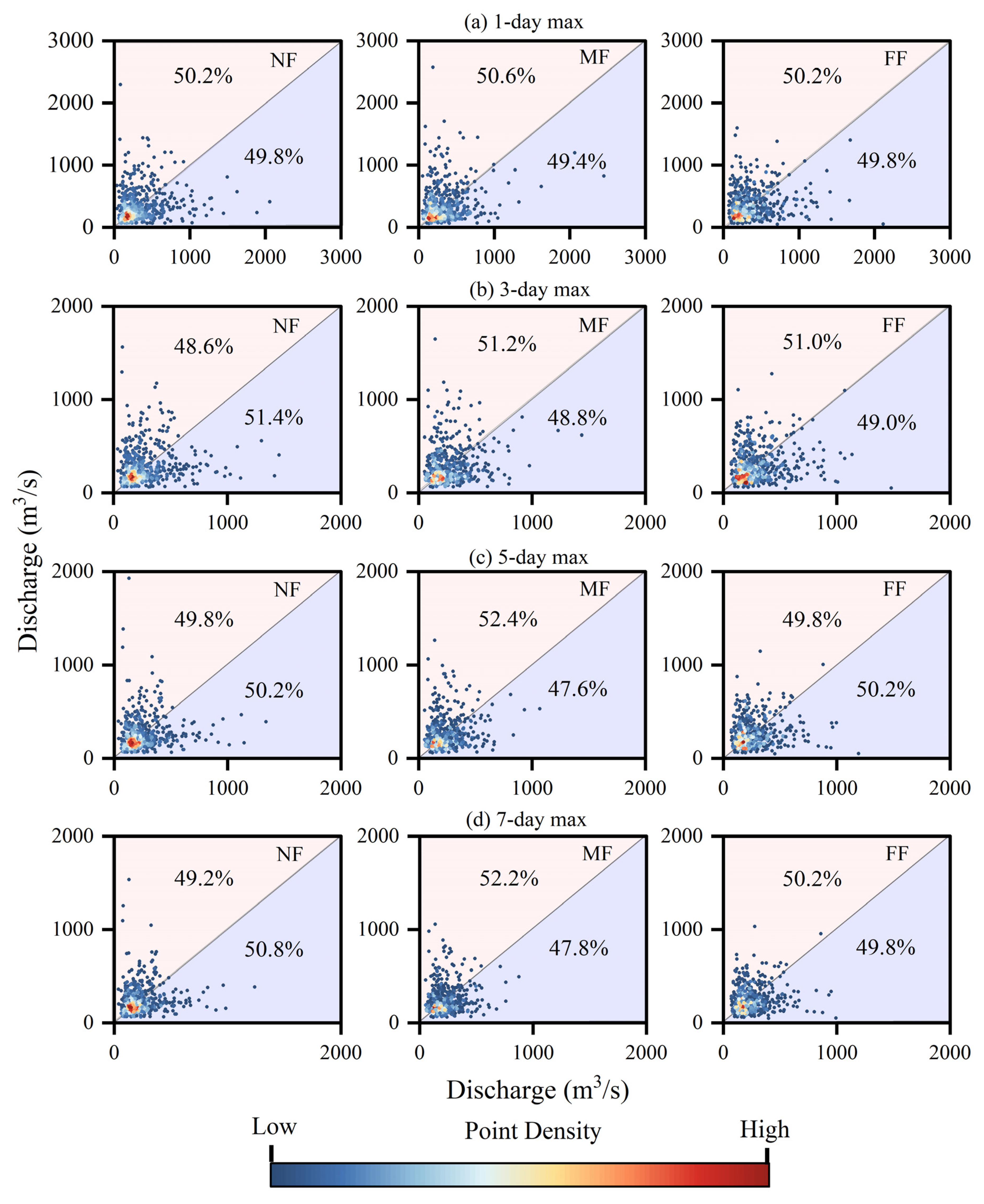
We created scatter plots between the flood magnitudes for the two scenarios (Figure 9). When the points are located below the forty-five-degree line, the SSP585 scenario has higher flows than the SSP245 scenario and vice versa.
Slightly more points are located in the pink area than in the blue area for the 1-day max, indicating a slightly higher probability of floods occurring under the SSP245 scenario. For the 3-day, 5-day, and 7-day max, slightly higher likelihoods of floods occur under the SSP585 scenario during the NF period, and higher likelihoods occur under the SSP245 scenario during the MF period. Most of the points are clustered in the flow range of 100–500 m3/s, indicating that this flood magnitude will occur more frequently in the future.

3.3.3. Frequency of Floods

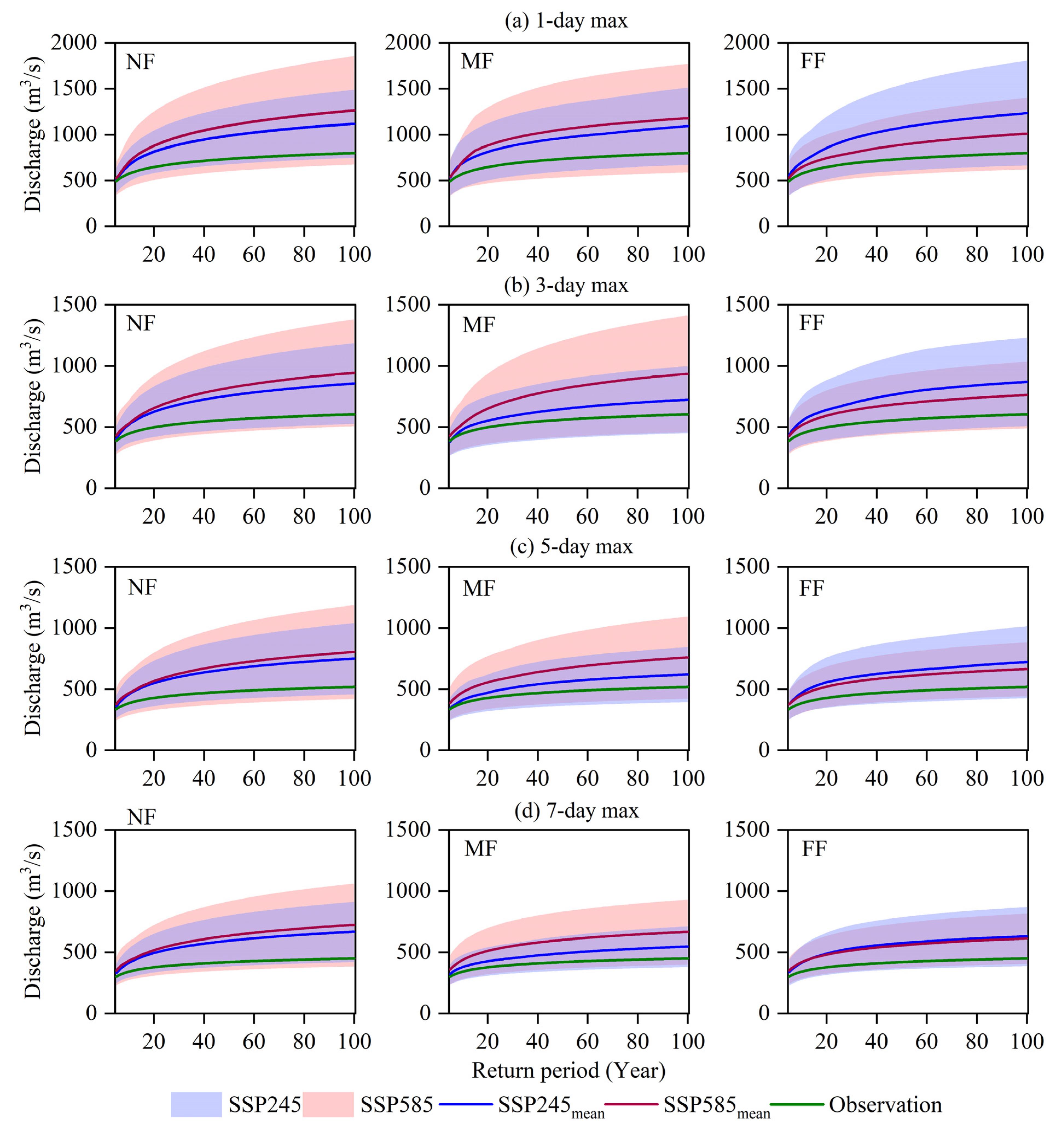
We calculated the flood frequency under different return periods (5 years to 100 years) using the Pearson type III theoretical distribution to assess the impact of climate change on flood frequency (Figure 10). The shaded part represents the 10th to 90th percentile ranges of the projections, and the solid line represents the magnitude of MMEA. The results show that the flood frequency will be significantly higher in the future than in the historical period for different return periods. Therefore, an early warning system should be implemented.
Table 8 lists the flood magnitudes in the historical period and the future. The 1-day max for the 30-, 50-, 80-, and 100-year return periods are expected to increase by an average of 26.3%, 30.72%, 34.9%, and 36.1% under the SSP245 scenario and by 35.0%, 40.7%, 46.2%, and 47.6%, respectively, under the SSP585 scenario. The 3-day max for the four return periods is expected to increase by 23.6%, 27.6%, 31.0%, and 32.5% under the SSP245 scenario and by 30.8%, 35.5%, 39.4%, and 41.1%, respectively, under the SSP585 scenario. As the return period increases, the rate of increase in the flood magnitude increases. The SSP585 scenario always exhibits a higher rate of increase in the NF and MF periods, indicating a higher flood risk.
Higher-magnitude floods will occur in the NF period than in the MF and FF periods. For example, the 1-day max for the 100-year return period will increase by 44.7% in the NF period under the SSP245 scenario. In the same scenario, the FF period will experience the second-largest increase (39.2%), followed by the MF period (24.3%).
Figure 10 also shows that the flood projection intervals for the two scenarios are similar for shorter return periods, indicating that the flood projections with shorter return periods are less sensitive to both scenarios, whereas with the return period increasing, the sensitivity is also shown to increase. The larger the flood projection intervals, the greater the uncertainties.

3.3.4. Timing of Floods

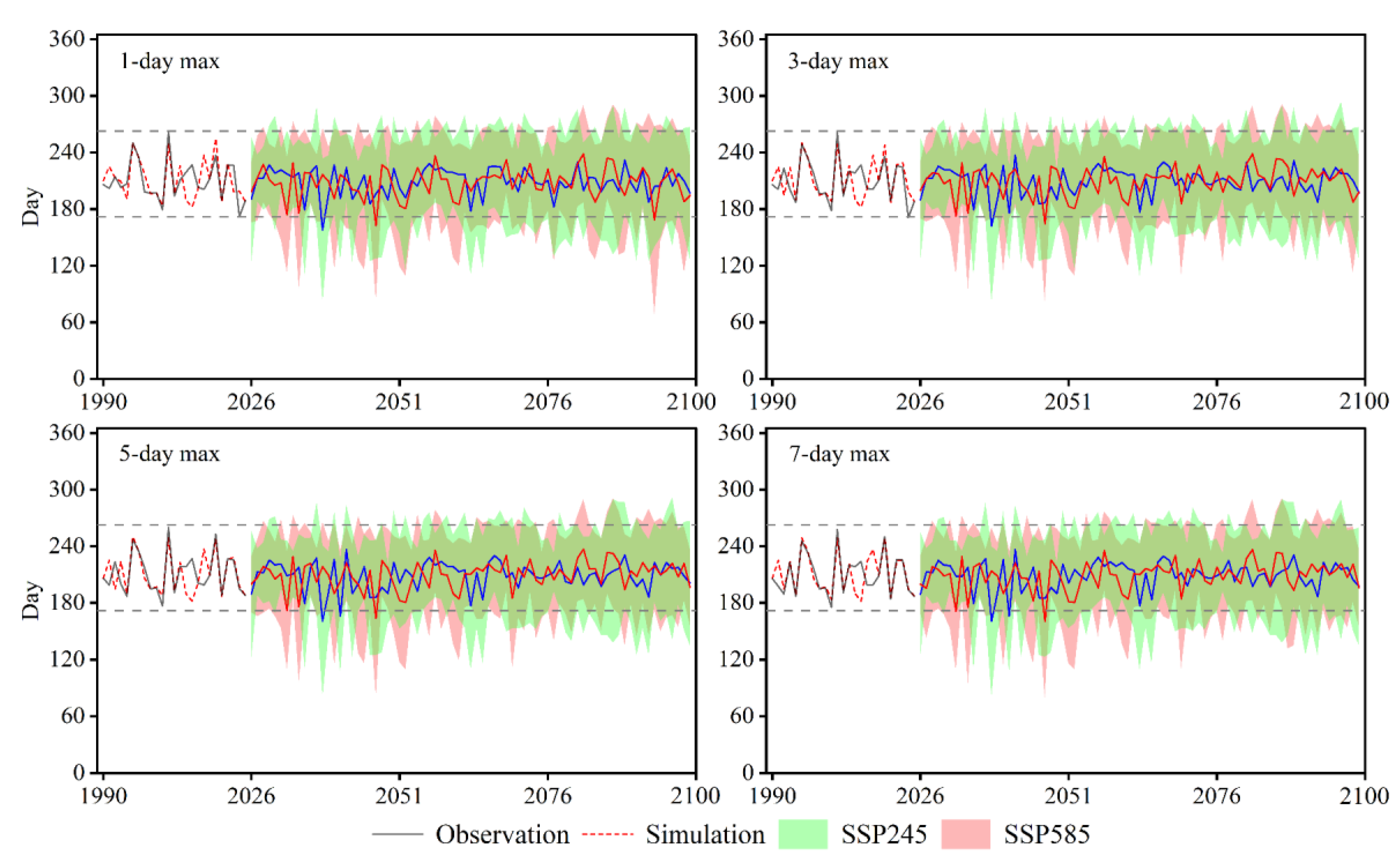
We analyzed and compared the maximum flow occurrences over one, three, five, and seven days in the future and historical periods, as shown in Figure 11. The shaded part represents the flood occurrence time derived from all GCMs, and the solid line represents the average occurrence time obtained from the MMEA. Most of the floods occurred in June, July, August, and early September (171–260 days). The future floods are projected to occur sooner or later than the historical floods.
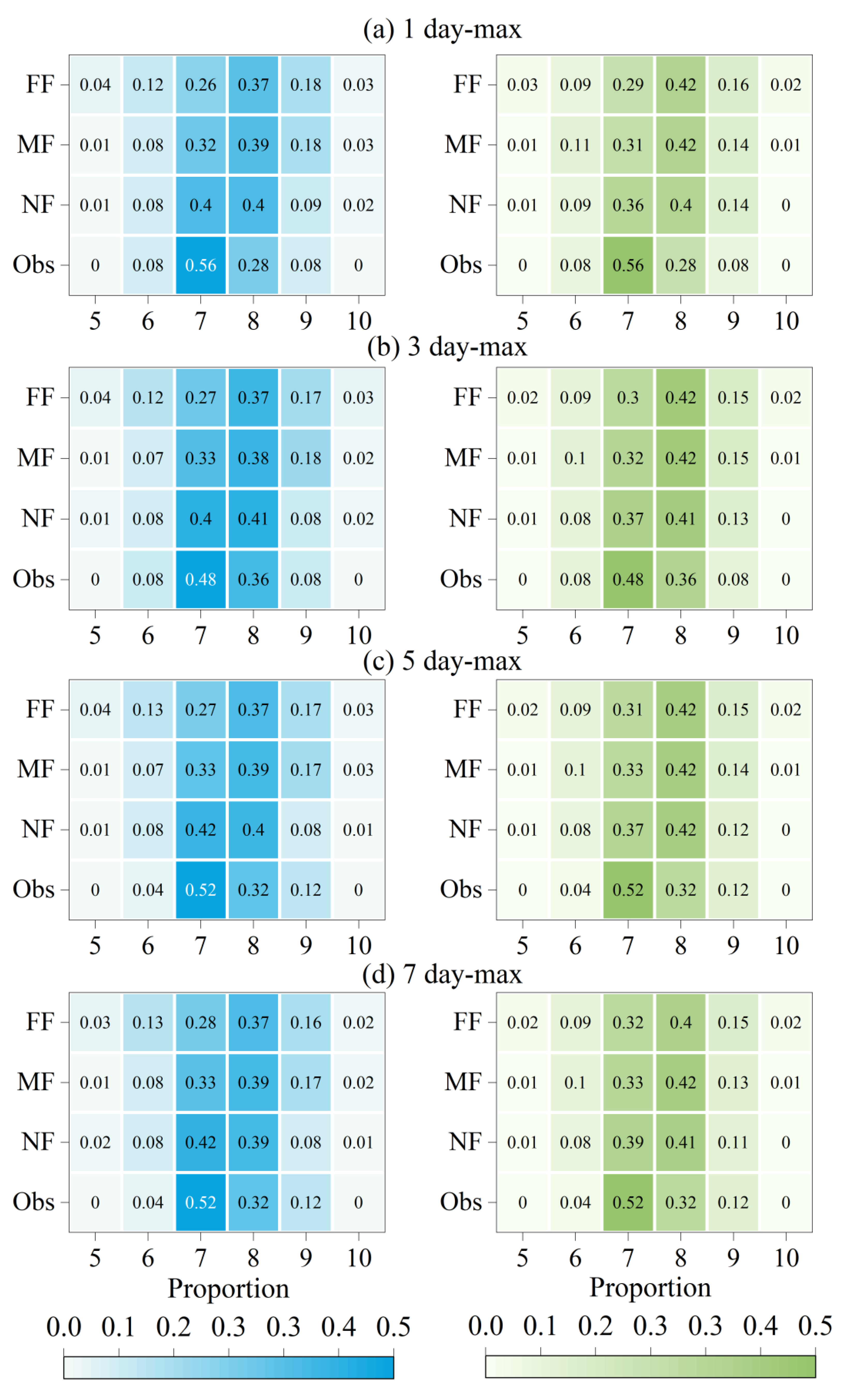
We generated 40 time series of future runoff events using the 2 future scenarios, 10 GCMs, and 2 bias-correction methods. We extracted the flood timing and classified the results into six groups based on the month of flood occurrence. Figure 12 shows the flood probability in different months. Most floods occurred between July and September in the historical period, with the highest probability in July. The probabilities were 56%, 48%, 52%, and 52% in July and 28%, 36%, 32%, and 32% in August for the 1-day max, 3-day max, 5-day max, and 7-day max, respectively.
The flood probabilities were different in the future period. The probabilities were lower in July and higher in August. The future flood probabilities in July were 32.7% (1-day max), 33.3% (3-day max), 34.0% (5-day max), and 34.3% (7-day max) in the SSP245 scenario and 32.0% (1-day max), 33.0% (3-day max), 33.7% (5-day max), and 34.7% (7-day max) in the SSP585 scenario. The flood probabilities in August were 38.7% (1-day max), 38.7% (3-day max), 38.7% (5-day max), and 38.3% (7-day max) in the SSP245 scenario and 41.3% (1-day max), 41.7% (3-day max), 42.0% (5-day max), and 41.0% (7-day max) in the SSP585 scenario. Overall, the flood probability in August is expected to increase from 32% in the past to 40% in the future; thus, most floods will occur in August. Furthermore, the flood probability in August is higher for the SSP585 scenario than for the SSP245 scenario.
The flood probabilities are also projected to increase in May, June, September, and October, especially during the MF and FF periods. Specifically, the flood probabilities in September are expected to increase from 8% to 14–18% for the 1-day max and 3-day max and from 12% to 13–17% for the 5-day max and 7-day max. Floods did not occur in May historically but may occur in this month in the future, although the probability is projected to be relatively low.
Overall, the flood occurrence time will have a larger range in the future, with the highest probability in August, lagging one month behind that of the historical period.

4. Discussion

4.1. Impacts of Climate Change on Annual and Intra-Annual Runoff

The results of this study suggest that the upper Heihe River basin may experience warmer and wetter conditions in the future. This finding aligns with previous studies. For instance, Wu et al. [61] and Li et al. [35] found that this basin will likely experience higher temperatures and precipitation in the future. In addition, recent studies have revealed that glaciers in the Qilian Mountains region in the upper Heihe River have been retreating due to increasing temperatures over the past few decades [19,61,62,63]. As a result, more runoff from glacial meltwater has occurred in the upper Heihe River basin, a process that is expected to intensify with continued warming in the future [19,64].
In our study, the multi-year average runoff in the future was projected to decrease in some cases (the NF and MF periods under the SSP245 scenario and the FF period under the SSP585 scenario) and increase in other cases, which is not consistent with the results obtained from previous studies, which observed an increase in total runoff [36,37]. The reasons may include the use of different GCMs, hydrological models, and study periods. The results of several GCMs in our study showed increasing trends in the future runoff compared to the historical period (Figure 7 and Figure 8). We chose MMEA to estimate the changes in runoff. This approach has been widely used by many researchers to analyze the impact of climate change on watershed hydrological processes [20,64,65].
The results of the MMEA indicate that the multi-year average annual evapotranspiration rate is much higher than the precipitation rate during the NF and MF periods under the SSP245 scenario and the NF period under the SSP585 scenario, indicating a decrease in runoff in these periods. However, the precipitation rate was slightly higher than the evapotranspiration rate during the FF period under the SSP245 scenario, which may lead to the runoff increasing.
The intra-annual runoff results indicate that the winter and spring runoffs are projected to increase, whereas the summer runoff is projected to decrease, which agrees with the results of Li et al. [37]. The increases in the winter and spring runoffs may be attributed to the increased seasonal precipitation and temperature (Section 4.2), producing more rainfall and snowmelt runoff.
The summer runoff (June, July, and August) is expected to decrease. The precipitation, evapotranspiration, and snowmelt data in the historical and future periods are shown in Figure 13. The decrease in runoff in June under the SSP245 scenario may attributed to the reduction in precipitation and snowmelt, the decrease in July may due to a decrease in precipitation, and the decrease in August may related to an increase in evapotranspiration. In contrast, the decrease in runoff in June under the SSP585 scenario may attributed to higher evapotranspiration and less snowmelt, whereas the decreases in July and August may attributed to higher evapotranspiration.

4.2. Impact of Climate Change on Floods

Precipitation and temperature affect intra-annual runoff and flood occurrence. Previous studies have suggested that changes in precipitation and evapotranspiration can impact the flood magnitude. Increased precipitation can potentially cause greater flooding, and decreased precipitation and increased evapotranspiration may lead to less flooding [11,14]. The upper Heihe River basin is located in the Qilian Mountains, which have high elevations. Thus, it is speculated that summer floods in the basin may caused by precipitation and glacier/snow melting, and spring floods may primarily caused by glacier/snow melting due to rising temperatures. The primary contributing factors to increased flood magnitudes in the future are speculated to be the increased precipitation and accelerated snow melting caused by climate change.
Similar to the historical period, most floods (over 75%) in the future are expected to occur during summer. However, the reduction in precipitation and the increase in evapotranspiration in July are projected to result in a substantial reduction in the flood magnitude in July, and the proportion of floods in August is expected to increase in the future. This study also reveals that the flood is projected to occur during spring in the future, which is unprecedented in the historical period. The likely reason is that snow melting is projected to occur earlier due to rising temperatures. Stewart et al. demonstrated that a temperature rise of 1 to 3 °C during spring caused the onset of snowmelt runoff to advance by 1 to 4 weeks [66,67]. Thus, the rising temperatures in the future would lead to earlier snowmelt runoff and more snow melting in the basin. Therefore, it is necessary to remain vigilant of major flooding in the future that could be caused by warmer spring temperatures and higher rainfall.

5. Conclusions

The study used 10 GCMs under two scenarios in the CMIP6 and two downscaling methods to generate future climatic data for the upper Heihe River basin. The SWAT model was used to project future hydrological processes and potential floods in the basin. The main findings of the study are as follows:
(1)
Climate change will affect the annual and intra-annual runoff in the basin. The change in the annual average runoff will be −4.5% (NF), −1.8% (MF), and +2.0% (FF) under the SSP245 scenario and −1.0% (NF), +0.4% (MF), and +0.2% (FF) under the SSP585 scenario. Winter and spring runoff is projected to increase due to more precipitation and snowmelt, whereas summer runoff is projected to decrease due to less rainfall and snowmelt and more evapotranspiration.
(2)
The MMEA’s projections show that the basin will experience higher flood magnitudes in the future. The 1-day maximum flow is expected to increase the most under the SSP245 and SSP585 scenarios (61.9% and 66.4%, respectively) compared to the historical period. The 3-day, 5-day, and 7-day maximum flow rates are also projected to increase under both scenarios, with increases ranging from 18.7% to 38.5%.
(3)
The flood frequency is projected to increase in the future, particularly in the NF period. The 1-day maximum flow is expected to increase by 44.72% and 63.72% under the SSP245 and SSP585 scenarios, respectively.
(4)
The flood timing is also expected to change, with the highest probability occurring from July to August. Additionally, there will be more flood events occurring in other months in the future.
There are also some limitations to this study; for example, current studies pointed out that the response of runoff to climate change may be different between models calibrated using observed data and those calibrated through the output of GCMs [28,68]. In this study, only the observed meteorological data were used to calibrate the model, which may introduce a certain degree of bias, especially in projecting extreme hydrological events. In addition, future runoff predictions are often subject to large uncertainties due to choices made during the modeling process, e.g., GCMs, emission scenarios, hydrological models, different sources of data, etc. [23,24,25,26,27,69,70]. Research has indicated that the selection of scenarios can significantly affect watersheds with snowmelt [27], and the uncertainty associated with GCMs plays a crucial role in predicting high and average flows [69,70]. The coupling between climate change projection and hydrological models is also one source of such uncertainties [28]. Thus, more diverse scenarios, GCMs, and modeling options to conduct a more comprehensive analysis of hydrological processes are required in future studies.

Author Contributions

Conceptualization, Z.L. (Zhanling Li) and Y.Y.; methodology, Y.Y.; software, Y.Y.; validation, Z.L. (Zhanling Li) and Y.Y.; formal analysis, Z.L. (Zhanling Li) and Y.Y.; investigation, Z.L. (Zhanling Li), Y.Y. and X.L.; resources, Z.L. (Zhanling Li); data curation, Y.Y. and X.L.; writing—original draft preparation, Y.Y.; writing—review and editing, Z.L. (Zhanling Li) and Z.L. (Zhanjie Li); visualization, Y.Y.; supervision, Z.L. (Zhanling Li) and Z.L. (Zhanjie Li); project administration, Z.L. (Zhanling Li); funding acquisition, Z.L. (Zhanling Li). All authors have read and agreed to the published version of the manuscript.

Funding

This study was supported by the Belt and Road Special Foundation of the State Key Laboratory of Hydrology-Water Resources and Hydraulic Engineering (2021nkms03).

Institutional Review Board Statement

Not applicable.

Informed Consent Statement

Not applicable.

Data Availability Statement

The GCM datasets used in this study can be downloaded from the Earth System Grid Federation (ESGF) website (https://esgf-node.llnl.gov/projects/cmip6/) (accessed on 22 March 2023). The runoff datasets in the study area are unavailable due to privacy.

Conflicts of Interest

The authors declare no conflict of interest.

References

  1. Kundzewicz, Z.W.; Kanae, S.; Seneviratne, S.I.; Handmer, J.; Nicholls, N.; Peduzzi, P.; Mechler, R.; Bouwer, L.M.; Arnell, N.; Mach, K.; et al. Flood Risk and Climate Change: Global and Regional. Hydrol. Sci. J. 2014, 59, 1–28. [Google Scholar] [CrossRef] [Green Version]
  2. Barredo, J.I. Natural Hazards and Earth System Sciences Normalised Flood Losses in Europe: 1970–2006. Hazards Earth Syst. Sci. 2009, 9, 97–104. [Google Scholar] [CrossRef]
  3. Berghuijs, W.R.; Woods, R.A.; Hutton, C.J.; Sivapalan, M. Dominant Flood Generating Mechanisms across the United States. Geophys. Res. Lett. 2016, 43, 4382–4390. [Google Scholar] [CrossRef] [Green Version]
  4. Mitigation of Climate Change Climate Change 2022 Working Group III Contribution to the Sixth Assessment Report of the Intergovernmental Panel on Climate Change; Cambridge University Press: Cambridge, UK, 2022; ISBN 9789291691609.
  5. Gudmundsson, L.; Bremnes, J.B.; Haugen, J.E.; Engen-Skaugen, T. Technical Note: Downscaling RCM Precipitation to the Station Scale Using Statistical Transformations – A Comparison of Methods. Hydrol. Earth Syst. Sci. 2012, 16, 3383–3390. [Google Scholar] [CrossRef] [Green Version]
  6. Pokhrel, Y.; Felfelani, F.; Satoh, Y.; Boulange, J.; Burek, P.; Gädeke, A.; Gerten, D.; Gosling, S.N.; Grillakis, M.; Gudmundsson, L.; et al. Global Terrestrial Water Storage and Drought Severity under Climate Change. Nat. Clim. Chang. 2021, 11, 226–233. [Google Scholar] [CrossRef]
  7. Yang, P.; Zhang, S.; Xia, J.; Zhan, C.; Cai, W.; Wang, W.; Luo, X.; Chen, N.; Li, J. Analysis of Drought and Flood Alternation and Its Driving Factors in the Yangtze River Basin under Climate Change. Atmos. Res. 2022, 270, 105536. [Google Scholar] [CrossRef]
  8. Wang, X.; Chen, R.; Li, K.; Yang, Y.; Liu, J.; Liu, Z.; Han, C. Trends and Variability in Flood Magnitude: A Case Study of the Floods in the Qilian Mountains, Northwest China. Atmosphere 2023, 14, 557. [Google Scholar] [CrossRef]
  9. Ekolu, J.; Dieppois, B.; Sidibe, M.; Eden, J.M.; Tramblay, Y.; Villarini, G.; Peña-Angulo, D.; Mahé, G.; Paturel, J.E.; Onyutha, C.; et al. Long-Term Variability in Hydrological Droughts and Floods in Sub-Saharan Africa: New Perspectives from a 65-Year Daily Streamflow Dataset. J. Hydrol. 2022, 613, 128359. [Google Scholar] [CrossRef]
  10. Peng, Y.; Wang, Z.; Cui, Y.; Su, Y.; Tang, Y.; Luo, S.; Liu, L.; Zhou, Y.; Dong, J.; Wang, W.; et al. Prediction of Drought/Flood Intensities Based on a 500-Year Time Series in Three Different Climate Provinces of China. Reg. Environ. Chang. 2022, 22, 80. [Google Scholar] [CrossRef]
  11. Tabari, H.; Abghari, H.; Hosseinzadeh Talaee, P. Temporal Trends and Spatial Characteristics of Drought and Rainfall in Arid and Semiarid Regions of Iran. Hydrol. Process. 2012, 26, 3351–3361. [Google Scholar] [CrossRef]
  12. Konisky, D.M.; Hughes, L.; Kaylor, C.H. Extreme Weather Events and Climate Change Concern. Clim. Chang. 2016, 134, 533–547. [Google Scholar] [CrossRef]
  13. Guo, H.; Bao, A.; Liu, T.; Jiapaer, G.; Ndayisaba, F.; Jiang, L.; Kurban, A.; De Maeyer, P. Spatial and Temporal Characteristics of Droughts in Central Asia during 1966–2015. Sci. Total Environ. 2018, 624, 1523–1538. [Google Scholar] [CrossRef]
  14. Zhao, Y.; Weng, Z.; Chen, H.; Yang, J. Analysis of the Evolution of Drought, Flood, and Drought-Flood Abrupt Alternation Events under Climate Change Using the Daily SWAP Index. Water 2020, 12, 1969. [Google Scholar] [CrossRef]
  15. Zhang, J.; Zhao, P.; Zhang, Y.; Cheng, L.; Song, J.; Fu, G.; Wang, Y.; Liu, Q.; Lyu, S.; Qi, S.; et al. Long-Term Baseflow Responses to Projected Climate Change in the Weihe River Basin, Loess Plateau, China. Remote Sens. 2022, 14, 5097. [Google Scholar] [CrossRef]
  16. Kundzewicz, Z.W.; Schellnhuber, H.-J. Floods in the IPCC TAR Perspective. Nat. Hazards 2004, 31, 111–128. [Google Scholar] [CrossRef]
  17. Wang, H.; Jiang, P.; Zhang, R.; Zhao, J.; Si, W.; Fang, Y.; Zhang, N. The Changing Precipitation Storm Properties under Future Climate Change. Hydrol. Res. 2023, 54, 580–590. [Google Scholar] [CrossRef]
  18. Eingrüber, N.; Korres, W. Climate Change Simulation and Trend Analysis of Extreme Precipitation and Floods in the Mesoscale Rur Catchment in Western Germany until 2099 Using Statistical Downscaling Model (SDSM) and the Soil & Water Assessment Tool (SWAT Model). Sci. Total Environ. 2022, 838, 155775. [Google Scholar] [CrossRef]
  19. Wang, X.; Chen, R.; Li, H.; Li, K.; Liu, J.; Liu, G. Detection and Attribution of Trends in Flood Frequency under Climate Change in the Qilian Mountains, Northwest China. J. Hydrol. Reg. Stud. 2022, 42, 101153. [Google Scholar] [CrossRef]
  20. Yang, S.; Yang, D.; Zhao, B.; Ma, T.; Lu, W.; Santisirisomboon, J. Future Changes in High and Low Flows under the Impacts of Climate and Land Use Changes in the Jiulong River Basin of Southeast China. Atmosphere 2022, 13, 150. [Google Scholar] [CrossRef]
  21. Xiang, Y.; Wang, Y.; Chen, Y.; Zhang, Q. Impact of Climate Change on the Hydrological Regime of the Yarkant River Basin, China: An Assessment Using Three SSP Scenarios of CMIP6 GCMs. Remote Sens. 2022, 14, 115. [Google Scholar] [CrossRef]
  22. Iqbal, M.S.; Dahri, Z.H.; Querner, E.P.; Khan, A.; Hofstra, N. Impact of Climate Change on Flood Frequency and Intensity in the Kabul River Basin. Geosciences 2018, 8, 114. [Google Scholar] [CrossRef] [Green Version]
  23. Bosshard, T.; Carambia, M.; Goergen, K.; Kotlarski, S.; Krahe, P.; Zappa, M.; Schär, C. Quantifying Uncertainty Sources in an Ensemble of Hydrological Climate-Impact Projections. Water Resour. Res. 2013, 49, 1523–1536. [Google Scholar] [CrossRef] [Green Version]
  24. Chen, J.; Brissette, F.P.; Poulin, A.; Leconte, R. Overall Uncertainty Study of the Hydrological Impacts of Climate Change for a Canadian Watershed. Water Resour. Res. 2011, 47, W12509. [Google Scholar] [CrossRef]
  25. Wilby, R.L.; Harris, I. A Framework for Assessing Uncertainties in Climate Change Impacts: Low-Flow Scenarios for the River Thames, UK. Water Resour. Res. 2006, 42, W02419. [Google Scholar] [CrossRef]
  26. Addor, N.; Rössler, O.; Köplin, N.; Huss, M.; Weingartner, R.; Seibert, J. Robust Changes and Sources of Uncertainty in the Projected Hydrological Regimes of Swiss Catchments. Water Resour. Res. 2014, 50, 7541–7562. [Google Scholar] [CrossRef] [Green Version]
  27. Chegwidden, O.S.; Nijssen, B.; Rupp, D.E.; Arnold, J.R.; Clark, M.P.; Hamman, J.J.; Kao, S.C.; Mao, Y.; Mizukami, N.; Mote, P.W.; et al. How Do Modeling Decisions Affect the Spread Among Hydrologic Climate Change Projections? Exploring a Large Ensemble of Simulations Across a Diversity of Hydroclimates. Earths Future 2019, 7, 623–637. [Google Scholar] [CrossRef] [Green Version]
  28. Majone, B.; Avesani, D.; Zulian, P.; Fiori, A.; Bellin, A. Analysis of High Streamflow Extremes in Climate Change Studies: How Do We Calibrate Hydrological Models? Hydrol. Earth Syst. Sci. 2022, 26, 3863–3883. [Google Scholar] [CrossRef]
  29. Beckers, J.; Smerdon, B.; Wilson, M. FORREX. Review of Hydrologic Models for Forest Management and Climate Change Applications in British Columbia and Alberta. Forrex Ser. 2009, 25, 29–38. [Google Scholar]
  30. Nikam, B.R.; Garg, V.; Jeyaprakash, K.; Gupta, P.K.; Srivastav, S.K.; Thakur, P.K.; Aggarwal, S.P. Analyzing Future Water Availability and Hydrological Extremes in the Krishna Basin under Changing Climatic Conditions. Arab. J. Geosci. 2018, 11, 581. [Google Scholar] [CrossRef]
  31. Jackson, B.; Mcintyre, N.; Pechlivanidis, I.G.; Jackson, B.M.; Mcintyre, N.R.; Wheater, H.S. Catchment Scale Hydrological Modelling: A Review of Model Types, Calibration Approaches and Uncertainty Analysis Methods in the Context of Recent Developments in Technology and Applications. Artic. Glob. NEST Int. J. 2011, 13, 193–214. [Google Scholar] [CrossRef]
  32. The CMIP6 Landscape. Nat. Clim. Chang. 2019, 9, 727. [CrossRef] [Green Version]
  33. Pascoe, C.; Lawrence, B.N.; Guilyardi, E.; Juckes, M.; Taylor, K.E. Documenting Numerical Experiments in Support of the Coupled Model Intercomparison Project Phase 6 (CMIP6). Geosci. Model Dev. 2020, 13, 2149–2167. [Google Scholar] [CrossRef]
  34. Eyring, V.; Bony, S.; Meehl, G.A.; Senior, C.A.; Stevens, B.; Stouffer, R.J.; Taylor, K.E. Overview of the Coupled Model Intercomparison Project Phase 6 (CMIP6) Experimental Design and Organization. Geosci. Model Dev. 2016, 9, 1937–1958. [Google Scholar] [CrossRef] [Green Version]
  35. Li, Z.; Li, Q.; Wang, J.; Feng, Y.; Shao, Q. Impacts of Projected Climate Change on Runoff in Upper Reach of Heihe River Basin Using Climate Elasticity Method and GCMs. Sci. Total Environ. 2020, 716, 137072. [Google Scholar] [CrossRef]
  36. Zhang, A.; Liu, W.; Yin, Z.; Fu, G.; Zheng, C. How Will Climate Change Affect the Water Availability in the Heihe River Basin, Northwest China? J. Hydrometeorol. 2016, 17, 1517–1542. [Google Scholar] [CrossRef]
  37. Li, Z.; Li, W.; Li, Z.; Lv, X. Responses of Runoff and Its Extremes to Climate Change in the Upper Catchment of the Heihe River Basin, China. Atmosphere 2023, 14, 539. [Google Scholar] [CrossRef]
  38. Jiménez-Navarro, I.C.; Jimeno-Sáez, P.; López-Ballesteros, A.; Pérez-Sánchez, J.; Senent-Aparicio, J. Impact of Climate Change on the Hydrology of the Forested Watershed That Drains to Lake Erken in Sweden: An Analysis Using Swat+ and Cmip6 Scenarios. Forests 2021, 12, 1803. [Google Scholar] [CrossRef]
  39. Liang, Y.; Liu, L.; Xu, Z. An Integrated Modelling Approach Inmountainous Watershed of Heihe River Basin, Northwest China. Nat. Resour. 2014, 5, 90–98. [Google Scholar] [CrossRef]
  40. Song, X.; Liu, Y.; Zhong, F.; Deng, X.; Qi, Y.; Zhang, J.; Zhang, R.; Zhang, Y. Payment Criteria and Mode for Watershed Ecosystem Services: A Case Study of the Heihe River Basin, Northwest China. Sustainability 2020, 12, 6177. [Google Scholar] [CrossRef]
  41. Zhang, A.; Zheng, C.; Wang, S.; Yao, Y. Analysis of Streamflow Variations in the Heihe River Basin, Northwest China: Trends, Abrupt Changes, Driving Factors and Ecological Influences. J. Hydrol. Reg. Stud. 2015, 3, 106–124. [Google Scholar] [CrossRef] [Green Version]
  42. Luo, K.; Tao, F.; Deng, X.; Moiwo, J.P. Changes in Potential Evapotranspiration and Surface Runoff in 1981–2010 and the Driving Factors in Upper Heihe River Basin in Northwest China. Hydrol. Process. 2017, 31, 90–103. [Google Scholar] [CrossRef]
  43. Shang, X.; Jiang, X.; Jia, R.; Wei, C. Land Use and Climate Change Effects on Surface Runoff Variations in the Upper Heihe River Basin. Water 2019, 11, 344. [Google Scholar] [CrossRef] [Green Version]
  44. Shi, Z.; Dong, X. Study on Natural Disasters in Heihe River Basin in Historical Period. J. Dunhuang Stud. 2018, 102, 141–145. [Google Scholar] [CrossRef]
  45. Ren, Z.; Lu, Y.; Yang, D. Drought and Flood Disasters and Rebuilding of Precipitation Sequence in Heihe River Basin in the Past 2000 Years. J. Arid Land Resour. Environ. 2010, 24, 91–95. [Google Scholar] [CrossRef]
  46. Xia, T.; Zhang, Z. An Analysis of Drought and Flood Disasters in the Heihe River Basin Based on Historical Documents. J. Glaciol. Geocryol. 2017, 39, 490–497. [Google Scholar]
  47. Sharafati, A.; Pezeshki, E. A Strategy to Assess the Uncertainty of a Climate Change Impact on Extreme Hydrological Events in the Semi-Arid Dehbar Catchment in Iran. Theor. Appl. Clim. 2020, 139, 389–402. [Google Scholar] [CrossRef]
  48. Kumar, D.; Bhattacharjya, R.K. Evaluating Two GIS-Based Semi-Distributed Hydrological Models in the Bhagirathi-Alkhnanda River Catchment in India. Water Policy 2020, 22, 991–1014. [Google Scholar] [CrossRef]
  49. Teklay, A.; Dile, Y.T.; Asfaw, D.H.; Bayabil, H.K.; Sisay, K. Impacts of Climate and Land Use Change on Hydrological Response in Gumara Watershed, Ethiopia. Ecohydrol. Hydrobiol. 2021, 21, 315–332. [Google Scholar] [CrossRef]
  50. Piani, C.; Haerter, J.O.; Coppola, E. Statistical Bias Correction for Daily Precipitation in Regional Climate Models over Europe. Theor. Appl. Clim. 2010, 99, 187–192. [Google Scholar] [CrossRef] [Green Version]
  51. Gutjahr, O.; Heinemann, G. Comparing Precipitation Bias Correction Methods for High-Resolution Regional Climate Simulations Using COSMO-CLM: Effects on Extreme Values and Climate Change Signal. Theor. Appl. Clim. 2013, 114, 511–529. [Google Scholar] [CrossRef]
  52. Lenderink, G.; Buishand, A.; Van Deursen, W. Estimates of Future Discharges of the River Rhine Using Two Scenario Methodologies: Direct versus Delta Approach. Hydrol. Earth Syst. Sci. 2007, 11, 1145–1159. [Google Scholar] [CrossRef]
  53. Amengual, A.; Homar, V.; Romero, R.; Alonso, S.; Ramis, C. A Statistical Adjustment of Regional Climate Model Outputs to Local Scales: Application to Platja de Palma, Spain. J. Clim. 2012, 25, 939–957. [Google Scholar] [CrossRef] [Green Version]
  54. Wilcke, R.A.I.; Mendlik, T.; Gobiet, A. Multi-Variable Error Correction of Regional Climate Models. Clim. Chang. 2013, 120, 871–887. [Google Scholar] [CrossRef] [Green Version]
  55. Déqué, M. Frequency of Precipitation and Temperature Extremes over France in an Anthropogenic Scenario: Model Results and Statistical Correction According to Observed Values. Glob. Planet. Chang. 2007, 57, 16–26. [Google Scholar] [CrossRef]
  56. Steinman, B.A.; Mann, M.E.; Miller, S.K. Atlantic and Pacific Multidecadal Oscillations and Northern Hemisphere Temperatures. Science 2015, 347, 988–991. [Google Scholar] [CrossRef] [Green Version]
  57. Lin, K.; Lv, F.; Chen, L.; Singh, V.P.; Zhang, Q.; Chen, X. Xinanjiang Model Combined with Curve Number to Simulate the Effect of Land Use Change on Environmental Flow. J. Hydrol. 2014, 519, 3142–3152. [Google Scholar] [CrossRef]
  58. Chen, X.; Zhang, L.; Xu, C.Y.; Zhang, J.; Ye, C. Hydrological Design of Nonstationary Flood Extremes and Durations in Wujiang River, South China: Changing Properties, Causes, and Impacts. Math. Probl. Eng. 2013, 2013, 52746. [Google Scholar] [CrossRef] [Green Version]
  59. Gao, C.; Booij, M.J.; Xu, Y.P. Development and Hydrometeorological Evaluation of a New Stochastic Daily Rainfall Model: Coupling Markov Chain with Rainfall Event Model. J. Hydrol. 2020, 589, 125337. [Google Scholar] [CrossRef]
  60. Moriasi, D.N.; Arnold, J.G.; Van Liew, M.W.; Bingner, R.L.; Harmel, R.D.; Veith, T.L. Model evaluation guidelines for systematic quantification of accuracy in watershed simulations. Trans. ASABE 2007, 50, 885–900. [Google Scholar] [CrossRef]
  61. Wu, F.; Zhan, J.; Su, H.; Yan, H.; Ma, E. Scenario-Based Impact Assessment of Land Use/Cover and Climate Changes on Watershed Hydrology in Heihe River Basin of Northwest China. Adv. Meteorol. 2015, 2015, 410198. [Google Scholar] [CrossRef] [Green Version]
  62. Chen, Y.; Li, Z.; Fan, Y.; Wang, H.; Deng, H. Progress and Prospects of Climate Change Impacts on Hydrology in the Arid Region of Northwest China. Environ. Res. 2015, 139, 11–19. [Google Scholar] [CrossRef] [PubMed]
  63. Wang, X.; Chen, R.; Han, C.; Yang, Y.; Liu, J.; Liu, Z.; Song, Y. Changes in River Discharge in Typical Mountain Permafrost Catchments, Northwestern China. Quat. Int. 2019, 519, 32–41. [Google Scholar] [CrossRef]
  64. Piniewski, M.; Szczes’niak, M.; Huang, S.; Kundzewicz, Z.W. Projections of Runoff in the Vistula and the Odra River Basins with the Help of the SWAT Model. Hydrol. Res. 2018, 49, 303–317. [Google Scholar] [CrossRef]
  65. Islam, S.A.; Bari, M.A.F.; Anwar, A.H.M. Hydrologic Impact of Climate Change on Murray-Hotham Catchment of Western Australia: A Projection of Rainfall-Runoff for Future Water Resources Planning. Hydrol. Earth Syst. Sci. 2014, 18, 3591–3614. [Google Scholar] [CrossRef] [Green Version]
  66. Stewart, I.T.; Cayan, D.R.; Dettinger, M.D. Changes toward Earlier Streamflow Timing across Western North America. J. Clim. 2005, 18, 1136–1155. [Google Scholar] [CrossRef]
  67. Stewart, I.T.; Cayan, D.R.; Dettinger, M.D. Changes in Snowmelt Runoff Timing in Western North America under a “Business as Usual” Climate Change Scenario. Clim. Chang. 2004, 62, 217–232. [Google Scholar] [CrossRef]
  68. Laiti, L.; Mallucci, S.; Piccolroaz, S.; Bellin, A.; Zardi, D.; Fiori, A.; Nikulin, G.; Majone, B. Testing the Hydrological Coherence of High-Resolution Gridded Precipitation and Temperature Data Sets. Water Resour. Res. 2018, 54, 1999–2016. [Google Scholar] [CrossRef] [Green Version]
  69. Chan, W.C.H.; Thompson, J.R.; Taylor, R.G.; Nay, A.E.; Ayenew, T.; MacDonald, A.M.; Todd, M.C. Uncertainty Assessment in River Flow Projections for Ethiopia’s Upper Awash Basin Using Multiple GCMs and Hydrological Models. Hydrol. Sci. J. 2020, 65, 1720–1737. [Google Scholar] [CrossRef]
  70. Vetter, T.; Reinhardt, J.; Flörke, M.; van Griensven, A.; Hattermann, F.; Huang, S.; Koch, H.; Pechlivanidis, I.G.; Plötner, S.; Seidou, O.; et al. Evaluation of Sources of Uncertainty in Projected Hydrological Changes under Climate Change in 12 Large-Scale River Basins. Clim. Chang. 2017, 141, 419–433. [Google Scholar] [CrossRef]
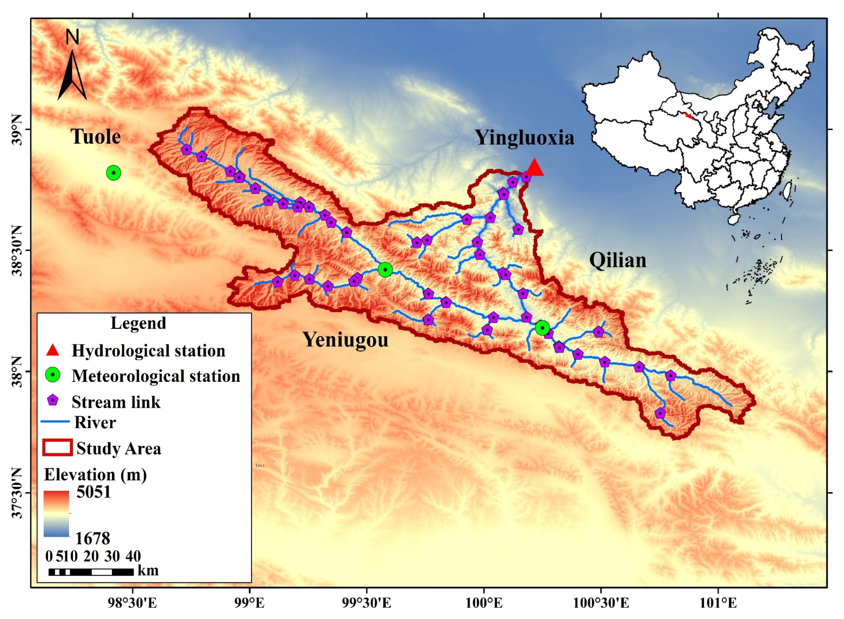
Figure 1. Location of the upper Heihe River basin.
Atmosphere 14 01083 g001
Figure 2. The framework of this study.
Atmosphere 14 01083 g002
Figure 3. The observed and simulated hydrographs derived from the SWAT model.
Atmosphere 14 01083 g003
Figure 4. The SWAT model simulation results for several high-flow processes during the calibration period (1990, 1996, and 1998) and the validation period (2003, 2008, and 2011). The black line is the measured value, the dotted line is the simulated value.
Atmosphere 14 01083 g004
Figure 5. Correction results for precipitation, maximum temperature, minimum temperature, relative humidity, wind speed, and solar radiation based on the EQM and LS methods.
Atmosphere 14 01083 g005
Figure 6. Projections of annual precipitation, maximum temperature, minimum temperature, relative humidity, wind speed, and solar radiation during future periods. The colored areas indicate the 10th to 90th percentile ranges of the projections.
Atmosphere 14 01083 g006
Figure 7. Differences in annual runoff in different future periods. An upward arrow indicates an increasing trend in future runoff compared to the historical period, while a downward arrow indicates the opposite.
Atmosphere 14 01083 g007
Figure 8. Differences in the seasonal runoff in different future periods. The horizontal line in the box plot represents the mean, and the square represents the median.
Atmosphere 14 01083 g008
Figure 9. Scatter plots of floods at different time scales for the two scenarios. The SSP245 scenario is pink, and the SSP585 scenario is blue.
Atmosphere 14 01083 g009
Figure 10. Flood projections for different return periods (the colored areas represent the 10th to 90th percentile ranges of the projections, and the solid line represents the projection of the MMEA).
Atmosphere 14 01083 g010
Figure 11. The timing of historical and future floods.
Atmosphere 14 01083 g011
Figure 12. Percentage of floods occurring in different months (May to October) during different periods. The SSP245 scenario is shown in blue, and the SSP585 scenario is shown in green.
Atmosphere 14 01083 g012
Figure 13. Differences in the summer precipitation (Pr), evapotranspiration (Et), and snowmelt (Mt) in the basin between the historical period and different future periods.
Atmosphere 14 01083 g013
Table 1. Details of the data source.
Data TypeData SourceResolution
Digital Elevation Modelhttps://www.gscloud.cn (accessed on
26 March 2021).
90 m
Land-use data in 2000https://www.resdc.cn/DOI/DOI.aspx?DOIID=54 (accessed on
19 April 2021).
1 km
Soil typehttp://www.fao.org/soils-portal/soil-survey/soil-maps-and-databases/harmonized-world-soil-database-v12/en/ (accessed on
19 April 2021)).
1 km
Table 2. Details of meteorological and hydrological data.
Type of StationsSite NameLongitude and LatitudeData Description
Meteorological stationsTuole98.42° E, 38.82° NDaily air pressure, wind speed, average temperature, maximum temperature, minimum temperature, relative humidity, precipitation, sunshine hours, with a time span of 1987–2014
Yeniugou99.58° E, 38.42° N
Qilian100.25° E, 38.18° N
Hydrological stationsYingluoxia100.18° E, 38.82° NDaily runoff data with a time span of 1987–2014
Table 3. List of GCMs used in this study.
Name of GCMCountryResolutionFrequency
ACCESS-CM2Australia1.875° × 1.25°daily
ACCESS-ESM1-5Australia1.875° × 1.25°daily
CanESM5Canadian2.8125° × 2.8125°daily
CMCC-ESM2Italy1.25° × 0.9375°daily
MIROC6Japan1.40625° × 1.40625°daily
MPI-ESM1-2-LRGermany1.875° × 1.875°daily
MRI-ESM2-0Japan1.125° × 1.125°daily
NorESM2-LMNorway2.5° × 1.875°daily
NorESM2-MMNorway1.25° × 0.9375°daily
TaiESMTaipei1.25° × 0.9375°daily
Table 4. Selection of parameters and their calibration results.
ParameterDescriptionRangeCalibration Results
v__SFTMP.bsnSnowfall temperature [−5, 5]4.6587
v__SMTMP.bsnSnow melt base temperature [−5, 5]3.2865
v__SURLAG.bsnSurface runoff lag time [1, 24]15.2123
v__ALPHA_BF.gwBaseflow alpha factor[0, 1]0.2937
r__CN2.mgtInitial SCS CN II value[−0.5, 0.5]0.1681
v__ESCO.hruSoil evaporation compensation factor[0.01, 1]0.3156
r__SOL_K.solThe soil layer’s available water capacity[−0.7, 0.7]0.5842
r__SOL_AWC.solSaturated hydraulic conductivity[−0.7, 0.7]0.6123
v__GWQMN.gwThreshold depth of water in the shallow aquifer required for return flow to occur[0, 5000]3046.6331
v__GW_REVAP.gwGroundwater “revap” coefficient[0.02, 0.2]0.0874
v__CH_K2.rteEffective hydraulic conductivity[0, 100]59.0481
v__CH_N2.rteManning’s nvalue for main channel[0, 0.3]0.2455
Table 5. Evaluation indicators in the calibration and validation periods.
PeriodR2NSEPBIASRSR
Calibration0.870.68−23.81%0.56
Validation0.890.71−26.31%0.54
Table 6. Mean absolute error of observed versus corrected daily data for the EQM and scaling methods (1987–2014).
GCMsMethodsPrecipitationMax.tempMix.tempHumidityWind SpeedRadiation
ACCESS-CM2Historical4.007.1113.310.281.275.61
Eqm1.604.093.880.141.123.87
LS1.624.694.540.111.164.67
ACCESS-ESM1-5Historical4.149.1918.220.331.215.37
Eqm1.644.093.890.131.123.88
LS1.594.554.250.101.094.64
CanESM5Historical3.918.4315.650.251.465.44
Eqm1.694.123.880.141.123.89
LS1.574.985.200.121.085.18
CMCC-ESM2Historical3.8610.0215.050.271.095.89
Eqm1.704.093.950.141.123.92
LS1.564.524.560.110.965.75
MIROC6Historical4.078.6516.230.271.465.80
Eqm1.594.093.940.141.123.97
LS1.684.364.060.111.065.61
MPI-ESM1-2-LRHistorical4.096.4213.590.342.316.44
Eqm1.684.193.950.141.123.95
LS1.634.764.690.111.095.64
MRI-ESM2-0Historical4.238.1115.160.231.815.76
Eqm1.594.173.990.141.133.85
LS1.644.764.770.131.015.37
NorESM2-LMHistorical3.7010.0016.510.221.515.54
Eqm1.664.103.880.141.113.88
LS1.584.684.490.130.995.47
NorESM2-MMHistorical3.7310.1515.900.211.435.49
Eqm1.644.093.880.141.113.89
LS1.604.764.500.131.005.39
TaiESM1Historical3.779.8913.650.241.106.31
Eqm1.664.234.020.141.123.98
LS1.584.805.200.130.966.32
Table 7. Trends in future floods and multi-year averages at different time scales under the two scenarios.
Time
Scale
SSP245SSP585
Trendp-ValueChange Rate (%)Trendp-ValueChange Rate (%)
1-day max0.12761.9%0.85566.4%
3-day max0.14134.3%0.74238.5%
5-day max0.15422.6%0.69426.2%
7-day max0.18818.7%0.57722.5%
Note: An upward arrow indicates an increasing trend in future flood compared to the historical period.
Table 8. Flood magnitudes in the historical period and the future for different return periods under two scenarios.
Time ScaleFuture Period30-Year Flood50-Year Flood80-Year Flood100-Year Flood
SSP245SSP585SSP245SSP585SSP245SSP585SSP245SSP585
1-day maxNF32.34%46.10%37.97%54.04%42.64%60.72%44.72%63.72%
MF16.45%39.01%20.03%44.97%24.31%52.16%24.31%52.16%
FF29.95%19.91%34.15%23.07%37.64%25.68%39.19%26.83%
Mean26.25%35.01%30.72%40.69%34.86%46.19%36.07%47.57%
3-day maxNF30.68%36.97%35.96%42.79%40.37%47.66%42.34%49.84%
MF12.39%32.98%15.30%37.98%17.71%42.16%18.79%44.02%
FF27.66%22.29%31.63%25.57%34.93%28.29%36.39%29.50%
Mean23.58%30.75%27.63%35.45%31.00%39.37%32.51%41.12%
5-day maxNF31.17%34.58%36.12%39.66%40.25%43.92%42.10%45.82%
MF11.38%32.23%13.78%36.74%15.77%40.49%16.66%42.16%
FF27.05%23.26%30.61%26.28%33.58%28.78%34.90%29.89%
Mean23.20%30.02%26.84%34.23%29.87%37.73%31.22%39.29%
7-day maxNF33.35%36.34%38.32%41.38%42.49%45.62%44.35%47.51%
MF14.41%35.67%16.88%40.32%18.94%44.20%19.86%45.93%
FF29.99%28.29%33.71%31.64%36.82%34.43%38.21%35.67%
Mean25.92%33.43%29.64%37.78%32.75%41.42%34.14%43.04%
Disclaimer/Publisher’s Note: The statements, opinions and data contained in all publications are solely those of the individual author(s) and contributor(s) and not of MDPI and/or the editor(s). MDPI and/or the editor(s) disclaim responsibility for any injury to people or property resulting from any ideas, methods, instructions or products referred to in the content.