Reconstructing PM_2.5 Data Record for the Kathmandu Valley Using a Machine Learning Model

Abstract

This paper presents a method for reconstructing the historical hourly concentrations of Particulate Matter 2.5 (PM_2.5) over the Kathmandu Valley from 1980 to the present. The method uses a machine learning model that is trained using PM_2.5 readings from the US Embassy (Phora Durbar) as a ground truth, and the meteorological data from the Modern-Era Retrospective Analysis for Research and Applications v2 (MERRA2) as input. The Extreme Gradient Boosting (XGBoost) model acquires a credible 10-fold cross-validation (CV) score of ~83.4%, an r2-score of ~84%, a Root Mean Square Error (RMSE) of ~15.82 µg/m³, and a Mean Absolute Error (MAE) of ~10.27 µg/m³. Further demonstrating the model’s applicability to years other than those for which truth values are unavailable, the multiple cross-tests with an unseen data set offered r2-scores for 2018, 2019, and 2020 ranging from 56% to 67%. The model-predicted data agree with true values and indicate that MERRA2 underestimates PM_2.5 over the region. It strongly agrees with ground-based evidence showing substantially higher mass concentrations in the dry pre- and post-monsoon seasons than in the monsoon months. It also shows a strong anti-correlation between PM_2.5 concentration and humidity. The results also demonstrate that none of the years fulfilled the annual mean air quality index (AQI) standards set by the World Health Organization (WHO).

1. Introduction

Air pollution poses a severe hazard to both the biotic (living organisms) and abiotic (hydrosphere, lithosphere, and atmosphere) components of our environment, as they are interconnected [1]. The rapid modernization of civilization, which encompasses increased traffic, construction, and industrialization, has had a significant impact on our air quality. The Particulate Matter 2.5 (PM_2.5) particles, with an aerodynamic diameter of less than 2.5 µm, make a substantial contribution to air pollution. Exposure to both smaller and larger airborne particles is detrimental, but PM_2.5 particulate matter directly contributes to cardiovascular and respiratory illnesses as well as mortality [2,3]. These particles can occasionally be toxic due to their chemical composition, which includes organic molecules, biological components, sulfate, nitrate, acid, and more [4].

The leading causes of high PM_2.5 concentrations in urban areas include rapid urbanization (construction), road dust, increased energy (fossil) consumption, and inefficient combustion [5]. On the other hand, major wildfires produce a significant amount of aerosols globally and some of them cause the formation of pyro-cumulonimbus (Pyrocbs) clouds [6], with some even reaching the stratosphere [7]. Pyrocbs are fire-triggered clouds of smoke. However, most of these wildfires contribute to surface aerosols and serve as sources of (PM_2.5) particles.

Nepal was among the ten nations with the worst air quality in the world in 2019, according to a report from the Health Effects Institute [8]. Nepal’s capital city, Kathmandu, is surrounded by other megacities with large population densities. Kathmandu has been identified as the most polluted city in Asia, according to Parajuly (2016) [9]. Temperature inversions caused by the unique mountainous environment of Kathmandu trap the polluted air. Pollution in Kathmandu includes the rising number of new and used diesel-engine vehicles, big trucks hauling sand and building supplies, deteriorating and unpaved roads, and hazardous metal operations on the streets near construction sites. Additionally, the extended disorganized rubbish management in open areas is a factor. Numerous brick-and-block production factories are dotted throughout the Kathmandu Valley’s three districts: Kathmandu, Bhaktapur, and Lalitpur, as well as on its outskirts [10]. The number of brick kilns in the Kathmandu Valley has increased by 200% and about 500 are in operation during the dry seasons [11]. These kilns contaminate the atmosphere by spewing smoke and dust [12].

The majority of people in Nepal follow the Hindu faith. A deceased person’s body is burned during cremation in the Hindu faith. In Nepal, open-air cremations are commonly performed, although electric indoor cremation has recently been practiced. The Pashupatinath temple, located on the bank of the Bagmati River in Kathmandu, is regarded as the holiest cremation site in Nepal. Kathmandu is a sacred city with several rivers of religious significance, including the Bagmati, Bishnumati, and others. Particulate matter (benzene, mercury, and polychlorinated dibenzodioxins and furans) is created during this process [13,14]. In light of this, Kathmandu’s PM_2.5 compositions are distinct from those of the rest of the world (except for some Indian cities). Overall, the PM_2.5 in Kathmandu is a unique and complex mixture of organic and inorganic materials.

Meteorological parameters along with precipitation are the major factors for the PM_2.5 concentration distribution and washouts [15,16,17]. The movement of PM_2.5 from emission sources to other places can also be impacted by the direction and speed of the wind. The mixing and vertical dispersion of pollutants, especially PM_2.5, can be influenced by temperature and air stability [18]. During steady atmospheric conditions (such as temperature inversions), pollutants frequently become trapped near the surface, leading to higher PM_2.5 concentrations. In contrast, unstable conditions promote vertical mixing and dispersion, which reduce PM_2.5 concentrations. PM_2.5 concentrations are not directly impacted by atmospheric pressure. However, variations in atmospheric pressure can have an impact on wind patterns, which in turn can affect how PM_2.5 is transported and dispersed. Therefore, existing sources, weather patterns, and geological characteristics all directly influence the occurrence of PM_2.5 [19]. Their dispersal is mainly influenced by wind and atmospheric stability [1,20]. Temperature, pressure, water vapor concentration, and other factors all affect the removal process, chemical production, and conversion of them. Thus, by identifying PM_2.5 precursors, we may increase our comprehension of the effects of PM_2.5 on several facets of life. A solid track record of air quality measurement is essential for pollution management plans. There have not been many long-term studies utilizing PM_2.5 to track the decadal trends in Nepal’s air quality. There are very few in situ measurement data available. Becker et al. (2021) and Mahapatra et al. (2019) list some earlier initiatives to detect air pollution in Kathmandu [21,22].

The Kathmandu Valley’s air quality was initially measured in the 1980s, however, seldom and only during specific seasons. The limited air quality measurements at the time included carbon monoxide, nitrous oxide, sulfur dioxide, and nitrous oxide. These investigations disclosed data on the initial pollutant concentrations and the seasonality of the valley’s air pollution [22]. The Nepalese government-built air quality monitoring stations at several locations throughout the valley between 2002 and 2007 to gauge particulate matter (PM₁₀ and PM_2.5) concentrations. Because the campaign was so short, no long-term trends could be drawn. Nonetheless, these campaigns showed that the air in urban (Kathmandu Valley) areas is two to four times more polluted than in rural areas [19,23].

Several other air pollution monitoring campaigns have been conducted over the years. From 2003 to 2005, the Ministry of Population and Environment (MOPE) conducted the first extensive monitoring campaigns on particulate air pollutants with the Danish International Development Agency’s (DANIDA) assistance. Nepal Health Research Council (NHRC) in the spring of 2014 [24] and a 2-week campaign in April 2015 [12] were among the critical PM_2.5-focused measurements. In the Kathmandu Valley, Black Carbon aerosol mass was measured for the first time in an urban environment between May 2009 and April 2010 [25]. At Paknajole, The International Centre for Integrated Mountain Development (ICIMOD) conducted measurements between February 2013 and January 2014. Since then, other large-scale, multi-country collaboration-based programs (including “Sus-Kat” and “NAMaSTE”) have been implemented to understand the various air quality-related concerns in Nepal [26,27,28].

Nonetheless, a reliable long-term record of air pollution over Kathmandu is still lacking, yet it is crucial for establishing patterns and conducting a social and health impact analysis. To address the issue, we offer a machine learning approach in this research to reconstruct the hourly PM_2.5 concentration in the Kathmandu Valley using available meteorological data. This work attempts to bridge the PM_2.5 data gap over Kathmandu. A long-term dataset with comprehensive meteorological parameters is needed as input to achieve this goal. Such datasets can be obtained from the Modern-Era Retrospective Analysis for Research and Applications-2 (MERRA-2) reanalysis data from the National Aeronautics and Space Administration (NASA) [29]. This study presents the reconstructed data record of the PM_2.5 mass concentrations in the Kathmandu Valley and examines its long-term climatology.

2. Data Sources and Pre-Processing

The US Embassy has set up an ambient air quality monitoring station in Phora Durbar (P.D.), Kathmandu (Latitude: 27.71° N, Longitude: 85.32° E), providing ground-based PM_2.5 data on an hourly basis since March 2017. In this study, we utilize these hourly PM_2.5 observations as the ground truth values for training the model. The data used for the analysis cover the period from March 2017 to March 2021.

MERRA2 is the atmospheric reanalysis data of the NASA Global Modeling and Assimilation Office [29]. It assimilated aerosol optical depth (AOD) data over the ocean from the Advanced Very High-Resolution Radiometer (AVHRR) from 1979 to 2002 [30]. Similarly, it assimilated the bias-corrected Moderate Resolution Imaging Spectroradiometer (MODIS) AOD from 2002 to the present [31], the Multiangle Imaging Spectro Radiometer (MISR) AOD from 2000 to 2014 (over the bright surface and desert only), and the AOD from ground-based Aerosol Robotic Network (AERONET) (1994 to 2014) [32,33,34,35]. The GOCART model is connected with the GOES atmospheric model to simulate mixed aerosols, including dust, sea salt, black carbon, organic carbon, and sulfate [29,36].

This study utilizes MERRA2 time-averaged hourly data for the Kathmandu Valley (Latitude: 27.5, Longitude: 85.625) from 1980 to 2021. The data used as input include surface pressure, total ozone column, wind speeds, temperature, and total precipitable water vapor. Additionally, the study incorporates information on the extinction, scattering, and mass concentrations of various aerosols, such as black carbon, dust, organic carbon, sulfate, sea salt, and aerosols. Specifically, the Dust Surface Mass Concentration (PM_2.5) is considered. In total, there are 28 variables as presented in

Table 1. MERRA2 time-average hourly input data for training the model include a list of meteorological data and a list of MERRA2 aerosol-related variables.

Meteorological data:
Total precipitable water vapor	Total column ozone	Specific humidity (2M)	Surface Pressure	10M Wind (U and V)	Temperature (2M)
Aerosols and dust species:
Surface Mass concentration	Extinction (O.D.)	Scattering (O. D.)	PM2.5 (Extinction)	PM2.5 (Mass)	PM2.5 (Scattering)
Dust	Dust	Dust	Dust	Dust	Dust
Organic Carbon	Organic Carbon	Organic Carbon	--	--	--
Sea salt	--	--	Sea salt	Sea salt	--
SO4	SO4	SO4	--	--	--
SO2	--	--	--	--	--
--	Total aerosol	--	--	--	--
DMS	--	--	--	--	--
Black carbon	Black carbon	Black carbon	--	--	--

that are included in the model for both training and prediction purposes. These variables collectively contribute to the model’s ability to analyze and make predictions.

The calculation of MERRA2 PM_2.5 is typically performed using Equation (1), as described in (https://gmao.gsfc.nasa.gov/reanalysis/MERRA-2/FAQ/#Q4, accessed on 10 December 2022) [32]. However, it should be noted that Equation (1) does not encompass the entire input list of PM_2.5. In order to address this limitation, a comprehensive comparison was conducted, taking into account both the PM_2.5 values predicted by the machine learning (ML) model and the values calculated using Equation (1). This comparison allowed for overcoming the constraints posed by the incomplete coverage of variables in Equation (1) and provided a more comprehensive analysis.

$${\mathrm{PM}}_{2.5}={\mathrm{Dust}}_{2.5}+{\mathrm{SS}}_{2.5}+\mathrm{BC}+1.6\times \mathrm{OC}+1.375\times \mathrm{Sulfate}$$

(1)

In Equation (1), Dust_2.5 is the Dust Surface Mass Concentration of dust (with radii < 2.5 µm). The above equation considers the surface mass concentration of dust PM_2.5, sea salt_2.5, black carbon, and sulfate. Still, it does not account for nitrate emissions (primarily produced by industrial processes and vehicle exhaust), ammonium, silicon, sodium ions, elemental carbons, etc. [29]. A study in China shows that the absence of those elements results in a significant underestimation of PM_2.5 retrievals. [15]. Such discrepancies can be verified with trustworthy ground-based measurements, and the long-term bias-corrected data records would be strengthened and supported by simulating the rectified PM_2.5 data.

The distribution of PM_2.5 is significantly affected by many factors, such as meteorological parameters, surface conditions, pollutant emissions, and population distributions [37]. In our ML model, population distribution is not included as a factor. This is primarily due to the unavailability of a reliable, long-term source of population data that can be consistently incorporated into the model. Estimating the missing PM_2.5 components is made possible by comparing the hourly proportion/variation of meteorological variables from MERRA2 with the variation in the PM_2.5 precursors that are already accessible. The MERRA2 variables can be related to the missing components in the total mass of PM_2.5 and used to offset it partially. For example, the entire ozone column, coupled with the temperature and pressure, all imply a certain concentration of nitrous. Many studies have shown that the NOx concentration directly correlates with the morning formation and evening–night breakdown rates of ozone as well as the variance of volatile organic compounds (VOCs) [38,39]. The shift in temperature, longwave (terrestrial), and shortwave (solar) radiation intensities throughout the day cause such variations. Among VOCs, organic carbon represents a portion of it. Hence, the missing proportion, primarily caused by the nitrate concentration in the local PM_2.5, can be reduced by integrating ozone data with metrological factors. The application of machine learning can significantly improve the situation, as demonstrated by the metrics analysis of the model in the test data in the Results section. Table 1 gives a list of factors from MERRA2 that are used for the PM_2.5 data record reconstruction.

Although it is conceivable that not every variable we picked directly causes or contributes to PM_2.5, their oscillation and fluctuation with other variables suggest and aid in estimating PM_2.5. By building a suitable model, machine learning excels at assessing and characterizing the distinctions between them.

3. Machine Learning

Machine learning is potentially a helpful method for capturing the complex inter/intra play of selected variables with the target values. The US Embassy at Phora Durbar has continuous ground-based PM_2.5 data going back almost five years, which can serve as the truth for training the machine learning model. A machine learning algorithm makes predictions by mapping input features to a single output based on the relationship between input and truth values (regression or classification). The missing components of Equation (1) have a combined influence on the surface PM_2.5 mass concentration, as was mentioned in the previous section. Potentially relevant MERRA2 meteorological variables include local temperature, pressure, relative humidity, wind speed and direction [40,41,42], total ozone columns, and various aerosol extinction and optical depths. All of these elements interact, and that interaction can significantly impact how much PM_2.5 is present and distributed in the area [17,43]. With MERRA2 meteorological and environmental data as input features (Table 1) and Phora Durbar ground-based PM_2.5 mass concentration as a truth value, we are better equipped to apply and evaluate various Machine Learning models.

There are numerous types of machine learning regression models. To select the best model for this study, we chose to compare the following models: Linear Regression (L.R.), Decision Tree (D.T.), Random Forest (R.F.), and Extreme Gradient Boosting (XGBoosting (X.G.)). The common theme of these methods is to train the model to find the best prediction by minimizing the errors between the output and the input “truth.” The L.R. approach looks for the best fit using multi-linear regression; the D.T. method establishes regression using a tree structure. The model reaches the final results using decision nodes and leaf nodes. The R.F. technique uses multiple independent decision trees to predict a response given a set of predictors. The algorithm then merges the outcomes by averaging the final outcomes. The X.G. method is also a decision tree ensemble algorithm, similar to the R.F. methods in this regard. The difference is that the X.G. method improves a single weak model by combining it with other weak models. It does that through iteratively training a new model using the error residual of the previous model. In other words, the R.F. method generates decision trees in parallel, while the X.G. is a sequential model, where each subsequent tree is dependent on the last one. More details about X.G. will be given later in this section.

The statistical metric R squared (r2-score) value is used to assess the fitness of a regression model. While using 28 input features in Table 1, the performances of each of these models are contrasted in terms of their cross-validation score, r2-score, Mean Absolute Error (MAE), and Root Mean Squared Error (RMSE). Such metrics are calculated as follows:

$$r_2\left(score\right)=1-\frac{Residual Sum of Squared Error}{Total Sum of Squared Errors}=1-\frac{{{\displaystyle \sum }}_{i=1}^N {\left(y_i-y_{pred}\right)}^2}{{{\displaystyle \sum }}_{i=1}^N {\left(y_i-y_{mean}\right)}^2}$$

(2)

$$Root Mean Square Error \left(RMSE\right)=\sqrt{{{\displaystyle \sum }}_{i=1}^N\frac{{\left(y_i-y_{pred}\right)}^2}{N}}$$

(3)

$$Mean Absolute Error\left(MAE\right)={{\displaystyle \sum }}_{i=1}^N\frac{\left|y_i-y_{pred}\right|}{N}$$

(4)

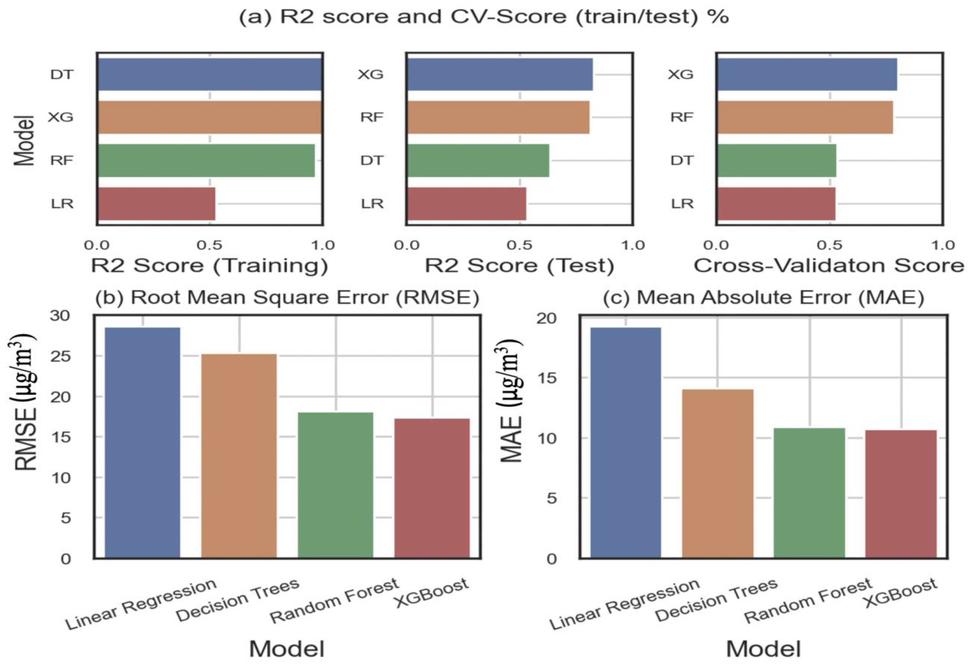
where y_i, y_pred, and y_mean are the ith measurement; the model predicted value, and the mean of truth value, respectively, where N is the total number of samples. Figure 1a demonstrates that the X.G. algorithm has the highest r2-score and Cross-validation score. The lowest MAE and RMSE figures are also produced by X.G. (Figure 1b,c). The most notable regression overall is the X.G. one. In contrast to R.F., which is vulnerable to overfitting in noisy data, it has also been demonstrated that the X.G. efficiently prevents overfitting and minimizes computing complexity [44]. We decided to use the X.G. regression method in light of this.

The collection of serialized decision trees that cooperate to finish a task is at the core of the XGBoost ML. It is superior because it considers the contribution of each tree before building a serial model that incorporates every variable.

The XGBoost algorithm, a gradient-boosted (trees are serialized to reduce the loss function in subsequent trees) decision tree technique, was first introduced by Chen and Guestrin (2016) [45]. Since then, there has been constant growth and progress. Recently, the XGBoost, a scalable machine learning technique that outperforms several widely used existing classifiers and uses tree boosting to prevent overfitting, has caught the attention of researchers. Its multiprocessing algorithm can process massive amounts of data.

Boosting is a group learning method in which weak learners are united to produce strong learners to work together to reduce training errors and boost the model’s performance. Even when random forests fit trees that depend on one another to lessen the bias of the strong learner, boosting is often more effective than bagging. Gradient boosting (G.B.), a sequential training method, devalues models that have previously been incorrectly classified. By parallelizing the training procedure, Extreme Gradient Boosting (XGBoost) improves computational speed while utilizing multiple cores [45].

The base model is first created, which yields outputs for each instance, and then the residue (prediction error) is obtained. A further model is trained to fix the previous error, obtaining a new, improved gain value and an improved model. It continues in sequence until all true values are correctly trained, or a defined number of trees are reached, with the largest gain for each tree. In this way, several models are created with multiple gain values.

The major steps of the XGBoost model are expressed in the summary equations, as explained by Chen and Guestrin (2016) [45]:

First, the model assumes the base model, as shown in Equation (5). For a given dataset having $n$ examples and $m$ features, a tree ensemble model uses $K$ additive functions to predict the output:

$$\widehat{y_i}=\phi \left(x_i\right)={\displaystyle \sum }_{k=1}^K{f}_k\left(x_i\right)$$

(5)

where the symbols are $\widehat{y_i}$= Model predicted PM_2.5, $x_i$= the vector representation of 28 input variables and $f_k$ is an independent tree and contains a continuous score on each leaf. Based on the predicted value from Equation (5), a model is trained in an additive manner. As the equation describes, a new tree is created to minimize the error (objective) observed during the previous base model, as expressed by (5). Scores of corresponding leaves sum up the final model prediction. The objective function used to train the model is a sum of a differentiable loss function and a regularization term. So, to learn the set of models, the regularized objective function term is minimized as:

$${\mathcal{L}}^t={\displaystyle \sum }_{i=1}^n\mathcal{l}\left(y_i,{\widehat{y}}_i^{\left(t-1\right)}+f_t\left(x_i\right)\right)+\mathrm{Regularization} \mathrm{term}$$

(6)

.

In Equation (6), $\mathcal{l}$ is a training loss function that expresses the relation between the truth ($y_i$) and the predicted value ${\widehat{y}}_i^t$. The common way to evaluate it is using the Mean Squared Error (MSE). Similarly, ${\widehat{y}}_i^{\left(t-1\right)}+f_t\left(x_i\right)$ is predicted at iteration t−1. The addition of each new $f_t$ balances the error in each iteration. The ‘Regularization term’ in XGBoost is influenced by both the learning rate and the minimum child weight. Additionally, it is dependent on the number of leaf nodes in a tree and the weights assigned to those leaves. Using a gradient boosting approach, the XGBoost algorithm minimizes this objective function (shown in Equation (6)). Each decision tree in the ensemble is trained to minimize the negative gradient of the objective function with respect to the predicted values. The final prediction is the weighted sum of the predictions of all the trees in the ensemble [45]. So, instead of using the average of each tree to forecast the final model output values, one can learn from past mistakes and develop a robust model.

4. Methodology

To build the desired machine learning model, we start with coupling the P.D. PM_2.5 data (truth value) to the MERRA2 data (input variables) for the time within a 15-min window. With the 28 features in Table 1 as input, the algorithm was tested and trained using data from March 2017 to March 2021. Note that this period covers a wide range of PM_2.5 situations. For example, in 2020, several primary human sources of PM_2.5 were substantially lower compared to other years due to the COVID-19 lockdowns.

As the next step, all the data are randomly divided into two groups: 20% is set aside for testing and 80% is used to train the model (80/20% split). The X.G. Model’s numerous hyperparameters are tweaked and tested to choose the ideal combination of input variables and hyperparameters using the ‘Randomized Search’ 10-fold cross-validation scores. Those parameters and their contributions [45,46] are listed below in

Table 2. XGBoost Regression Model’s selected tuned hyperparameters and their short description.

Hyperparameters	Description
Eta (learning rate)	Controls the step size at each iteration while updating the weights of a decision tree by preventing overfitting and generalization.
n_estimator	Number of decision trees to be built. The larger number of trees makes the model more complex and better but may lead to overfitting.
max_depth	Maximum depth of each decision tree. Higher values allow more splits and capture the complex interaction between each feature.
min_child_weight	Determines the thresholds on the sample to split.
subsample	It is the fraction of samples to be randomly sampled for each tree in the ensemble.
colsample_bytree	Fraction of each tree’s features also helps prevent overfitting.
objective	Specifies the loss function to be optimized during training.

:

The results of such pairings are noted in testing data using the r2-score. In testing data, the r2-score ranged from ~64% to ~84% for various combinations of hyperparameters. So, a good variety of properly hyperparameter-tuned models significantly improves the model’s performance. The base model to be deployed is 84%. At first glance, some of the 28 listed criteria appear to be only distantly related to PM_2.5. However, combining them will yield the optimal metrics for the model. So, even if their bulk has no direct impact on the PM_2.5, their interaction with other variables does. Examples include temperature, pressure, etc., which are not PM_2.5 components but suggest the PM_2.5 mass variation scenario. In this case, ML is helpful in capturing the variances.

Figure 2 displays the feature ratings of the input variables for the XGBoost’s default importance for the top 10 variables. The meteorological environment affects air quality and PM_2.5 levels. The specific humidity seems to play the most prominent role in forecasting the PM_2.5 concentration in the Kathmandu Valley. Various sources of PM_2.5, such as incomplete combustion, forest fires, dust, etc., rank lower compared to other input components regarding their relative significance. In Section 4, we further explore its relationship to the PM_2.5 levels. These rankings demonstrate that when estimating PM_2.5 levels, meteorological parameters are more crucial in identifying the actual contributors. As a result, we can rely on the model to take into account some of the missing PM_2.5 contributors that are not easily accessible to us in explicit forms, such as the various nitrate compounds, but are well suggested by meteorological data in its implicit form and will be handled by the model in the proper proportions. However, the most accurate way to assess a model’s performance is to test it against data that it has never seen before.

5. Results

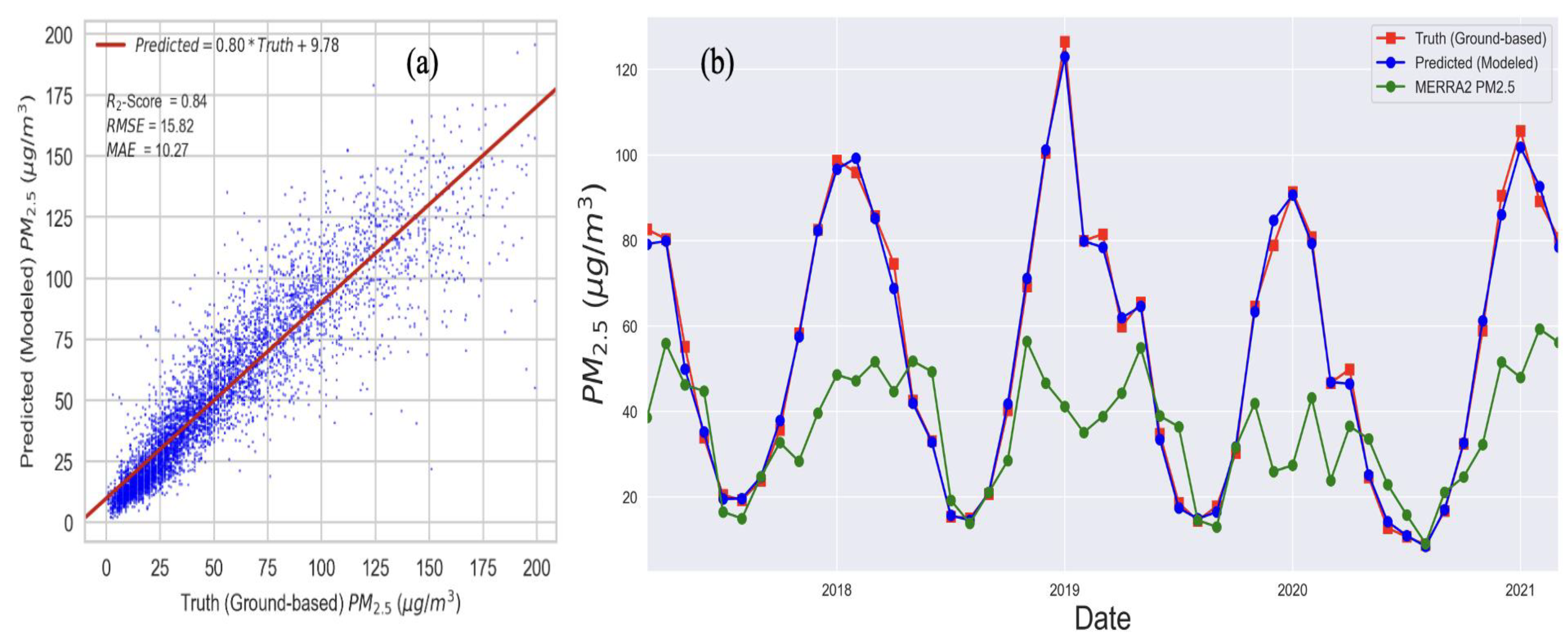
The trained model, which was developed using 80% of the data, is then applied to the remaining 20% of the randomly selected unused data from the period spanning 2017 to 2021. The relation between the actual PM_2.5 mass concentration and the model-predicted PM_2.5 mass concentration is depicted in Figure 3a. The mean absolute error is 10.27 µg/m³, the root mean square error is 15.82 µg/m³, the mean difference is 0.4 µg/m³, and the coefficient of determination between the projected value and the actual value is 84%. It is also revealed that nearly one-third of PM_2.5 concentrations are greater than 100 µg/m³, which is a health-frightening amount.

The monthly average time series for the same 20% tested, truth values, and MERRA2 PM_2.5 are displayed in Figure 3b. With the 84% coefficient of determination, we anticipate a higher degree of agreement between the truth and the predicted values. Here, averaging them over a month reveals a nearly perfect match, indicating its applicability to climatology and long-term trend monitoring. MERRA2 PM_2.5 displays a similar seasonal pattern in months with low-mass concentrations and a better correlation with actual data and predictions. When high PM_2.5 concentrations are present, MERRA2 significantly biases low. This comparison demonstrates that the MERRA2 does not sufficiently account for the emission of particles in its computations, which was previously discussed in this paper and in the work by Jin et al. (2022) [15]. Long-term climatology investigations and data creation are sparked by the frequent low-bias MERRA2 representations in various studies and the literature mentioned above, which motivates more research and model use. Figure 3b also illustrates the seasonality in the readings of PM_2.5 over Kathmandu. Higher concentrations sustain the periodicity near the end and beginning of the year, while dropping concentrations support it in the middle.

It has been shown that ML development works quite well with split samplings of 80%/20% [47]. Yet, because aerosol concentrations involve complex factors that are constantly changing, we should proceed with caution before pronouncing such a model to be the best. Even while we think that a 20% random sample of the data correctly captures the distribution of the data, there are times when testing data is entirely new, such as when selecting a different year, the ML metrics start to decline. We must, thus, conduct several tests in various scenarios based on earlier predictions that have been proven valid scientifically to construct a usable model. Truth values from 2017 to 2021 also consider that multiple COVID-19 lockdowns in 2020 resulted in a very different PM_2.5 period, as mentioned before. In terms of pollution brought on by human activity, such as the significantly decreased usage of vehicles, almost closed kilns, the restricted amount of construction, etc., it is akin to the early 1980s and the 1990s. As a result, it provides the leverage needed to determine whether the model can accurately predict occurrences, such as those in the 1980s and 1990s. To test the validity of this machine learning approach, we purposely left out the data from the year to be assessed when training the model. For example, for the 2018 testing, we used data from 2017 and from 2019 to 2021 to train the model and left out the entire 2018 data as unobserved data to test the model. We used the same strategy in 2019 and 2020. Not having data for all 12 months, 2017 and 2021 are not assessed with this method. This alternative testing methodology does not use an 80/20 split. In this instance, the testing data distribution is entirely new and unseen for the model, which may not be the case for splits of 80/20 %.

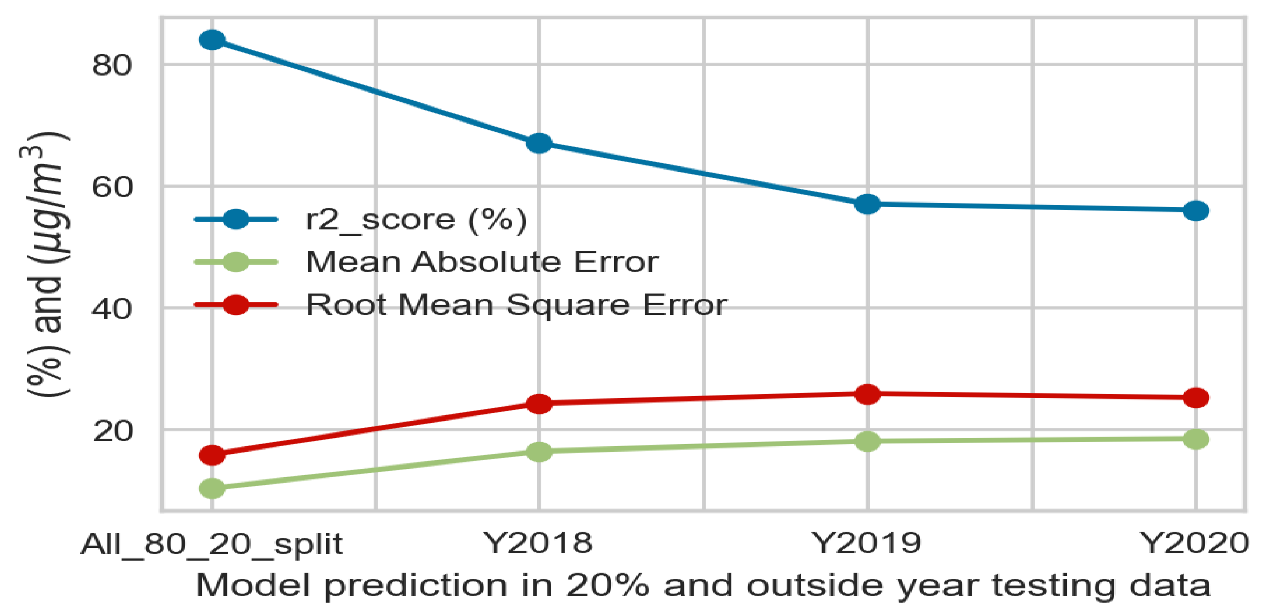
The full metrics analysis of all these tests is shown in Figure 4. As seen from the figure, compared to the metrics derived using the 80/20% split, the r2-score decreased, and the MAE and RMSE increased. For example, the r2-score is 67% for the 2018 testing, the MAE is 16.35 µg/m³, and RMSE is 24.23 µg/m³, while the corresponding values when using the 80/20% split are 84%, 10.27 µg/m³, and 15.82 µg/m³, respectively. This is expected because, for the 80/20% split, data from all years are sampled; the test data likely share the same distribution as the training data since they are from the same years. When the entire year is used for testing, the data distribution patterns can differ from the training dataset. In this regard, the test result for the year 2020 is especially suited for evaluating the model’s performance because the aerosol data patterns can be very different due to the pandemic lockdowns. However, the model still performed well, with an r2-score of 56%, an MAE of 18.52, and an RMSE of 25.3 µg/m³.

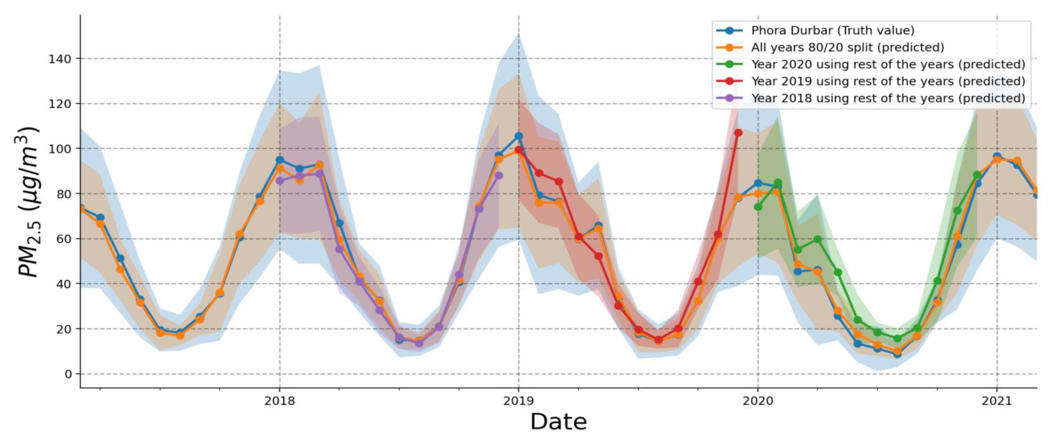
The monthly averages from the various cross-tests are shown in Figure 5, along with the truth values. Each hue represents the PM_2.5 concentration anticipated by the model for each particular year with a shaded standard deviation. It also contains the projected 80/20% split test results, which match a truth value. The remaining test data for each year using the model trained for the remaining year demonstrate good agreement in comparing true monthly averages. If we perform an hour-by-hour examination, the disparity between all projected concentrations and the actual values is more prominent. However, for a trend and seasonal comparison, the repeated cross-tests of the model yield a solid estimate.

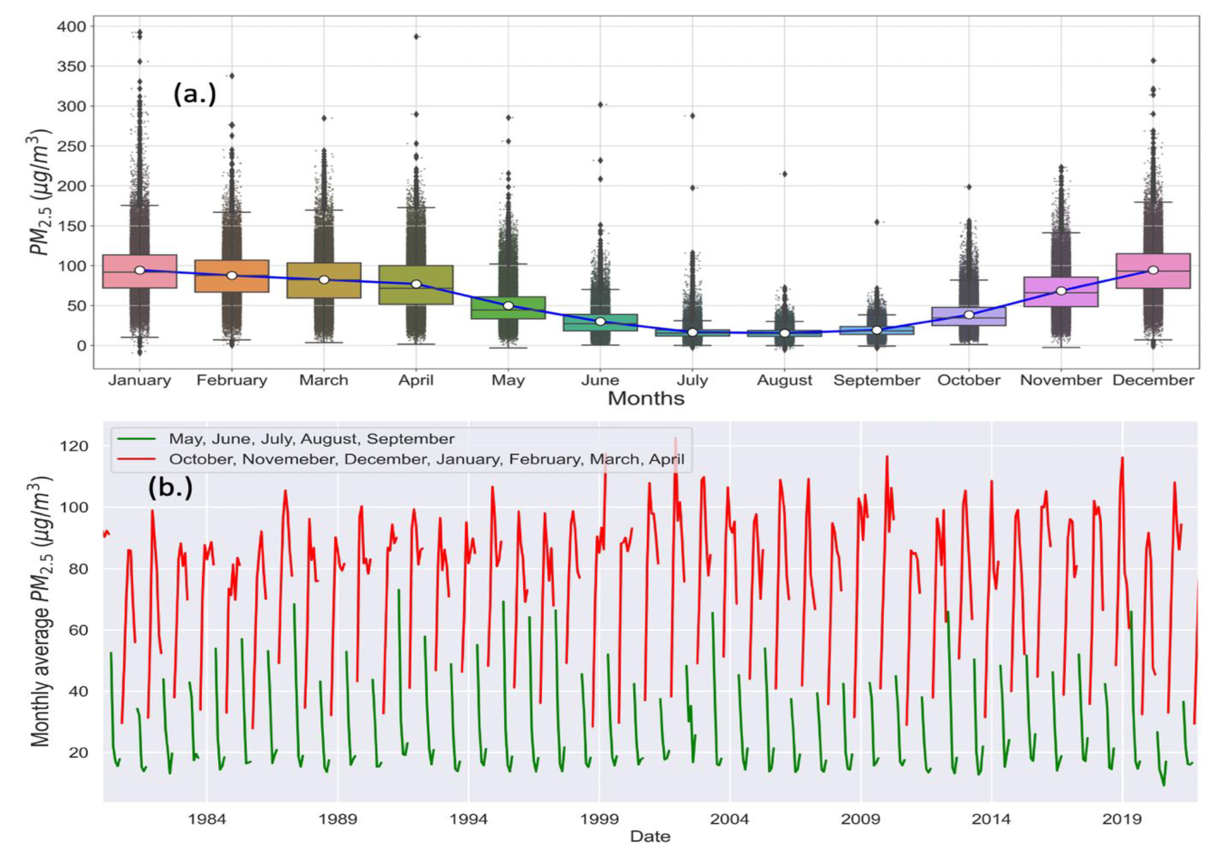
We anticipated a wealth of information to be available for the analysis and research into the climatology and history of PM_2.5 by looking at the long-term data record. We used the trained model to reconstruct the hourly PM_2.5 data from 1980 to 2021. Figure 6a represents the monthly distribution of PM_2.5 during all years. It further confirms the seasonality of PM_2.5, established in testing the data, over a lengthy period. Based on the distribution of PM_2.5 mass, there are primarily two seasonal patterns: rainy and non-rainy. Along with the dynamics and chemistry of the various elements, human-made effects also contribute to seasonal variance, but local weather phenomena play a vital role.

The rainy (monsoon) season typically lasts roughly from June to September in Kathmandu, Nepal [48]. We included May also in this season, which is full of rainy days, some of which might linger for several days and can occasionally result in life-threatening flooding. We noticed that the PM_2.5 concentration dropped low starting in May. The PM_2.5 concentration was at its lowest point of the year when the rainy season peaked in July and August, with a mean value of 25 µg/m³ and a reasonably small interquartile range, as shown in Figure 6a,b. Figure 7a demonstrates that the distribution of PM_2.5 during monsoon months is more concentrated around mean and median values, with a condensed interquartile range. It aids in calculating the Inter Quartile Range (IQR), or the difference between Q₃ (upper) and Q₁ (lower) quartiles. Analyzing how compact the data distribution is can be helpful too. Two whisker caps up and down, commonly called the outlier threshold, similarly represent the specified maximum and minimum values gathered by the Q₃ + 1.5 × IQR and Q₁ − 1.5 × IQR (in this case). Since these occurrences do not always match the distribution of most data from the same groups, they are called outliers. However, here, they represent some high-concentration events of PM_2.5 rather than outliers. Consequently, taking these into account in subsequent calculations depends on the purpose, result, and impact of these data.

Building and brick manufacturing stoppages and frequent rain-related washouts are among the factors that cause PM_2.5 levels to drop during monsoon seasons. On the other hand, pre- and post-monsoon months greatly vary from the median and mean with considerable expansions of many points above 75% and frequently exceeding 175 µg/m³ to show a significant enhancement of PM_2.5 in these seasons.

Figure 6b compares the monthly mean PM_2.5 between the dry and rainy seasons. The air quality (PM_2.5) in Kathmandu is at its healthiest during the rainy months, albeit not meeting World Health Organization (WHO) standards of the Air Quality Index (AQI), as shown in Figure 6b. According to the WHO, the yearly mean PM_2.5 AQI for healthy air is 10 µg/m³ and the 24-h daily average is 25 µg/m³ [49]. It clearly distinguishes between the monthly average of PM_2.5 for rainy and dry months. For the dry months, the construction (big buildings, houses, roads, etc.) process picks up significantly, the brick factories begin to reopen, there is less rain to wash the dust away, and the lack of moisture causes the muddy roadways to turn dusty. Due to the landscape of the Kathmandu Valley, a temperature inversion can easily develop during the cold season, retaining pollution until there is strong wind assistance or rain washout. As a result, high concentrations are shown to endure. As per these models’ predicted data, the average number of healthy days in Kathmandu from 1980 to 2021 was just 160. It shows how seriously polluted air is in the Kathmandu Valley.

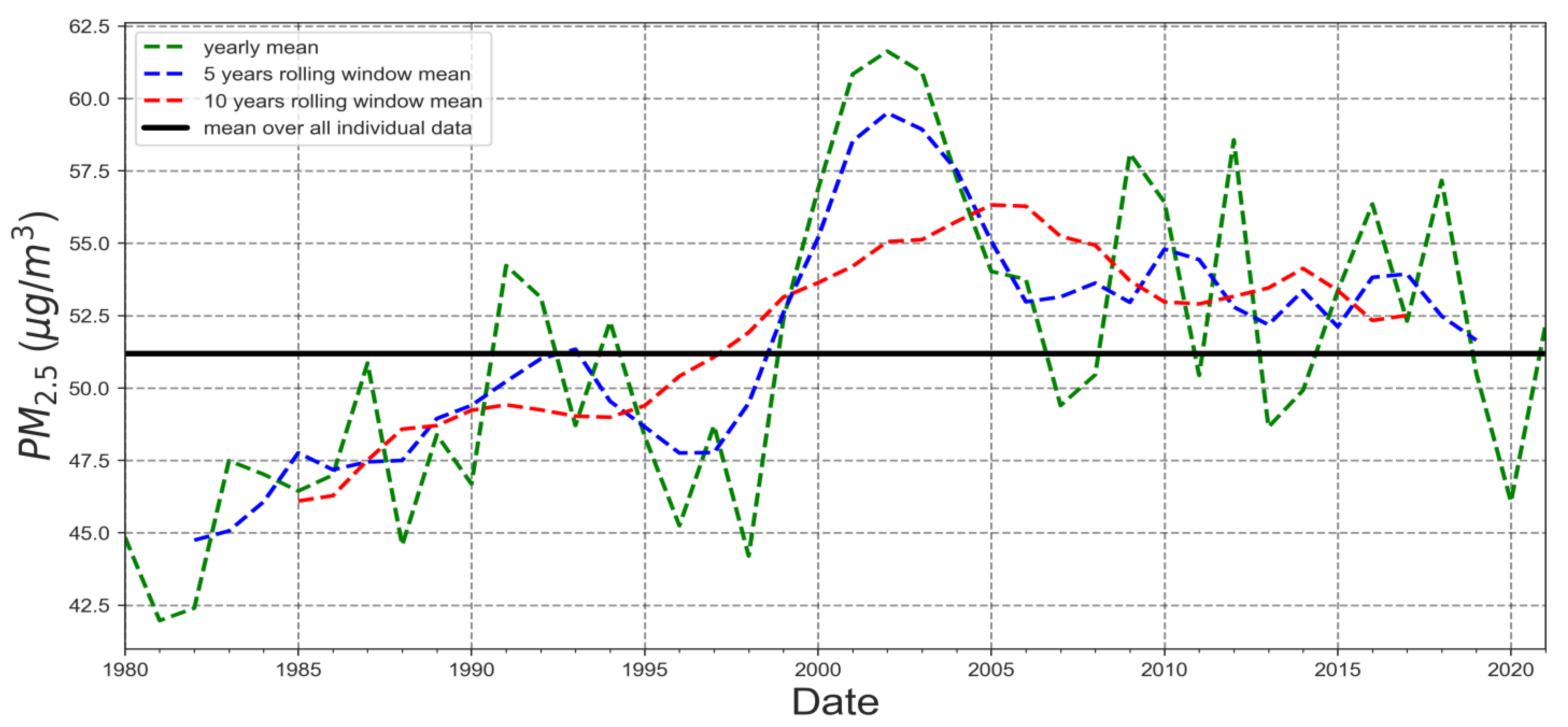
The decadal rolling average of that statistic shows an increase in the PM_2.5 concentration from 1980 to 2005. As shown in Figure 7, the annual average has some ups and downs, but the concentration does increase consistently until 2002. The years 2001 and 2002 appear to have had the highest PM_2.5 levels. This is also accurately reflected in the five-year rolling average. By combining yearly, half-decadal, and decadal averages, it was possible to summarize the distribution trend throughout the Kathmandu Valley, which had been rising until 2002 before beginning to modestly decline and demonstrating a steady concentration of decadal average PM_2.5 concentrations after that. Figure 7 displays the mean of all individuals as a horizontal black baseline, with a concentration of 51.19 µg/m³. The rolling decadal average continuously climbs from 1980 to 2005, with a slight decline. However, specific years exhibit a modest deviation from the mean on occasion. Due to COVID-19 lockdowns, as discussed earlier, 2020 brings a concentration level much lower than typical, which is well demonstrated by the model.

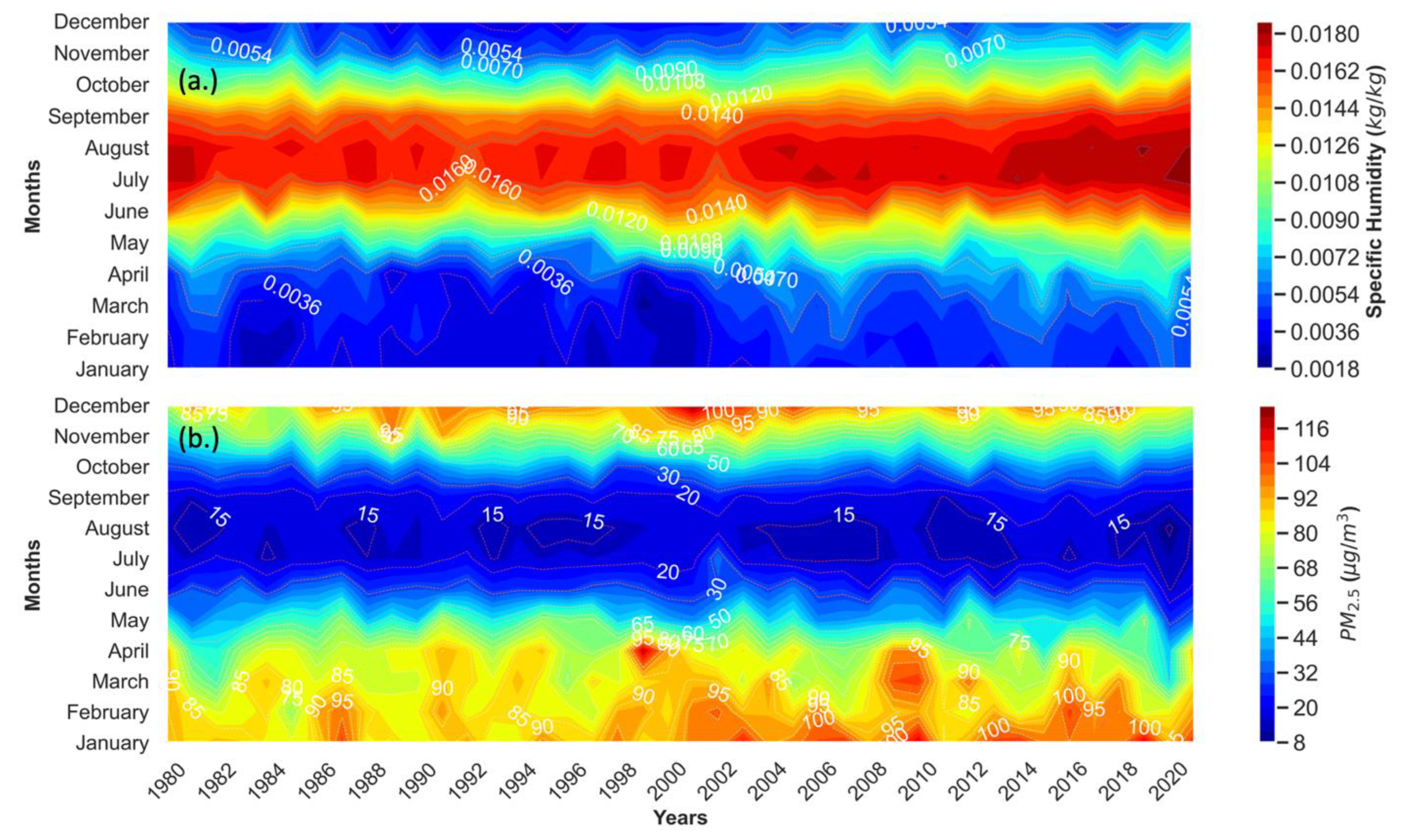
The two most important input factors that influence the model’s predictions are specific humidity and the total amount of water vapor that can precipitate. Figure 8a,b illustrate the strong anti-correlation of PM_2.5 with specific humidity. The big blue band in Figure 8b indicates the middle of the year monsoon months, generally from May to September, with a lower PM_2.5 mass concentration than the other months. Compared to the monsoon months, other months have greater PM_2.5 concentrations. Figure 8a shows a distribution of lower specific humidity during the months with higher PM_2.5 concentrations shown in Figure 8b, which is precisely the opposite distribution in Figure 8a,b. It suggests that PM_2.5 levels in the Kathmandu Valley are lower during extremely humid seasons and vice versa. This conclusion aligns with Liu et al. (2020) [50]. High humidity is a manifestation of rainy weather, which washes out aerosols. In addition, hygroscopic growth at times of high humidity makes the aerosol particles (PM_2.5) heavier and causes them to fall by dry deposition [51]. As a result, PM_2.5 concentrations are reduced. In addition, Wang et al. (2013) conducted a thorough analysis of Beijing, China, to look at the contribution of meteorological factors to PM_2.5. Beijing’s typically dry, chilly winter has greater PM_2.5 levels than the muggy, hot, rainy summer [52]. As expected, similar results were achieved in the projected model and actual PM_2.5 concentrations over the Kathmandu Valley confirming the rationality of the model’s performance.

6. Summary

The concentration of PM_2.5 is predicted using various machine learning regression models. These models were created and assessed for approximately five years, from March 2017 to March 2021, using surface level MERRA2 time average meteorological and aerosol parameters as input features and Phora Durbar PM_2.5 mass concentration data for training. This work generated long-term historical PM_2.5 concentrations in the Kathmandu Valley, a metropolis with a high population density. With a high r2-score of almost 84% and a low root mean square of 15.82 µg/m³, the XGBoost machine learning model stands out among the various regression models. In multi-cross tests, it succeeds, demonstrating that the statistics produced are satisfactory for the specified study. The trained model is used to reconstruct the long-term PM_2.5 mass concentrations in the Kathmandu Valley beginning in 1980. The primary contribution of this research is a viable approach to close the data gap for PM_2.5 in the climatological study of the Kathmandu Valley.

Analysis of the reconstructed PM_2.5 time series shows that only around 160 days from 1980 to 2021 fulfill the WHO’s AQI of PM_2.5 requirements. It highlights the significant health risks that the Valley’s PM_2.5 presents. Both ground-based data and machine learning forecasts support the seasonal trend of the Kathmandu Valley’s PM_2.5. This study demonstrates increased trends in PM_2.5 from the 1980s to 2002. After 2002, it begins to decrease slightly. The result also shows clearly the COVID-19 lockdowns’ influence on lowering PM_2.5 in 2020 in terms of annual mass concentration.

This approach appears to be effective at reconstructing long-term PM_2.5 levels. The applicability of the model can be expanded by considering new locations and truth values. By including additional years’ worth of future true value, the accuracy of this model can be further improved. This study’s practical application is to offer a framework for rebuilding PM_2.5 data records in areas without comprehensive historical data. Based on the connections with meteorological factors, we may fill in missing PM_2.5 data using machine learning models. This reconstructed dataset can be used for a number of tasks, including analyzing trends in air quality, carrying out epidemiological research, and assisting with the formulation of air pollution mitigation legislation.