1. Introduction
Atmospheric visibility is the maximum horizontal distance at which a person with normal vision can see and recognize the outline of a target object from the sky background. The use of various solid fuels emits large amounts of sulfur dioxide and other particulate matter into the air, as well as exhaust emissions from moving vehicles, all of which directly contribute to reduced atmospheric visibility [
1].
Many scholars have conducted much research on visibility in recent years. Liu et al. [
2] proposed a depth-integrated model and achieved good performance in a variety of well-known experiments, especially in the classification of visibility differences. They used this model and multiple nonlinear regression analysis to discuss the visibility classification and influencing factors at an airport and found that visibility was significantly correlated with relative humidity, temperature, and the mean wind speed. Peng et al. [
3] proposed an improved visibility parameterization: the direct extinction coefficient of fog droplets, and an overall improvement in the low-visibility simulations for the whole Beijing-Tianjin-Hebei region was achieved using the improved parameterization, with a significant reduction in error. The simulation results show that the decrease in visibility is closely related to the increase in aerosol particle mass concentration and the increase in relative humidity. Zhang et al. [
4] adjusted the atmospheric visibility observations from 582 stations across China to eliminate or reduce the effects of changes in the observing system. Based on the annual average visibility series of the adjusted data, the relationship be-tween visibility and wind speed from near the ground to the troposphere was analyzed, and the results showed that the "maximum" ("minimum") visibility corresponds to the "maximum" ("minimum") wind speed near the ground and in the lower troposphere. Xue et al. [
5] used a long-term continuous humidification turbidimeter system to measure multi-wavelength aerosol scattering coefficients under dry conditions and controlled relative humidity in spring and summer in the North China Plain, revealing a nonlinear relationship between visibility and PM2.5 mass and encouraging further research by future generations. Ting et al. [
6] proposed one-year continuous measurement data from an integrated online instrument to study the seasonal effects of aerosol chemistry in PM2.5 on visibility, addressing the shortcoming that long-term and in situ measurements of atmospheric particle chemistry were not available in most previous studies. Zhang et al. [
7] developed a logistic regression model between low visibility and wind speed, and the results showed that visibility improved with an increasing wind speed, which confirmed the effect of air pollution control in China since 2013, with both deterioration and improvement of air quality over time. Unlike traditional studies that focus on temporal variability of aerosol properties under average conditions, Li et al. [
8] investigated the long-term trends in extreme surface aerosol extinction coefficients in China using visibility datasets and found that interdecadal variability of pollution in China may be governed by different mechanisms and that weather conditions leading to extreme air quality changes may have dominated in the 1980s.
Most scholars have studied the effects of aerosols and various meteorological factors on visibility variation from data in the time domain using various methods and have achieved many excellent results, but there is a lack of research on the time-frequency domain variation in visibility data itself. The time-frequency domain analysis method has been applied in many fields; Magazzino et al. [
9] used wavelet analysis studies to discover the causal relationship between energy consumption and economic growth at different time scales and frequency bands using datasets, such as energy from Italy for more than eighty years, justifying the decomposition of the time series into various time scales using wavelet transform. Meng et al. [
10] used different scales of discrete wavelet transform (DWT) to decompose and reconstruct the original reflectance (OR) and first-order derivative reflectance (FDR) at different scales, which solved the problem of the difficulty in mapping the spatial distribution of soil organic carbon (SOC) in most studies, and the DWT combined with some prediction algorithms significantly improved the prediction accuracy of SOC. Li et al. [
11] used continuous wavelet transform and other methods to portray the connection between meteorological drought and hydrological drought in a specific time domain, which is important for promoting early warning and the mitigation of hydrological drought. Almounajjed et al. [
12] used the raw asynchronous motor current obtained by continuous wavelet transform (CWT) analysis in the time domain to precisely specify the number of short-circuit turns in the defective phase of the asynchronous motor, and several experimental results proved the practicality, effectiveness, and high correctness of the method. This paper applies the time-frequency domain combined analysis method to the long-term changes in visibility in China and analyzes the specific changes in visibility in the frequency domain.
Visibility is closely related to people’s lives, and poor visibility can have adverse effects on people’s lives, such as highway congestion and aircraft departure delays, so the prediction of future trends in visibility has become a hot topic of research for many scholars. Zhang et al. [
13] constructed a multimodal fusion visibility prediction system using advanced numerical prediction models and emission detection methods; Bari [
14] developed visibility prediction products for northern Morocco from the output of the running NWP model AROE using the latest techniques in machine learning regression. Kim et al. [
15] used a random forest (RF) prediction model to predict the visibility in Korea with good results.
To summarize, in order to have a more comprehensive understanding of the characteristics of regional visibility in time and frequency domains in China, this paper uses linear regression and the MK mutation point test to analyze the regional visibility in the time domain, then combines wavelet transform to study the specific changes in regional visibility in the frequency domain in China, and discusses how the economic development of each province and city in China in the past 20 years has affected the visibility. Finally, based on the impact of visibility on real life, the visibility in China is predicted by using the SARIMA and LSTM models.
2. Data and Methods
2.1. Data Source and Pre-Processing
The regional visibility data for China used in this paper are derived from the global surface summary of day data provided by the U.S. National Centers for Environmental Information, the dataset typically available for over 9000 sites worldwide; visibility data are daily averages, with the most complete data available from 1973 to the present [
16]. Through processing, 392 sites with continuous data for many years in China were screened out, and the selected time range was from January 2001 to December 2021, a total of 21 years. Spring is defined from March to May, summer from June to August, autumn from September to November, and winter from December to February of the next year. The regional gross domestic product (GDP) data of different provinces and cities in China are selected from the official website of the National Bureau of Statistics of China, and the time range is from 2002 to 2021.
2.2. Research Methods
2.2.1. Kriging Interpolation Method
The kriging interpolation method, also known as spatial local interpolation, is a method for unbiased optimal estimation of regionalized variables in a finite region based on variance function theory and structural analysis, and is one of the main elements of geostatistics. The scope of the application of kriging interpolation is the existence of the spatial correlation of regionalized variables; that is, if the results of variance function and structural analysis indicate the existence of spatial correlation of regionalized variables, then kriging interpolation can be used for interpolation or extrapolation. In essence, it is a linear unbiased and optimal estimation of the unknown sample points using the original data of the regionalized variables and the structural characteristics of the variance function. Unbiased means that the mathematical expectation of the bias is zero, and optimal means that the sum of squares of the difference between the estimated and actual values is minimized [
17].
2.2.2. Linear Regression
Univariate linear regression is used to describe the changing trend in visibility over time, as well as the changing trend between visibility and impact factors, and the ordinary least square method [
18] is used to establish Formula (1):
Here, represents the intercept and represents the rate of change.
2.2.3. Mann–Kendall Mutation Point Test
The Mann–Kendall mutation point test is a climate diagnosis technique, which can judge whether there is a climate mutation in the climate sequence, and if so, determine the time when the mutation occurs. Assuming a period of the time sequence
has
samples, construct the sequence as follows:
where:
It can be seen that the rank sequence
is the cumulative number of times the value of
i at the moment
is greater than the number of values at time
. Under the assumption that the time series are randomly independent, define the statistic as follows [
19,
20,
21]:
In the formula,
,
and
are the mean and variance of the cumulative number
, which can be calculated by the following formula when the series are independent:
Reverse the sample sequence, repeat the above process, and make at the same time. Draw two curves UB and UF, if the intersection point is between the given two critical straight lines, it is a sudden change point.
2.2.4. Pearson Correlation Coefficient
The Pearson correlation coefficient describes the degree of linear correlation between two variables as follows:
where
and
represent the time series,
is the covariance between
and
,
and
are the standard covariances of the time series
and
, respectively, and
values are between −1 and 1 [
22].
2.2.5. Wavelet Transform
Wavelet transform is a tool for studying multi-scale frequency characteristics in time series. Decomposing time series into different scales can reveal the main variation patterns and frequency of change and how these patterns and frequencies change over time [
23].
The mother wavelet of the CWT used in this paper is a Morlet wavelet, for which real and imaginary parts differ by π/2, eliminating the oscillation of the coefficient modes during the real wavelet transform, and the modes and phases can be separated from the wavelet coefficients, which has a greater advantage over other real wavelets [
24,
25]. For a given energy-limited signal
, its continuous wavelet transform is as follows:
In the formula,
is the wavelet transform coefficient;
is a signal or square integrable function;
is the scaling scale;
is the translation parameter;
is the complex conjugate function of
. Let the function
,
be the sampling interval, then the discrete wavelet transform form of formula (7) is as follows:
2.2.6. Seasonal Autoregressive Integrated Moving Average Forecasting Model
SARIMA or seasonal ARIMA is an extension of the ARIMA model, which is used to model and predict univariate time series with seasonal components [
26], generally represented by SARIMAX (p,d,q) × (P,D,Q,s) [
27,
28], and the model building steps are as follows:
Draw the original time series graph, and conduct the Dickey–Fuller unit root test on it to determine whether it is a stationary sequence, and if so, directly perform the white noise test.
If it is a non-stationary sequence, use the seasonal difference and first-order difference to eliminate the seasonal and trend items of the sequence.
The series with the seasonal and trend terms eliminated is tested for white noise, and the same Dickey–Fuller unit root test is used to determine whether the series is white noise.
If it is not white noise, model fitting and order fixing are performed. The upper and lower bounds of various orders ((p,d,q) × (P,D,Q,s)) are determined first, and the model is fitted using the AIC criterion for various combinations of ((p,d,q) × (P,D,Q,s)) to find the minimum AIC, which is the optimal model.
Carry out the residual error test, and if it passes, the prediction can be made, and finally, the model evaluation index is calculated to obtain the prediction result.
2.2.7. Long Short-Term Memory Neural Network
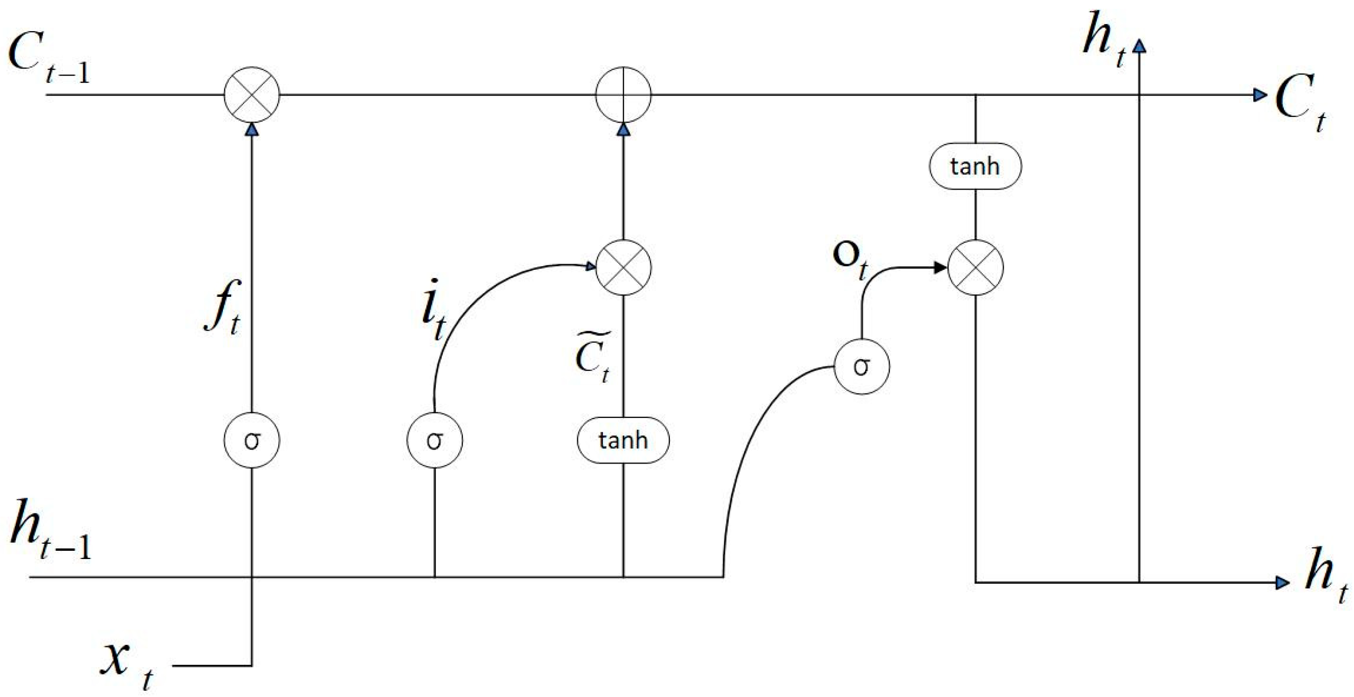
The LSTM predictive model, proposed by Hochreiter and Schmidhuber, has been used as an advanced version of RNN networks, overcoming the limitations of RNN networks by using hidden layer units called memory cells. The storage unit has a self-connection that stores the temporal state of the network and is controlled by three gates, called the input gate, output gate, and forget gate [
29,
30]. The basic structure of LSTM is shown in
Figure 1 below.
The calculation process of LSTM is as follows, and the forget gate determines which information should be forgotten from the cell state:
The input gate determines what information should be stored from the cell state, on the one hand to determine which information needs to be updated, and on the other hand to create a new updated state:
The output gate determines what information is ultimately output, and this output will be a filtered version based on the state of our cells:
Here,
represents the output of the previous hidden layer;
represents the current input;
is the Sigmoid function;
and
represent the weight matrix and bias matrix, respectively [
31].
3. Results
3.1. Spatial Distribution Characteristics of Regional Visibility in China
3.1.1. Spatial Distribution Characteristics of the Mean Value of Regional Visibility in China
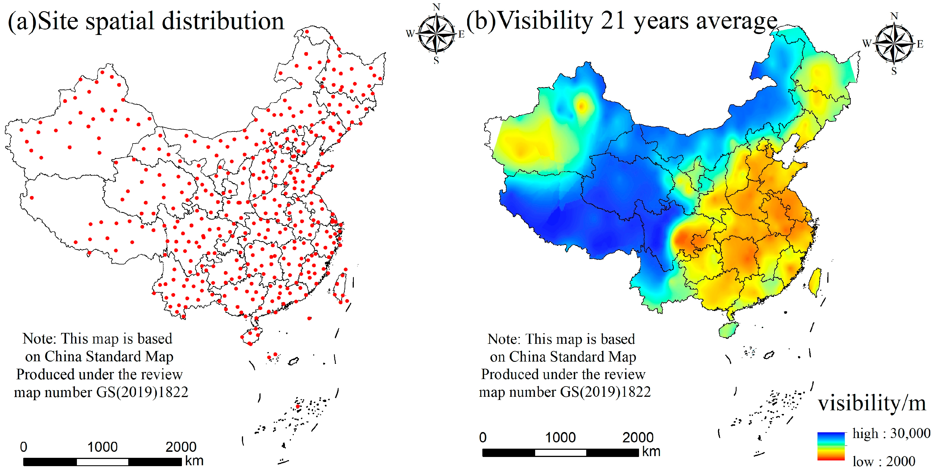
The continuous surface visibility data of 392 meteorological stations in the Chinese region were used, and the daily average visibility data of these 392 stations were converted into daily average extinction coefficient (EC) data, which is 3.912/visibility, according to the Koschmieder formula [
32], and the EC data were interpolated using the kriging interpolation method. Finally, the grid-based 21-year average EC data were calculated, and the grid-based 21-year average EC data were converted back to the grid-based 21-year average visibility data according to the Koschmieder formula, and the final results are shown in
Figure 2.
Figure 2a is a map of the spatial distribution of stations; observing
Figure 2b, we can see that the low visibility value areas are mainly distributed in East and Central China. The cities included in these two regions are some of the cities with faster economic development in China in the past 21 years, and their population is more densely distributed, while the rapid economic development brings a certain degree of air pollution, and the increase of PM2.5, car exhaust, and other kinds of particulate matter will contribute to the reduction in visibility. The medium-value areas are distributed in the Northeast and other regions, and the high-value areas are mainly distributed in Tibet, Qinghai, Gansu, and Inner Mongolia. These cities have open areas, and their economies are in a backward state compared with other medium-high visibility distribution areas, and the pollution is relatively light. Individual provinces and cities are in a state where both high and low visibility values exist.
3.1.2. Spatial Distribution Characteristics of the Average Visibility in Four Seasons
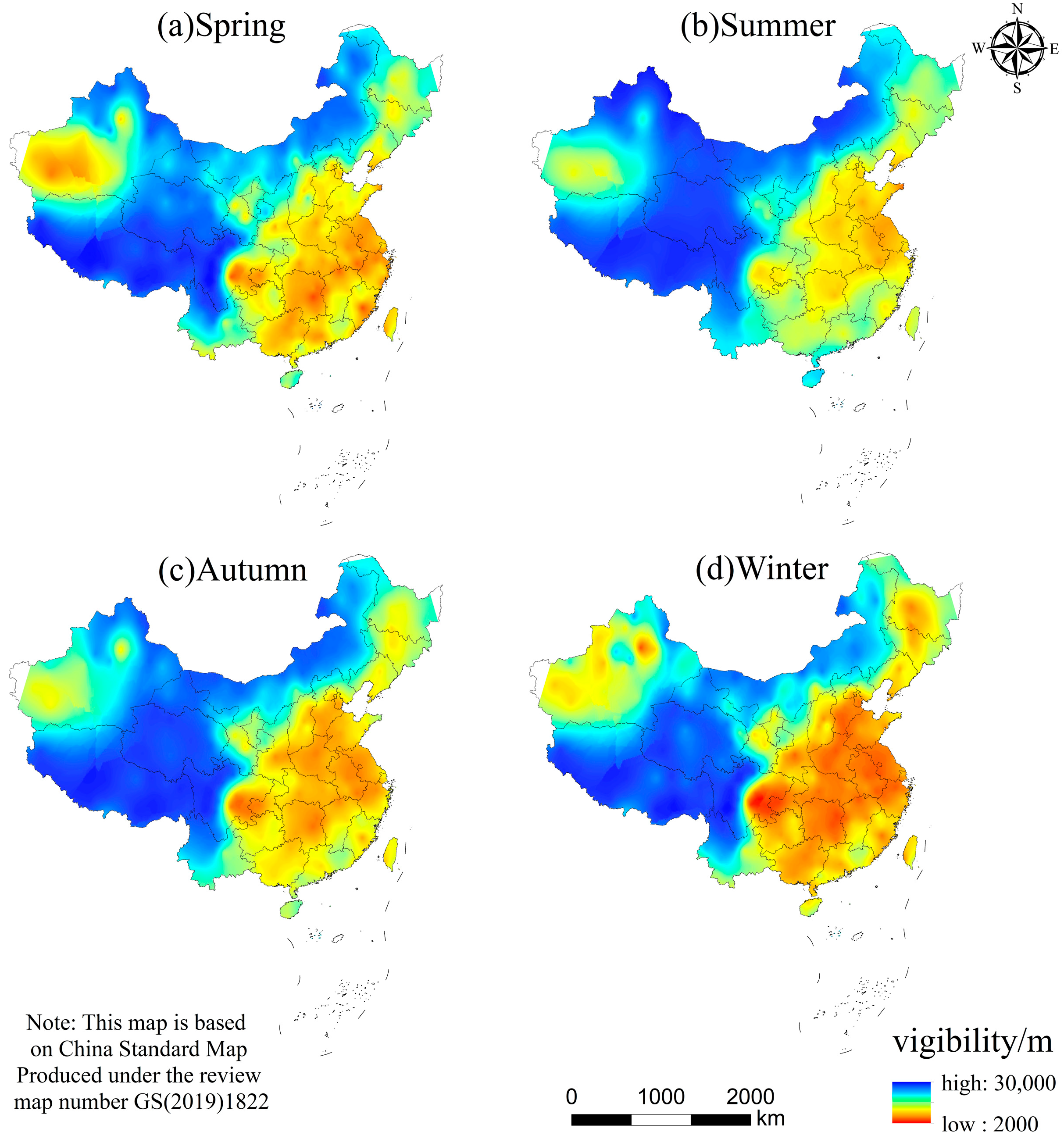
Similarly, the daily average visibility data of all stations were first transformed into EC daily average data, and the spatial distribution of visibility seasons was obtained according to the method in
Figure 2. Observing the distribution areas of high, medium, and low values of visibility, the spatial distribution of visibility in the four seasons in the four pictures in
Figure 3 is basically consistent with the spatial distribution of the average visibility in 21 years. Overall, the average visibility is highest in summer and lowest in winter.
3.2. Analysis of Time-Frequency Domain Variation of Regional Visibility in China
3.2.1. The Annual Average Change of Visibility in China and the Test of the MK Mutation Point
The visibility data recorded at meteorological stations in the region of China from 2001 to 2021 were averaged year by year as shown in
Figure 4a, and the visibility showed a decreasing trend from 2001 to 2015, with the highest value of about 19,012.1 m in 2001 and the lowest value of about 16,340.5 m in 2015, and the visibility was on an increasing trend after 2015. In the past 21 years, visibility has been declining generally, with a decreasing rate of about 59.56 m/a.
The MK mutation point test for the year-by-year averaged visibility data is plotted in
Figure 4b, where the intersection of the red line (UF curve) and the black line (UB curve) is between the two critical straight lines at
, satisfying the 95% confidence level. The values of UF curves were less than 0 from 2001 to 2021, indicating a decreasing trend in visibility from 2001 to 2021, which is consistent with the conclusion obtained from the interannual trend, and the decreasing abrupt change is known to be around 2003 by observation, where the UF value exceeds the critical value
after 2004, so the decreasing trend in visibility in the Chinese region is significant after 2004.
3.2.2. Seasonal Variation Trend in Regional Visibility in China
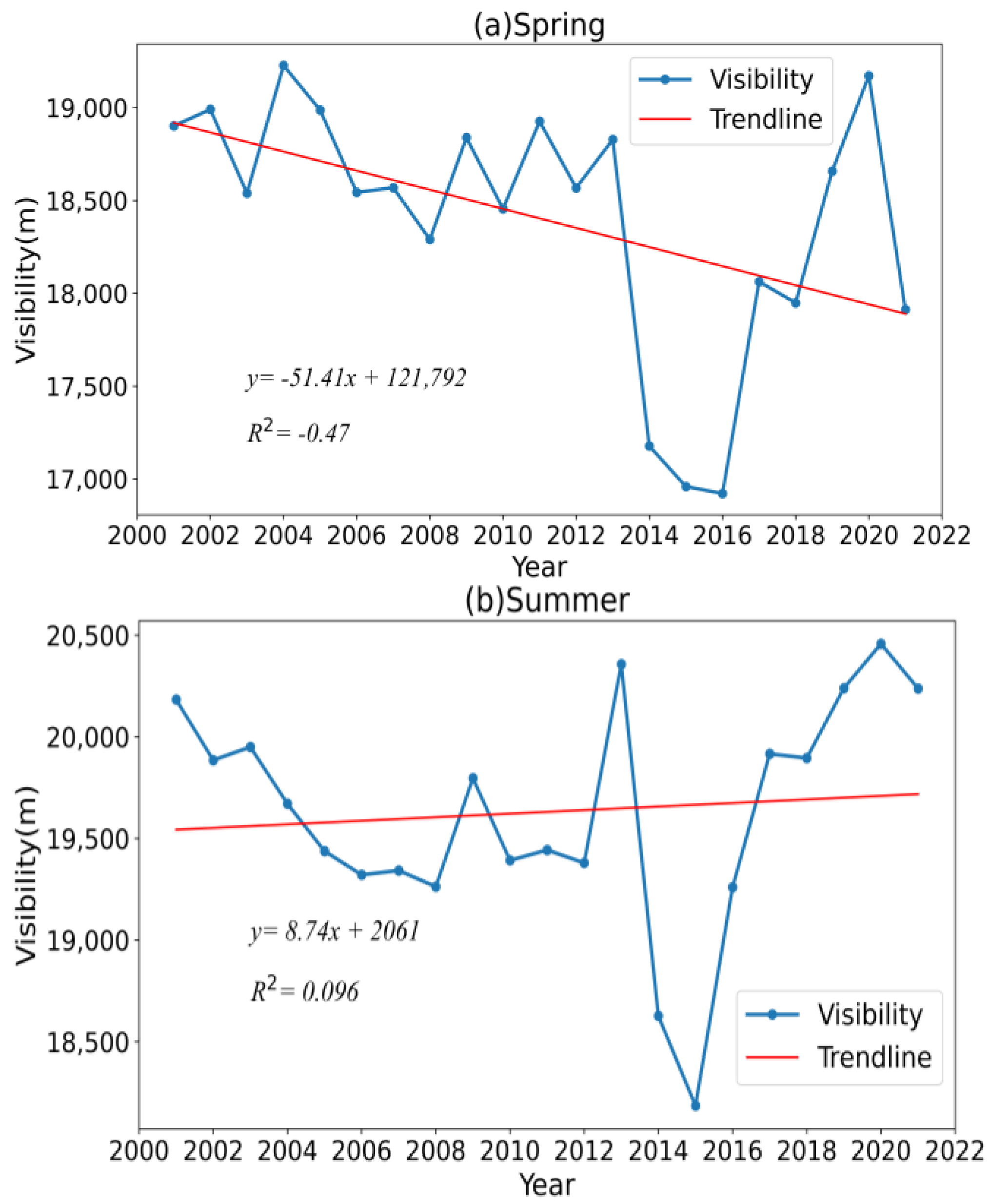
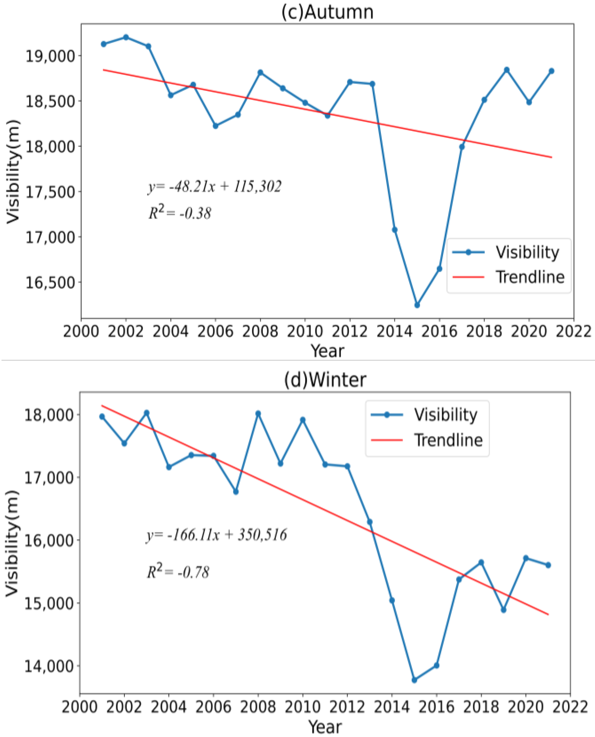
Figure 5 shows the seasonal trends in regional visibility in China. The trends in visibility in the four seasons and its annual average from 2001 to 2021 all show roughly a V-shaped trend. It can be seen that except for summer, the overall visibility trend was decreasing in spring, autumn, and winter. The decreasing rate of visibility in spring was about 51.41 m/a, the peak value of visibility was about 19,226.8 m in 2004, and the valley value was about 16,921.5 m in 2016. The rising rate of visibility in summer was about 8.74 m/a, the peak value of visibility was about 20,457.6 m in 2020, and the valley value was about 18,185.2 m in 2015. The declining rate of visibility in autumn was about 48.21 m/a, the peak value of visibility was about 19,202.8 m in 2002, and the valley value was about 16,246.6 m in 2015. The decreasing rate of visibility in winter was about 166.11 m/a, the peak value of visibility was about 18,026.2 m in 2003, and the valley value was about 13,772.8 m in 2015. The rate of decline in winter was the largest, so it has the greatest impact on the downward trend in visibility and plays a major role, followed by spring and autumn, with the least impact in summer. The average visibility in spring, summer, autumn, and winter was 18,403.2 m, 19,630.5 m, 18,359.9 m, and 16,477.7 m, respectively, with the maximum average visibility in summer and the minimum in winter, which is consistent with the conclusions obtained from the distribution of the average visibility spatial characteristics in four seasons studied earlier.
In
Figure 4 and
Figure 5, it can be observed that the regional visibility in China changed significantly less between 2013 and 2015 and then changed back to an increasing trend after 2016. To investigate the reasons for this, the literature on regional environmental pollution in China during this period was reviewed. Feng et al. [
33] pointed out that in early 2013, the haze was widespread and long-lasting, affecting 17 provinces (autonomous regions and municipalities directly under the central government), accounting for about a quarter of China’s land area and affecting 600 million people. Severe haze pollution since 2013 has required the Chinese government to strengthen its efforts to combat PM2.5, nitrogen oxides, and dust haze, and this frequent haze was an important factor contributing to the 2014 revision of “the Environmental Protection Law”. Zhang et al. [
34] found that meteorological conditions deteriorated and aerosol pollution was severe in key areas of China in 2014 and 2015 relative to 2013, and was mitigated in 2016 and 2017. Liu et al. [
35] pointed out that the annual average mass concentrations of PM2.5 monitored in 74 major cities in China in 2013 and 2015 were 2.1 and 1.4 times higher than the maximum permissible mass concentration values required by China’s national ambient air quality standards for Class 2, respectively, and more than 5 times higher than the maximum permissible mass concentration values recommended by the World Health Organization air quality guidelines [
36]. All of the above studies could indicate that there was severe air pollution in China from 2013 to 2015, which could be the direct cause of the significant change in visibility in 2014 and the trough in atmospheric visibility in 2015. China introduced “the Air Pollution Prevention and Control Plan” in 2013 and has taken a series of various measures to improve environmental pollution. Using a three-year (2015–2017) dataset containing pollutants, such as PM2.5, Silver et al. [
37] found significant decreases in PM 2.5 and SO2 concentrations at 53% and 59% of sites. The increase in regional visibility in China after 2015 is the result of the joint efforts of the Chinese government to introduce and revise relevant policies, and the people to reduce emissions and strictly comply with relevant policies.
3.2.3. Inspection of MK Mutation Point of Visibility in Four Seasons in China
The MK mutation point test (shown in
Figure 6) was performed on the four-season visibility data for the Chinese region from 2001 to 2021, and it can be seen that the UF and UB curves have only one intersection point for all four seasons during these 21 years, and the intersection points are all within the critical value
, which has some reference significance. Observing the winter UF curves, the values of UF are less than 0 from 2004 to 2021, and the intersection of UF and UB is in 2011, which indicates a general decreasing trend n visibility in winter from 2004 to 2021, and the decreasing abrupt change in visibility occurs around 2011. Among them, the UF curve of winter visibility exceeded the critical value after 2013, indicating a significant decreasing trend in winter visibility after 2013. Similarly, observing the UF and UB curves in summer, we can obtain the sudden change point in summer around 2019. The UF curves for both spring and fall were less than 0 after 2006, indicating that both spring and fall visibility showed an overall decreasing trend after 2006, and the UF values for spring and fall exceeded the critical values around 2014, which indicates a significant decreasing trend in spring and fall visibility after 2014.
3.2.4. Regional Visibility Discrete Wavelet Transform in China
Calculate the monthly mean value of visibility for 252 consecutive months in China from 2001 to 2021, and take it as the research object of the visibility frequency domain change. This paper will use the discrete wavelet transform to decompose noise reduction and reconstruct the visibility time series of 252 months and then perform continuous wavelet transform on the reconstructed visibility time series, which will make the obtained period more accurate.
Considering the visibility time series and the existing wavelet basis functions in Matlab applicable to DWT, sym5 wavelet basis is used to decompose and reconstruct the visibility time series at level 1. The original visibility time series is first decomposed at level 1 to complete the conversion of the signal from the time domain to the wavelet domain.
Figure 7a shows the low-frequency approximate components of the visibility time series after level 1 decomposition, and
Figure 7b shows the high-frequency detailed components. It can be seen that the noise of the original visibility time series is mainly concentrated in the high frequency detail component, so noise reduction is needed for the high frequency component.
Use the wden () function to perform threshold denoising based on the high-frequency detail component, and then, use the low-frequency approximate component and the high-frequency detail component after denoising to reconstruct and obtain the reconstructed visibility time series. The wden () function serves to perform automatic one-dimensional denoising using the wavelet transform, which is used in one of the following forms: XD = wden (X, TPTR, SORH, SCAL, N, WNAME). Here, XD indicates the denoised signal; X indicates the noisy signal to be processed; TPTR indicates the threshold selection rule specified as a string; SOPH indicates whether to specify soft or hard threshold denoising; SCAL defines the type of threshold rescaling; N indicates the level of the wavelet transform; and WNAME indicates which wavelet you are using for denoising, that is, the wavelet basis.
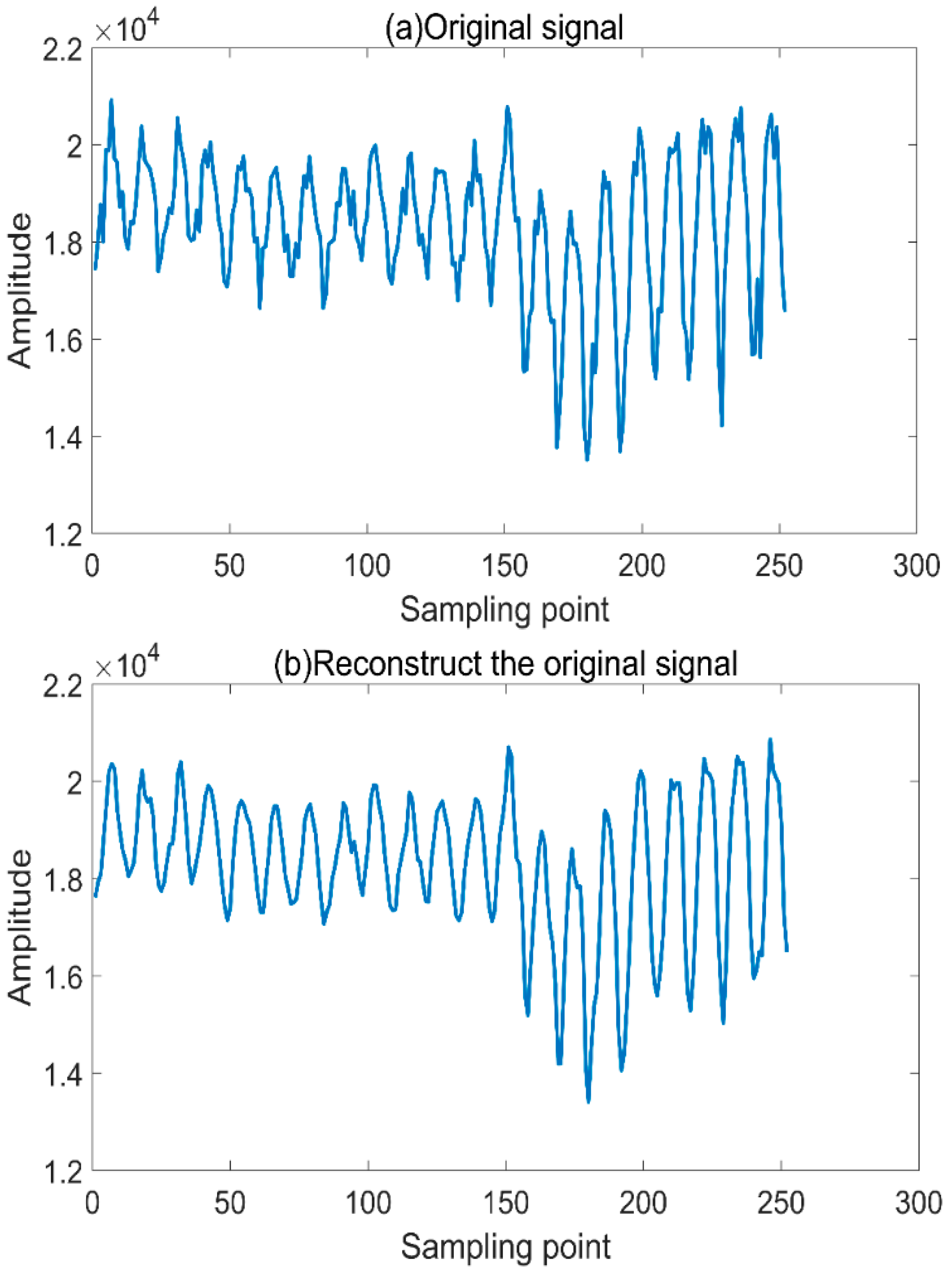
Figure 8a below is the original visibility time series, and
Figure 8b is the reconstructed visibility time series. Compared with the original series, the trend of the two is consistent and the error is small, with high data fidelity.
3.2.5. Continuous Wavelet Transform for Regional Visibility in China
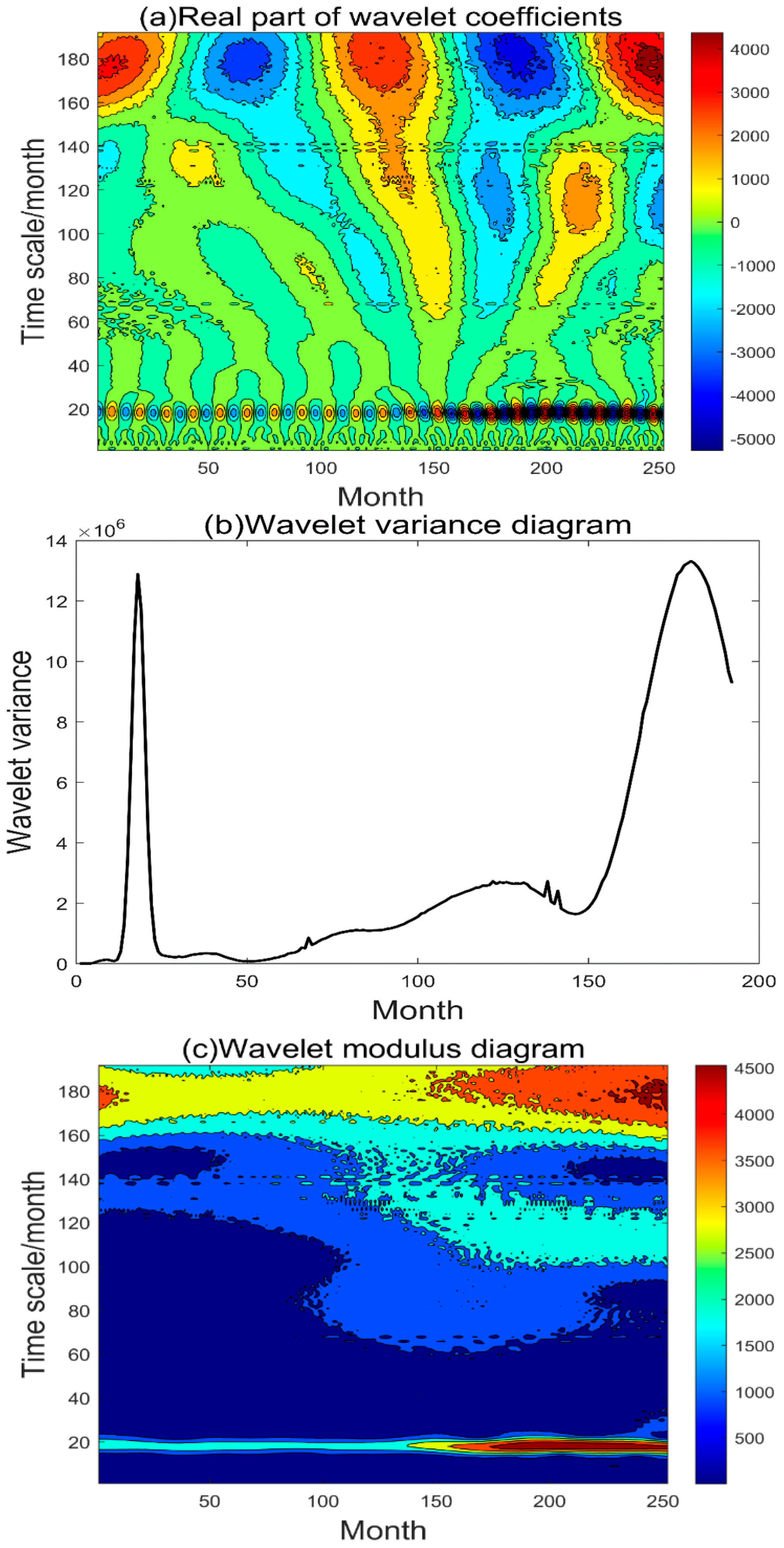
The reconstructed visibility time series of 252 months from 2001 to 2021 are subjected to Morlet continuous wavelet transform to study the variation pattern of visibility in the frequency domain in the Chinese region, and it can be seen that the visibility variation in the Chinese region contains multiple nested cycles.
Figure 9a shows the wavelet real part isolinear plot, and the observation shows that on the time scale the Chinese regional visibility has a period of 9 months, 18–20 months, 120 months, and 180 months. From
Figure 9b, we can see that there are two most obvious peaks in the wavelet variogram, and these two obvious peaks correspond to a time scale of 18 and 180 months, respectively. Moreover, the peak corresponding to 180 months is the largest, indicating that the 180-month cycle of regional visibility change in China has the most intense oscillation and is the first main cycle of regional visibility change in China, and the peak corresponding to 18 months is the second, which is the second main cycle of regional visibility change in China.
Figure 9c shows the time-scale distribution corresponding to the modal values of wavelet coefficients of regional visibility in China, where the larger the modal values of wavelet coefficients, the stronger the corresponding scale periodicity. It can be seen that the modal value of the regional visibility variation in China is the largest around the 180-month time scale, indicating the strongest cyclic variation, followed by the cyclic variation around the 18-month time scale, and the rest is not significant.
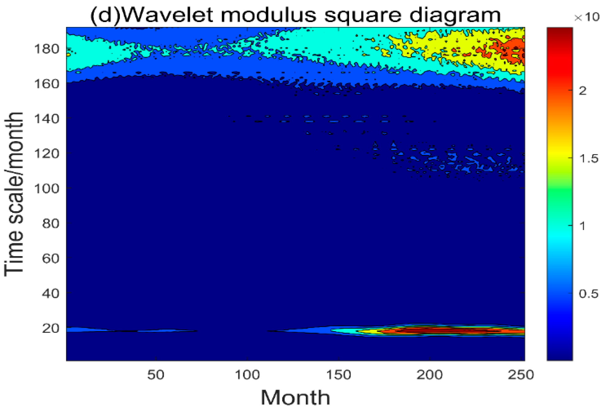
Figure 9d shows the time-scale distribution corresponding to the mode squares of wavelet coefficients for regional visibility in China. The mode squares of wavelet coefficients are equivalent to wavelet energy spectra, and the stronger the energy, the more significant the period. It can be seen that regional visibility in China oscillates with strong energy around 180- and 18-month time scales, and the cycle is the most significant.
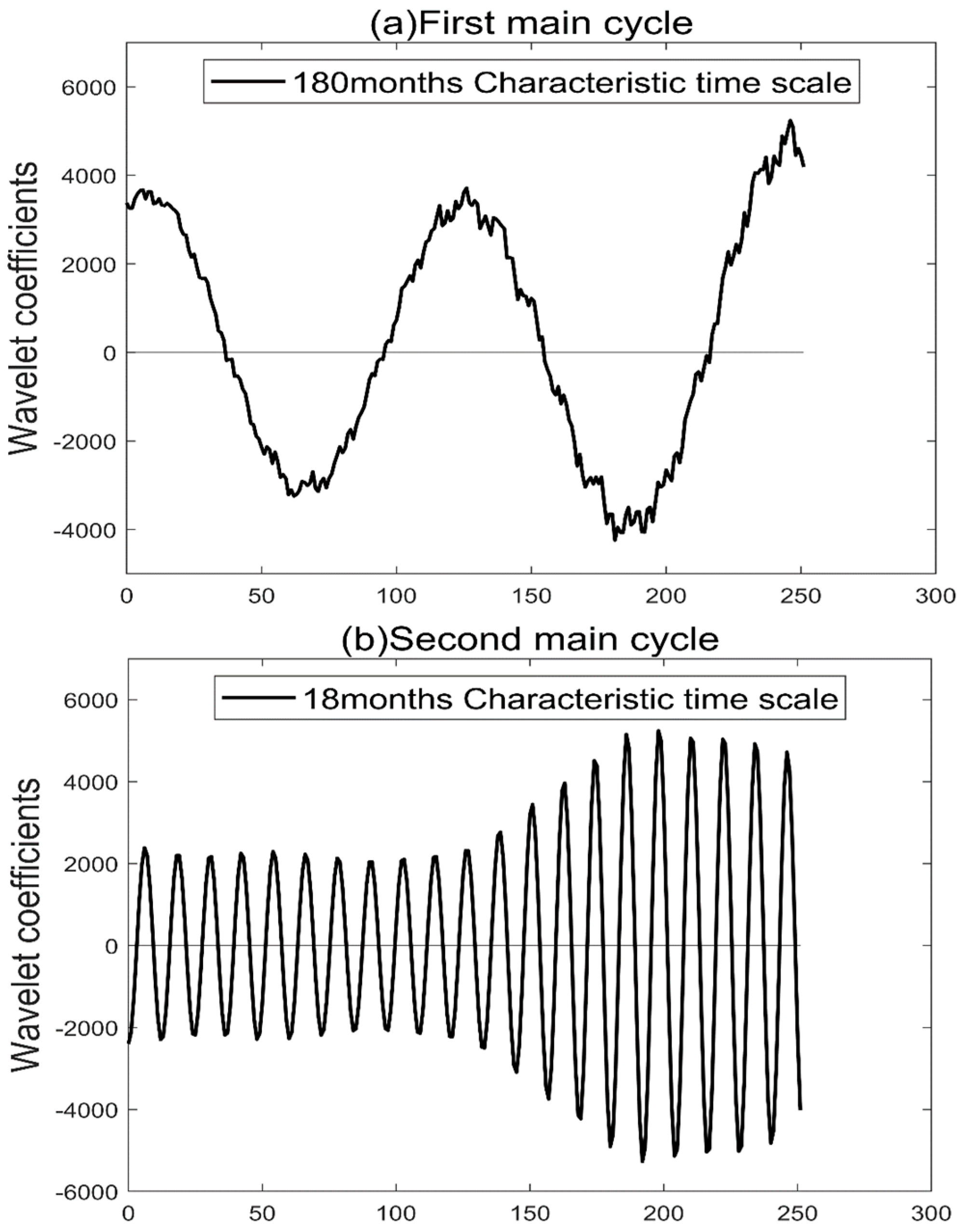
In order to further study the influence of multi-scale features on the visibility changes in China, the wavelet coefficient maps corresponding to the first main period and the second main period (the changing trend of the main period) are drawn as follows. From
Figure 10a, it can be seen that under the characteristic time scale of 180 months in the first main cycle, the average period of regional visibility variation in China is about 123 months, and it experiences two periods of high–low variation in 252 consecutive months from 2001 to 2021. From
Figure 10b, the average period of regional visibility variation in China is about 12 months under the characteristic 18-month time scale of the second main cycle, and it experiences 21 periods of high–low variation in 252 consecutive months from 2001 to 2021.
3.3. The Relationship between the Economy and Visibility Changes in Different Provinces and Cities in the Chinese Region
The average values of regional gross domestic product from 2002 to 2021 were obtained for each of the 31 provinces and cities in the Chinese region, the average values of visibility from 2002 to 2021 were also obtained for each of these 31 provinces and cities, and the relationship between the economy and the corresponding visibility of different provinces and cities was plotted.
Table 1 shows the serial numbers corresponding to the different provinces and cities in the Chinese region. As shown in
Figure 11, the Pearson correlation coefficient between the economy and visibility of different provinces and cities is −0.494, and there is a strong negative correlation between the two, and the visibility of provinces and cities with a higher economy is generally lower; for example, the average value of the GDP of Jiangsu Province in the past 20 years is 541.29 billion yuan, but the average value of visibility is only 10,049.4 m. The visibility corresponding to the provinces and cities with lower economy is generally higher; for example, the average value of the GDP in Tibet in the past 20 years is 83.398 billion yuan, and the average value of visibility is as high as 28,330.5 m.
However, there is not a simple negative correlation between the economy and visibility. Ma et al. [
38] studied, in detail, the relationship between regional PM2.5 concentrations and the economy in China. High-GDP areas with high pollution, such as cities in Jiangsu, Zhejiang, and Shandong, which are affected by urbanization, energy use and population density, and motor vehicle ownership, have higher PM2.5 concentrations. Equally polluted are areas with a low GDP, such as cities in Anhui, Hunan, Hubei, and Guangxi, where low energy utilization and more pollution-intensive industries are the main causes of higher PM2.5 concentrations in these cities. The non-polluted areas with low PM2.5 concentrations, such as Tibet, Gansu, and Qinghai, are generally not economically developed, with a very low GDP, and these areas are at higher altitudes where particulate matter, such as PM2.5, does not easily gather. The areas of high and low PM2.5 concentration distributions studied by Ma et al. correspond to each other with the areas of low and high visibility distribution in this paper, and it further follows that regions with high PM2.5 concentrations have low visibility, but not necessarily a high GDP, and there are many cities in China that are still developing, while regions with low PM2.5 concentrations have high visibility and a generally low GDP.
3.4. Construction and Analysis of Regional Visibility Prediction Model in China
3.4.1. SARIMA Forecasting Model
Using the monthly average of 252 months of visibility in China from 2001 to 2021 as the original forecast data,
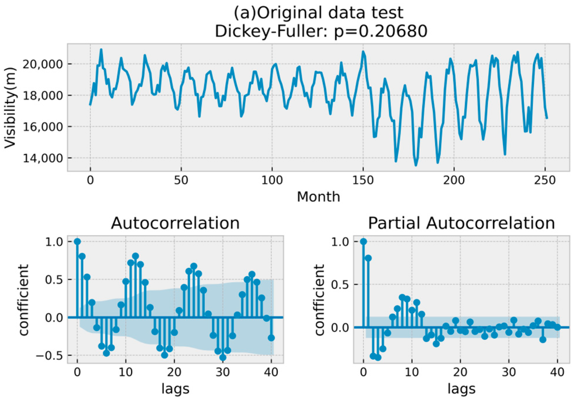
Figure 12a shows the time series of the original data and its autocorrelation and partial correlation diagrams. The lag coefficient in the autocorrelation diagram is set to 40. Observing the visibility raw time series, we can see that it has obvious seasonality, the visibility varies in the range of 13,500 m to 21,000 m, and there are some decreasing and increasing trends. The Dickey–Fuller unit root test was performed on the original series and yielded a
p-value = 0.2068 > 0.05, which means that the null hypothesis was accepted and the original visibility time series was determined to be non-stationary. The first thing needed to construct the SARIMA model is a smooth series, so the seasonality of the visibility time series should be eliminated and the seasonal difference should be processed, and since the year is 12 months, the seasonal length is set to 12 to obtain the seasonal difference test (
Figure 12b). It was observed that the
p-value = 0.01107 < 0.05; among the Dickey–Fuller unit root test, the periodicity of the shaded part in the autocorrelation plot disappeared, and the seasonality of the original visibility time series was eliminated and changed to a smooth series. Due to the presence of the trend term in the series, there were still more significant time lags in the autocorrelation and bias correlation plots, so it was necessary to continue the first-order differencing process.
Figure 12c shows the test plot obtained by first-order difference processing. From
Figure 12b,c, the visibility time series changes from irregular oscillation above and below 0 to stable oscillation above and below 0. The
p-value is =0.00000 in the Dickey–Fuller unit root test, and the
p-value is less than 0.01 based on white noise test. The visibility time series at this point can then be used for prediction model construction.
After the previous processing, it is necessary to determine the parameters of the SARIMA forecasting model; p represents the maximum lag value, which can be observed in PACF. Through
Figure 12c, it is initially assumed that
p = 2. Similarly, q can be found in ACF, assuming q = 2. Since first-order differencing was performed, d = 1; s is the seasonal period, so s = 12; and since seasonal differencing was performed, D = 1. Finally, the parameters were adjusted according to the AIC criterion, and the final optimal parametric prediction model for the monthly average time series of regional visibility in China was SARIMA (2,1,2) (0,1,1,12).
The residual test of the determined SARIMA prediction model is shown in
Figure 12d, and it is observed that the lagged values of the autocorrelation and partial correlation plots are almost within the shaded part, while the
p-value = 0.00000, which indicates that the parametric model works well and can predict the future values of the visibility time series.
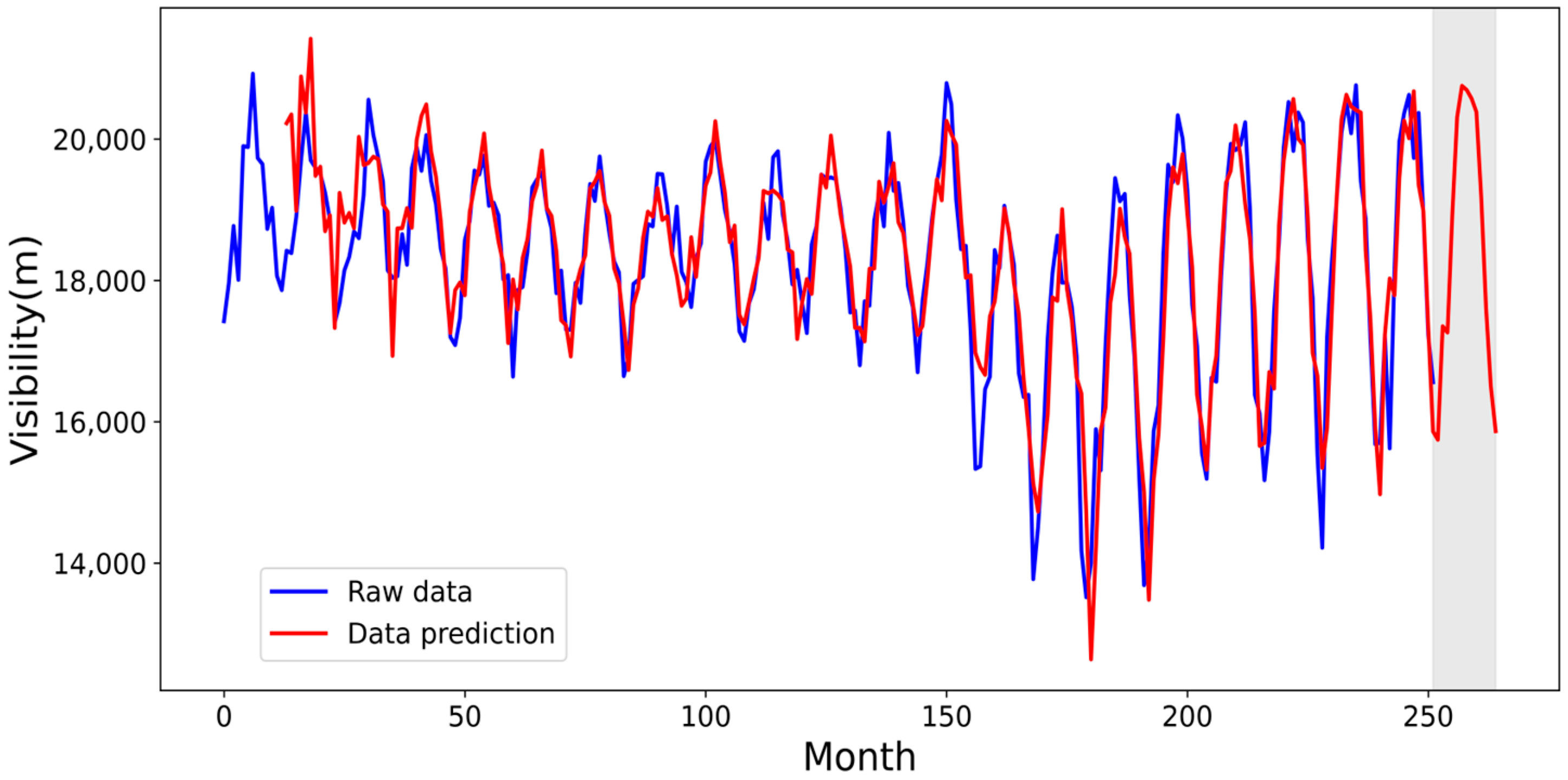
The predicted time series of visibility in China for the next 12 months are plotted as shown in
Figure 13, where the horizontal coordinates represent months and the vertical coordinates are visibility. The blue line in the figure represents the original visibility time series, the red line represents the visibility prediction time series, and it can be observed that there is a high degree of overlap between the two. The evaluation index of the prediction model was calculated, and the root mean square error (RMSE) was 655.56, the mean absolute percentage error (MAPE) was 0.028%, and the goodness of fit (
) was 0.807. The SARIMA prediction model constructed in this study has a high prediction accuracy and good results. The shaded part has a slight fluctuating upward trend of visibility for the next 12 months in the Chinese region, which has some reference value.
3.4.2. LSTM Prediction Model
In the following, we will continue to construct a long- and short-term memory neural network to predict the visibility in the Chinese region, and the monthly averages of visibility for 252 months from 2001 to 2021 will be used as the original data. The first two modules in python, Pandas, and NumPy are used to convert the data to floating point values, which are more suitable for modeling with neural networks. Since LSTM is sensitive to the size of the input data, especially when using the sigmoid (default) or tanh activation functions, the data need to be scaled to the range of 0 to 1, that is, normalized. LSTM expects the input data (X) to provide an array structure in the form of (samples, time steps, features), divides the data 7:3 into training and test sets, and uses numpy.reshape () to transform the divided dataset into this structure after input.
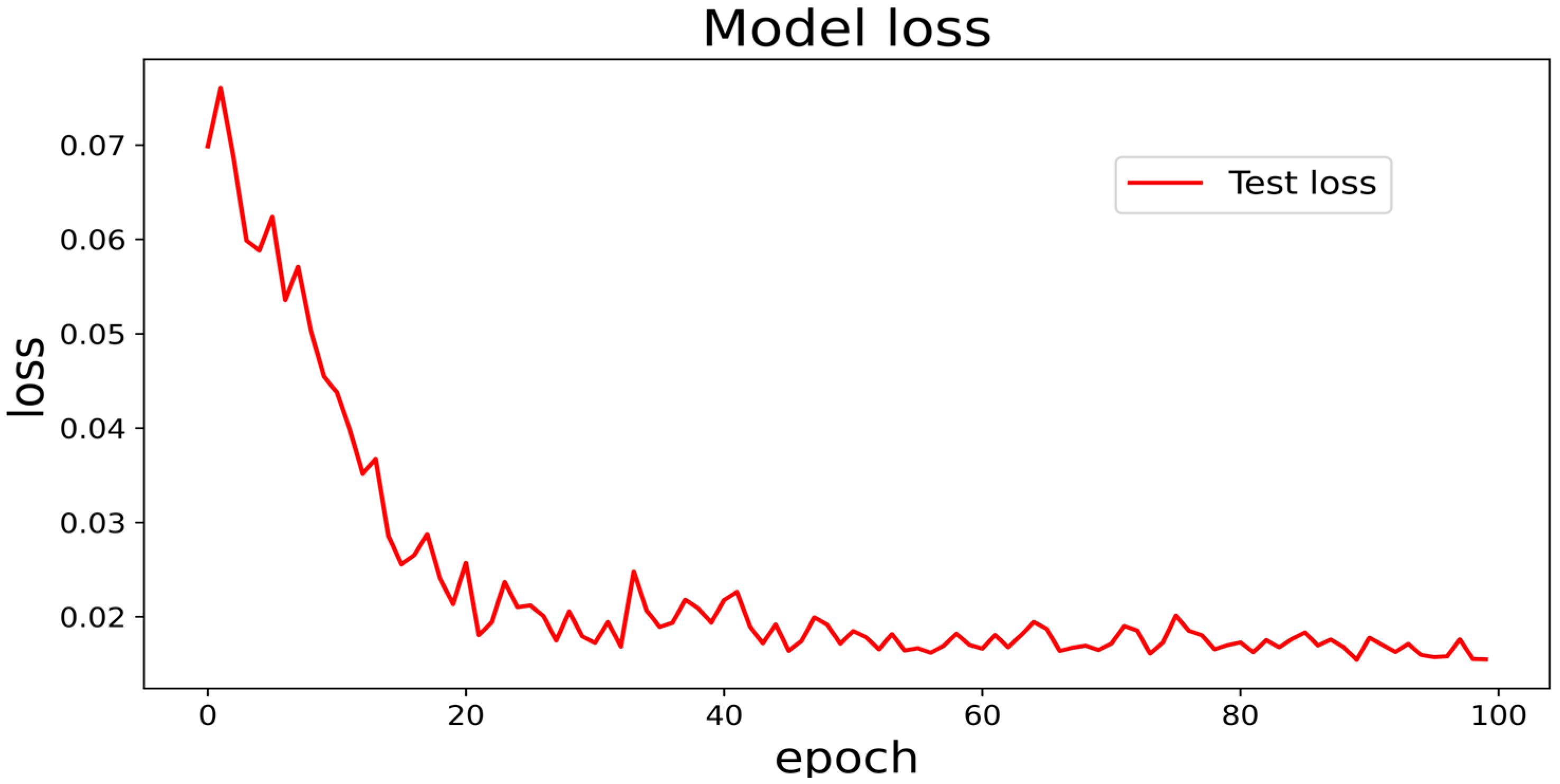
The LSTM network designed here has 1 input layer, the hidden dimension is 100, 1 output layer, using the tanh activation function, 100 epochs of network training, and a batch number set to 1, and the network structure is shown in the following
Table 2.
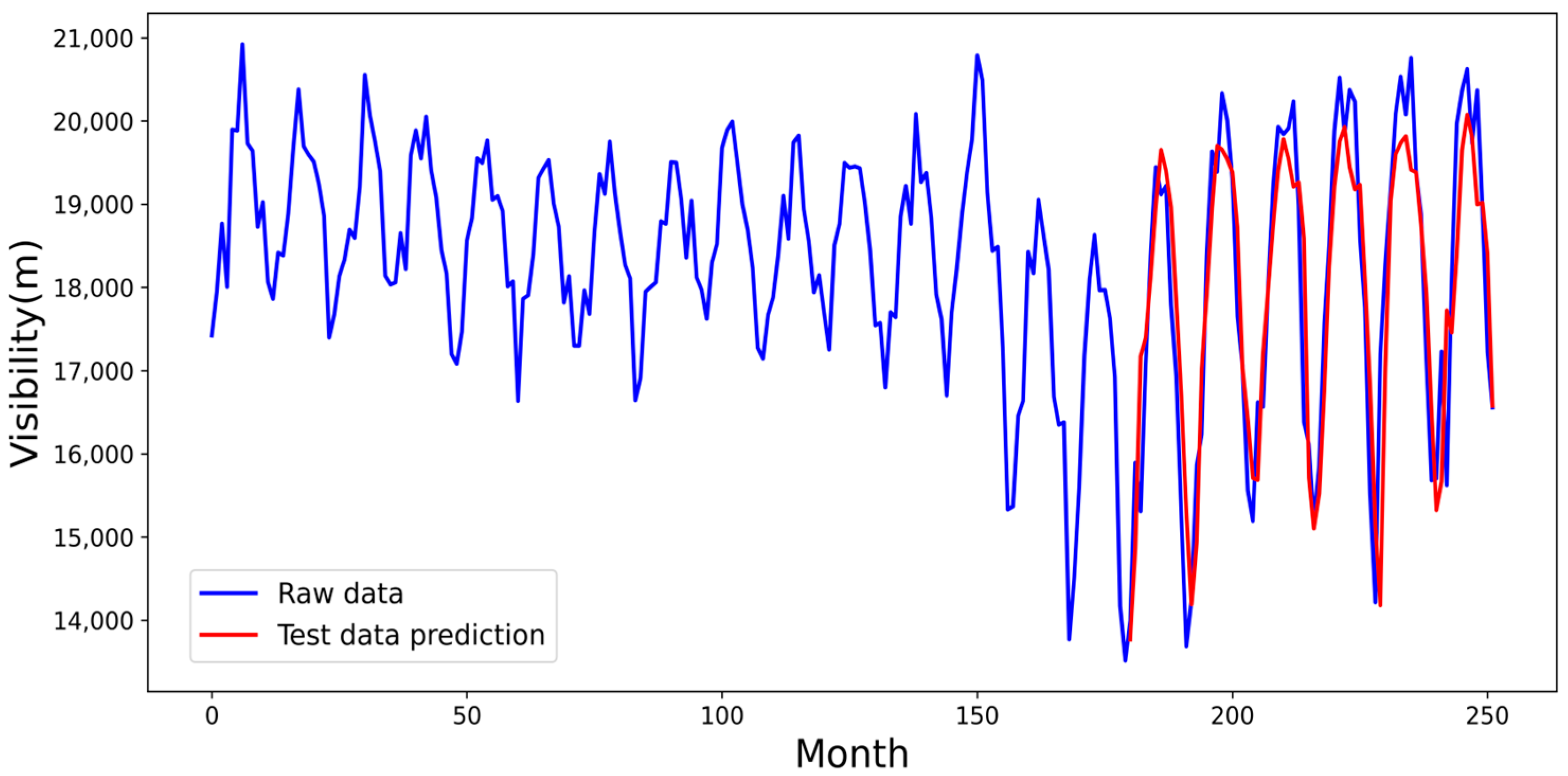
Through model training, the prediction series of regional visibility in China is obtained, as shown in
Figure 14 below. The red line is the prediction result for a total of 72 months, the relevant assessment index is obtained, the RMSE is 921.71, MAPE is 0.041%, and the
is 0.776, which is a good prediction effect of the model. As shown in
Figure 15, observing the loss function curve, the loss error is stable at 0.02 up and down around 40 times for training, the model accuracy is high, and the error is small compared with the real value.
4. Discussion
Most scholars have analyzed visibility indirectly, mainly by studying aerosols and other meteorological factors. In 1967, Horvath [
39] studied the relationship between the extinction coefficient and visibility and showed that in most cases, the average extinction coefficient between the target and the observer determines the visibility. Wang et al. [
40] investigated the factors influencing visibility in Beijing using relevant data measured at 12 stations in the city and showed that visibility is influenced by meteorological conditions, in addition to particulate matter concentrations. Li et al. [
41] used a source-oriented community multiscale air quality model to quantify the source contribution to visibility impairment in China in 2013, and found that industrial and residential emissions were the most important sources of visibility impairment in winter. It can be found that scholars mainly focus on visibility-influencing factors, but the highlight of this paper is that the parameter of the study is the Chinese regional visibility data itself, which directly analyzes various long-term changes (including the time domain and frequency domain) of Chinese regional visibility in detail and draws relevant conclusions.
In this paper, we found that the average visibility in summer was the highest and the average visibility in winter was the lowest, which is similar to the findings of Chang et al. [
42] in their study of visibility trends in six megacities in the Chinese region from 1973 to 2007. Chang et al. found that five of the six cities had the worst visibility in winter and four had better visibility in summer than in other seasons. The possible reasons given in Chang et al.’s paper are that visibility is worse in winter due to low temperatures and increased coal burning for heating and better in summer when high temperatures induce wind speeds and strong diffusion. In addition, Li et al. [
43] studied, in detail, the temporal evolution of interannual and seasonal trends in extinction coefficients from 1980 to 2004 in six regions of the Chinese region and found that winter and autumn showed the largest trends in all regions and indicated that anthropogenic aerosols were the dominant pollutant species in these two seasons. China has experienced rapid economic development in the last 20 years, but rural areas of China still make up a large part of the country, and the increase in coal burning in winter and the rise in the concentration of aerosol particles, such as anthropogenic PM2.5, are possible causes of the lowest visibility in winter. In studying long-term atmospheric visibility, sunshine duration, and precipitation trends in South China, Liao et al. [
44] found that visibility and rainfall may be related, with visibility becoming higher with more short-term rainfall and the opposite in the long term. Here, we speculate that the reason for high visibility in summer may also be related to frequent short-term rainfall in summer.
This paper also explores the intrinsic link among visibility, PM2.5, and the economy through relevant literature. Economically developed areas are densely populated and have a high concentration of particulate matter emissions, which leads to higher PM2.5 concentrations and consequently lower visibility. Areas with lower economies and higher altitudes, such as cities in Gansu, Qinghai, Tibet, and Xinjiang, have relatively low atmospheric stability, which is not conducive to the accumulation of particulate pollutants, such as PM2.5, resulting in high visibility, and the concentration of particulate pollutants, such as PM2.5, is the link among these three.
5. Conclusions
Based on GSOD visibility site data and GDP data, linear regression, an MK mutation point test, wavelet transform, and SARIMA model prediction are applied in this paper. The time-frequency domain and spatial distribution characteristics of regional visibility in China from January 2001 to December 2021 were studied in detail, revealing the influencing factors of visibility and making predictions of visibility, which are of great significance for further understanding visibility and the prevention and control of low visibility. This study led to the following conclusions.
Regional visibility in China has generally been on a downward trend for the past 21 years, and between 2013 and 2015 there was severe air pollution in the Chinese region, but in 2013, China adopted many air pollution-prevention strategies that effectively improved the pollution problem in just 3 to 5 years, which led to a significant upward trend in visibility after 2015. In the spatial distribution of the 21-year average of regional visibility in China, visibility has obvious regional distribution characteristics, with the East China region and Central China region being the regions with high values of visibility and Tibet and Qinghai and other places being the regions with low values of visibility. There is a certain connection between the economy and visibility of a region. Individual cities with a very low GDP are influenced by the population distribution, geographical altitude, and national policies, and their economic development is slow, so that particulate matter, such as PM2.5, is not easily gathered and the concentration of particulate pollutants is very low, resulting in very high visibility. In addition to some high-GDP cities with highly developed economies where visibility is very low, some areas with not very high GDP still have low visibility, such as Anhui, Hunan, and Hubei, where the population distribution is concentrated and the emission of various particulate matter is concentrated, also making the concentration of PM2.5 and other particulate matter high and thus contributing to low visibility. The spatial distribution of regional visibility in China in all seasons is basically consistent with the spatial distribution of the 21-year average, and the seasons show lower visibility in winter and higher visibility in summer. The trends of the four seasons in visibility in China are basically consistent with the interannual variations, except for a slight upward trend in summer, all of them are decreasing, and there is only one abrupt change point in both the four seasons and the interannual variations.
Using DWT to reconstruct the 252-month monthly average time series of regional visibility in China based on noise reduction and then using CWT on the reconstructed visibility series, it is concluded that there are time scales of 9-month, 18–20-month, 120-month, and 180-month cycles of regional visibility in China, and the first main cycle is 180 months and the second main cycle is 18 months. Under the characteristic time scale of 180 months in the first main cycle, the average period of regional visibility variation in China is about 123 months, and under the characteristic time scale of 18 months in the second main cycle, the average period of regional visibility variation in China is about 12 months. SARIMA and LSTM were used to predict the monthly average visibility data in China, and both of them achieved better evaluation indexes. The prediction effect of SARIMA was slightly better than LSTM, and the future changes in visibility in China may show an upward trend.
Finally, although this paper gives a reasonable explanation for the apparent change in the visibility trend after 2013, further verification is still needed regarding the change in specific values of visibility after 2013, and subsequent studies need to pay attention to this issue. Moreover, the change in visibility is influenced by many factors, and if we want to continue to dig deeper into the mechanism of its change, more and more complete data may be needed for further research.
