
Total Electron Content PCA-NN Prediction Model for South-European Middle Latitudes


Abstract
1. Introduction
2. Data
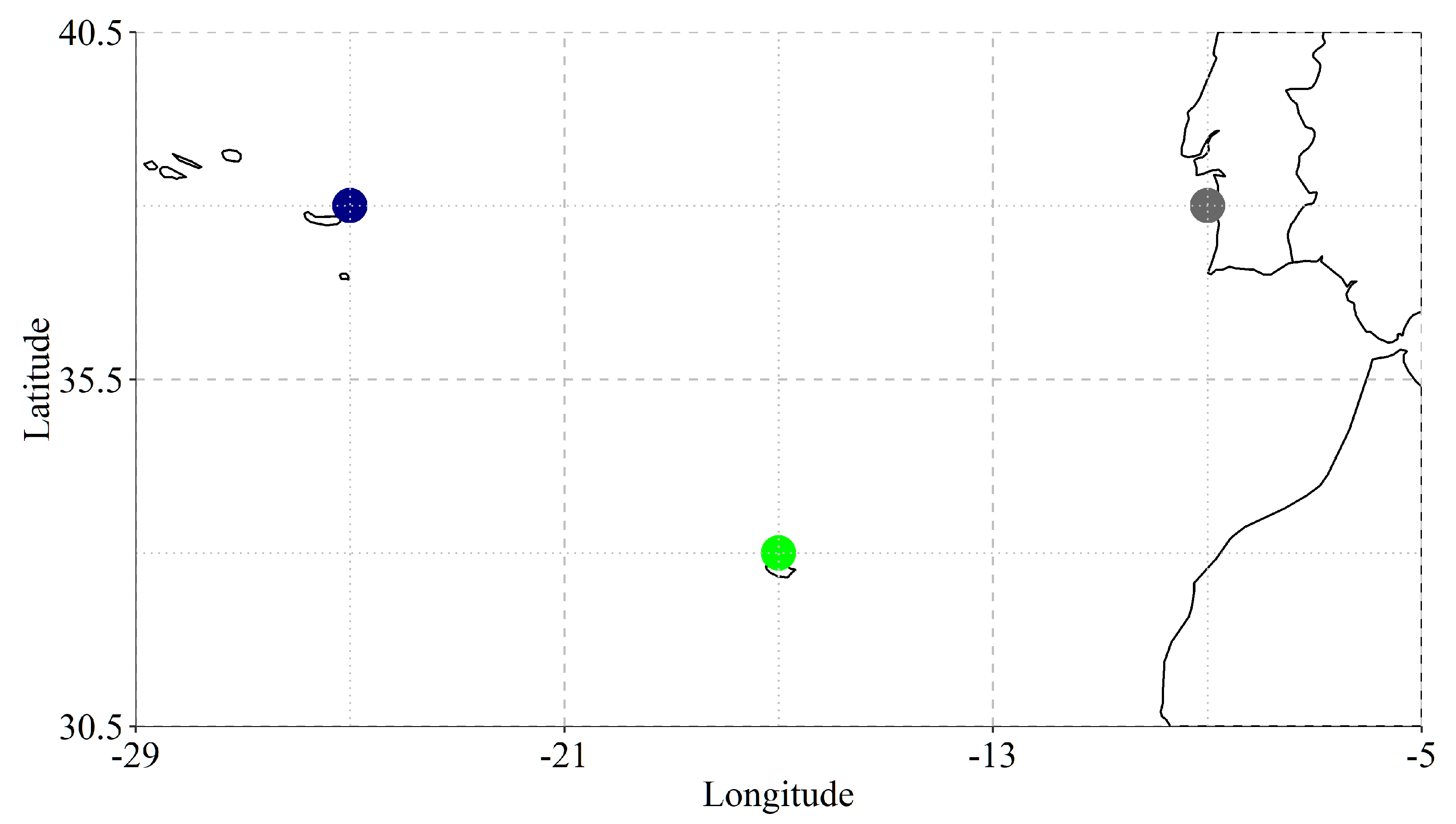
2.1. TEC Data
2.2. Space Weather Parameters
- Parameters characterizing the interplanetary medium:
- 1.1.
- scalar of the interplanetary magnetic field (IMF), B in nT;
- 1.2.
- the X, Y and Z components of IMF in the GSM frame, BX, BY and BZ, respectively, all in nT;
- 1.3.
- the solar wind flow pressure (p in nPa), proton density (n in n/cm3), and plasma speed (v in km/s).
- Geomagnetic indices:
- 2.1.
- the disturbance-time index Dst;
- 2.2.
- the global ap index;
- 2.3.
- the daily sums of the Kp index;
- 2.4.
- the auroral electrojet index AE characterizing the auroral activity in the polar regions.
- Parameters characterizing the solar UV and XR fluxes:
- 3.1.
- proxies for the solar UV irradiance:
- 3.2.
- a proxy for the solar XR irradiance: the measurements of the Solar EUV Experiment (SEE) for the NASA TIMED mission at the wavelength 0.5 nm, hereafter XR;
- 3.3.
- the daily number of the solar flares
- 3.3.1.
- of the B and C classes, hereafter Number of C flares, C or C.f.;
- 3.3.2.
- of the class M, hereafter Number of M flares, M or M.f.;
- 3.3.3.
- total daily number of the solar flares of any class from B to X, hereafter Number of flares, N, or N.f.;
3. PCA-NN Model Prototype Development
3.1. PCA-Based Models
3.2. Forecasting Skills (Metrics)
3.3. PCA-MRM Model
3.4. PCA-NN Model
3.4.1. NN Algorithm
- Input datasets of different lengths L;
- NNs built with the input SWp series with lag equals only to 1 or 2 days, and NNs built with the input SWp series with lags of 1 and 2 days together;
- NNs of different depths: from 5 to 1 hidden layers;
- NNs with different number of nodes per a hidden layer.
- In general, the input dataset with L = 31 days (same as for the PCA-MRM model) results in higher values of the correlation coefficient between the observed and forecasted TEC series and in lower values of MAE and RMSE compared to ones obtained for L equals to 62, 93 or 15 days. This result was obtained even if the L values used for PCA and NN were different: e.g., for PCs calculated for LPCA = 31 days and NNs with LNN = 15, 31, 62, or 93 days. Thus, it seems that not only seasonal variations in the TEC daily modes are better resolved on the timescale of about 1 month, as we proposed in the case of the PCA-MRM model [6,13]. In our mind, the results of the tests of the PCA-NN models with different L show that the relations between SWp and TEC also change slightly with time, for example, due to seasonal variability in magnetospheric conditions or due to differences in the behaviour of the solar wind-magnetosphere-ionosphere-upper atmosphere system during quiet and disturbed conditions or for other reason(s). Additionally, tests made for L between 27 and 35 days show that for different TEC parameters, the optimal L value changes: it is equal to 27 days for the daily mean TEC, to 29 or 31 days for EOF1, and to 32 days for EOF2;
- It is better to train NN on the series of the SWp predictors with lags of 1 and 2 days together. These NNs allow for the TEC forecast with better skills compared to forecasts made by the averaging of the forecasts made by two separate NNs: one trained on the SWp series with lag = 1 day and another trained on the SWp series with lag = 2 days;
- NNs with a small number of hidden layers perform better: only two or three hidden layers are sufficient for three to seven predictors (6 to 14 input SWp lagged series, respectively);
- NNs with different numbers of nodes per hidden layer can provide similar forecast skills, and this parameter can be tuned individually for each TEC parameter and each set of SWp predictors.
3.4.2. Best Subsets of Predictors
- Mg II and Dst are SWp that are necessary to build a good PCA-based model (both MRM- and NN-based) for each of the three TEC parameters with one small exception: the PCA-NN model for EOF2 gives much better predictions if the F10.7 index is used instead of Mg II;
- The AE index is necessary to build a good PCA-NN model for each of the three TEC parameters, while it is important only for the PCA-MRM model of EOF1;
- A good PCA-NN model for the daily mean TEC needs more SWp predictors than the PCA-NN models for EOFs (6 vs. 3–4). Those extra predictors are ap, XR, and C.f.;
- Parameters of the interplanetary magnetic field are not necessary for a good PCA-NN model for any TEC parameter. The only solar wind parameter that may be needed for a good forecast is the solar wind speed and only for EOF2. However, it can be removed from the set of predictors without losing the forecast quality (see below);
- None of the solar wind coupling functions were found to improve the PCA-NN models forecasts, either when they substituted parameters of the solar wind/IMF or added to them.
- adding the XR proxy series to the Mg II series (NN model for the daily mean TEC) improves the forecasting skills despite the high correlation between the Mg II and XR series (|rMgII vs. XR| = 0.82);
- for all TEC parameters, NN models have better forecasting skills if the series of the Dst and AE indices (|rDst vs. AE| = 0.75) are used together;
- using the series of the ap and AE indices (|rap vs. AE| = 0.85) together to build the daily mean TEC NN model improves the forecasting skills.
3.4.3. PCA-NN Model Performance
4. Validation of the Prototype on Different Datasets
5. Conclusions
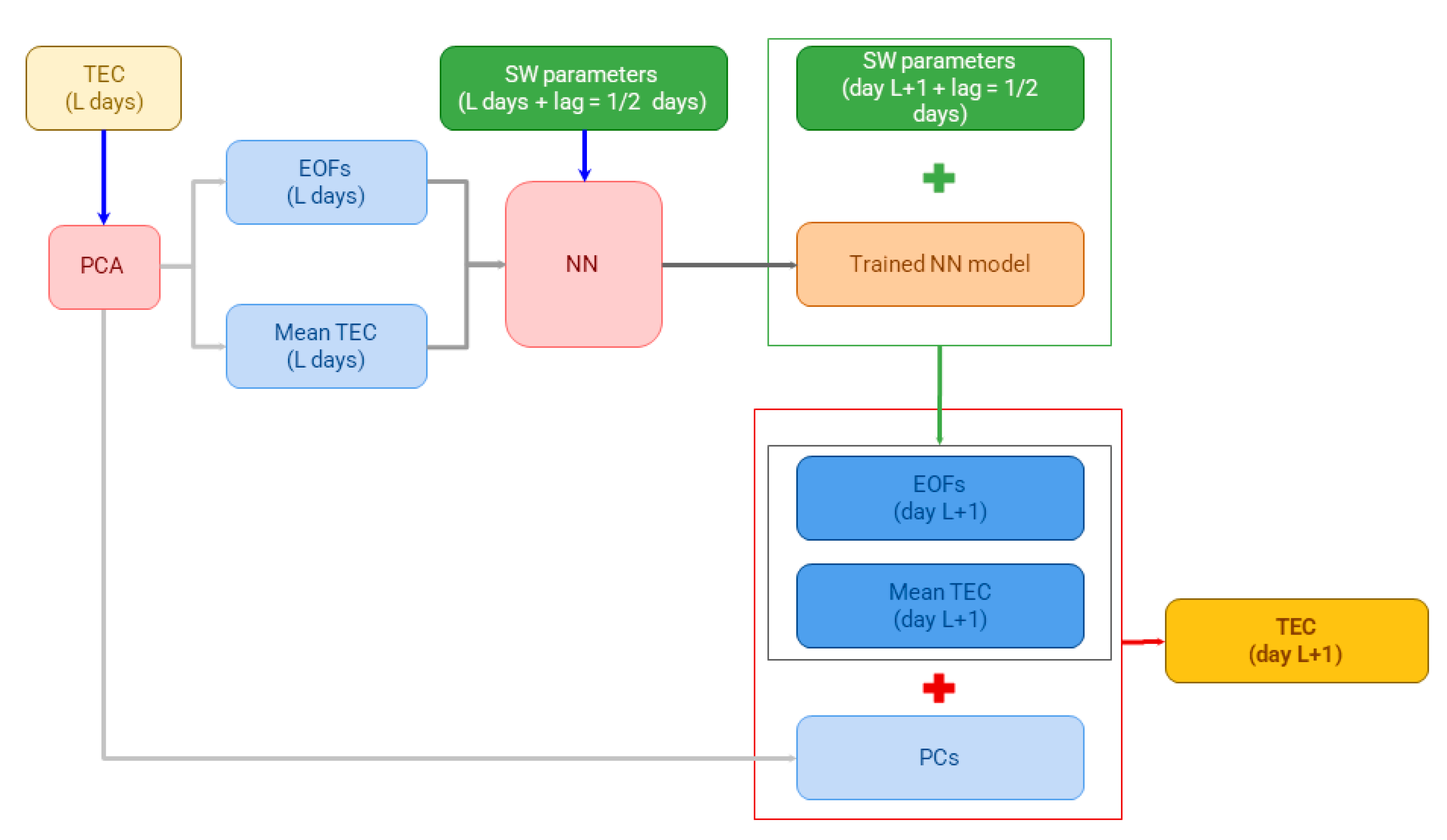
- A series of TEC of the length of 31 days with 1 h time resolution is decomposed by the principal component analysis (PCA) into daily modes;
- NN models are built to forecast the daily mean TEC and the amplitudes of the first two PCA modes using the lagged SWp. These NN models are used to forecast the daily mean TEC and the amplitudes of the first two PCA modes, and as a result the 1 h TEC series, for the following day.
Supplementary Materials
Author Contributions
Funding
Institutional Review Board Statement
Informed Consent Statement
Data Availability Statement
Acknowledgments
Conflicts of Interest
References
- Kumar, V.V.; Parkinson, M.L. A global scale picture of ionospheric peak electron density changes during geomagnetic storms. Space Weather 2017, 15, 637–652. [Google Scholar] [CrossRef]
- Tang, R.; Zeng, F.; Chen, Z.; Wang, J.S.; Huang, C.M.; Wu, Z. The comparison of predicting storm-time ionospheric TEC by three methods: ARIMA, LSTM, and Seq2Seq. Atmosphere 2020, 11, 316. [Google Scholar] [CrossRef]
- Xiong, P.; Zhai, D.; Long, C.; Zhou, H.; Zhang, X.; Shen, X. Long short-term memory neural network for ionospheric total electron content forecasting over China. Space Weather 2021, 19, e2020SW002706. [Google Scholar] [CrossRef]
- Sivavaraprasad, G.; Mallika, I.L.; Sivakrishna, K.; Ratnam, D.V. A novel hybrid Machine learning model to forecast ionospheric TEC over Low-latitude GNSS stations. Adv. Space Res. 2022, 69, 1366–1379. [Google Scholar] [CrossRef]
- Nath, S.; Chetia, B.; Kalita, S. Ionospheric TEC prediction using hybrid method based on ensemble empirical mode decomposition (EEMD) and long short-term memory (LSTM) deep learning model over India. Adv. Space Res. 2023, 71, 2307–2317. [Google Scholar] [CrossRef]
- Morozova, A.L.; Barata, T.; Barlyaeva, T. PCA-MRM model to forecast TEC at middle latitudes. Atmosphere 2022, 13, 323. [Google Scholar] [CrossRef]
- Iluore, K.; Lu, J. Long short-term memory and gated recurrent neural networks to predict the ionospheric vertical total electron content. Adv. Space Res. 2022, 70, 652–665. [Google Scholar] [CrossRef]
- Ren, X.; Yang, P.; Liu, H.; Chen, J.; Liu, W. Deep learning for global ionospheric TEC forecasting: Different approaches and validation. Space Weather 2022, 20, e2021SW003011. [Google Scholar] [CrossRef]
- Barlyaeva, T.; Barata, T.; Morozova, A. Datasets of ionospheric parameters provided by SCINDA GNSS receiver from Lisbon airport area. Data Brief 2020, 31, 105966. [Google Scholar] [CrossRef]
- Morozova, A.; Barlyaeva, T.; Barata, T. Datasets of ionospheric parameters (TEC, SI, positioning errors) from Lisbon airport area for 2014–2019. Data Brief 2023, 47, 109026. [Google Scholar] [CrossRef]
- Barlyaeva, T.; Barata, T.; Morozova, A. Datasets of ionospheric parameters provided by SCINDA GNSS receiver from Lisbon airport area. Mendeley Data 2020, 31, 105966. [Google Scholar] [CrossRef]
- Morozova, A.; Barlyaeva, T.; Barata, T. Datasets of ionospheric parameters (TEC, SI, positioning errors) from Lisbon airport area for 2014–2019. Mendeley Data 2022. [Google Scholar] [CrossRef]
- Morozova, A.L.; Barlyaeva, T.V.; Barata, T. Variations of TEC over Iberian Peninsula in 2015 due to geomagnetic storms and solar flares. Space Weather 2020, 18, e2020SW002516. [Google Scholar] [CrossRef]
- Yasyukevich, Y.V.; Mylnikova, A.A.; Kunitsyn, V.E.; Padokhin, A.M. Influence of GPS/GLONASS differential code biases on the determination accuracy of the absolute total electron content in the ionosphere. Geomagn. Aeron. 2015, 55, 763–769. [Google Scholar] [CrossRef]
- Mylnikova, A.A.; Yasyukevich, Y.V.; Kunitsyn, V.E.; Padokhin, A.M. Variability of GPS/GLONASS differential code biases. Results Phys. 2015, 5, 9–10. [Google Scholar] [CrossRef]
- Yasyukevich, Y.V.; Mylnikova, A.A.; Polyakova, A.S. Estimating the total electron content absolute value from the GPS/GLONASS data. Results Phys. 2015, 5, 32–33. [Google Scholar] [CrossRef]
- Morozova, A.L.; Ribeiro, P.; Blanco, J.J.; Barlyaeva, T.V. Temperature and pressure variability in mid-latitude low atmosphere and stratosphere-ionosphere coupling. Adv. Space Res. 2020, 65, 2184–2202. [Google Scholar] [CrossRef]
- Viereck, R.; Puga, L.; McMullin, D.; Judge, D.; Weber, M.; Tobiska, W.K. The Mg II index: A proxy for solar EUV. Geophys. Res. Lett. 2001, 28, 1343–1346. [Google Scholar] [CrossRef]
- Snow, M.; Weber, M.; Machol, J.; Viereck, R.; Richard, E. Comparison of Magnesium II core-to-wing ratio observations during solar minimum 23/24. J. Space Weather Space Clim. 2014, 4, A04. [Google Scholar] [CrossRef]
- Newell, P.T.; Sotirelis, T.; Liou, K.; Meng, C.-I.; Rich, F.J. A nearly universal solar wind-magnetosphere coupling function inferred from 10 magnetospheric state variables. J. Geophys. Res. 2007, 112, A01206. [Google Scholar] [CrossRef]
- Verkhoglyadova, O.P.; Komjathy, A.; Mannucci, A.J.; Mlynczak, M.G.; Hunt, L.A.; Paxton, L.J. Revisiting ionosphere-thermosphere responses to solar wind driving in superstorms of November 2003 and 2004. J. Geophys. Res. Space Phys. 2017, 122, 10–824. [Google Scholar] [CrossRef]
- Maruyama, T. Solar proxies pertaining to empirical ionospheric total electron content model. J. Geophys. Res. 2010, 115, A04306. [Google Scholar] [CrossRef]
- Mukhtarov, P.; Andonov, B.; Pancheva, D. Empirical model of TEC response to geomagnetic and solar forcing over Balkan Peninsula. J. Atmos. Sol. Terr. Phys. 2018, 167, 80–95. [Google Scholar] [CrossRef]
- Bjornsson, H.; Venegas, S.A. A Manual for EOF and SVD Analyses of Climatic Data; McGill University: Montreal, QC, Canada, 1997; CCGCR Report 97-1. [Google Scholar]
- Hannachi, A.; Jolliffe, I.T.; Stephenson, D.B. Empirical orthogonal functions and related techniques in atmospheric science: A review. Int. J. Climatol. 2007, 27, 1119–1152. [Google Scholar] [CrossRef]
- Shlens, J. A tutorial on principal component analysis. arXiv 2014, arXiv:1404.1100. [Google Scholar]
- Ebisuzaki, W. A method to estimate the statistical significance of a correlation when the data are serially correlated. J. Clim. 1997, 10, 2147–2153. [Google Scholar] [CrossRef]
- Sheskin, D.J. Handbook of Parametric and Nonparametric Statistical Procedures; Chapman and Hall/CRC: Boca Raton, FL, USA, 2003. [Google Scholar]
- Günther, F.; Fritsch, S. Neuralnet: Training of neural networks. R J. 2010, 2, 30. [Google Scholar] [CrossRef]
- Fritsch, S.; Guenther, F.; Guenther, M.F.; Package ‘neuralnet’. Training of Neural Networks. 2019. Available online: https://cran.r-project.org/web/packages/neuralnet/neuralnet.pdf. (accessed on 18 June 2023).
- Ciaburro, G.; Venkateswaran, B. Neural Networks with R: Smart models using CNN, RNN, Deep Learning, and Artificial Intelligence Principles; Packt Publishing Ltd.: Birmingham, UK, 2017. [Google Scholar]
- Barata, T.; Pereira, J.; Hernández-Pajares, M.; Barlyaeva, T.; Morozova, A. Ionosphere over Eastern North Atlantic Midlatitudinal Zone during Geomagnetic Storms. Atmosphere 2023, 14, 949. [Google Scholar] [CrossRef]
- Cherniak, I.; Zakharenkova, I. First observations of super plasma bubbles in Europe. Geophys. Res. Lett. 2016, 43, 11137–11145. [Google Scholar] [CrossRef]
- Bergeot, N.; Chevalier, J.-M.; Bruyninx, C.; Pottiaux, E.; Aerts, W.; Baire, Q.; Legrand, J.; Defraigne, P.; Huang, W. Near real-time ionospheric monitoring over Europe at the Royal Observatory of Belgium using GNSS data. J. Space Weather Space Clim. 2014, 4, A31. [Google Scholar] [CrossRef]
- Papitashvili, N.; King, J.H. May. Solar Wind Spatial Scales in, and Comparisons of, Hourly Wind and ACE IMF and Plasma Data. In AGU Spring Meeting Abstracts; American Geophysical Union: Washington, DC, USA, 2004; p. SH41A–07. [Google Scholar]


| Location | Latitude | Longitude |
|---|---|---|
| SCINDA (Lisbon) | 38.7° N | 9.14° W |
| Cascais | 38.7° N | 9.4° W |
| Furnas (Azores) | 37.8° N | 25.3° W |
| Funchal (Madeira) | 32.7° N | 16.9° W |
| Metrics | Time Resolution | Hours | PCA-MRM (2015 Only) | PCA-NN (2014–2018) |
|---|---|---|---|---|
| r (TECfor vs. TECobs) | 1 h | all | 0.89 | 0.92 |
| 1 d mean | – | 0.88 | 0.94 | |
| RMSE, TECu | 1 h | all | 4.3 | 2.7 |
| all (daily means) | 3.7 | 2.7 | ||
| day (daily means) | 4.5 | 3.3 | ||
| night (daily means) | 2.4 | 2.0 | ||
| 1 d mean | – | 2.8 | 1.7 | |
| MAE, TECu | 1 h | all | 2.9 | 1.9 |
| all (daily means) | 2.9 | 1.9 | ||
| day (daily means) | 3.9 | 2.3 | ||
| night (daily means) | 2.0 | 1.5 | ||
| 1 d mean | – | 2.0 | 1.2 | |
| MaxE, TECu | 1 h | all | 44.7 | 35.3 |
| 1 d mean | – | 15.3 | 13.6 | |
| ExpV | 1 h | all | 0.78 | 0.85 |
| 1 d mean | – | 0.77 | 0.89 | |
| R2 | 1 h | all | 0.80 | 0.85 |
| 1 d mean | – | 0.77 | 0.89 | |
| 90% confidence level, TECu | 1 h | all | ±5.0 | ±4.0 |
| day (daily means) | ±6.0 | ±4.8 | ||
| night (daily means) | ±3.0 | ±3.2 |
| Days | Hours | PCA-MRM | PCA-NN |
|---|---|---|---|
| Quiet | day (daily means) | 3.4 | 1.9 |
| night (daily means) | 2.0 | 1.4 | |
| With flares | day (daily means) | 3.6 | 2.4 |
| night (daily means) | 2 | 1.6 | |
| With geomagnetic storms without flares | day (daily means) | 8.8 | 4.5 |
| night (daily means) | 2.4 | 2.0 | |
| With flares and/or storms | day (daily means) | 4.4 | 2.6 |
| night (daily means) | 2.1 | 1.6 |
| TEC Parameter | PCA-MRM (Most Often Used) | PCA-NN (Best Forecasting Skills) |
|---|---|---|
| daily mean TEC | Mg II Dst XR By | Mg II Dst AE ap XR C.f. Daily mean TEC (lagged) |
| EOF1 | Mg II Dst AE By | Mg II Dst AE EOF1 (lagged) |
| EOF2 | Mg II Dst ap Bz p | F10.7 Dst AE (v) EOF2 (lagged) |
| Daily Mean TEC, TECu | EOF1, arb. u. | EOF2, arb. u. | |
|---|---|---|---|
| NN (nodes per hidden layer) | (14,6,4) | (8,6,4) | (8,6,4) |
| Number of predictors | 7 predictors | 4 predictors | 4 predictors |
| SWp predictors | MgII Dst C.f. ap AE XR daily mean TEC | AE MgII Dst EOF1 | AE Dst F10.7 EOF2 |
| R | 0.94 | 0.35 | 0.47 |
| MAE | 1.19 | 0.05 | 0.12 |
| RMSE | 1.72 | 0.07 | 0.16 |
| Metrics | SCINDA (Lisbon) | Cascais | Furnas (Azores) | Funchal (Madeira) |
|---|---|---|---|---|
| r(TECfor vs. TECobs), 2015 & 2017–2018 | 0.93 | 0.94 | 0.94 | 0.93 |
| r(TECfor vs. TECobs), 2015 | 0.90 | 0.88 | 0.88 | 0.83 |
| r(TECfor vs. TECobs), 2017–2018 | 0.80 | 0.88 | 0.88 | 0.89 |
| 95% confidence level, TECu | ±5.0 | ±5.5 | ±5.0 | ±8.5 |
| 90% confidence level, TECu | ±4.0 | ±4.0 | ±3.5 | ±6.0 |
| MAPE | 0.18 | 0.19 | 0.16 | 0.29 |
Disclaimer/Publisher’s Note: The statements, opinions and data contained in all publications are solely those of the individual author(s) and contributor(s) and not of MDPI and/or the editor(s). MDPI and/or the editor(s) disclaim responsibility for any injury to people or property resulting from any ideas, methods, instructions or products referred to in the content. |
© 2023 by the authors. Licensee MDPI, Basel, Switzerland. This article is an open access article distributed under the terms and conditions of the Creative Commons Attribution (CC BY) license (https://creativecommons.org/licenses/by/4.0/).
Share and Cite
Morozova, A.; Barata, T.; Barlyaeva, T.; Gafeira, R. Total Electron Content PCA-NN Prediction Model for South-European Middle Latitudes. Atmosphere 2023, 14, 1058. https://doi.org/10.3390/atmos14071058
Morozova A, Barata T, Barlyaeva T, Gafeira R. Total Electron Content PCA-NN Prediction Model for South-European Middle Latitudes. Atmosphere. 2023; 14(7):1058. https://doi.org/10.3390/atmos14071058
Chicago/Turabian StyleMorozova, Anna, Teresa Barata, Tatiana Barlyaeva, and Ricardo Gafeira. 2023. "Total Electron Content PCA-NN Prediction Model for South-European Middle Latitudes" Atmosphere 14, no. 7: 1058. https://doi.org/10.3390/atmos14071058
APA StyleMorozova, A., Barata, T., Barlyaeva, T., & Gafeira, R. (2023). Total Electron Content PCA-NN Prediction Model for South-European Middle Latitudes. Atmosphere, 14(7), 1058. https://doi.org/10.3390/atmos14071058