Comprehensive Analysis of the Global Zenith Tropospheric Delay Real-Time Correction Model Based GPT3

Abstract

To obtain a higher accuracy for the real-time Zenith Tropospheric Delay (ZTD), a refined tropospheric delay correction model was constructed by combining the tropospheric delay correction model based on meteorological parameters and the GPT3 model. The meteorological parameters provided by the Global Geodetic Observing System (GGOS) Atmosphere and the zenith tropospheric delay data provided by Centre for Orbit Determination in Europe (CODE) were used as references, and the accuracy and spatial–temporal characteristics of the proposed model were compared and studied. The results show the following: (1) Compared with the UNB3m, GPT and GPT2w models, the accuracy and stability of the GPT3 model were significantly improved, especially the estimation accuracy of temperature, the deviation (Bias) of the estimated temperature was reduced by 90.60%, 32.44% and 0.30%, and the root mean square error (RMS) was reduced by 42.40%, 11.02% and 0.11%, respectively. (2) At different latitudes, the GPT3 + Saastamoinen, GPT3 + Hopfield and UNB3m models had great differences in accuracy and applicability. In the middle and high latitudes, the Biases of the GPT3 + Saastamoinen model and the GPT3 + Hopfield model were within 0.60 cm, and the RMS values were within 4 cm; the Bias of the UNB3m model was within 2 cm, and the RMS was within 5 cm; in low latitudes, the accuracy and stability of the GPT3 + Saastamoinen model were better than those of the GPT3 + Hopfield and UNB3m models; compared with the GPT3 + Hopfield model, the Bias was reduced by 22.56%, and the RMS was reduced by 5.67%. At different heights, the RMS values of the GPT3 + Saastamoinen model and GPT3 + Hopfield model were better than that of the UNB3m model. When the height was less than 500 m, the Biases of the GPT3 + Saastamoinen, GPT3 + Hopfield and UNB3m models were 3.46 cm, 3.59 cm and 4.54 cm, respectively. At more than 500 m, the Biases of the three models were within 4 cm. In different seasons, the Bias of the ZTD estimated by the UNB3m model had obvious global seasonal variation. The GPT3 + Saastamoinen model and the GPT3 + Hopfield model were more stable, and the values were within 5 cm. The research results can provide a useful reference for the ZTD correction accuracy and applicability of GNSS navigation and positioning at different latitudes, at different heights and in different seasons.

1. Introduction

Zenith Tropospheric Delay (ZTD) is one of the main error sources of high-precision positioning of global navigation satellite system (GNSS) [1], and it is also an important data source for GNSS space environment research [2,3,4]. The slant total delay (STD) can reach 20 m at a 5° cutoff angle, which was derived from the mapping function (such as the Niell Mapping Function (NMF) [5], the Global Mapping Function (GMF) [6] and the Vienna Mapping Function (VMF1) [7]) and ZTD. Therefore, it is particularly important to establish a high-precision tropospheric delay correction model. The commonly used tropospheric delay correction models can be divided into two types: one is the tropospheric delay correction model based on meteorological parameters, and the other is the tropospheric delay correction model without meteorological parameters [8]. The Saastamoinen model, Hopfield model and Black model are widely used models based on measured meteorological parameters [9,10,11]. Experimental results have shown that the tropospheric zenith delay correction accuracy based on the meteorological parameter model is high (although there may be slight differences under different conditions), with the correction accuracy able to reach the centimeter level [12]. These models require measured meteorological parameters as inputs, therefore greatly limiting the use of such models. Therefore, non-meteorological parameter models have become a research hotspot. Currently, the commonly used models without meteorological parameters are the University of New Brunswick (UNB) model [13] established by Collins and Langley, the European Geostationary Navigation Overlay Service [14] (EGNOS) and the Global Pressure and Temperature (GPT) model [15] established by Boehm et al. With the continuous development and improvement of the UNB series models, the UNB3m improved the estimation of wet delay and reduced the Bias to −0.5 cm [16]. Huang et al. [17] established the Single-Site Improved EGNOS (SS-IEGNOS) model in Asia, and the accuracy and applicability of the EGNOS and SS-IEGNOS models were evaluated. The results indicated that the Bias and root mean square error (RMS) of the EGNOS model showed obvious seasonal variation in time distribution, while the Bias and RMS of the SS-IEGNOS model changed little and smoothly. To date, the GPT series models have gradually produced GPT2, GPT2w and GPT3 models from the initial GPT model. To evaluate the accuracy of the above model, scholars have also carried out a lot of experimental verification; Wang et al. [18] analyzed the accuracy of the EGNOS, UNB3m, GPT and GPT2 models in China using the measured data from 223 stations in the land state network of the Shanghai Observatory. The results showed that the RMS values of the four models were 4−5 cm, and the RMS value of the GPT2 model was the smallest. The average Bias of the four models was about 1 cm, and the maximum Bias of the GPT2 model was 1.5 cm; Zhu et al. [19] used the meteorological upper-air observation data in China to analyze the accuracy of temperature (T), weighted average temperature (Tm), pressure (P) and water vapor pressure (e) of the GPT2w model, which provided a basis for improving the application accuracy of the model in China. Gao et al. [20] verified the accuracy of the GPT3 model in China. The experimental results demonstrated that the GPT3 model was comparable to the GPT2w model, but the stability was improved. Due to the special geographical location of the Antarctic, the meteorological conditions are different from other locations on the Earth. Kong et al. [21] analyzed the accuracy of the GPT2w model in the Antarctic region. The results showed that the accuracy of the model near the ground was consistent with that of other regions in the world, but with an increase in height, the Bias and RMS would also increase, and the accuracy would decrease. To improve the accuracy of the GPT2w model, Yang et al. [22] established an improved GPT2w model based on a BP (Back Propagation) neural network, which was nearly 32% higher than the GPT2w model. Li et al. [23] established an improved GPT3 model LSTM _ RBF _ ZTD model based on long short-term memory (LSTM) and radial basis function (RBF) neural network coupling, and they analyzed the accuracy of the model in the Antarctic. The experimental results show that the accuracy of the LSTM _ RBF _ ZTD model was 39.6% higher than that of the GPT3 _ ZTD in 65 stations. In conclusion, the GPT3 model is widely used, but it cannot provide vertical profile information of ZTD. In recent years, the tropospheric vertical profile function has been widely studied by many scholars [24,25]. Zhu et al. [26] developed an ERA5-based global model for the vertical adjustment of zenith tropospheric delay using a piecewise function; the results show that the performance of the Global Zenith Tropospheric Delay Piecewise (GZTD-P) model was improved by 0.96 cm (23%) relative to the GPT3 mode.

To improve the correction accuracy of ZTD, the meteorological model that is most consistent with the actual meteorological parameters is usually selected [27]. Yang et al. [28] used the temperature and pressure obtained by the GPT model and the water vapor pressure obtained by the UNB3m model as the input parameters of the Saastamoinen model to construct a comprehensive, improved tropospheric delay model, which has wider applicability. Yao et al. [29] used the meteorological parameters provided by the GPT2 model and the Saastamoinen model to calculate the ZTD and constructed a tropospheric delay correction model suitable for the global scale. The above improved models were all established global tropospheric delay models. Aiming at the accuracy requirements of the improved tropospheric delay model in the local range, Yang et al. [30] proposed a method to increase the annual period and half-year period on the basis of the Hopfield model. The GHop model adapted to the Chinese region was established using the least squares fitting method. The model had higher accuracy and adaptability than the Hopfield model in latitude and height. Focusing on the problem that the tropospheric delay correction is limited by the real-time and poor practicability of sounding data, Du et al. [31] used the ZTD time series of the International GNSS Service (IGS) stations and the meteorological data from stations published by the Global Geodetic Observing System (GGOS) to verify the GPT2w + Saastamoinen model. The experiments showed that the accuracy of the GPT2w + Saastamoinen model was better than that of the other combined models (Saastamoinen + EGNOS model, Saastamoinen + UNB3m model and GPT2w + Hopfield model) under the same conditions. Liu et al. [32] proposed a data fusion tropospheric delay estimation method. The dry delay was estimated by the Saastamoinen model, and the wet delay was obtained by the Askne model. The accuracy of this method was 8.10 mm higher than that of the GPT2w + Saastamoinen model. Yang et al. [33] used ERA5 data and global distributed sounding data to evaluate the performance of the improved Saastamoinen model. The numerical results showed that the improved model was better than the Saastamoinen model and the improved Bias and RMS were 0.54 and 2.08 mm, respectively.

Although many tropospheric delay correction models have been constructed, there are few studies that have systematically investigated and compared the error characteristics of the GPT3 model, and there is a lack of in-depth discussion on the accuracy and applicability of the refined GPT3 + Saastamoinen/Hopfield model. In this study, the accuracy and seasonal variation characteristics of the GPT3 model were systematically evaluated. On this basis, a refined GPT3 + Saastamoinen/Hopfield model was established. The ZTD products provided by the Centre for Orbit Determination in Europe (CODE) were used as reference values to verify the accuracy and spatial and temporal distribution characteristics of the model at different latitudes, different heights and in different seasons.

The structure of the manuscript is summarized as follows. Section 2 introduces the theory of tropospheric delay models based on non-measured meteorological parameters—the UNB3m model and GPT series model—and evaluates the function of meteorological parameters estimated by the UNB3m, GPT, GPT2w and GPT3 models. The UNB3m, GPT3 + Saastamoinen and GPT3 + Hopfield models are compared and analyzed from three aspects of latitude, height and season in Section 3. Section 4 discusses the advantages of this work. Finally, the conclusion is given in Section 5.

2. Tropospheric Delay Correction Model Based on Non-Measured Meteorological Data

2.1. Methodology and Model

This type of model obtains the required meteorological parameters by extrapolation or interpolation according to the day of the year (Doy) and station position, and then calculates the tropospheric delay using the physical model [34].

2.1.1. UNB3m Model

The UNB3m model considers the annual period and annual amplitude of meteorological parameters and uses a latitude interval of 15° to represent various meteorological elements (pressure (P), temperature (T), relative humidity (RH), temperature change rate and water vapor pressure (e) change rate). The meteorological parameters are shown in

Table 1. Annual average of meteorological parameters.

Latitude (°)	P (hPa)	T (K)	RH (%)	T Change Rate (K/m)	e Change Rate
15	1013.25	299.65	75.0	0.00630	2.77
30	1017.25	294.15	80.0	0.00605	3.15
45	1015.75	283.15	76.0	0.00558	2.57
60	1011.75	272.15	77.5	0.00539	1.81
75	1013.00	263.65	82.5	0.00453	1.55

and

Table 2. Annual amplitude values of meteorological parameters.

Latitude (°)	P (hPa)	T (K)	RH (%)	T Change Rate (K/m)	e Change Rate
15	0.00	0.00	0.0	0.00	0.00
30	−3.75	7.00	0.0	0.00025	0.33
45	−2.25	11.00	−1.0	0.00032	0.46
60	−1.75	15.00	−2.5	0.00081	0.74
75	−0.50	14.50	2.5	0.00062	0.30

:

The annual average $av{g}_{\mathit{\varphi }}$ and annual periodic amplitude $am{p}_{\mathit{\varphi }}$ can be calculated using linear interpolation according to the latitude of the station. The interpolation equation is as follows:

$$av{g}_{\mathit{\varphi }}=\left\{\begin{array}{l}av{g}_{15}\mathit{if} \mathit{\varphi }\le 15\\ av{g}_{75}\mathit{if} \mathit{\varphi }\ge 75\\ av{g}_i+\frac{(av{g}_{i+1}-av{g}_i)}{15}(\mathit{\varphi }-la{t}_i) \mathit{if} 15\text{<}\mathit{\varphi }<75 \end{array}\right.$$

(1)

$$am{p}_{\mathit{\varphi }}=\left\{\begin{array}{l}am{p}_{15}\mathit{if} \mathit{\varphi }\le 15\\ am{p}_{75}\mathit{if} \mathit{\varphi }\ge 75\\ am{p}_i+\frac{(am{p}_{i+1}-am{p}_i)}{15}(\mathit{\varphi }-la{t}_i) \mathit{if} 15\text{<}\mathit{\varphi }<75 \end{array}\right.$$

(2)

In the equation, i is the index value of the latitude that is the nearest to the station and lower than the latitude of the station and $la{t}_i$ is the latitude value of the index.

According to the annual averages and annual periodic amplitudes of the meteorological parameters, the meteorological parameters are calculated using Equation (3).

$$X_{\mathit{\varphi },doy}=av{g}_{\mathit{\varphi }}-am{p}_{\mathit{\varphi }}\cdot \cos \left(\right(doy-28)\frac{2\mathsf{\pi }}{365.25})$$

(3)

According to the meteorological parameters, the dry delay and wet delay can be obtained as follows, where zpd represents the dry delay and zpw represents the wet delay:

$$\left\{\begin{array}{l}{\mathit{\delta }}_{\mathrm{zpd}}=\frac{{10}^{-6}{k}_{1}R}{g_{\mathrm{m}}}P{(1-\frac{\mathit{\beta }H}{T})}^{\frac{g}{R\mathit{\beta }}}\\ {\mathit{\delta }}_{\mathrm{zpw}}=\frac{{10}^{-6}(T_m{K}_2+K_3)R}{g_{\mathrm{m}}(\mathit{\lambda }+1)-\mathit{\beta }R}\frac{e}{T}{(1-\frac{\mathit{\beta }H}{T})}^{\frac{g(\mathsf{\lambda }+1)}{R\mathsf{\beta }}-1}\end{array}\right.$$

(4)

where g is the standard gravity acceleration (9.80665 m/s²); H is the height (m); $k_1,k_2,k_3$ are the refractivity constants; R is the dry atmospheric gas constant (287.054 J kg⁻¹ K⁻¹); $g_m$ is the gravity acceleration of the cylinder atmosphere; $T_m$ is the weighted average temperature; $\mathit{\beta }$ is the temperature lapse rate; and $\mathit{\lambda }$ is the water vapor pressure height factor. The calculation equation is as follows:

$$\left\{\begin{array}{l}{g}_m=9.784(1-0.00266\cos (2\mathit{\varphi })-2.8\times {10}^{-7}H)\\ T_m=(T-\mathit{\beta }H)(1-\frac{\mathit{\beta }R}{g_m(\mathit{\lambda }+1)})\end{array}\right.$$

(5)

The relative humidity RH is required to calculate the water vapor pressure e of UNB3m; the calculation equation is as follows:

$$\left\{\begin{array}{l}e=\frac{RH}{100}\cdot e_s\cdot f_w\\ e_{\mathrm{s}}=0.01\times \exp (1.2378847\times {10}^{-5}{T}^2-1.9121316\times {10}^{-2}T\\ +33.93711047-6.3431645\times {10}^3{T}^{-1})\\ f_w=1.00062+3.14\times {10}^{-6}P+5.6\times {10}^{-7}\cdot {(T-273.15)}^2\end{array}\right.$$

(6)

2.1.2. GPT Series Model

The GPT model uses the global temperature and pressure grid data with a resolution of $15°\times 15°$ provided by the European Centre for Medium-range Weather Forecasts (ECMWF). By inputting the location and time information of the station, the temperature and pressure at any location in the world can be obtained. However, the initial phase of the model is fixed on 28 January, only the average period and annual period are considered and the fixed temperature attenuation rate and the pressure change rate constructed by the standard atmosphere are used. Therefore, the horizontal resolution and time resolution are low and the error is large. On this basis, the GPT2 model was established based on the global monthly meteorological data from 2001 to 2010 provided by ERA-Interim [35]. The model provides parameters such as pressure, atmosphere temperature and water vapor pressure and attenuation rate with a resolution of $5°\times 5°$. At the same time, the model also considers the amplitude of various meteorological parameters and uses trigonometric functions to estimate various meteorological parameters. The model is shown in Equation (7).

$$\begin{array}{c}r(t)=A_0+A_1\cos \left(\frac{doy}{365.25}2\mathsf{\pi }\right)+B_1\sin \left(\frac{doy}{365.25}2\mathsf{\pi }\right)\\ +A_2\cos \left(\frac{doy}{365.25}4\mathsf{\pi }\right)+B_2\sin \left(\frac{doy}{365.25}4\mathsf{\pi }\right)\end{array}$$

(7)

In the equation, $r(t)$ is the estimated meteorological parameter; $doy$ is the day of the year; $A_0$ is the annual average amplitude; $A_1$ and $B_1$ are annual period parameters; and $A_2$ and $B_2$ are half-year period parameters. This model requires inputting the geodetic coordinates of the station and the modified Julian date, finding the nearest four grid points according to the coordinates, calculating the corresponding meteorological parameters of the four grid points using Equation (7) and then calculating the meteorological data at the grid points according to the height of the station. The other positions are interpolated by bilinear interpolation to obtain the meteorological data. Based on the GPT2 model, the GPT2w model adds the atmospheric weighted temperature and water vapor attenuation factor [36].

The number of meteorological parameters of the GPT3 model is consistent with that of GPT2w, and the modeling data is the same as that of the GPT2 model. The advantage of the GPT3 model is that the two parameters of atmospheric weighted average temperature and water vapor pressure lapse rate are added [37], and their parameters are substituted into the Askne and Nordius equation in Reference [38] to calculate the wet delay. The equation for calculating meteorological parameters in this model is as follows:

$$\begin{array}{c}r(t)=A_0+A_1\cos \left(\frac{2\mathsf{\pi }t}{365.25}\right)+B_1\sin \left(\frac{2\mathsf{\pi }t}{365.25}\right)\\ +A_2\cos \left(\frac{4\mathsf{\pi }t}{365.25}\right)+B_2\sin \left(\frac{4\mathsf{\pi }t}{365.25}\right)\end{array}$$

(8)

2.2. Model Accuracy Test and Analysis

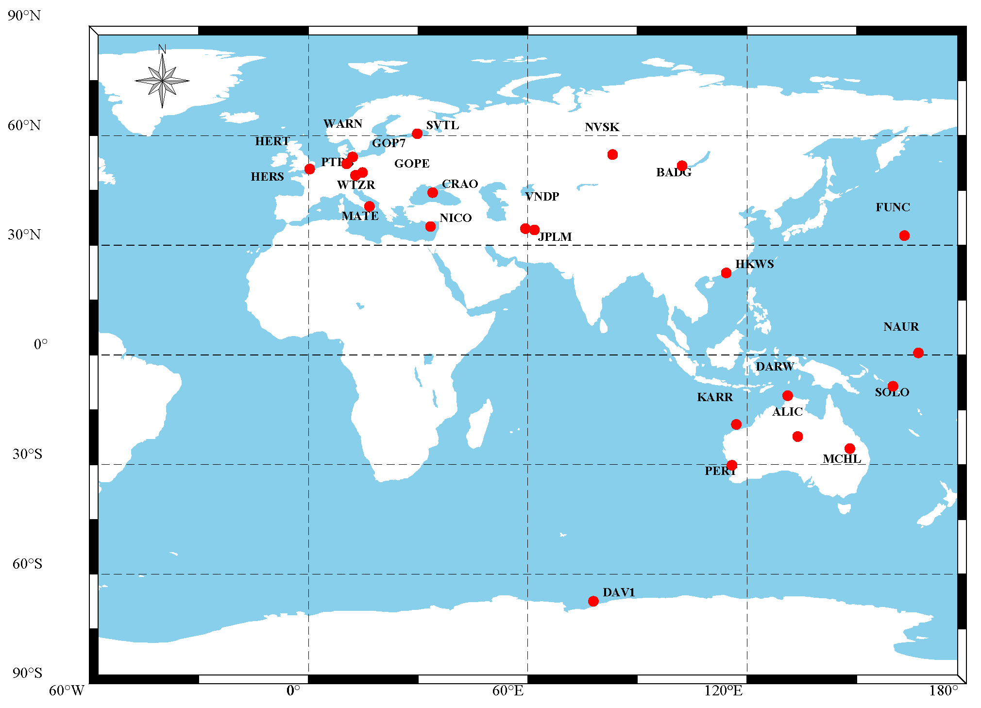
To analyze the accuracy of the tropospheric delay correction model without meteorological parameters at different latitudes, 25 stations were selected. Figure 1 describes the geographical distribution of the 25 IGS stations at different latitudes. Using the meteorological parameters provided by GGOS Atmosphere in 2018 as experimental reference values, the accuracy of the UNB3m, GPT, GPT2w and GPT3 models was analyzed. Due to the limited space of the manuscript, we only provided the comparison results for temperature, pressure and water vapor pressure at the DAV1 station in 2018, as shown in Figure 2. It can be seen from the figure that, whether it is temperature, pressure or water vapor pressure, the estimated results of the GPT series models were closer to the meteorological parameters provided by GGOS Atmosphere than the estimated results of the UNB3m model. For the GPT series models, the GPT2w and GPT3 models were better than the GPT model in estimating the pressure, and the estimation results of the three models were basically the same in terms of estimating the temperature and water vapor pressure.

To better quantitatively compare the deviation between the estimated value of the model and the reference value and the stability of the model, the Bias and RMS were used to evaluate the tropospheric delay accuracy of the various model corrections, and the Bias and RMS equations for calculating the meteorological parameters were as follows:

$$\left\{\begin{array}{l}\mathrm{Bias}=\frac{1}{N}{\displaystyle \sum _{i=1}^N(X_i^{\mathrm{Model}}-X_i^{\mathrm{GGOS}})}\\ \mathrm{RMS}=\sqrt{\frac{1}{N}{\displaystyle \sum _{i=1}^N{(X_i^{\mathrm{Model}}-X_i^{\mathrm{GGOS}})}^2}}\end{array}\right.$$

(9)

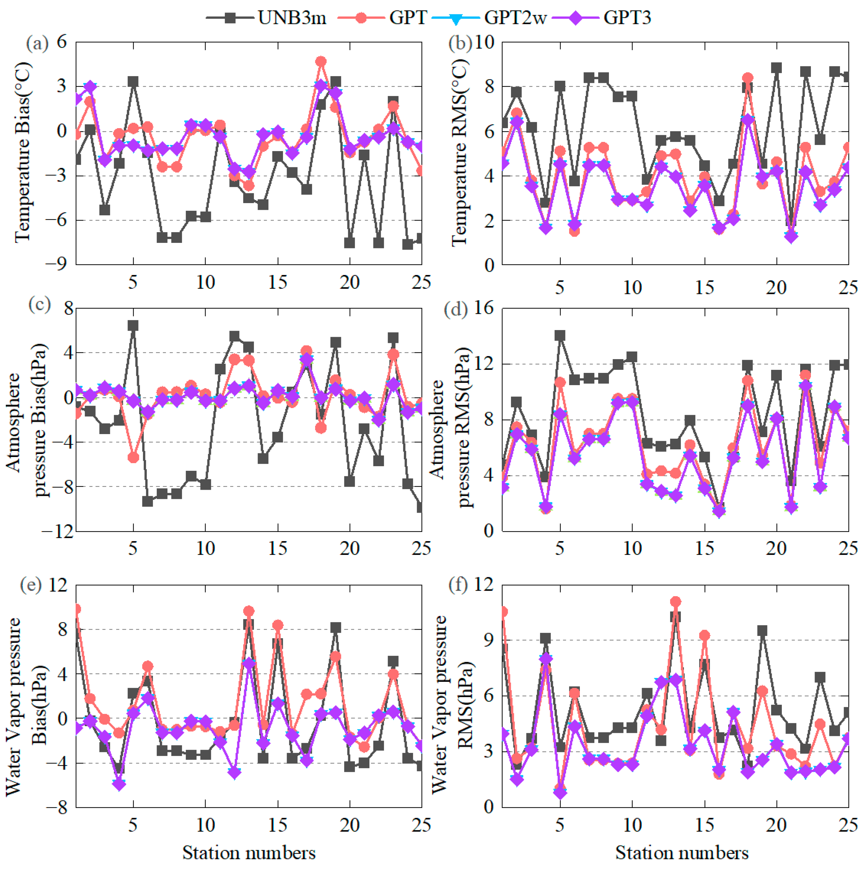
where $X_i^{\mathrm{GGOS}}$ is the meteorological parameter value provided for GGOS Atmosphere, $X_i^{\mathrm{Model}}$ is the calculated value of the model and N is the cumulative number of days.

Table 3. Temperature estimation results of 25 IGS stations using four non-measured meteorological parameter models (°C).

Num	Station	UNB3m		GPT		GPT2w		GPT3
		Bias	RMS	Bias	RMS	Bias	RMS	Bias	RMS
1	ALIC	−1.9135	6.3812	−0.2378	5.0517	2.1720	4.5427	2.1711	4.5453
2	BADG	0.0774	7.7311	1.9859	6.8018	2.9740	6.4437	2.9797	6.4063
3	CRAO	−5.3192	6.1551	−1.9585	3.8039	−1.9286	3.5680	−1.9280	3.5392
4	DARW	−2.1730	2.7925	−0.1580	1.6773	−0.9622	1.6752	−0.9623	1.6680
5	DAV1	3.3273	8.0115	0.1793	5.1030	−0.9523	4.5171	−0.9524	4.5191
6	FUNC	−1.4486	3.7521	0.2855	1.5156	−1.3100	1.8465	−1.3100	1.8343
7	GOP7	−7.1667	8.3848	−2.4108	5.2556	−1.1701	4.4718	−1.1709	4.4716
8	GOPE	−7.1669	8.3850	−2.4109	5.2559	−1.1703	4.4720	−1.1710	4.4718
9	HERS	−5.7303	7.5382	0.0806	2.9074	0.4348	2.9487	0.4350	2.9427
10	HERT	−5.7737	7.5787	0.0418	2.9115	0.4013	2.9461	0.4023	2.9394
11	HKWS	0.1832	3.8251	0.3964	3.2801	−0.3668	2.6812	−0.3669	2.6875
12	JPLM	−3.3499	5.5807	−2.9921	4.8943	−2.5178	4.4193	−2.5166	4.4192
13	KARR	−4.5061	5.7629	−3.6653	4.9741	−2.7412	3.9707	−2.7384	3.9613
14	MATE	−4.9673	5.5916	−1.0074	2.8735	−0.2070	2.4531	−0.2037	2.4414
15	MCHL	−1.7269	4.4583	−0.3177	3.9468	−0.0464	3.5745	−0.0464	3.5695
16	NAUR	−2.7698	2.8770	−1.3973	1.6017	−1.4776	1.6655	−1.4777	1.6658
17	NICO	−3.9122	4.5365	0.1308	2.2712	−0.3978	2.0856	−0.3981	2.0566
18	NVSK	1.7773	7.9484	4.6920	8.3886	3.0635	6.5085	3.0689	6.5070
19	PERT	3.3455	4.5352	1.6029	3.6308	2.5633	3.9595	2.5632	3.9585
20	PTBB	−7.5542	8.8320	−1.4543	4.6189	−1.1907	4.1951	−1.1896	4.1942
21	SOLO	−1.6028	1.9772	−0.7334	1.3533	−0.6111	1.2787	−0.6111	1.2772
22	SVTL	−7.5057	8.6615	0.1260	5.2755	−0.3919	4.1362	−0.3901	4.1615
23	VNDP	2.0020	5.6189	1.6683	3.2991	0.1723	2.6821	0.1723	2.6968
24	WARN	−7.6430	8.6589	−0.7599	3.7200	−0.7436	3.3568	−0.7436	3.3763
25	WTZR	−7.2297	8.4190	−2.6590	5.2725	−1.0297	4.3915	−1.0292	4.3848

only shows the temperature estimation results of the four models at 25 IGS stations. The estimation accuracy of the four models without meteorological parameters in the 25 IGS stations around the world is shown in Figure 3.

Table 3 and Figure 3 indicate that the accuracy of the GPT2w and GPT3 models was significantly improved compared to the UNB3m and GPT models. Among the 25 IGS stations, the temperature Biases of the GPT2w and GPT3 models were within −3 °C–3 °C, the Bias was −1.5 hPa–1.5 hPa and the Bias of water vapor pressure was within −3 hPa–3 hPa (except for the DARW, JPLM, KARR and NICO stations). At the same time, the stability of the GPT2w and GPT3 models was also improved compared with the UNB3m and GPT models. To further compare the accuracy of the four models,

Table 4. Annual mean Bias and RMS values of meteorological parameters in 2018 estimated by four models.

Meteorological Parameters	UNB3m		GPT		GPT2w		GPT3
	Bias	RMS	Bias	RMS	Bias	RMS	Bias	RMS
T (°C)	−3.1531	6.1597	−0.4389	3.9874	−0.2974	3.5516	−0.2965	3.5478
P (hPa)	−2.4055	8.4121	0.1501	6.2534	0.1109	5.6000	0.1107	5.5989
e (hPa)	−0.3366	5.1994	1.3165	4.3646	−0.8880	3.3807	−0.8876	3.3780

shows the annual mean deviation and RMS values for the four models without the estimation of meteorological parameters. The accuracy of the GPT series models was better than that of the UNB3m model; compared with the UNB3m, GPT and GPT2w models, the accuracy of the GPT3 model was the best: the estimation accuracy of temperature was more prominent, the temperature Bias was reduced by 90.60%, 32.44% and 0.30% and the temperature RMS was reduced by 42.40%, 11.02% and 0.11%, respectively (Table 4).

To explore the seasonal variation characteristics of the GPT3 model,

Table 5. Bias/RMS of temperature, pressure and water vapor pressure.

Month	T (°C)		P (hPa)		e (hPa)
	Bias	RMS	Bias	RMS	Bias	RMS
January–March	0.3280	3.8160	1.4779	7.0594	−0.6389	2.8166
April–June	−0.6943	3.3844	−0.3961	4.5565	−0.9901	3.4225
July–September	−0.5778	3.2926	−0.3896	4.0990	−1.0261	3.4697
October–December	−0.2227	3.4188	−0.2873	5.9322	−0.8882	3.4110

shows the statistical results of the Bias and RMS values during four seasons for temperature, pressure and water vapor pressure (the corresponding months of the four seasons are as follows: January–March, April–June, July–September and October–December). It can be seen from the table that in different seasons, the Bias and RMS values for temperature, pressure and water vapor pressure were quite different, indicating that there is obvious seasonality. In terms of temperature, the Bias was the smallest in October–December with a value of −0.2227 °C, followed by January–March, and the largest was observed for April–June; July–September had the best accuracy with an RMS value of 3.2926 °C, followed by April–June, and the worst was observed for January–March. In terms of pressure, the Bias was the smallest in October–December with a value of −0.2873 hPa, followed by July–September, and the largest was observed in January–March; July–September had the highest accuracy with an RMS of 4.0990 hPa, followed by April–June, and January–March was the worst. In terms of water vapor pressure, the accuracy was highest in January–March, with Bias and RMS values of −0.6389 hPa and 2.8166 hPa, respectively, followed by October–December, with the worst in July–September.

3. A High-Precision GNSS Tropospheric Zenith Delay Correction Model with GPT3 Fusion

3.1. Tropospheric Delay Correction Model Based on Meteorological Parameters

Currently, zenith tropospheric delay is mainly divided into dry delay and wet delay. For dry delay correction, the tropospheric delay correction model based on meteorological parameters has reached the millimeter level of accuracy. However, due to the uneven distribution of water vapor in the atmosphere and the complex changes over time, the tropospheric correction model based on meteorological parameters has relatively poor accuracy for wet component correction, and its zenith direction correction accuracy is generally at the centimeter level [39].

3.1.1. Hopfield Model

The tropospheric wet delay and dry delay calculated by the improved Hopfield model are as follows:

$${\mathit{\delta }}_i={10}^{-12}{N}_i[{\displaystyle \sum _{k=1}^9\frac{{\mathbf{\alpha }}_{k,i}}{k}{r}_i^k}]$$

(10)

where the subscript i can represent either the dry delay (replace i with zpd) or the wet delay (replace i with zpw) and $N_i$ denotes the atmospheric refractive index. The equation is as follows:

$$\left\{\begin{array}{l}{N}_{\mathrm{zpd}}=0.776\times \frac{{10}^{-4}P}{T}\\ N_{\mathrm{zpw}}=\frac{0.373e}{T^2}\end{array}\right.$$

(11)

where $T,P,e$ represent the temperature (K), atmospheric pressure (mbar) and water vapor pressure (mbar) of the station, respectively; r represents the distance from the station to the intersection of the propagation path and the boundary surface where the dry and wet refractivity tends to zero. The unit of r is m, and the calculation equation is

$$r_i=\sqrt{{(R+h_i)}^2-{\left(R\cos E\right)}^2}-R\sin E$$

(12)

where h is the height of the boundary surface where the dry and wet refractivity tends to zero and the unit is m. The calculation equation is as follows:

$$\left\{\begin{array}{l}{h}_{\mathrm{zpd}}=\mathrm{40,136}+148.72(T-273.16)\\ h_{\mathrm{zpw}}=\mathrm{11,000}\end{array}\right.$$

(13)

The coefficients ${\mathbf{\alpha }}_{k,i}$ in Equation (10) are expressed as follows:

$$\begin{array}{l}{\mathbf{\alpha }}_{1,i}=1,{\mathbf{\alpha }}_{2,i}=4a_i,{\mathbf{\alpha }}_{3,i}=6a_i^2+4b_i\\ {\mathbf{\alpha }}_{4,i}=4a_i(a_i^2+3b_i),{\mathbf{\alpha }}_{5,i}=a_i^4+12a_i^2{b}_i+6b_i^2,{\mathbf{\alpha }}_{6,i}=4a_i{b}_i(a_i^2+3b_i)\\ {\mathbf{\alpha }}_{7,i}=b_i^2(6a_i^2+4b_i),{\mathbf{\alpha }}_{8,i}=4a_i{b}_i^3{\mathbf{\alpha }}_{9,i}=b_i^4\end{array}$$

(14)

$$a_i=-\frac{\sin E}{h_i},b_i=-\frac{{\cos }^{2}E}{2h_{i}R}$$

(15)

In Equation (14), $E$ is the elevation angle of the satellite, in °, and R is the geocentric distance of the station, in km.

3.1.2. Saastamoinen Model

In the Saastamoinen model, the tropospheric wet and dry components are calculated as follows:

$$\mathrm{ZTD}={\mathit{\delta }}_{\mathrm{zpd}}+{\mathit{\delta }}_{\mathrm{zpw}}=\frac{0.002277P}{f(L,H)}+\frac{0.002277E}{f(L,H)}\times (\frac{1255}{T}+0.05)$$

(16)

L and H represent the latitude and height of the station, respectively. $f(L,H)$ is a function of the latitude and height of the station. The expression is as follows:

$$f(L,H)=1-0.0026\cos (2L)-0.00028H$$

(17)

3.2. Precision Evaluation of Refined Tropospheric Delay Real-Time Correction Model

Currently, a higher accuracy of tropospheric delay cannot be acquired by the correction model based on meteorological parameters. In view of this limitation, selecting the meteorological model parameters that are the most consistent with the actual meteorological parameters becomes a means to improve the estimation accuracy of ZTD. According to the characteristics of the tropospheric delay correction model, this study uses the meteorological parameters provided by the GPT3 model as the input of the Saastamoinen/Hopfield model to construct the tropospheric delay correction model. To compare the accuracy and spatial and temporal distribution characteristics of different tropospheric delay correction models, five schemes were designed:

• Scheme 1: UNB3m model;
• Scheme 2: Combining the GPT model with the Saastamoinen model to calculate ZTD (GPT + Saastamoinen);
• Scheme 3: Combining the GPT2w model with the Saastamoinen model to calculate ZTD (GPT2w + Saastamoinen);
• Scheme 4: Combining the GPT3 model with the Saastamoinen model to calculate ZTD (GPT3 + Saastamoinen);
• Scheme 5: Combining the GPT3 model with the Hopfield model to calculate ZTD (GPT3 + Hopfield).

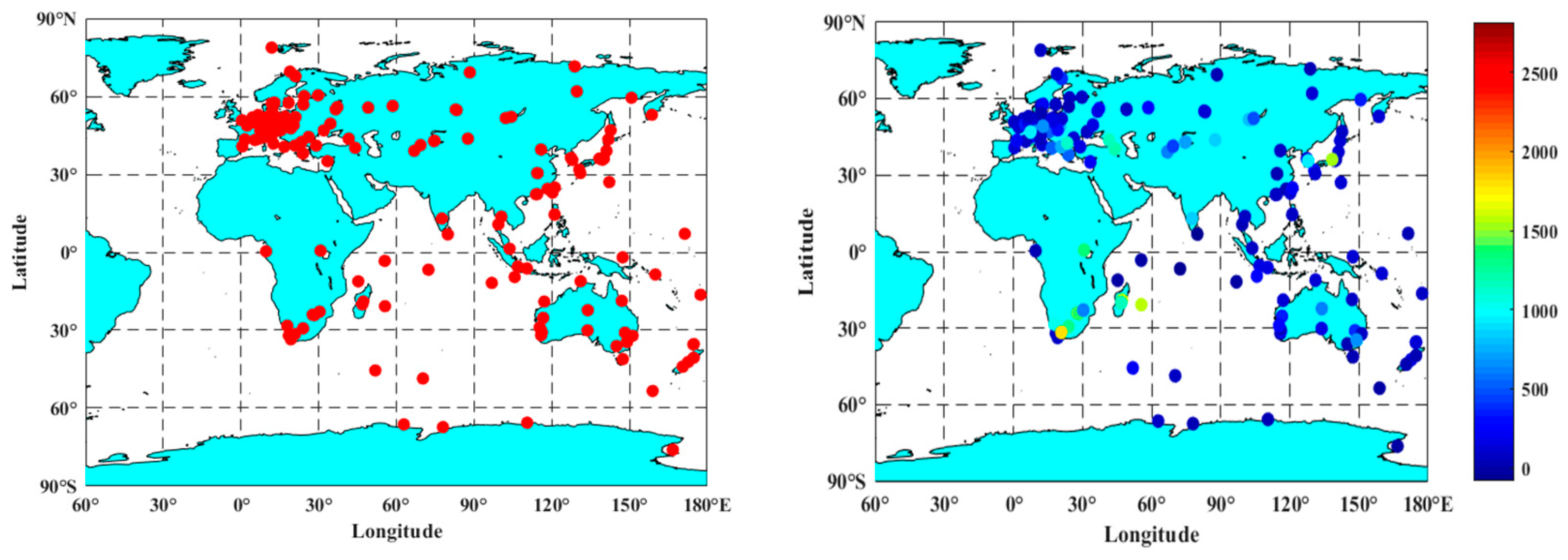
To verify the precision and accuracy of the five tropospheric delay models, the zenith tropospheric delay data provided by CODE in 2019 were used as the reference value, and 297 globally distributed IGS stations were selected for testing. The geographical distribution of the stations is shown in Figure 4. To quantify the accuracy of the five models,

Table 6. Accuracy statistics of the five models compared with ZTD data provided by CODE in 2019 (cm).

Bias/RMS		UNB3m	GPT + Saastamoinen	GPT2w + Saastamoinen	GPT3 + Saastamoinen	GPT3 + Hopfield
Bias	Max	10.6961	10.5927	6.8187	6.8256	6.5690
	Min	−9.6988	−11.5243	−8.3353	−8.3351	−9.5014
	Ave	0.6744	0.2356	−0.4504	−0.4490	−0.1898
RMS	Max	12.5443	11.8738	8.7849	8.7851	9.8982
	Min	1.9381	2.0061	1.5580	1.5584	1.6162
	Ave	4.9968	4.9403	3.9783	3.9759	4.0830

shows the accuracy of the five tropospheric delay correction models.

Table 6 shows that the average Bias and RMS of the UNB3m model were the largest, at 10.6961 cm and 12.5443 cm, respectively. Compared with the UNB3m model, the Bias and RMS values of the four combined models, the accuracy of the GPT + Saastamoinen model was not improved. GPT2w + Saastamoinen, GPT3 + Saastamoinen and GPT3 + Hopfield were smaller; GPT2w + Saastamoinen featured an average Bias of −0.4504 cm, GPT3 + Saastamoinen featured an average Bias of −0.4490 cm and GPT3 + Hopfield averaged −0.1898 cm, and the average of RMS were 3.9783 cm, 3.9759 cm and 4.0830 cm, respectively. Compared with the GPT + Saastamoinen and UNB3m models, the accuracy of the GPT3 + Saastamoinen model was improved by 20.43% and 19.52%, respectively.

In addition, to further analyze the accuracy distribution of the five models, the accuracy statistics of Bias and RMS results were calculated (different colors represent different models). The results are shown in Figure 5 and Figure 6.

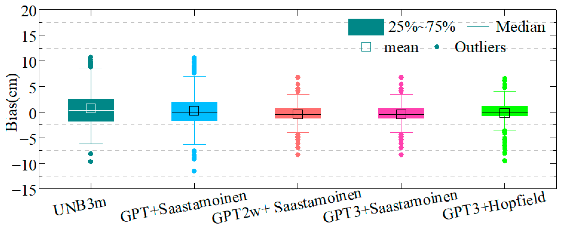
Figure 5 shows that the distribution of the GPT2w + Saastamoinen, GPT3 + Saastamoinen and GPT3 + Hopfield models were more concentrated than the UNB3m model, indicating that the models combined with GPT3 and GPT2w were more stable.

In Figure 6, the RMS is divided into five parts (<3 cm, 3−4 cm, 4−5 cm, 5−6 cm, >6 cm) to analyze the stability of the five models. The RMS of the UNB3m model occupied the largest proportion of 27.95% in the range of greater than 6 cm, but only 9.76% in the range of less than 3 cm. The GPT2w + Saastamoinen, GPT3 + Saastamoinen and GPT3 + Hopfield models accounted for 26.60%, 26.26% and 25.59% of the proportion for less than 3 cm, respectively, and 12.12%, 12.12% and 15.82% for greater than 6 cm. Compared with the UNB3m model and GPT + Saastamoinen model, the accuracy distributions of the other combined models were significantly improved. In the RMS distribution of less than 3 cm, the GPT2w + Saastamoinen, GPT3 + Saastamoinen and GPT3 + Hopfield models increased by 16.84%/16.50%/15.83% and 12.12%/11.78%/11.11%, respectively; in the RMS distribution of greater than 6 cm, they were reduced by 15.83%/15.83%/12.13% and 13.47%/13.47%/9.77%, respectively. Among the five models, GPT3 + Saastamoinen and GPT2w + Saastamoinen had the largest RMS proportional distribution in the range below 4 cm, reaching 67.68%.

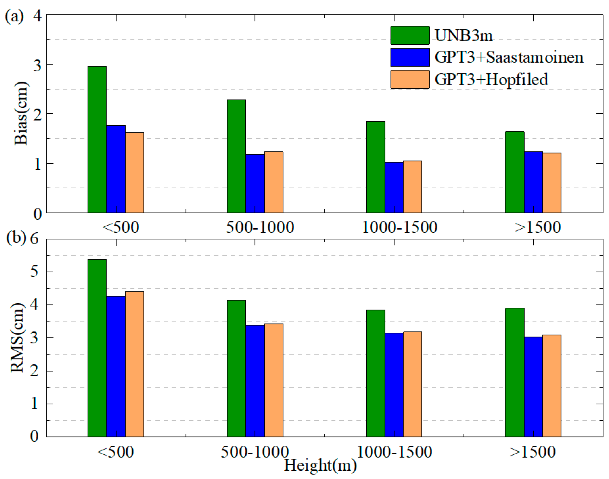
To further analyze the relationship between the Bias and RMS of ZTD estimated by all models according to elevation, the 297 IGS stations were classified at intervals of 500 m, which were divided into five ranges: less than 500 m (213 stations), 500−1000 m (49 stations), 1000−1500 m (18 stations) and greater than 1500 m (17 stations). The Bias and RMS of the three models in each elevation range are shown in Figure 7, and the specific values are counted in

Table 7. Accuracy statistics of three models at different heights verified using ZTD data provided by CODE in 2019 (cm).

Height	UNB3m		GPT3 + Saastamoinen		GPT3 + Hopfield
	Bias	RMS	Bias	RMS	Bias	RMS
<500 m	4.54	5.38	3.46	4.26	3.59	4.40
500–1000 m	3.44	4.15	2.69	3.39	2.76	3.43
1000–1500 m	3.22	3.84	2.54	3.16	2.59	3.18
>1500 m	3.31	3.90	2.90	3.04	2.93	3.09

.

Figure 7 reveals that the GPT3 + Saastamoinen model, the GPT3 + Hopfield model and the UNB3m model showed large absolute Bias values at less than 500 m: 3.46 cm, 3.59 cm and 4.54 cm, respectively; the RMS values were 4.26 cm, 4.40 cm and 5.38 cm, respectively. When the height was greater than 500 m, the Bias values of UNB3m decreased with increasing height, and the Bias of the GPT3 + Saastamoinen model and the GPT3 + Hopfield model were within 3 cm. The RMS values of the GPT3 + Saastamoinen and GPT3 + Hopfield models were less than 5 cm and decreased with increasing height. This is consistent with the phenomenon that ZTD only slightly changes with the increase in height, or the decrease in humidity or temperature [27].

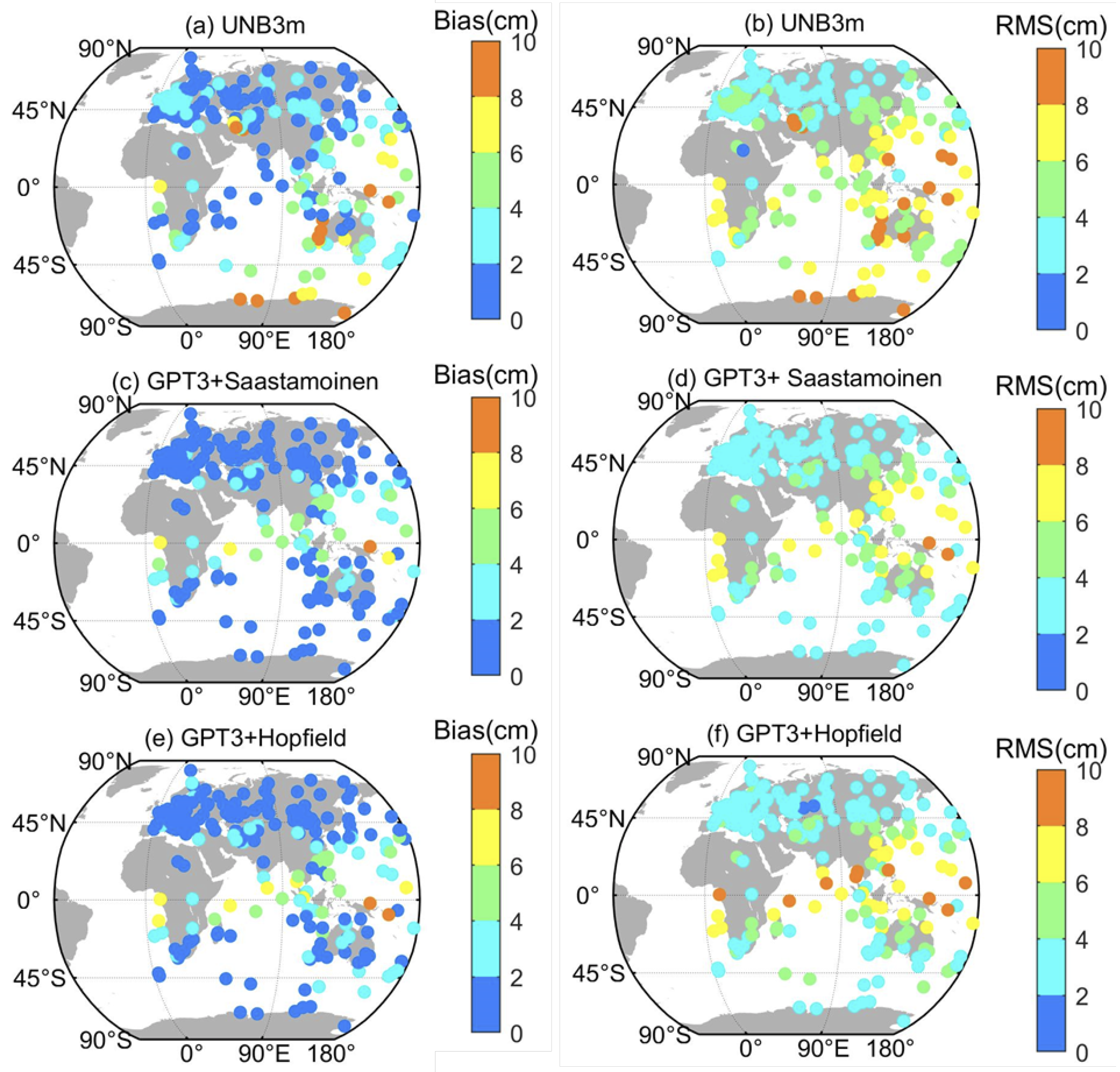
To further study the relationship between the model accuracy and latitude, Figure 8 shows the variation of the deviation and root mean square error of the three models with latitude. The Bias of the UNB3m model in the southern hemisphere was higher than that in the northern hemisphere. Compared with the UNB3m model, the global Biases of the GPT3 + Saastamoinen and GPT3 + Hopfield models were small and stable within 2 cm, but the Bias near the equator was 6−8 cm. The RMS of the UNB3m model in the southern hemisphere and low latitudes was larger, concentrated at 4–10 cm, and the accuracy of the model in the northern hemisphere was significantly higher than that in the southern hemisphere. Globally, the RMS values of the GPT3 + Saastamoinen and GPT3 + Hopfield models were less than 4 cm, except that the RMS near the equator was greater than 6 cm. To better quantify the accuracy of the two models at different latitudes,

Table 8. Bias and RMS values of the three models at different latitudes (cm).

Latitude	UNB3m		GPT3 + Saastamoinen		GPT3 + Hopfield
	Bias	RMS	Bias	RMS	Bias	RMS
Low latitude	0.19	6.30	−1.86	5.45	2.40	5.77
Mid latitude	0.67	4.53	−0.12	3.57	0.36	3.61
High latitude	1.97	4.66	−0.44	2.83	0.57	2.83

shows the Bias and RMS values of the two models at different latitudes.

Table 8 indicates that the three models had great differences in accuracy and applicability at different latitudes. In the middle latitude (30°–60°) and high latitude (60°–90°) regions, the Biases of the GPT3 + Saastamoinen model and the GPT3 + Hopfield model were within 0.60 cm, and the RMS values were within 4 cm; the Bias of the UNB3m model was within 2.00 cm and the RMS value was within 5.00 cm. In low latitudes (0°–30°), the Biases of the GPT3 + Saastamoinen model and the GPT3 + Hopfield model were 1.86 cm and 2.40 cm, respectively, and the RMS values were 5.45 cm and 5.77 cm, respectively. The accuracy and stability of the GPT3 + Saastamoinen model were better than that of the GPT3 + Hopfield model, which was reduced by 22.56% in Bias and 5.67% in RMS. The accuracy of the GPT3 + Saastamoinen model and the GPT3 + Hopfield model was improved by 13.51% and 8.31%, respectively, compared with the UNB3m model.

To explore the seasonal variation characteristics of the three models,

Table 9. Bias and RMS values of the three models in different seasons (cm).

Latitude	UNB3m		GPT3 + Saastamoinen		GPT3 + Hopfield
	Bias	RMS	Bias	RMS	Bias	RMS
January–March	0.97	5.49	−0.36	3.96	−0.05	4.14
April–June	0.50	5.12	−0.58	4.23	−0.32	4.38
July–September	0.24	5.54	−0.62	4.58	−0.46	4.73
October–December	1.12	5.29	−0.14	4.01	0.19	4.14

shows the statistical results of the Bias and RMS values during four seasons (the corresponding months of the four seasons are as follows: January–March, April–June, July–September and October–December). It can be seen from the table that UNB3m revealed the largest Bias with a value of 1.12cm in October–December; the largest Bias of GPT3 + Saastamoinen and GPT3 + Hopfield were −0.62 cm and −0.46 cm in July–September. All three models showed the worst accuracy in July–September; the RMS values were 5.54 cm, 4.58 cm and 4.73 cm, respectively.

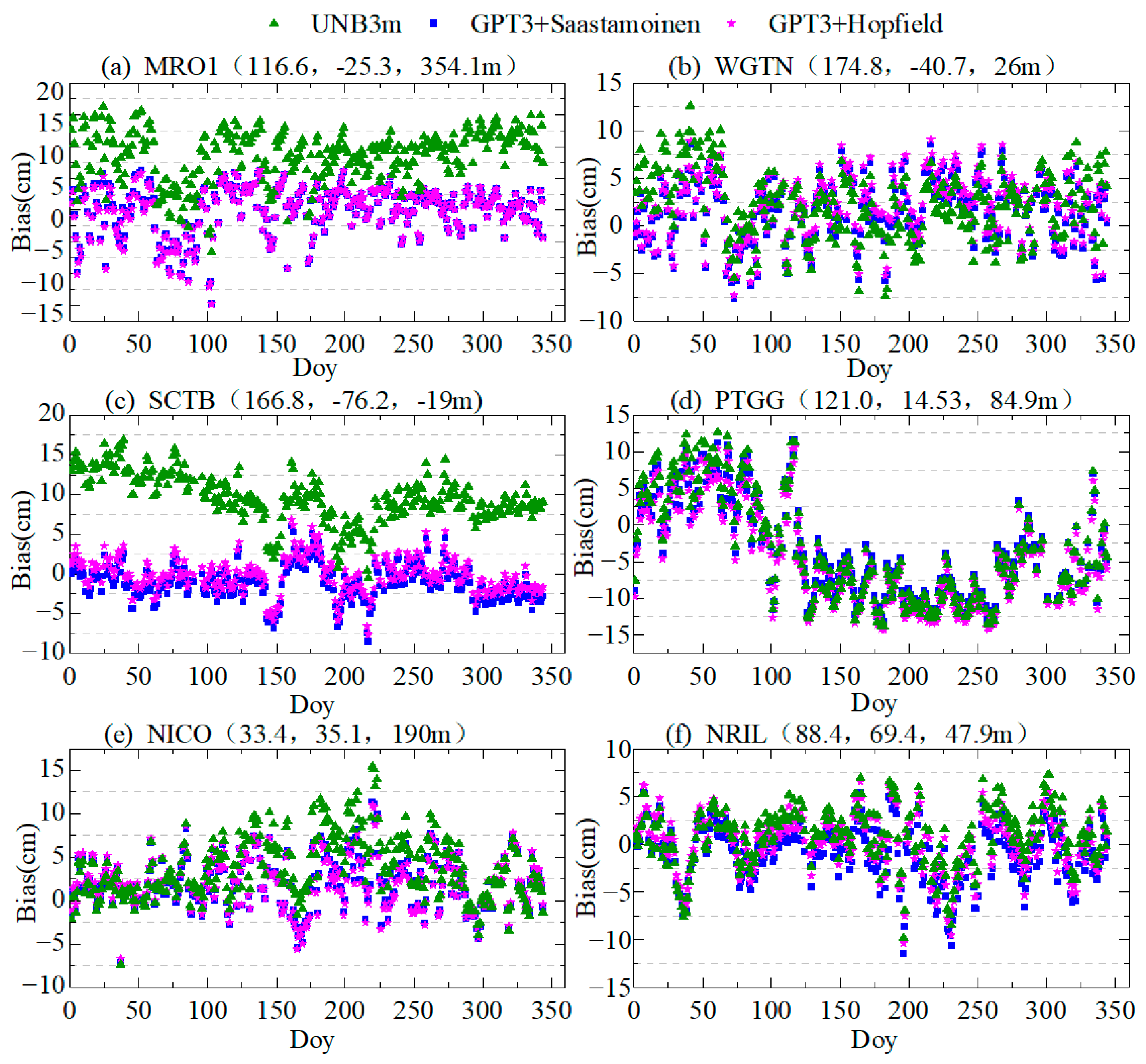
Six IGS stations were selected from the low, middle and high latitudes to further analyze the seasonal variation performance of the three models: MRO1 station (116.6°, 25.3° S, 354.1 m), WGTN station (174.8°, 40.7° S, 26 m), SCTB station (166.8°, 76.2° S, −19 m), PTGG station (121.0°, 14.5° N, 84.9 m), NICO station (33.4°, 35.1° N, 190 m) and NRIL station (88.4°, 69.4° N, 47.9 m) (the brackets indicate the longitude, latitude and height of each station). According to the Bias time series, the accuracy of the three models over different seasons was analyzed.

In Figure 9, for the MRO1 station at a low latitude in the southern hemisphere and the SCTB station at a high latitude in the southern hemisphere, the UNB3m model showed a large positive Bias throughout the year, concentrated at 5–20 cm, especially at low latitudes of the southern hemisphere. In high latitudes in the southern hemisphere, the Biases of the UNB3m model in summer and autumn were higher than that of other seasons, which may be affected by drastic changes in water vapor. The Bias of the GPT3 + Saastamoinen and GPT3 + Hopfield models was relatively stable throughout the year.

For the WGTN station at a middle latitude of the southern hemisphere, the Bias of the UNB3m model was larger in summer compared to the GPT3 + Saastamoinen and GPT3 + Hopfield models; the accuracies of the three models were comparable in the other seasons.

For the PTGG station at a low latitude in the northern hemisphere, the three models had a large positive Bias in winter and a large negative Bias in the other seasons. At the NICO station at the mid-latitude of the northern hemisphere, the absolute Biases of the GPT3 + Saastamoinen and GPT3 + Hopfield models were concentrated between 0 and 5 cm, and the Bias exceeded 5 cm for a few days in summer; the UNB3m model showed a larger Bias between 5 and 15 cm in spring and summer.

For the NRIL station at a high latitude in the northern hemisphere, the absolute Biases of the three models were basically stable within 5 cm, and only a few times in summer and winter. It can be seen that the GPT3 + Saastamoinen and GPT3 + Hopfield models had better accuracy improvements in the southern hemisphere.

4. Discussion

At present, research on the GPT, GPT2 and GPT2w models is very mature, but there are few studies on the accuracy of meteorological parameters estimated by the GPT3 model and its analyses on a global scale. Gao et al. [22] verified and analyzed the GPT3 model in China and found that the deviation of the GPT3 model’s estimation of meteorological parameters was random in low-altitude areas. With the increase in altitude, the Biases for pressure and water vapor pressure gradually stabilized within ±2 hPa, and the temperature stabilized within ±2 °C. In this study, the meteorological parameters in 2018 provided by GGOS Atmosphere were used as experimental reference values. The accuracy of tropospheric product temperature, pressure and water vapor pressure calculated by the GPT3 model and UNB3m, GPT and GPT2w models using globally distributed stations were tested and the seasonal variation characteristics of the GPT3 model were explored. The results showed that the GPT3 model has seasonal characteristics in estimating meteorological parameters, and the temperature Bias was within ±3 °C, the pressure Bias was within ±1.5 hPa and the water vapor pressure Bias value was within ±3 hPa.

Some scholars have combined GPT2/GPT2w with the Saastamoinen model to estimate ZTD in Asia. Liu et al. [27] combined the GPT2 model and the 1° and 5° resolution GPT2w model with the Saastamoinen model, respectively. The Bias value of the GPT2 _ 1w + Saastamoinen model was 0.66 cm and the RMS was 4.93 cm, which were better than those of the GPT2 + Saastamoinen model and the GPT2 _ 5w + Saastamoinen model. However, there are few data on ZTD analyses combined with the GPT3 model. In this study, the GPT3 model was combined with the Saastamoinen model and the Hopfield model to systematically analyze the characteristics of tropospheric delay changes worldwide. The accuracy of the refined tropospheric delay model was verified at different latitudes, heights and in different seasons. The analysis results showed that the GPT3 + Saastamoinen model and the GPT3 + Hopfield model provide tropospheric delay corrections with Biases of −0.33 cm and −0.60 cm and RMS values of 3.98 cm and 4.09 cm, respectively. The Bias values of the two combined models had no obvious relationship with seasonal changes, but were affected by latitude and height. The applicability and accuracy were different at different latitudes and heights.

5. Conclusions

In view of the dependence of the current tropospheric delay correction model on sounding data, this study evaluated the accuracy and spatial–temporal distribution characteristics of the model at different latitudes, elevations and in different seasons. The test results are as follows:

(1)

Using the meteorological parameters provided by GGOS in 2018 as a reference, the accuracies of the UNB3m, GPT, GPT2w and GPT3 models were evaluated. The test results showed that, compared with the UNB3m, GPT and GPT2w models, the accuracy and stability of the GPT3 model were the best, particularly for temperature estimation. The temperature Bias was reduced by 90.60%, 32.44% and 0.30%, respectively, and the temperature RMS was reduced by 42.40%, 11.02% and 0.11%, respectively.

(2)

In different months, the Bias and RMS of the GPT3 model were quite different, indicating that they have obvious seasonality. In terms of temperature, the Bias from October to December was the smallest, with a value of −0.2227 °C. The accuracy was the best from July to September, and its RMS was 3.2926 °C. In terms of atmospheric pressure, the Bias from October to December was the smallest, which was −0.2873 hPa; the highest accuracy was observed from July to September, and the RMS was 4.0990 hPa. In terms of water vapor pressure, the highest accuracy was observed from January to March, with Bias and RMS values of−0.6389 hPa and 2.8166 hPa, respectively.

(3)

At different latitudes, the GPT3 + Saastamoinen model, GPT3 + Hopfield model and UNB3m model had large differences in accuracy and applicability. In the mid-latitude and high-latitude regions, the accuracy of the UNB3m model was lower than that of the GPT3 + Saastamoinen model and the GPT3 + Hopfield model. The Bias of the UNB3m model was within 2.00 cm, and the RMS was within 5.00 cm. The Bias values of the GPT3 + Saastamoinen model and the GPT3 + Hopfield model were less than 0.60 cm, and the RMS values were less than 4.00 cm; at low latitudes, the Bias of the GPT3 + Saastamoinen model was 1.86 cm and the RMS was 5.45 cm. The accuracy and stability of the GPT3 + Saastamoinen model were better than those of the GPT3 + Hopfield model and the UNB3m model, and the accuracy was increased by 5.67 % and 13.5 %, respectively. At different heights, the RMS values of the GPT3 + Saastamoinen model and the GPT3 + Hopfield model were similar and were better than that of the UNB3m model. The accuracy of the three models increased as the height increased when the height was less than 1500 m. At a height of less than 500 m, the three models showed larger Biases (3.46 cm, 3.59 cm and 4.54 cm, respectively). The Biases of the three models were within 3 cm at heights greater than 500 m. In different seasons, the Bias of ZTD estimated by the UNB3m model had obvious seasonal variation throughout the world. The Biases of the GPT3 + Saastamoinen model and the GPT3 + Hopfield model were stable within 5.00 cm. Compared with that of the UNB3m model, the accuracies of the two models in the southern hemisphere were more obvious.

References

1. Zhou, Y.; Lou, Y.; Zhang, W.; Wu, P.; Bai, J.; Zhang, Z. WTM: The Site-Wise Empirical Wuhan University Tropospheric Model. Remote Sens. 2022, 14, 5182. [Google Scholar] [CrossRef]
2. Yao, Y.; Zhao, Q. Research progress and prospect of monitoring tropospheric water vapor by GNSS technique. Acta Geod. Cartogr. Sin. 2022, 51, 935–952. [Google Scholar]
3. Yao, Y.; Zhang, S.; Kong, J. Research Progress and Prospect of GNSS Space Environment Science. Acta Geod. Cartogr. Sin. 2017, 46, 1408–1420. [Google Scholar]
4. Zhao, Q.; Liu, K.; Zhang, T.; He, L.; Shen, Z.; Xiong, S.; Shi, Y.; Chen, L.; Liao, W. A Global Conversion Factor Model for Mapping Zenith Total Delay onto Precipitable Water. Remote Sens. 2022, 14, 1086. [Google Scholar] [CrossRef]
5. Niell, A.E. Global Mapping Functions for the Atmosphere Delay at Radio Wavelengths. J. Geophys. Res. Solid Earth 1996, 101, 3227–3246. [Google Scholar] [CrossRef]
6. Boehm, J.; Niell, A.; Tregoning, P.; Schuh, H. Global Mapping Function (GMF): A New Empirical Mapping Function Based on Numerical Weather Model Data. Geophys. Res. Lett. 2006, 33, 1–4. [Google Scholar] [CrossRef]
7. Kouba, J. Implementation and Testing of the Gridded Vienna Mapping Function 1 (VMF1). J. Geod. 2008, 82, 193–205. [Google Scholar] [CrossRef]
8. Huang, L.; Chen, H.; Liu, L.; Jiang, W. A new high-precision global model for calculating zenith tropospheric delay. Chin. J. Geophys. 2021, 64, 782–795. [Google Scholar]
9. Saastamoinen, J. Contributions to the theory of atmospheric refraction. Bull. Geod. 1972, 105, 279–298. [Google Scholar] [CrossRef]
10. Hopfield, H. Two-quartic Tropospheric Refractivity Profile for Correcting Satellite Data. J. Geophys. Res. 1969, 74, 4487–4499. [Google Scholar] [CrossRef]
11. Black, H.D. An Easily Implemented Algorithm for the Tropospheric Range Correction. J. Geophys. Res. Solid Earth 1978, 83, 1825–1828. [Google Scholar] [CrossRef]
12. Liu, C.; Zheng, N.; Feng, Q. Quality Evaluation of Global Tropospheric Delay Model. J. Geod. Geodyn. 2018, 38, 1005–1010. [Google Scholar]
13. Collins, J.P.; Langley, R.B. The Residual Tropospheric Propagation Delay: How Bad Can It Get? In Proceedings of the 11th International Technical Meeting of the Satellite Division of The Institute of Navigation, Nashville, TN, USA, 15–18 September 1998. [Google Scholar]
14. Penna, N.; Dodson, A.; Chen, W. Assessment of EGNOS tropospheric correction model. J. Navig. 2001, 54, 37–55. [Google Scholar] [CrossRef]
15. Boehm, J.; Heinkelmann, R.; Schuh, H. Short Note: A Global Model of Pressure and Temperature for Geodetic Applications. J. Geod. 2007, 81, 679–683. [Google Scholar] [CrossRef]
16. Leandro, R.F.; Langley, R.B.; Santos, M.C. UNB3m_pack: A neutral atmosphere delay package for radiometric space techniques. GPS Solut. 2008, 12, 65–70. [Google Scholar] [CrossRef]
17. Huang, L.; Liu, L.; Wen, H.; Yao, C. Assessment of zenith tropospheric delay derived from Single-Site Improved EGNOS model over Asia area. Acta Geod. Cartogr. Sin. 2014, 43, 808–817. [Google Scholar]
18. Wang, J.; Chen, J.; Wang, J.; Zhang, J.; Song, L. Assessment of Tropospheric Delay Correction Models over China. Geomat. Inf. Sci. Wuhan Univ. 2016, 41, 1656–1663. [Google Scholar]
19. Zhu, M.; Hu, W.; Wang, L. Accuracy Test and Analysis for GPT2w Model in China. Geomat. Inf. Sci. Wuhan Univ. 2019, 44, 1304–1311. [Google Scholar]
20. Kong, J.; Yao, Y.; Shan, L.; Wang, Z. The Accuracy Analysis of GPT2w at the Antarctic Area. Acta Geod. Cartogr. Sin. 2018, 47, 1316–1325. [Google Scholar]
21. Yang, H.; Feng, K.; Xie, S.; Zhou, Y.; Li, C. An improved GPT2w model based on BP neural network and its global precision analysis. Syst. Eng. Electron. 2019, 41, 500–508. [Google Scholar]
22. Gao, Z.; He, X.; Chang, L. Accuracy analysis of GPT3 Model in China. Geomat. Inf. Sci. Wuhan Univ. 2021, 46, 538–545. [Google Scholar]
23. Li, S.; Xu, T.; Xu, Y.; Jiang, N.; Luísa, B. Forecasting GNSS Zenith Troposphere Delay by Improving GPT3 Model with Machine Learning in Antarctica. Atmosphere 2022, 13, 78. [Google Scholar] [CrossRef]
24. Li, Q.; Yuan, L.; Chen, P.; Jiang, Z. Global Grid-Based Tm Model with Vertical Adjustment for GNSS Precipitable Water Retrieval. GPS Solut. 2020, 24, 73. [Google Scholar] [CrossRef]
25. Huang, L.; Zhu, G.; Peng, H.; Liu, L.; Ren, C.; Jiang, W. An Improved Global Grid Model for Calibrating Zenith Tropospheric Delay for GNSS Applications. GPS Solut. 2023, 27, 17. [Google Scholar] [CrossRef]
26. Zhu, G.; Huang, L.; Yang, Y.; Li, J.; Zhou, L.; Liu, L. Refining the ERA5-Based Global Model for Vertical Adjustment of Zenith Tropospheric Delay. Satell. Navig. 2022, 3, 27. [Google Scholar] [CrossRef]
27. Liu, J.; Chen, X.; Sun, J.; Liu, Q. An analysis of GPT2/GPT2w+Saastamoinen models for estimating zenith tropospheric delay over Asian area. Adv. Space Res. 2017, 59, 824–832. [Google Scholar] [CrossRef]
28. Yang, Y.; Yu, G.; Pan, S.; Chen, W.; Wang, D. A comprehensive algorithm using fusion of tropospheric delay models. J. Southeast Univ. 2013, 43, 418–422. [Google Scholar]
29. Yao, Y.; Zhang, B.; Yan, F.; Xu, C.Q. Two new sophististicated models for tropospheric delay corrections. Chin. J. Geophys. 2015, 58, 1492–1501. [Google Scholar]
30. Yang, H.; Hu, W.; Yu, L.; Nie, X.; Li, H. GHop: A New Regional Tropospheric Zenith Delay Model. Geomat. Inf. Sci. Wuhan Univ. 2020, 45, 226–232. [Google Scholar]
31. Du, X.; Qiao, J.; Wei, P. Real-time Correction Model for Zenith Tropospheric Delay Applied to the Chinese Region. J. Electron. Inf. Technol. 2019, 41, 156–164. [Google Scholar]
32. Liu, Z.; Chen, X.; Liu, Q.; Zhang, S. Estimation Zenith Tropospheric Delay Based on Multi-Source Data. J. Astronaut. 2020, 41, 586–591. [Google Scholar]
33. Yang, F.; Guo, J.; Meng, X.; Li, J.; Zhou, L. A global grid model for calibration of zenith hydrostatic delay. Adv. Space Res. 2021, 68, 3574–3583. [Google Scholar] [CrossRef]
34. Xu, T.; Li, S.; Wang, S.; Nan, J. Improved tropospheric delay model for China using RBF neural network and meteorological data. Acta Geod. Cartogr. Sin. 2022, 51, 1690–1707. [Google Scholar]
35. Lagler, K.; Schindelegger, M.; Böhm, J.; Krásná, H.; Nilsson, T. GPT2: Empirical Slant Delay Model for Radio Space Geodetic Techniques. Geophys. Res. Lett. 2013, 40, 1069–1073. [Google Scholar] [CrossRef]
36. Böhm, J.; Möller, G.; Schindelegger, M.; Pain, G.; Weber, R. Development of an Improved Empirical Model for Slant Delays in the Troposphere (GPT2w). GPS Solut. 2015, 19, 433–441. [Google Scholar] [CrossRef]
37. Landskron, D.; Böhm, J. VMF3/GPT3: Refined discrete and empirical troposphere mapping functions. J. Geod. 2018, 92, 349–360. [Google Scholar] [CrossRef]
38. Dow, J.M.; Neilan, R.E.; Rizos, C. The International GNSS Service in a Changing Landscape of Global Navigation Satellite Systems. J. Geod. 2009, 83, 689. [Google Scholar] [CrossRef]
39. Ding, J.; Chen, J.; Wang, J. Quality Control Method for ZTD Modeling Based on GNSS Observation Data. J. Astronaut. 2020, 41, 1195–1203. [Google Scholar]
Figure 1. Geographical distribution of the 25 IGS stations.
Atmosphere 14 00946 g001
Figure 2. Temperature (a), atmosphere pressure (b) and water vapor pressure (c) estimated by four non-measured meteorological parameter models compared with GGOS Atmosphere.
Atmosphere 14 00946 g002
Figure 3. Bias (a,c,e) and RMS (b,d,f) of four non-measured meteorological parameter models estimated using 25 IGS stations.
Atmosphere 14 00946 g003
Figure 4. The geographical distribution of the 297 selected IGS stations. (Left: station distribution map; Right: station elevation map).
Atmosphere 14 00946 g004
Figure 5. Bias of five models validated using ZTD data provided by CODE in 2019.
Atmosphere 14 00946 g005
Figure 6. RMS proportional distribution of the five models validated using ZTD data provided by CODE in 2019.
Atmosphere 14 00946 g006
Figure 7. Changes in Bias (a) and RMS (b) values of three models at different heights verified using ZTD data provided by CODE in 2019 (cm).
Atmosphere 14 00946 g007
Figure 8. Global distribution of Bias (ac) and RMS (df) values of the three models.
Atmosphere 14 00946 g008
Figure 9. Bias time series of the three models using six IGS stations (the brackets indicate the longitude, latitude and height of each station) verified using ZTD data provided by CODE in 2019. ((af) represent the Bias of MRO1, WGTN, SCTB, PTGG, NICO, NRIL station).
Atmosphere 14 00946 g009