Article

Underrepresentation of the Linkage between the Barents–Kara Sea Ice and East Asian Rainfall in Early Summer by CMIP6 Models

Key Laboratory of Meteorological Disaster of Ministry of Education/ICAR/Collaborative Innovation Center on Forecast and Evaluation of Meteorological Disasters, Nanjing University of Information Science and Technology, Nanjing 210044, China
*
Author to whom correspondence should be addressed.
Atmosphere 2023, 14(6), 1044; https://doi.org/10.3390/atmos14061044
Submission received: 16 May 2023 / Revised: 11 June 2023 / Accepted: 13 June 2023 / Published: 17 June 2023
(This article belongs to the Topic Cryosphere: Changes, Impacts and Adaptation)

Abstract

:
Our previous study revealed the link between Barents–Kara sea ice and rainfall in eastern China. This study continues evaluating the performance of multiple models from phase 6 of the Coupled Model Intercomparison Project (CMIP6) in simulating this linkage. Most CMIP6 models can simulate Arctic sea ice coverage in the present climate system, although the sea ice extent in the edge areas show some biases. Only a few models can roughly reproduce the observed rainfall dipole pattern associated with Arctic sea ice variability. The linkage between Arctic sea ice variability in winter and eastern China rainfall in early summer is performed through a long memory of the sea ice, the stratospheric variability as the mediator, and downward propagation of stratospheric signals. Very few CMIP6 models can exhibit a realistic interannual relationship between the Arctic sea ice and China rainfall. The selected high-skill models with a more realistic linkage between sea ice and China rainfall present a clear downward impact of the stratospheric circulation anomalies associated with sea ice variability. The reversal of the Northern Hemisphere Annular Mode (NAM) from the negative phase in early winter to the positive phase in spring in the high-skill models and observations denotes the important role of the stratosphere as a mediator to bridge the Arctic sea ice and China rainfall. The long memory of the Arctic sea ice with the stratosphere as the mediator has a deep implication on the seasonal forecasts of East Asian countries.

1. Introduction

In recent decades, significant changes have taken place in the Arctic climate system. It is widely reported that the Arctic has exhibited dramatic warming in the last decades, known as Arctic amplification [1,2]. As an important part of the climate system, Arctic sea ice can change the atmospheric circulation and it plays an important role in the atmospheric variation in middle and high latitudes [3]. Arctic sea ice has a significant impact on the Eurasian climate [4,5,6]. The loss of Arctic sea ice can enhance the sea–air heat flux exchange and affect climate through positive sea ice feedback [7], atmospheric temperature feedback [8], and cloud and water vapor feedback [9]. However, there are still some debates on the extent to which changes in sea ice affect mid and high latitude atmospheric circulation and climate [10]. Some studies have suggested that the Arctic warming likely increases blocking circulation anomalies in some regions of the Northern Hemisphere, leading to more extreme weather events [11], although the blocking circulation does not show much of a long-term trend in other regions [12]. A recent study reported that sea ice loss over Barents–Kara Seas can excite significant positive geopotential height anomalies over the Arctic region and negative anomalies over Eurasia, which resembles a wave train [13].
The global climate is significantly affected by changes in Arctic sea ice, and some studies emphasize the lead/lag relationship between the Barents–Kara sea ice forcing and regional climate. For example, sea ice forcing in late autumn is closely related to the North Atlantic Oscillation (NAO) in winter; therefore, Barents–Kara sea ice is a suitable predictor for NAO. Eurasia is vulnerable to a cold winter after an unusual loss of Arctic sea ice in autumn [14,15]. Conversely, an increase of Arctic sea ice in autumn usually corresponds to a weakening of the Siberian high and an increase in East Asian temperature in winter [16]. Furthermore, Arctic sea ice forcing can trigger wave trains over the Northern Hemisphere and cause sea surface temperature anomalies in the North Pacific Ocean, which in turn affect East Asian summer circulation [17]. The autumn and winter sea ice have also been shown to have a persistent lag effect [16,18].
Previous studies [17,19] have indicated that Arctic sea ice is a major factor affecting summer precipitation over eastern China. The circulation pattern and precipitation over North China in summer are significantly influenced by the Arctic sea ice in the preceding winter [19]. Yang et al. [20] indicated that the Arctic sea ice in the Barents–Kara Seas likely has a delayed effect on summer precipitation across eastern China. On the longer timescale, a significant negative correlation between spring Arctic sea ice and summer precipitation in South China has been revealed, corresponding to the Eurasia–South China decadal teleconnection pattern [21,22,23]. By altering atmospheric circulation, persistent signals of sea ice variabilities finally lead to changes in East Asian summer precipitation [17,24].
Some previous studies mainly focused on the tropospheric circulation changes associated with Arctic sea ice [11,25], while other studies also emphasized the stratospheric role [26,27], although the response of the stratosphere to the sea ice anomaly is overall weaker than that of the troposphere [28]. Sun et al. [29] indicated that the impact of sea ice anomalies on weather and climate in Eurasia was significantly modulated by stratospheric circulation. The impact of sea ice forcing on tropospheric circulation is featured with significant changes in the blocking highs [30,31] or the Siberian high intensity, and therefore results in Eurasian climate anomalies [32,33]. In contrast, the stratospheric pathway for the Arctic sea ice forcing is focused on the polar vortex [20,26,34]. For example, the anomalous sea ice loss in the Barents–Kara Seas in early winter can lead to wider open water and more turbulent heat exchange between the atmosphere and surface, which excites Rossby planetary waves propagating upward into the stratosphere. As a result, the active wave activities in the stratosphere weaken the intensity of the stratospheric polar vortex, which is usually projected onto the negative phase of the Arctic Oscillation, and cold extremes follow in Eurasia [26,34,35]. Yang et al. [20] further identified the medium role of the stratospheric variability in linking the Arctic sea ice forcing in winter and China climate anomalies in early summer.
Simulations of Arctic sea ice have been assessed for several generations in Coupled Model Intercomparison Projects (CMIPs), and the performance of models has gradually improved [36,37,38]. Some studies showed that Chinese CMIP6 models reasonably simulate the spatial pattern of long-term mean sea ice drift in polar regions. Existing evidence indicates that coupled models still have large uncertainties in reproducing the sea ice amplitude and long-term trends [39]. However, we still do not know to what extent the relationship between Arctic sea ice and China’s rainfall is simulated by CMIP models. Using the state-of-the-art coupled models from CMIP6, this relationship can be assessed. Furthermore, the physical processes responsible for this relationship are compared among models, with an expectation to better understand China’s climate changes associated with the polar forcing.
The paper is organized as follows. Following the introduction in Section 1, Section 2 describes the CMIP6 models, datasets, and methods employed in this study. The overall simulation of climatology and variability of Arctic sea ice cover in CMIP6 is assessed in Section 3 for individual models and using the multi-model ensemble mean (MME). The Section 3 also compared linkage between Arctic sea ice and eastern China rainfall and explored the dynamical diagnosis for the circulation changes associated with Barents–Kara sea ice forcing for CMIP6 models. Finally, Section 4 and Section 5 present a discussion and summary, respectively.

2. Materials and Methods

2.1. Data

To evaluate the performance of the Arctic sea ice−precipitation relationship in CMIP6 models, monthly sea ice concentration (SIC) data from the Hadley Centre Sea Ice and Sea Surface Temperature dataset (HadISST) provided by the Met Office Hadley Centre are used [40], which has a 1° × 1° (latitude × longitude) horizontal resolution and ranges from 1870 to the near present. SIC is given as a percentage of the grid box area covered with ice. The fifth-generation reanalysis of ECMWF (ERA5) [41] is used to diagnose atmospheric circulation anomalies associated with SIC changes. ERA5 has an equivalent native grid of 0.25° × 0.25° (latitude × longitude) and 37 pressure levels. We obtained this dataset at a resolution of 1° × 1° for easy handling of data. Different variables are used in this study, including the geopotential (divided by 9.8 to obtain the geopotential height), zonal wind, and meridional wind. The precipitation observations are provided by the Climate Prediction Center Merged Analysis of Precipitation (CMAP), which spans from 1979 to the near present [42]. Global Precipitation Climatology Centre monthly precipitation (GPCC) is also used to confirm the statistical results [43].
The Barents–Kara sea ice index refers to the area-averaged mean of sea ice concentration in the region enclosed by 65–85° N, 20–90° E. This study aims to expand the analysis of Yang et al. [20], including eastern China, which has been shown to be significantly correlated with sea ice in the Barents–Kara Seas. The region is roughly to the north and the other to the south of the Yangtze River. The rainfall in the two regions is averaged to denote the rainfall indices.

2.2. CMIP6 Models and Outputs

The World Climate Research Program (WCRP) has launched a series of CMIPs (i.e., CMIP3, CMIP5, andCMIP6), and the scientific results from them provide abundant materials for the assessment reports for the United Nations Intergovernmental Panel on Climate Change (IPCC) (e.g., AR4, AR5, and AR6) in response to the increasingly uncertain global climate challenge [44,45,46]. Forty-eight CMIP6 models were selected to assess the sea-ice−China rainfall linkage. Details of the models are shown in Table 1, including their atmospheric horizontal resolutions, vertical levels, the model-lid height, and the sea ice model component. Many existing models were updated to a newer version for CMIP6 compared with the previous CMIPs (e.g., CMIP3 and CMIP5). However, the design of historical experiments in CMIP6 was almost identical to that in CMIP5, subject to all the forcings in the 20th century (e.g., greenhouse gas concentrations, aerosols, ozone depletion, solar cycles, and anthropogenic land use) [46]; adjustments were made for the forcing of volcanic eruptions and concentrations of key greenhouse gases such as carbon dioxide. The start year of historical runs for CMIP6 was 1850 and the end year was 2014. We used the bilinear interpolation scheme to reconstruct all CMIP6 data on an equivalent 1° × 1° (latitude × longitude) grid resolution, although the models had different nominal resolutions.
High-top models refer to ones with a model top above 1 hPa (~50 km) and low-top models refer to ones with a model top below 1 hPa [47,48]. The high-skill models refer to ones that simulate the rainfall dipole centers in eastern China associated with SIC variability [20], and low-skill models refer to ones that miss the rainfall dipole centers.

3. Results

3.1. Climatology and Variability of Barents–Kara Sea Ice in CMIP6 Models

The climatology and variability of the Arctic sea ice concentration averaged for November and December from 1979–2020 (1973–2014) are shown in Figure 1 for the Hadley Center observations, high-skill models, and low-skill models. Previous studies have suggested that the sea ice concentration (SIC) variability is maximized in November and December [49]. Therefore, we focused on early winter SIC. According to observations (Figure 1a,b), most of the Arctic Ocean is fully covered with sea ice, except for a few Arctic boundary areas and some Arctic islands (Figure 1a). It has been shown that most parts of the North Pacific and North Atlantic Oceans are nearly free from sea ice. Regions with full sea ice coverage and open waters have an insignificant interannual variability of SIC (Figure 1b). The largest SIC variability is located in high-latitude regions such as Barents–Kara Seas, the Bering Strait, and the Greenland Sea. All of these regions with significant SIC variability are not fully covered with sea ice and are in the transition band neighbored by large-scale sea ice poleward and open waters equatorward. In contrast, the Barents–Kara Seas are covered by the highest SIC variability, which is marked by a purple sector box in Figure 1 (65–85° N, 20–90° E). It has been controversial whether the SIC forcing in Barents–Kara Seas can affect the climate in Eurasia [14,50]. However, as a typical area with strong air−sea interactions, the Barents–Kara Seas are still a key region in the Arctic with the largest SIC variability in early winter [51,52,53].
CMIP6 models diverge in the simulation of Arctic SIC climatology and variability. CMIP6 models with a relatively high skill of simulating SIC and the Arctic sea ice−China rainfall relationship (BCC-ESM1, CAMS-CSM1-0, E3SM-1-1-ECA, and EC-Earth3-Veg; # 5, 6, 20, and 23) and those with a relatively low skill (CAS-ESM2-0, FGOALS-g3, GISS-E2-1-G, and GISS-E2-1-G-CC; # 9, 25, 30, and 31) are shown in Figure 1c–f, respectively. Compared with the observations, the MME of high-skill models shows a wider sea ice cover in the entire Arctic nearly (Figure 1c). However, the MME of low-skill models simulate a much wider sea ice cover than high-skill models, especially in Barents−Kara Seas (Figure 1e). For the sea ice variability in early winter, the MME for high-skill models is fairly consistent with observations, although the SIC variability in Barents–Kara Seas is underestimated (Figure 1d). In contrast, the SIC variability in the low-skill models is much smaller than in the observations and high-skill models (Figure 1f). Overall, the SIC variability in Barents–Kara Seas is smaller in low-skill models than in high-skill models and observations in most Arctic regions, but those in Greenland Sea and Norway Sea are overestimated obviously, which is largely biased from observations.
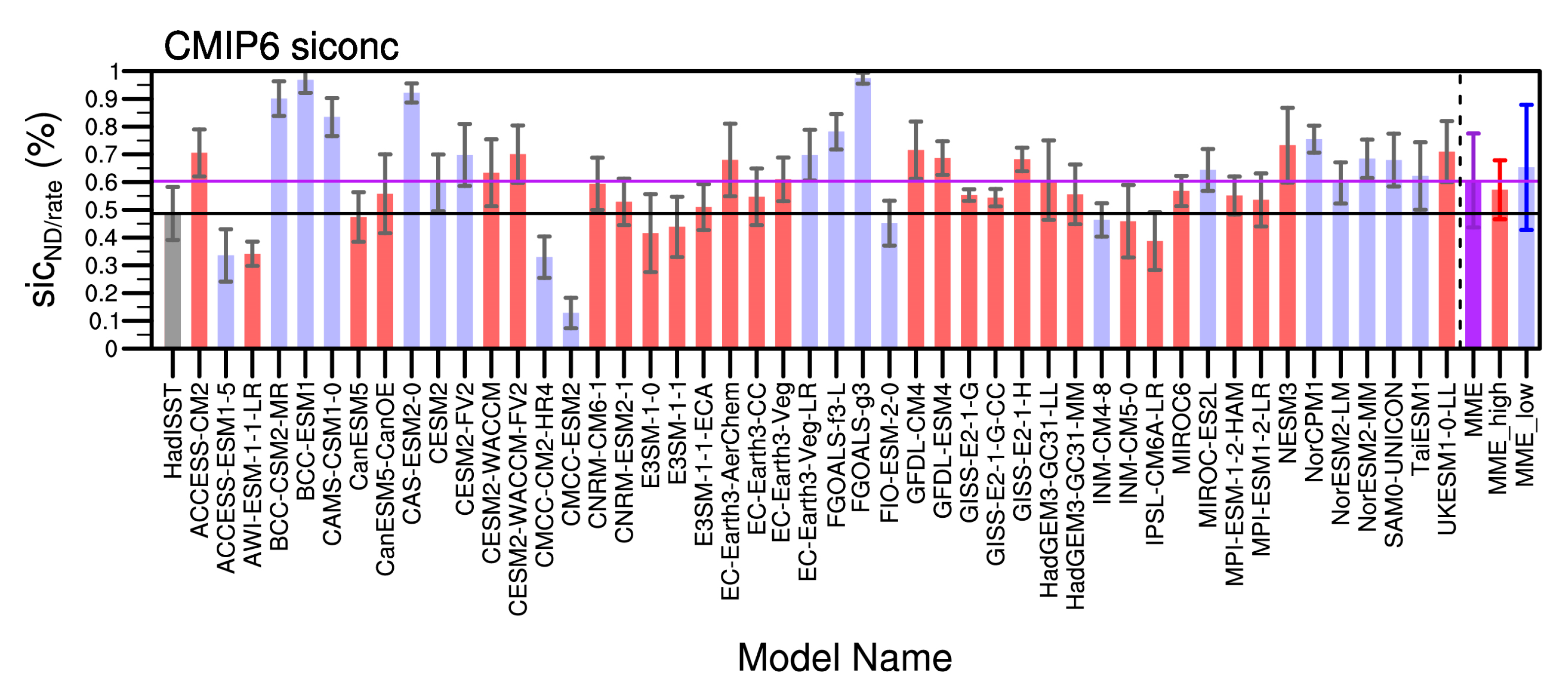
To provide an overall insight into the CMIP6 simulation of Barents–Kara sea ice, a parallel comparison of the SIC climatology and variability in Barents–Kara Seas is shown in Figure 2. The bimonthly SIC mean in Barents–Kara Seas in observations is about 49% with a SIC variability of 9%. The SIC climatology in the CMIP6 MME is overestimated, but close to the observations. Several models reproduce a mean state nearly identical to observations, and typical ones are CanESM5 and E3SM-1-1-ECA. Furthermore, some CMIP6 models overestimate the SIC variability in Barents–Kara Seas. The mean SIC in 14 CMIP6 models (ACCESS-CM2, BCC-CSM2-MR, BCC-ESM1, CAMS-CSM1-0, CAS-ESM2-0, CESM2-FV2, CESM2-WACCM-FV2, EC-Earth-Veg-LR, FGOALS-f3-L, FGOALS-g3, GFDL-CM4, NESM3, NorCPM1, and UKESM1-0-LL) is significantly larger than that in observations (>70%), while the mean SIC in 5 CMIP6 models (ACCESS-ESM1-5, AWI-ESM-1-1-LR, CMCC-CM2-HR4, CMCC-ESM2, and IPSL-CM6A-LR) is significantly underestimated (<40%). In addition, the mean SIC in 15 models is overestimated but falls into the values ranging between the observations and the MME of all CMIP6 models, while those in the remaining 6 models are little less than in the observations. The MME for all models of mean SIC is nearly 60% higher than the observations. Further analysis shows that the MME of climatic state and variability is better simulated by high-top models than low-top models (58% vs. 63%; 8% vs. 20%), although no evidence indicates that the stratospheric process is a deterministic factor for Arctic sea ice simulation at present. In summary, SIC biases are still present in CMIP6 models, most of which are overestimated. The existing SIC biases in most models at the present stage pose large uncertainties on the accurate projection of future climate change.

3.2. Impact of the Barents–Kara Sea Ice on June Rainfall in Eastern China in CMIP6

3.2.1. Divergent Rainfall Patterns Associated with Arctic Sea Ice Change

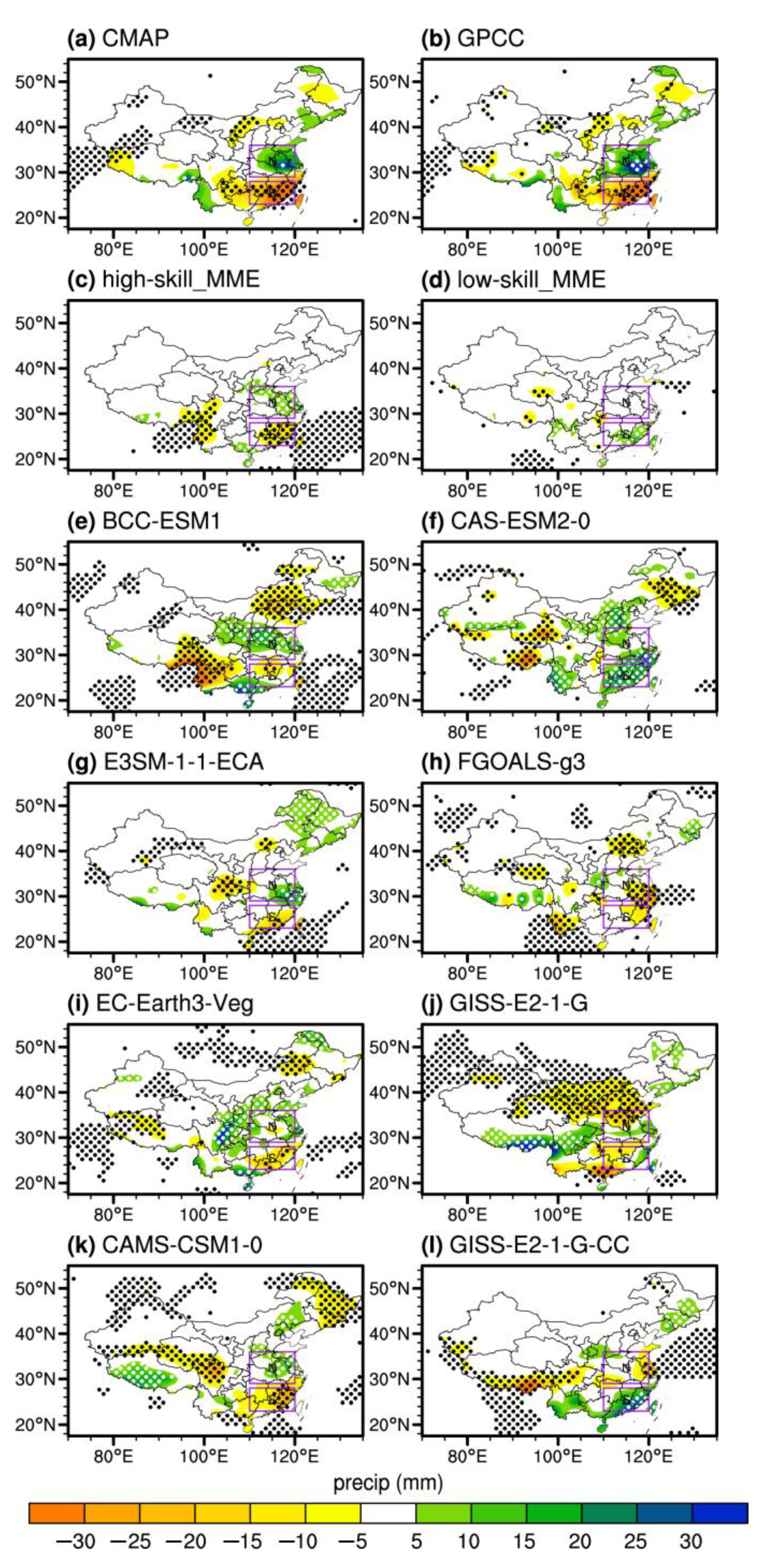
SIC in Barents–Kara Seas has the largest variability across the Arctic Ocean, and it has decreased in past decades with global warming [20,54]. Barents–Kara Seas is a key region and SIC variability has thus been shown to have some implications for seasonal forecasts in parts of East Asia [17,53,55]. The regressed rainfall anomalies in June (units: mm) against the standardized SIC in Barents–Kara Seas from observations and several representative CMIP6 models are shown are Figure 3. Models with a better reproducibility of the rainfall response and those with a worse reproducibility are shown, respectively. According to the observations and results from our previous study [20], the increase (decrease) in Barents–Kara sea ice in the preceding early winter usually leads to anomalously less (more) precipitation in South China and anomalously more (less) precipitation to the north of Yangtze River (Figure 3a,b).
High-skill models and their MME can reproduce the precipitation anomaly pattern in eastern China, which resembles the observed rainfall dipole (Figure 3c,e,g,i,k). Typical high-skill (BCC-ESM1, E3SM-1-1-ECA, EC-Earth3-Veg, and CAMS-CSM1-0) models and their MME are better matched with the observations than the other models. In contrast, some models fail to reproduce the rainfall dipole, but simulate a monopole pattern, a shifted pattern, or even a reversed pattern. Typical low-skill models (CAS-ESM2-0, FGOALS-g3, GISS-E2-1-G, and GISS-E2-1-G-CC) and their MME generally simulate an overall opposite pattern to the observations or an illusory monopole pattern (Figure 3d,f,h,j,l). Overall, high-skill models’ MME resembles a matched rainfall dipole and shows a much better predictive capability, although the rainfall anomalies are underestimated. In addition, we conducted a significance test/robustness examination on the results in Figure 3 and the black/white dots mark regression at the 95% confidence level in the coupled model simulation.
Reasons for underrepresentation of the Arctic sea ice−China climate linkage by CMIP6 models are complicated, and biases in the simulated sea ice and rainfall, as well as complexity of the response of atmospheric circulation to sea ice [30,32], can lead to the loss of this link. Furthermore, responses of weather and climate in mid-to-high latitudes to sea ice forcing in different regions are also not identical [29,56], so biases in the SIC variability across the Arctic can also distort the observed relationship between Barents–Kara sea ice and China rainfall.

3.2.2. Multi-Model Comparison

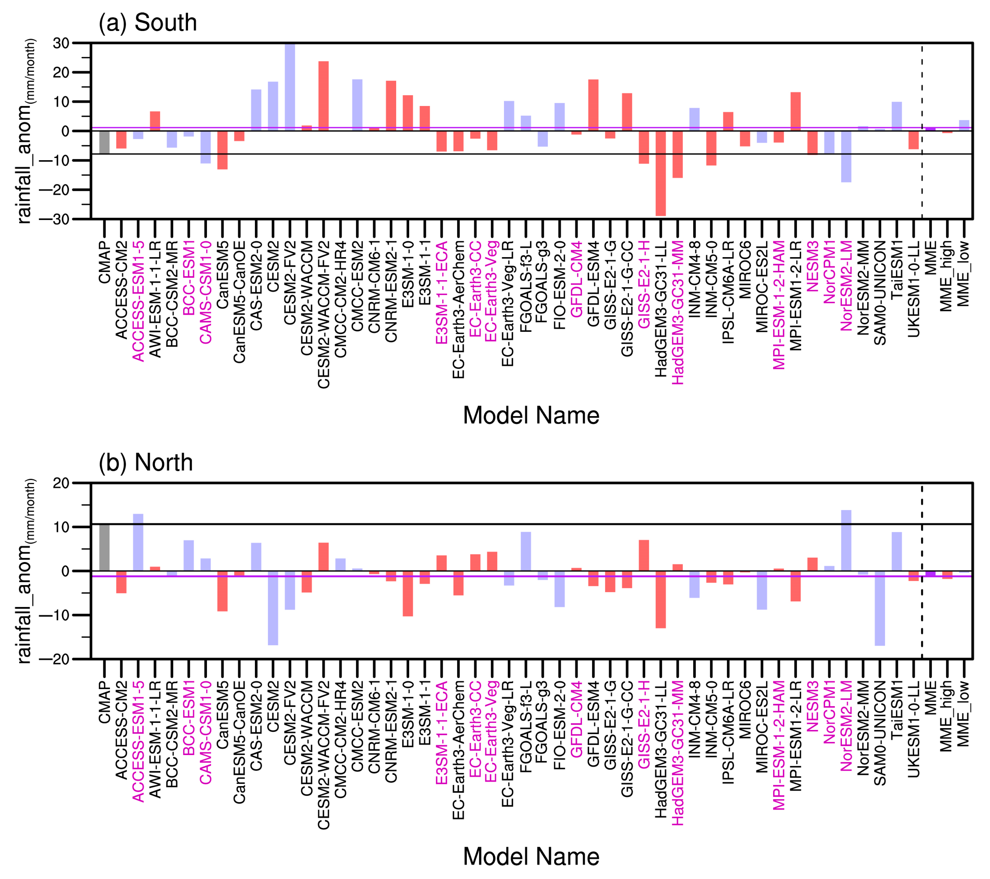
Figure 4 shows the regressed rainfall anomalies in two focused regions against the standardized SIC in Barents–Kara Seas for the observations and 48 CMIP6 models. In the observations, most regions of South China are covered by negative rainfall anomalies when the Barents–Kara sea ice increases (Figure 4a). Four high-top models (CanESM5, CESM2-WACCM, GISS-E2-1-H, and INM-CM5-0) can simulate the drier signal, which is similar to the observations (−7.5 mm). Twenty-two models fail to simulate the drier signal with the sign reversed (illusive wetter signal). Three models (HadGEM3-GC31-LL, HadGEM3-GC31-MM, and NorESM2-LM) simulate the negative rainfall anomalies with the amplitude largely overestimated (−20 mm). The MMEs of regression for all, high-top, and low-top models are shown, respectively. MMEs also show little skills in simulating the Arctic sea ice–China rainfall linkage. For the second focused region in the north, more rainfall is observed when the Barents SIC increases (Figure 4b). As two representatives of high-skill models in the reproduction of this link between Barents–Kara Sea SIC and eastern China rainfall, NorESM2-LM and FGOALS-f3-L can well reproduce the positive correlation between Barents–Kara sea ice and June precipitation, nearly identical to the observations (11 mm). There are 21 models simulating the positive rainfall anomalies, but the amplitude of the anomalies is underestimated in these models. One model (TaiESM1) simulates the positive rainfall anomalies with the amplitude largely overestimated (15 mm). The remaining models are not even skilled at capturing the signs of regressed rainfall anomalies.
The MMEs for different groups (high-top, low-top, and all models) also show little skill, which denotes that most CMIP6 models still lack a reasonable reproducibility of the Arctic SIC–China climate relationship. However, there are still 13 models (marked ID in Figure 4) that show matched rainfall anomalies dipole mode. Overall, the reproducibility of the Arctic SIC–China climate relationship still needs to be improved in the future.

3.3. Physical Processes Associated with Barents–Kara Sea Ice Forcing

3.3.1. Long Memory of Arctic Sea Ice

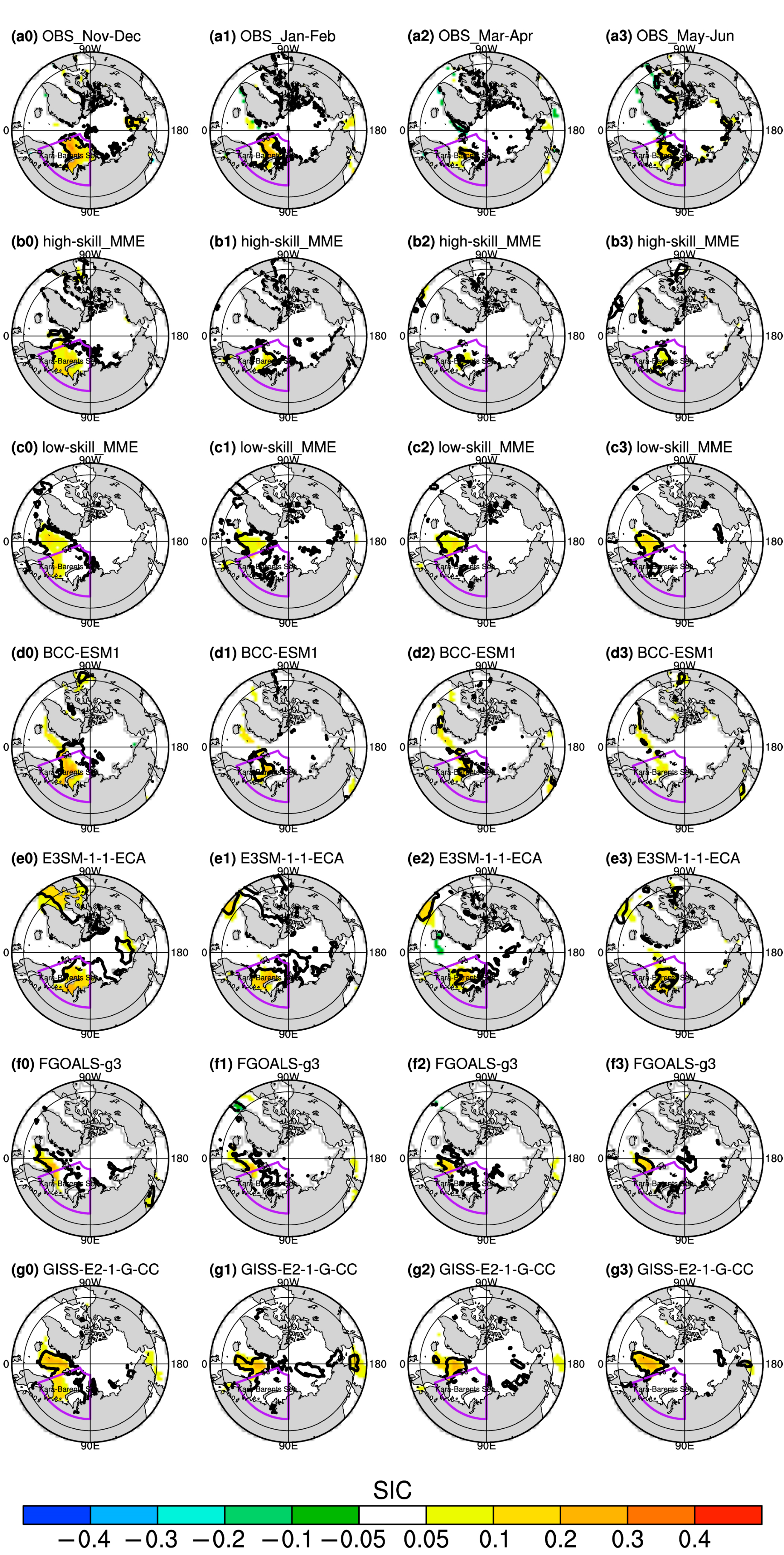
The possible impact of spring–summer Arctic sea ice anomalies on the Northern Hemisphere atmospheric circulation has been investigated in recent studies [9,57]. The mid-latitude summer circulation in the Northern Hemisphere is significantly modulated by Arctic SIC forcings, and the vortex intensity and westerlies weaken during sea ice loss [58]. Furthermore, SIC usually has a long memory, and the sea ice anomaly forcing from November to June enhances the persistent lagged effects on circulation and regional climate [20,59,60]. Figure 5 shows the lead/lag regression of sea ice anomalies against the Barents–Kara sea ice index for the observations and models. Following significant sea ice change in Barents–Kara Seas (65–85° N, 20–90° E) in November and December, this anomalous signal remains until January and February. In March and April, it is still clearly present, although the extent shrinks. Afterwards, this abnormal response of sea ice cover in the Barents−Kara Sea persists until May and June with a second intensification (Figure 5a–d).
The MME for selected high-skill CMIP6 modes and typical high-skill models (BCC-ESM1 and E3SM-1-1-ECA) realistically simulates the long memory of the Arctic SIC in Barents–Kara Seas (Figure 5b0–b3, d0–d3, and e0–e3). The SIC anomalies are largest in November and December, and gradually weaken in the following months. The general SIC anomaly pattern is still present even until May–June, highly resembling observations. In contrast, low-skill models and their MME fail to simulate a long memory for SIC effectively, and the Arctic SIC anomaly pattern is soon torn into pieces in January–February and shrinks heavily in the following months. Models fail to simulate the second enhancement of SIC anomalies in May−June (Figure 5c0–c3, f0–f3, and g0–g3). Furthermore, the SIC anomaly magnitude for the high-skill models is also more realistic than for low-skill models. The relatively weak self-persistence of the SIC anomalies in low-skill models might explain the missing relation between China’s climate and Barents–Kara sea ice variability. In addition, the impact of rainfall over East Asia can also be driven by sub-Arctic warming in summer and other forcings [61]. Causes for the too-short memory of low-skill models are still unknown and beyond the scope of this paper.
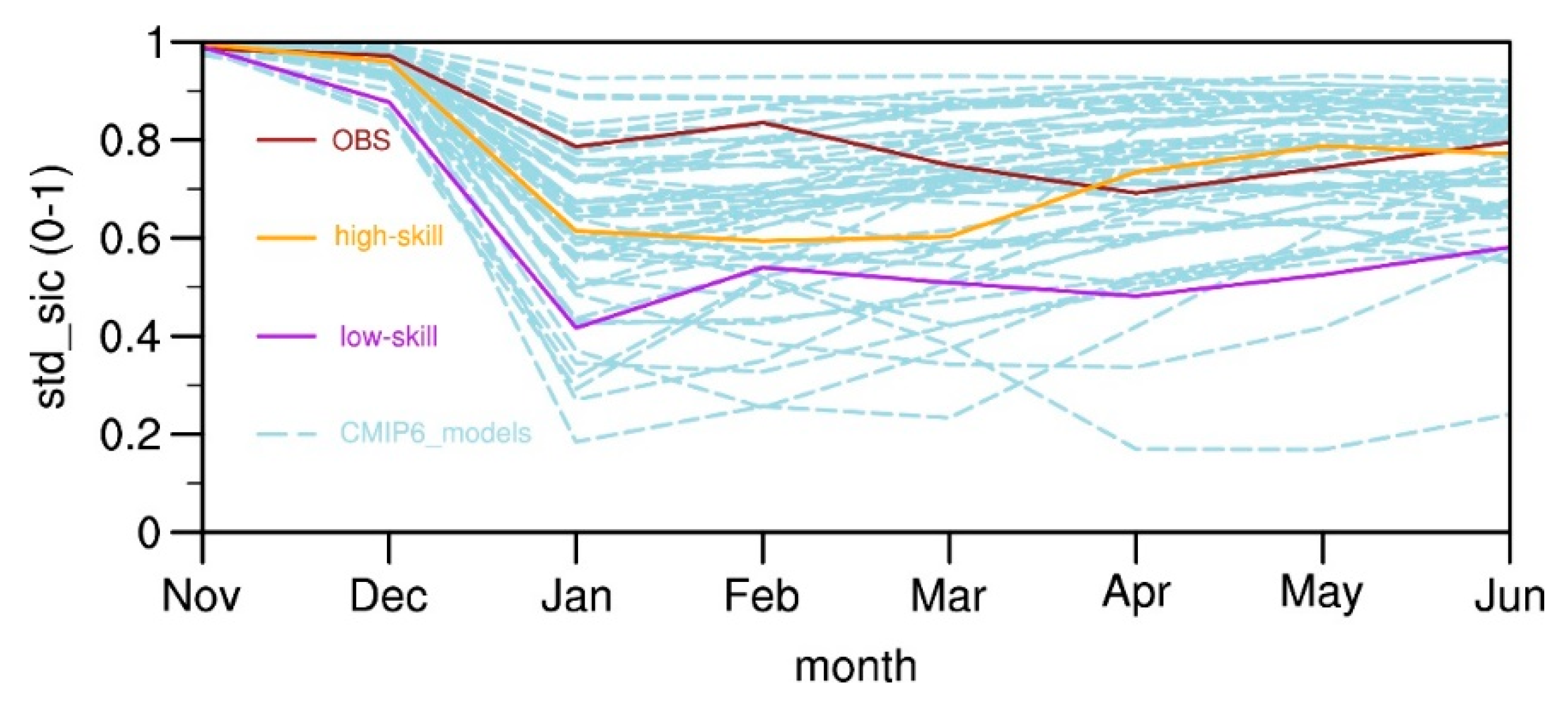
The evolution of the regressed standardized monthly Arctic SIC anomalies in the Kara–Barents Seas from early winter to early summer against the bimonthly (November–December mean) SIC index is shown in Figure 6 for the observations, individual models, low-skill MME, and high-skill MME. In the observations, the standard deviation of the Barents–Kara SIC in November and December exceeds 0.90. For a unit SIC change in early winter (~0.1), this value decreases to 0.8 units in January and February, and further decreases to 0.7 units in March and April, but recovers somewhat to ~0.8 units in May and June. CMIP6 models simulate the SIC anomalies with different degrees of success. In general, most CMIP6 models could simulate the gradually decreased Arctic SIC anomalies. Specifically, individual models (dash), high-skill MME (solid yellow), and low-skill MME (solid purple) display different reproducibility of the SIC persistency. Compared with low-skill MME, high-skill MME is much closer to the observations, especially after April when SIC anomalies remain stable. The reproduction of high-skill MME and low-skill MME from November to June is consistent with Figure 5a–e.

3.3.2. Atmospheric Circulation Changes Associated with Sea Ice Forcing

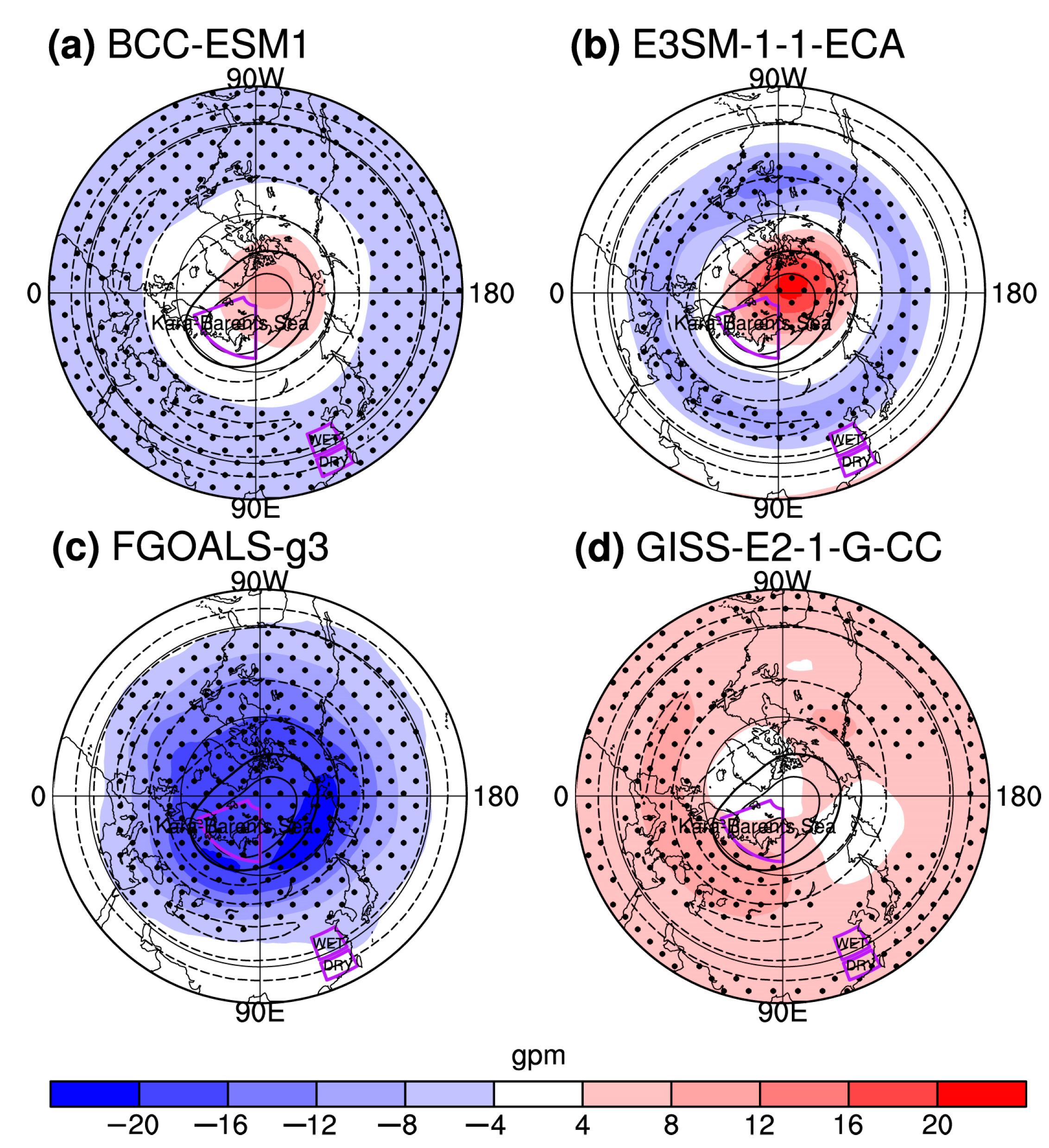
Figure 7 shows the regressed stratospheric anomalies in May and June against the November–December Barents–Kara sea ice for two representative high-skill models (BCC-ESM1 and E3SM1-1-ECA) and two low-skill models (FGOALS-g3 and GISS-E2-1-G-CC) compared with the ERA5 reanalysis (see the contours). Based on the reanalysis, negative height anomalies prevail at mid-latitudes, while positive height anomalies form over the Arctic Ocean. This dipole structure in early summer resembles the negative phase of NAM, which is opposite to the stratospheric response to the Barents–Kara sea ice forcing in winter [20,26]. This negative NAM pattern is well simulated by the two high-skill models, although the anomaly amplitude at midlatitudes is weaker than in ERA5 (Figure 7a,b). In contrast, the circulation pattern in low-skill models is far biased from ERA5 (Figure 7c,d). FGOALS-g3 simulates negative geopotential height anomalies in middle and high latitudes, the observed positive height anomalies in higher latitudes are missing for this model. GISS-E2-1-G-CC reproduces a positive height anomalies pattern. Overall, high-skill models reproduce the reversed NAM mode obviously, but low-skill models fail.
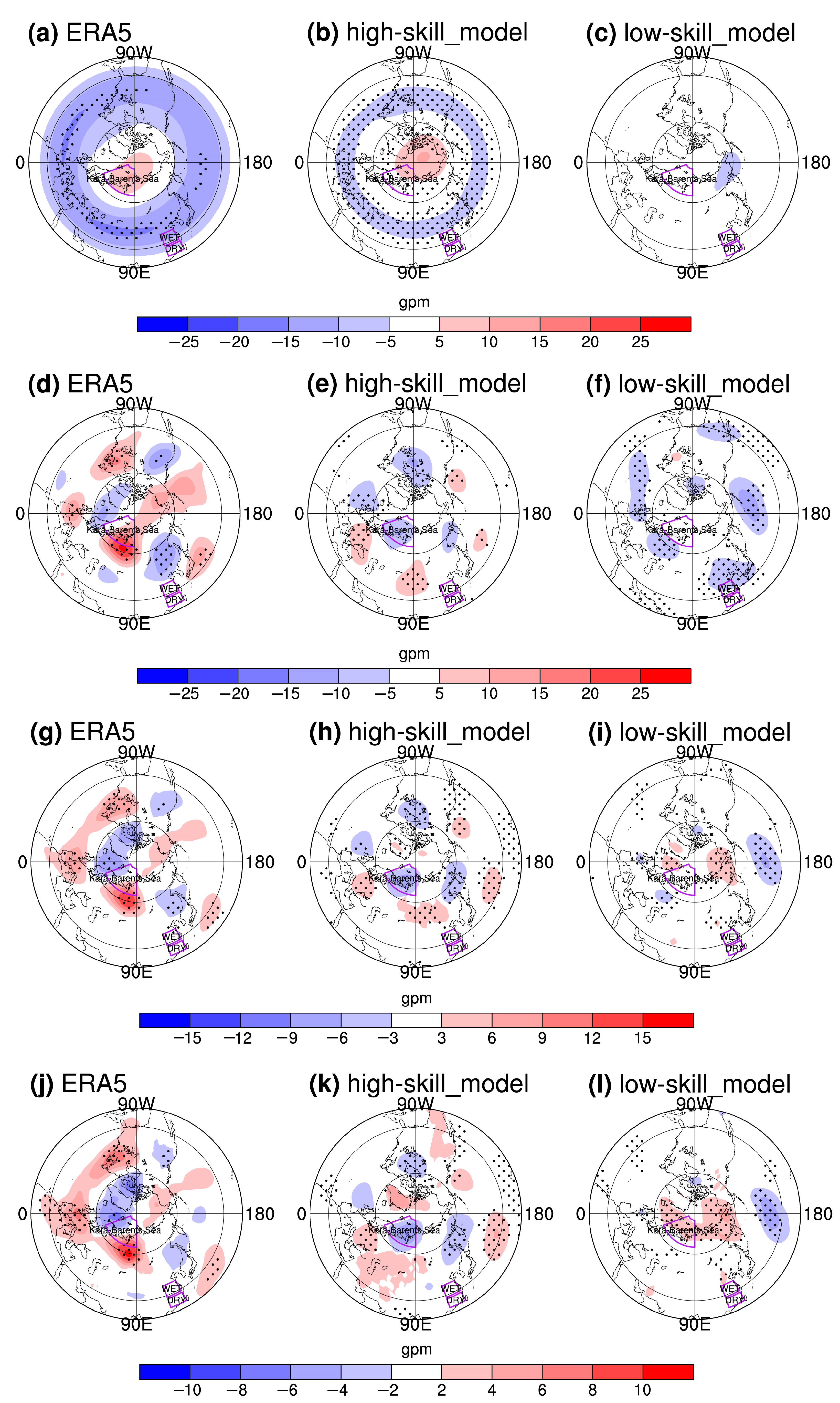
To examine the stratosphere−troposphere coupling associated with the sea ice forcing, Figure 8 shows the lagged regression of the height anomalies in the stratosphere and troposphere. In the reanalysis, a negative Northern Annular Mode (NAM) pattern (i.e., Arctic geopotential height anomalies are contrasted with mid-latitude annular height anomalies in a dipole pattern) appears in the stratosphere and develops downward (left column of Figure 8). Specifically, positive height anomalies prevail over the Arctic, while a negative height anomaly band forms at midlatitudes in the troposphere. The zonal symmetry in the stratosphere is much more evident in the stratosphere than in the troposphere. However, the tropospheric circulation anomalies have several centers at 200 hPa spanning from Barents–Kara Seas, central Asia, Northeast China to Japan (Figure 8d). This wave train-like response pattern is likely induced by the sea ice forcing directly [62,63]. These centers are also clearly present at 700 hPa, but shifted a little southward (Figure 8g); northern China is controlled by the anomalous low, and South China is controlled by the anomalous high spanning from the sea to south of Japan. The circulation anomalies in the troposphere in May and June are affected both by the downward impact of the stratosphere (zonal symmetry) and by the direct sea ice forcing (wave train-like pattern with zonal asymmetry), which has a long memory since the preceding early winter.
The observed negative NAM pattern in the stratosphere is well reproduced by representative high-skill models, and the stratosphere−troposphere coupling is also well simulated (middle column of Figure 8). As in the reanalysis, positive height anomalies appear over the Arctic, and a negative height anomaly band develops at the mid-latitudes. Furthermore, for the entire troposphere, an anomalous high develops in the downstream of Barents–Kara Seas, and a negative height center forms over Northeast Asia (Figure 8d,g,j). The wave train-like circulation pattern in high-skill models nearly replicates the reanalysis, except that the two centers shift somewhat eastward. In contrast, low-skill models fail to simulate the negative NAM-like pattern in the stratosphere. The tropospheric circulation anomalies in low-skill models are also not well simulated (right column of Figure 8), and the wave train-like response pattern is even reversed as compared with the reanalysis (Figure 8i,l). Overall, the poor reproducibility of the circulation anomalies, especially in the upper troposphere and lower stratosphere associated with the SIC forcing by low-skill models, is consistent with the underestimation of the sea ice variability. The circulation anomalies associated with SIC forcing are better simulated by high-skill models (middle column of Figure 8). The high-skill MMEs in Figure 8 simulate the stratospheric response well, which is consistent with the more realistic precipitation anomaly patterns in Figure 3. Low-skill models simulate unreal stratospheric responses, and the regressed rainfall anomaly pattern is even reversed. Yang et al. [20] showed that the anomalous northerlies in the west of the cyclone over the East China Sea converge with the anomalous southwesterlies in Yangtze–Huai Rivers Valley in the lower troposphere (at 700 hPa and 850 hPa), explaining the wet anomalies to the north of Yangtze River in June well.
The stratospheric polar vortex plays an important role in stratosphere−troposphere coupling [64,65,66]. The lead/lag regression of the circumpolar zonal winds against the standardized SIC index in Barents–Kara Seas is shown in Figure 9 for the reanalysis and several representative models. Following anomalous sea ice growth in early winter, the intensity of the stratospheric polar vortex is enhanced in winter, corresponding to the strengthening of the height meridional gradient in the circumpolar region and the development of circumpolar westerly anomalies (Figure 9a). The westerly anomalies are maximized in January and show an evident downward propagation. However, the circulation anomalies reverse the sign in spring. A weak stratospheric polar vortex is usually accompanied with active planetary waves, and active dynamics in early winter gradually change the mean state, which is followed by inactive waves and a strong polar vortex in spring, and vice versa [67]. Therefore, the reversal of the stratospheric NAM and the long memory of the sea ice itself collaborate to influence the China climate.
The MME of high-skill models simulates the positive NAM in winter and negative NAM in spring–early summer well (Figure 9b). The reversal of NAM is clearly present in the high-skill models, highly resembling the reanalysis, except that the geopotential anomalies in May and June are inconsistent above 10 hPa. In contrast, the MME of low-skill models struggles to simulate the negative NAM-like response in spring–early summer (Figure 9c). As a consequence, the downward propagation of stratospheric signals is absent in low-skill models.

4. Discussion

The MME for high-skill models better simulates the SIC memory and stratospheric variability than the MME for low-skill models. A previous study indicated that the lack of stratospheric variability in the low top models may increase biases in the stratosphere−tropospheric coupling simulations [47], whereas there is no clear evidence that an obvious gap exists in the simulation between high-top and low-top models in this study. The too-short memory of the SIC in most models with a poor self-persistence in Barents–Kara Seas leads to an unrealistic atmospheric response to SIC, but high-skill models simulate better than low-skill models in this pathway. An increase in the Arctic SIC over Barents–Kara Seas is followed by weakened planetary waves and a strong stratospheric polar vortex in winter [20]. Previous studies have reported that Arctic sea ice loss over Barents–Kara Seas usually corresponds to a weakened stratospheric polar vortex [26,56,68]. However, the reversal of the stratospheric NAM associated with the Arctic SIC forcing is not widely reported. The impact of the Arctic SIC on China rainfall is also very different in winter and summer (not shown), which might be related to the reversed phase of NAM.
High-skill models and their MME show a longer SIC memory, a more reasonable stratospheric variability, and a better tropospheric wave train-like circulation, and thus a more realistic rainfall anomaly dipole in eastern China. However, most CMIP6 models are not so skilled at simulating the linkage between Barents–Kara SIC in early winter and rainfall in early summer, and biases are complicated and different for models. Biases in the mean state of the Arctic SIC, overestimation of the covariance of SIC across different regions in the Arctic, and the errors in rainfall and circulation can lead to the loss of this observed link in CMIP6 models. Because of the poor performance of CMIP6 models in simulating the teleconnection associated with Arctic SIC forcing, especially the stratospheric pathway, projection of the future climatic change associated with SIC variability is still a challenge for the scientific community.
Considering that the maximum coupling appears when Barents–Kara sea ice leads to eastern China rainfall by nearly half a year, and that the sea ice has a long memory, the sea ice state is still a potential predictor for China rainfall prediction. There are also other possible teleconnection routes for SIC forcings such as strengthened blockings, increased cyclones, and the warm Arctic−cold Eurasia pattern, which is beyond the scope of the paper and left for future investigation [13,61].

5. Conclusions

In our previous study, we revealed the possible lagged impact of SIC forcing in Barents–Kara Seas in early winter on China rainfall in early summer. This study is aimed to assess the general performance of CMIP6 models in reproducing this linkage between the Barents–Kara sea ice and China rainfall in two populated regions. The main biases in the mean state and variability of the Arctic sea ice and the SIC–China rainfall linkage are evaluated. The main findings of this study are as follows.
Most CMIP6 models show the potential for overestimating the Arctic SIC (Figure 1 and Figure 2); the SIC variability simulated by low-skill models and their MME in Barents–Kara Seas in early winter is weaker than that in the observations. The largest errors appear in the edge area of the Arctic sea ice, and high-skill models with a better reproducibility of the SIC mean state also present more realistic SIC variability in Barents–Kara Seas. MMEs for the high-top and low-top models show some, but insignificant, differences in SIC climatology and variability. In addition, the sea ice model component plays a dominant role in the simulation of SIC.
A few high-skill models with reasonable simulation of SIC variability in winter can generally reproduce the rainfall anomaly dipole in China in early summer. As in the observations, high-skill models simulate a wet band in Southern China and a dry band to the north of the Yangtze River, although the rainfall anomaly amplitude is underestimated. In contrast, low-skill models simulate a rainfall anomaly pattern either opposite to the observations or illusively monopole. Selected typical CMIP6 models quantitatively reproduce the lagged relationship between Barents–Kara sea ice and June rainfall in South China. Four representative models (high-skill models: BCC-ESM1 and CAMS-CSM1-0; low-skill models: CAS-ESM2-0 and GISS-E2-1-G-CC) quantitatively reproduce the relationship between Barents–Kara sea ice and June rainfall to the north of Yangtze River.
The lagged impact of Barents–Kara SIC in winter on China rainfall is due to the long memory of the sea ice. The observed SIC anomalies in early winter can last to the following summer, which weakens in spring but is reinforced in early summer. High-skill models capture the long memory of the Barents–Kara SIC, which also weakens in spring, but redevelops in summer. However, low-skill models can reasonably simulate the SIC anomalies in Barents–Kara Seas in early and late winter, but they disappear more rapidly in spring and fail to reinforce in early summer. The relatively short memory of the SIC in low-skill models partially explain the underrepresentation of the Arctic SIC–China climate relationship, although causes for the SIC memory in CMIP6 models and complex and still not well understood, and have been left for future studies. The SIC forcing in early summer can lead to concurrent circulation change and finally affect China rainfall.
A negative stratospheric NAM like pattern is observed in early summer, which is opposite to the positive NAM response in winter to the increased SIC forcing in Barents–Kara Seas [20]. Arctic SIC forcing leads to a subsequent lagged stratospheric response, which can also impact the tropospheric circulation again in spring and early summer via the stratosphere–troposphere coupling. The negative NAM-like response in early summer develops from the stratosphere to troposphere, corresponding to an anomalous high over the Arctic and a low band at mid-latitudes. Furthermore, a wave train-like anomaly pattern spans from downstream of Barents–Kara Seas to central Asia, Northeast China, Japan, and the Pacific Ocean. Some studies also indicate that mid-to-high latitudes may play a role in bridging the SIC forcing and China climate variations [69,70]. The weakened zonal wind provides a favorable dynamic condition for the development of a high-latitude ridge around the Ural Mountain [69,70]. The anomalous low in the north and the anomalous high in the south of China are consistent with the rainfall anomaly dipole. High-skill models capture the stratosphere−troposphere coupling in early summer and the wave train-like circulation pattern in the troposphere. However, most CMIP6 models underrepresent the stratosphere−troposphere coupling following SIC variability in Barents–Kara Seas, and the wave train-like pattern is also absent, which is likely related to the more rapid disappearance of the simulated SIC anomaly forcing.
The observed downward propagation of the stratospheric NAM signals is well simulated in the representative high-skill models. Accelerated westerlies develop in winter, which show a downward impact in winter and spring. The reversal of the circumpolar wind anomalies occurs in spring, which propagate downward to the troposphere in early summer. High-skill models capture this reversal and the tropospheric circulation changes via the stratospheric pathway. However, most CMIP6 models fail to simulate the stratospheric pathway, which further increase the biases in the simulation of the SIC–China climate linkage.
This paper and our previous study have confirmed the teleconnection from the Arctic to midlatitudes and from early winter to early summer. The importance of stratospheric pathway in bridging Arctic SIC variability and eastern China rainfall in summer needs further investigation. Furthermore, causes for the underrepresentation of the SIC−China climate linkage should be explored in the future.

Author Contributions

Conceptualization, J.R. and H.C.; methodology, H.Y. and H.C.; software, J.R. and H.C.; validation, J.R. and H.C.; formal analysis, G.W. and J.R.; investigation, H.Y. and H.C.; writing—original draft preparation, H.C. and G.W.; writing—review and editing, J.R. and J.L.; visualization, H.C.; supervision, J.R. and J.L.; project administration, H.Y. and J.R. All of the authors have read and agreed to the published version of the manuscript.

Funding

This work is supported by the National Natural Science Foundation of China (grant nos. 42030605 and 42175069), the Qinglan Project of Jiangsu of China, the College Students’ Practice Innovation Training Program of Jiangsu Province, NUIST Students’ Platform for Innovation and Entrepreneurship Training Program (Project 202310300071Y).

Data Availability Statement

The CMIP6 simulations are available through ESGF (https://esgf-node.llnl.gov/projects/esgf-llnl/) (accessed on 1 April 2022). We also acknowledge ECMWF for providing three modern reanalyses (ERA5). ERA5 is available from https://cds.climate.copernicus.eu/. Arctic sea ice concentration data are freely available from UK Met Office (https://www.metoffice.gov.uk/hadobs/hadisst/data/download.html) (accessed on 1 April 2022). CMAP and GPCC (https://psl.noaa.gov/data/gridded/data.cmap.html) precipitation data are provided by the NOAA/OAR/ESRL PSL (accessed on 1 April 2022).

Acknowledgments

We thank ESGF, ECMWF, UKMO, and NOAA for their providing the datasets.

Conflicts of Interest

The authors declare no conflict of interest.

References

  1. Screen, J.A.; Simmonds, I. The central role of diminishing sea ice in recent Arctic temperature amplification. Nature 2010, 464, 1334–1337. [Google Scholar] [CrossRef] [PubMed] [Green Version]
  2. Serreze, M.C.; Barry, R.G. Processes and impacts of arctic amplification: A research synthesis. Glob. Planet. Chang. 2011, 77, 85–96. [Google Scholar] [CrossRef]
  3. Mysak, L.A.; Venegas, S.A. Decadal climate oscillations in the Arctic: A new feedback loop for atmosphere-ice-ocean interactions. Geophys. Res. Lett. 1998, 25, 3607–3610. [Google Scholar] [CrossRef]
  4. He, J.; Li, Q.; Wu, F. Arctic sea ice declining and its impact on the cold Eurasian winters: A review. Adv. Earth Sci. 2014, 29, 913–921. [Google Scholar] [CrossRef]
  5. He, J.H.; Wu, F.M.; Qi, L. Decadal/Interannual linking between autumn Arctic sea ice and following winter Eurasian air temperature. Chin. J. Geophys. 2015, 58, 1089–1102. [Google Scholar] [CrossRef]
  6. Ding, S.Y.; Wu, B.Y. Linkage between Autumn sea ice loss and ensuing spring Eurasian temperature. Clim. Dyn. 2021, 57, 2793–2810. [Google Scholar] [CrossRef]
  7. Bushuk, M.; Msadek, R.; Winton, M.; Vecchi, G.A.; Gudgel, R.; Rosati, A.; Yang, X.S. Summer enhancement of Arctic sea ice volume anomalies in the September-ice zone. J. Clim. 2017, 30, 2341–2362. [Google Scholar] [CrossRef] [Green Version]
  8. Pithan, F.; Mauritsen, T. Arctic amplification dominated by temperature feedbacks in contemporary climate Models. Nat. Geosci. 2014, 7, 181–184. [Google Scholar] [CrossRef]
  9. Wu, F.; Li, W.; Li, W. Causes of Arctic amplification: A review. Adv. Earth Sci. 2019, 34, 232–242. [Google Scholar] [CrossRef]
  10. Cohen, J.; Zhang, X.; Francis, J.; Jung, T.; Kwok, R.; Overland, J.; Ballinger, T.J.; Bhatt, U.S.; Chen, H.W.; Coumou, D.; et al. Divergent consensuses on Arctic amplification influence on midlatitude severe winter weather. Nat. Clim. Chang. 2020, 10, 20–29. [Google Scholar] [CrossRef]
  11. Francis, J.A.; Vavrus, S.J. Evidence linking Arctic amplification to extreme weather in mid-latitudes. Geophys. Res. Lett. 2012, 36, 136–157. [Google Scholar] [CrossRef]
  12. Warner, J.L.; Screen, J.A.; Scaife, A.A. Links between Barents-Kara sea ice and the extratropical atmospheric circulation explained by internal variability and tropical forcing. Geophys. Res. Lett. 2020, 47, e2019GL085679. [Google Scholar] [CrossRef]
  13. Wang, S.; Nath, D.; Chen, W.; Ma, T. CMIP5 model simulations of warm Arctic-cold Eurasia pattern in winter surface air temperature anomalies. Clim. Dyn. 2020, 54, 4499–4513. [Google Scholar] [CrossRef]
  14. Honda, M.; Inoue, J.; Yamane, S. Influence of low Arctic sea-ice minima on anomalously cold Eurasian winters. Geophys. Res. Lett. 2009, 36, L08707. [Google Scholar] [CrossRef]
  15. Petoukhov, V.; Semenov, V.A. A Link between reduced Barents-Kara sea ice and cold winter extremes over northern continents. J. Geophys. Res. Atmos. 2010, 115, D21111. [Google Scholar] [CrossRef]
  16. Ding, S.Y.; Wu, B.Y.; Chen, W. Dominant characteristics of early autumn Arctic sea ice variability and its impact on winter Eurasian climate. J. Clim. 2021, 34, 1825–1846. [Google Scholar] [CrossRef]
  17. Guo, D.; Gao, Y.Q.; Bethke, I.; Gong, D.Y.; Johannessen, O.M.; Wang, H.J. Mechanism on how the spring Arctic sea ice impacts the east Asian summer monsoon. Theor. Appl. Climatol. 2014, 115, 107–119. [Google Scholar] [CrossRef]
  18. Xie, Y.K.; Liu, Y.Z.; Huang, J.P. The influence of the autumn Arctic sea ice on winter air temperature in China. Acta Meteorol. Sin. 2014, 72, 703–710. [Google Scholar] [CrossRef]
  19. Zhu, Z.; Huang, F.; Xie, X. Predictability of Chinese summer extreme rainfall based on Arctic sea ice and tropical sea surface temperature. J. Ocean Univ. China 2019, 18, 626–632. [Google Scholar] [CrossRef]
  20. Yang, H.; Rao, J.; Chen, H. Possible lagged impact of the Arctic sea ice in Barents–Kara seas on June precipitation in Eastern China. Front. Earth Sci. 2022, 10, 886192. [Google Scholar] [CrossRef]
  21. Zhao, P.; Zhang, X.; Zhou, X.; Ikeda, M.; Yin, Y. The sea ice extent anomaly in the north Pacific and its impact on the east Asian summer monsoon rainfall. J. Clim. 2004, 17, 3434–3447. [Google Scholar] [CrossRef]
  22. Wu, B.Y.; Zhang, R.H.; Wang, B. On the association between spring Arctic sea ice concentration and Chinese summer rainfall: A further study. Adv. Atmos. Sci. 2009, 26, 666–678. [Google Scholar] [CrossRef]
  23. Shen, H.B.; He, S.P.; Wang, H.J. Effect of summer Arctic sea ice on the reverse August precipitation anomaly in eastern China between 1998 and 2016. J. Clim. 2019, 32, 3389–3407. [Google Scholar] [CrossRef]
  24. Zhang, R.N.; Zhang, R.H.; Zuo, Z.Y. Impact of Eurasian spring snow decrement on east Asian summer precipitation. J. Clim. 2017, 30, 3421–3437. [Google Scholar] [CrossRef]
  25. Deser, C.; Tomas, R.A.; Sun, L.T. The role of ocean-atmosphere coupling in the zonal-mean atmospheric response to Arctic sea ice loss. J. Clim. 2015, 28, 2168–2186. [Google Scholar] [CrossRef] [Green Version]
  26. Kim, B.M.; Son, S.W.; Min, S.K.; Jeong, J.H.; Kim, S.J.; Zhang, X.D.; Shim, T.; Yoon, J.H. Weakening of the stratospheric polar vortex by Arctic sea-ice Loss. Nat. Commun. 2014, 5, 4646. [Google Scholar] [CrossRef] [Green Version]
  27. Sun, L.T.; Deser, C.; Polvani, L.; Tomas, R. Influence of projected Arctic sea ice loss on polar stratospheric ozone and Circulation in Spring. Environ. Res. Lett. 2014, 9, 084016. [Google Scholar] [CrossRef]
  28. Cai, D.; Dameris, M.; Garny, H.; Runde, T. Implications of all season Arctic sea-ice anomalies on the stratosphere. Atmos. Chem. Phys. 2012, 12, 11819–11831. [Google Scholar] [CrossRef] [Green Version]
  29. Sun, L.T.; Deser, C.; Tomas, R.A. Mechanisms of stratospheric and tropospheric circulation response to projected Arctic sea ice loss. J. Clim. 2015, 28, 7824–7845. [Google Scholar] [CrossRef]
  30. Tang, Q.H.; Zhang, X.J.; Yang, X.H.; Francis, J.A. Cold winter extremes in northern continents linked to Arctic sea ice loss. Environ. Res. Lett. 2013, 8, 014036. [Google Scholar] [CrossRef]
  31. Sui, C.J.; Zhang, Z.H.; Yu, L.J.; Li, Y.; Song, M.R. Sensitivity and nonlinearity of Eurasian winter temperature response to recent Arctic sea ice loss. Acta Oceanol. Sin. 2017, 36, 52–58. [Google Scholar] [CrossRef]
  32. Cohen, J.; Screen, J.A.; Furtado, J.C.; Barlow, M.; Whittleston, D.; Coumou, D.; Francis, J.; Dethloff, K.; Entekhabi, D.; Overland, J.; et al. Recent arctic amplification and extreme mid-latitude weather. Nat. Geosci. 2014, 7, 627–637. [Google Scholar] [CrossRef] [Green Version]
  33. Overland, J.E.; Wang, M.Y. Increased variability in the early winter subarctic north American Atmospheric Circulation. J. Clim. 2015, 28, 7297–7305. [Google Scholar] [CrossRef]
  34. Hoshi, K.; Ukita, J.; Honda, M.; Nakamura, T.; Yamazaki, K.; Miyoshi, Y.; Jaiser, R. Weak stratospheric polar vortex events modulated by the Arctic sea-ice loss. J. Geophys. Res. Atmos. 2019, 124, 858–869. [Google Scholar] [CrossRef] [Green Version]
  35. Kretschmer, M.; Zappa, G.; Shepherd, T.G. The role of Barents–Kara sea ice loss in projected polar vortex changes. Weather Clim. Dyn. 2020, 1, 715–730. [Google Scholar] [CrossRef]
  36. Stroeve, J.C.; Kattsov, V.; Barrett, A.; Serreze, M.; Pavlova, T.; Holland, M.; Meier, W. Trends in Arctic sea ice extent from CMIP5, CMIP3 and observations. Geophys. Res. Lett. 2012, 39, L16502. [Google Scholar] [CrossRef] [Green Version]
  37. Knutti, R.; Masson, D.; Gettelman, A. Climate Model Genealogy: Generation CMIP5 and how we got there. Geophys. Res. Lett. 2013, 40, 1194–1199. [Google Scholar] [CrossRef]
  38. Chu, M.; Shi, X.; Fang, Y.; Zhang, L.; Wu, T.; Zhou, B. Impacts of SIS and CICE as sea ice components in BCC_CSM on the simulation of the Arctic climate. J. Ocean Univ. China 2019, 18, 553–562. [Google Scholar] [CrossRef]
  39. Stroeve, J.; Holland, M.M.; Meier, W.; Scambos, T.; Serreze, M. Arctic sea ice decline: Faster than forecast. Geophys. Res. Lett. 2007, 34, L09501. [Google Scholar] [CrossRef]
  40. Rayner, N.A.; Parker, D.E.; Horton, E.B.; Folland, C.K.; Alexander, L.V.; Rowell, D.P.; Kent, E.C.; Kaplan, A. Global analyses of sea surface temperature, sea ice, and night marine air temperature since the late nineteenth century. J. Geophys. Res. Atmos. 2003, 108, 4407. [Google Scholar] [CrossRef] [Green Version]
  41. Hersbach, H.; Bell, B.; Berrisford, P.; Hirahara, S.; Horanyi, A.; Munoz-Sabater, J.; Nicolas, J.; Peubey, C.; Radu, R.; Schepers, D.; et al. The ERA5 global reanalysis. Q. J. R. Meteorol. Soc. 2020, 146, 1999–2049. [Google Scholar] [CrossRef]
  42. Xie, P.; Arkin, P.A. Global Precipitation: A 17-year monthly analysis based on gauge observations, satellite estimates, and numerical model outputs. Bull. Am. Meteorol. Soc. 1997, 78, 2539–2558. [Google Scholar] [CrossRef]
  43. Schneider, U.; Becker, A.; Finger, P.; Meyer-Christoffer, A.; Ziese, M.; Rudolf, B. GPCC’s new land surface precipitation climatology based on quality-controlled in situ data and its role in quantifying the global water cycle. Theor. Appl. Climatol. 2013, 115, 15–40. [Google Scholar] [CrossRef] [Green Version]
  44. Meehl, G.A.; Covey, C.; Delworth, T.; Latif, M.; Mcavaney, B.; Mitchell, J.F.B.; Stouffer, R.J.; Taylor, K.E. The WCRP CMIP3 multimodel dataset: A new era in climate change research. Bull. Am. Meteorol. Soc. 2007, 88, 1383–1394. [Google Scholar] [CrossRef] [Green Version]
  45. Taylor, K.E.; Stouffer, R.J.; Meehl, G.A. An overview of CMIP5 and the experiment design. Bull. Am. Meteorol. Soc. 2012, 93, 485–498. [Google Scholar] [CrossRef] [Green Version]
  46. Eyring, V.; Bony, S.; Meehl, G.A.; Senior, C.A.; Stevens, B.; Stouffer, R.J.; Taylor, K.E. Overview of the Coupled model intercomparison project phase 6 (CMIP6) experimental design and organization. Geosci. Model Dev. 2016, 9, 1937–1958. [Google Scholar] [CrossRef] [Green Version]
  47. Charlton-Perez, A.J.; Baldwin, M.P.; Birner, T.; Black, R.X.; Butler, A.H.; Calvo, N.; Davis, N.A.; Gerber, E.P.; Gillett, N.; Hardiman, S. On the lack of stratospheric dynamical variability in low-top versions of the CMIP5 models. J. Geophys. Res. Atmos. 2013, 118, 2494–2505. [Google Scholar] [CrossRef] [Green Version]
  48. Rao, J.; Garfinkel, C.I.; Wu, T.; Lu, Y.; Chu, M. Mean state of the northern hemisphere stratospheric polar vortex in three generations of CMIP models. J. Clim. 2022, 35, 4603–4625. [Google Scholar] [CrossRef]
  49. Onarheim, I.H.; Eldevik, T.; Smedsrud, L.H.; Stroeve, J.C. Seasonal and regional manifestation of Arctic sea ice loss. J. Clim. 2018, 31, 4917–4932. [Google Scholar] [CrossRef]
  50. Ringgaard, I.M.; Yang, S.T.; Kaas, E.; Christensen, J.H. Barents-Kara sea ice and European winters in EC-Earth. Clim. Dyn. 2020, 54, 3323–3338. [Google Scholar] [CrossRef] [Green Version]
  51. Liptak, J.; Strong, C. The winter atmospheric response to sea ice anomalies in the Barents sea. J. Clim. 2014, 27, 914–924. [Google Scholar] [CrossRef]
  52. Woollings, T.; Harvey, B.; Masato, G. Arctic warming, atmospheric blocking and cold European winters in CMIP5 models. Environ. Res. Lett. 2014, 9, 014002. [Google Scholar] [CrossRef]
  53. Lu, C.; Li, K.; Xie, S.; Wang, Z.; Qin, Y. Month-to-month variability of autumn sea ice in the Barents and Kara seas and its relationship to winter air temperature in China. Adv. Meteorol. 2019, 2019, 4381438. [Google Scholar] [CrossRef] [Green Version]
  54. Long, Z.; Perrie, W. Changes in ocean temperature in the Barents sea in the twenty-first century. J. Clim. 2017, 30, 5901–5921. [Google Scholar] [CrossRef]
  55. Li, F.; Wang, H.; Gao, Y. Change in sea ice cover is responsible for non-uniform variation in winter temperature over east Asia. Atmos. Ocean. Sci. Lett. 2015, 8, 382. [Google Scholar] [CrossRef]
  56. Jaiser, R.; Dethloff, K.; Handorf, D. Stratospheric response to Arctic sea ice retreat and associated planetary wave propagation changes. Tellus A 2013, 65, 19375. [Google Scholar] [CrossRef] [Green Version]
  57. Zhang, R.N.; Sun, C.H.; Zhang, R.H.; Jia, L.W.; Li, W.J. The impact of arctic sea ice on the inter-annual variations of summer Ural blocking. Int. J. Climatol. 2018, 38, 4632–4650. [Google Scholar] [CrossRef]
  58. Coumou, D.; Lehmann, J.; Beckmann, J. The weakening summer circulation in the northern hemisphere mid-latitudes. Science 2015, 348, 324–327. [Google Scholar] [CrossRef]
  59. Lin, Z.D.; Li, F. Impact of interannual variations of spring sea ice in the Barents sea on east Asian rainfall in June. Atmos. Ocean. Sci. Lett. 2018, 11, 275–281. [Google Scholar] [CrossRef] [Green Version]
  60. Kelleher, M.E.; Ayarzagüena, B.; Screen, J.A. Interseasonal connections between the timing of the stratospheric final warming and Arctic sea ice. J. Clim. 2020, 33, 3079–3092. [Google Scholar] [CrossRef]
  61. Wang, S.; Nath, D.; Chen, W.; Wang, L. Recent strengthening of Greenland blocking drives summertime surface warming over northern Canada and eastern Siberia. J. Clim. 2019, 32, 3263–3278. [Google Scholar] [CrossRef]
  62. Fan, K. North pacific sea ice cover, a predictor for the western north Pacific typhoon frequency? Sci. China Earth Sci. 2007, 50, 1251–1257. [Google Scholar] [CrossRef]
  63. Wu, B.; Zhang, R.; D’arrigo, R.; Su, J. On the relationship between winter sea ice and summer atmospheric circulation over Eurasia. J. Clim. 2013, 26, 5523–5536. [Google Scholar] [CrossRef]
  64. Kodera, K.; Chiba, M.; Yamazaki, K.; Shibata, K.A. Possible influence of the polar night stratospheric jet on the subtropical tropospheric jet. J. Meteorol. Soc. Jpn. 2007, 69, 715–721. [Google Scholar] [CrossRef] [Green Version]
  65. Statnaia, I.; Karpechko, A.; Kämäräinen, M.; Järvinen, H. Stratosphere–troposphere coupling enhances subseasonal predictability of northern Eurasian cold spells. Q. J. R. Meteorol. Soc. 2022, 148, 2769–2783. [Google Scholar] [CrossRef]
  66. Perlwitz, J.; Graf, H.-F. Troposphere-stratosphere dynamic coupling under strong and weak polar vortex conditions. Geophys. Res. Lett. 2001, 28, 271–274. [Google Scholar] [CrossRef] [Green Version]
  67. Hu, J.; Ren, R.; Xu, H. Occurrence of winter stratospheric sudden warming events and the seasonal timing of spring stratospheric final warming. JAS. 2014, 71, 2319–2334. [Google Scholar] [CrossRef]
  68. Peings, Y.; Magnusdottir, G. Response of the wintertime northern hemisphere atmospheric circulation to current and projected arctic sea ice decline: A numerical study with CAM5. J. Clim. 2014, 27, 244–264. [Google Scholar] [CrossRef] [Green Version]
  69. Sun, C.; Yang, S.; Li, W.; Zhang, R.; Wu, R. Interannual variations of the dominant modes of East Asian winter monsoon and possible links to Arctic sea ice. Clim. Dyn. 2016, 47, 481–496. [Google Scholar] [CrossRef]
  70. Zhang, X.; Wu, B.; Ding, S. Influence of spring Arctic sea ice melt on Eurasian surface air temperature. Clim. Dyn. 2022, 59, 3305–3316. [Google Scholar] [CrossRef]
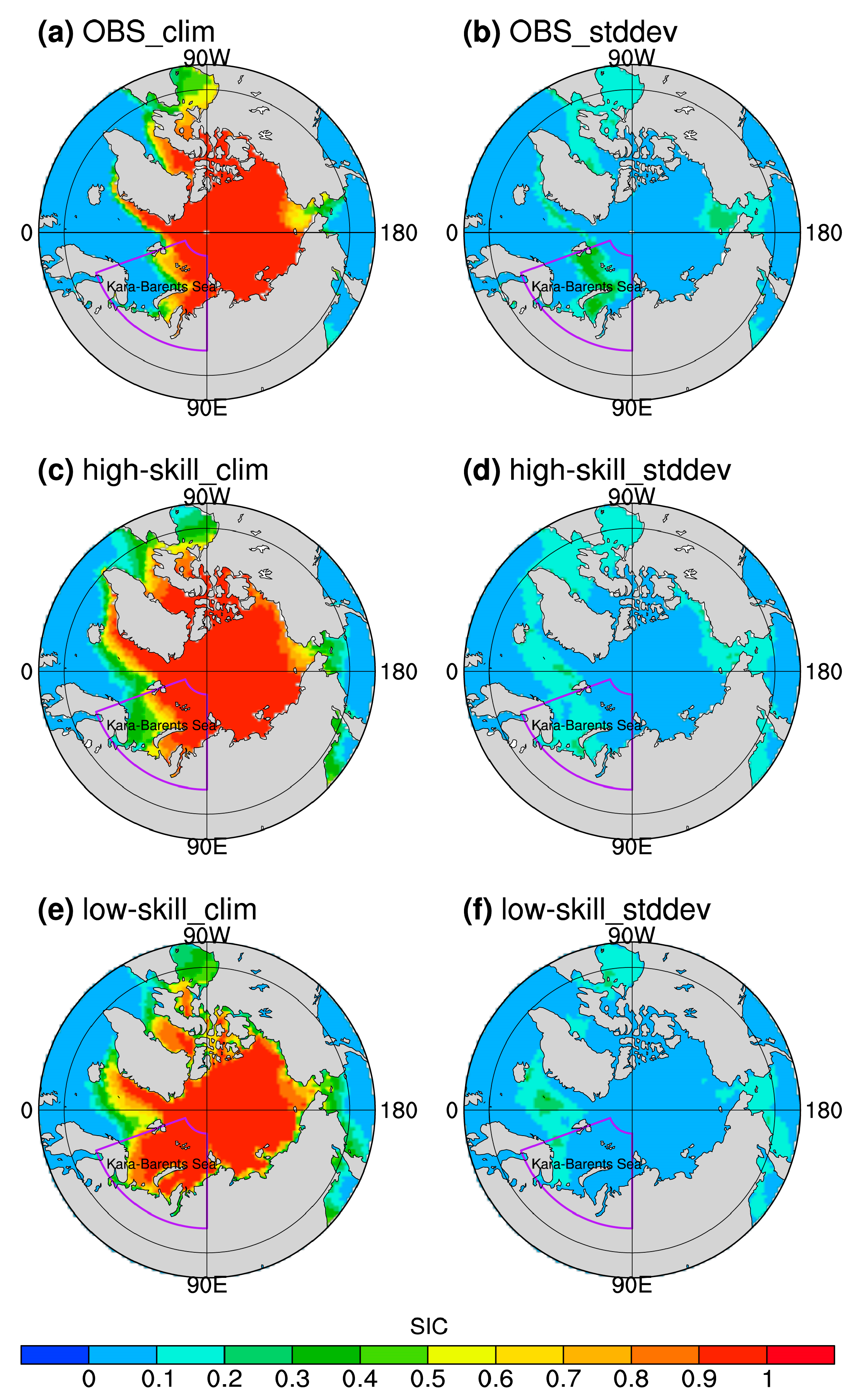
Figure 1. Climatology and variability of the Arctic sea ice cover in November and December from (a,b) Hadley Center sea ice concentration (SIC) observations, (c,d) multi-model ensemble mean (MME) for high-skill CMIP6 models, and (e,f) MME for low-skill CMIP6 models. The sector box marks Barents–Kara Seas where the variability is relatively large in the observations (65–85° N, 20–90° E).
Atmosphere 14 01044 g001
Figure 2. Climatology and standard deviation of SIC in Barents–Kara Seas in early winter for observations (1979–2020) and CMIP6 models (1973–2014). The error bar shows the standard deviation of the SIC for individual model (dark gray) or the inter-model standard deviation of the means for all CMIP6 models (dark purple: all models; dark red: high-top models; dark blue: low-top models). The horizontal black line is the climatology from observations, and the horizontal purple line and the purple bar are the MME for all models. High-top models and their MME are shown in red, and low-top models and their MME are shown in blue.
Atmosphere 14 01044 g002
Figure 3. Regression of June rainfall anomalies (units: mm) against the standardized early winter SIC in Barents–Kara Seas for (a,b) observations (CMAP and GPCC), (c,e,g) high-skill models MME and two representatives of high-skill CMIP6 models, and (d,f,h) low-skill models MME and two representatives of low-skill CMIP6 models. White/black dots mark the regression at the 95% confidence level (α = 0.05). The purple boxes show the relatively large variability centers (wetter region: 29–36° N, 110–120° E; drier region: 23–28° N, 110–120° E).
Atmosphere 14 01044 g003
Figure 4. Regression of June rainfall anomalies (units: mm) over two focused regions against standardized Arctic SIC in the Barents–Kara Seas in early winter for the observations (Hadley Center SIC and CMAP rainfall) and CMIP6 models. (a) Regression for South China. (b) Regression for the focused region to the north of the Yangtze River. The horizontal black line is the regression for observations as also shown in gray bars. The horizontal purple line and the purple bar are the MME for all models. High-top models and their MME are shown in red, and low-top models and their MME are shown in blue. The CMIP6 models with their names highlighted in purple show a rainfall anomaly dipole.
Atmosphere 14 01044 g004
Figure 5. Evolution of regressed Arctic SIC anomalies (units: dimensionless) from November–December to May–June against the standardized November–December mean SIC in Barents–Kara Seas (marked in the purple sector) for (a0–a3) observations, (b0–b3) high-skill MME, (c0–c3) low-skill MME, (d0–d3,e0–e3) representative high-skill models (BCC-ESM1 and E3SM-1-1-ECA) and (f0–f3,g0–g3) representative low-skill models (FGOALS-g3 and GISS-E2-1-G-CC). The black contours show the regression at the 95% confidence level.
Atmosphere 14 01044 g005
Figure 6. Regressed bimonthly Arctic SIC anomalies against the Barents−Kara SIC index in November–December for all CMIP6 models and the observations as a representation of the SIC persistency. CMIP6 models are shown in dashed lines, while the observation, high-skill MME and low-skill MME are shown in brown, yellow, and purple, respectively.
Atmosphere 14 01044 g006
Figure 7. Regression of geopotential height anomalies at 10 hPa (units: gpm) in May–June against the standardized November–December SIC index in Barents–Kara Seas (marked in the purple sector) for (a,b) two representative high-skill models and (c,d) two representative low-skill models. The dotted regions show the regression at a 95% confidence level. The contours show the regressed height anomalies based on ERA5 and HadISST.
Atmosphere 14 01044 g007
Figure 8. Regression of geopotential height anomalies (units: gpm) in May–June against the standardized SIC index in Barents–Kara Seas in early winter for ERA5 (left column, a,d,g,j), the MME of high-skill models (middle column, b,e,h,k), and the MME of low-skill models (right column, c,f,i,l). Four pressure levels are shown (top: 10 hPa; second row: 200 hPa; third row: 700 hPa; bottom: 850 hPa). The three parallel latitude circles are 20° N, 30° N, and 60° N, respectively. The dotted regions show the regression at a 90% confidence level.
Atmosphere 14 01044 g008
Figure 9. Lead/lag regression of circumpolar zonal wind anomalies at 60° N (contours; units: m/s) against the standardized SIC index in Barents–Kara Seas in early winter for (a) ERA5, (b) MME of typical high-skill models, and (c) MME of typical low-skill models. The shadings show the lead/lag correlation between the wind in November–June and the SIC index in early winter. The black contours show the regression at the 95% confidence level (r0.95 = 0.3 for DOF = 40; r0.95 = 0.16 for DOF = 150).
Atmosphere 14 01044 g009
Table 1. Brief information about the CMIP6 models used in this study.
AffiliationCMIP6 ID and NamesResolution (Models Top)Sea Ice Model
CSIRO, Australia(1) ACCESS-CM2N96L85 (85 km)CICE5.1.2
(2) ACCESS-ESM1-5N96L38 (39.2 km)CICE4.1
AWI, Germany(3) AWI-CM-1-1-MRT27L95 (80 km)FESOM 1.4
CMA BCC, China(4) BCC-CSM2-MRT106L46 (1.46 hPa)SIS2
(5) BCC-ESM1T42L26 (2.19 hPa)SIS2
CAMS, China(6) CAMS-CSM1-0T106L31 (10 hPa)SIS 1.0
(9) CAS-ESM2-0256 × 128L35 (2.2 hPa)CICE4
CCCMA, Canada(7) CanESM5T63L49 (1 hPa)LIM2
(8) CanESM5-CanOET63L49 (1 hPa)LIM2
NCAR,USA(10) CESM2F09L32 (2.25 hPa)CICE5.1
(11) CESM2-FV2F19L32 (2.25 hPa)CICE5.1
(12) CESM2-WACCMF9L70 (4.5 × 10⁻⁶ hPa)CICE5.1
(13) CESM2-WACCM-FV2F19L66 (4.5 × 10⁻⁶ hPa)CICE5.1
CMCC, Italy(14) CMCC-CM2-HR4288 × 192L26 (2 hPa)CICE4.0
(15) CMCC-ESM2288 × 192L30 (2 hPa)CICE4.0
CNRM, France(16) CNRM-CM6-1T127L91 (78.4 km)Gelato 6.1
(17) CNRM-ESM2-1T127L91 (78.4 km)Gelato 6.1
E3SM-Project,USA(18) E3SM-1-0F09L72 (0.1 hPa)MPAS-Sea ice
(19) E3SM-1-1F09L72 (0.1 hPa)MPAS-Sea ice
(20) E3SM-1-1-ECAF09L72 (0.1 hPa)MPAS-Sea ice
EC-Earth-Consortium, Europe(21) EC-Earth3-AerChemTL255L91 (0.01 hPa)LIM3
(22) EC-Earth3-CCTL255L91 (0.01 hPa)LIM3
(23) EC-Earth3-VegTL255L91 (0.01 hPa)LIM3
(24) EC-Earth3-Veg-LRTL159L62 (5 hPa)LIM3
CAS, China(25) FGOALS-f3-LC96L32 (2.16 hPa)CICE4.0
(26) FGOALS-g3180 × 80L26 (2.19 hPa)CICE4.0
FIO, China(27) FIO-ESM-2-0192 × 288L26 (2 hPa)CICE4.0
NOAA-GFDL, USA(28) GFDL-CM4C96L33 (1 hPa)GFDL-SIM4p25
(29) GFDL-ESM4C96L49 (0.01 hPa)GFDL-SIM4p5
NASA-GISS, USA(30) GISS-E2-1-G144 × 90L40 (0.1 hPa)GISS SI
(31) GISS-E2-1-G-CC144 × 90L40 (0.1 hPa)GISS SI
(32) GISS-E2-1-H144 × 90L40 (0.1 hPa)GISS SI
MOHC, UK(33) HadGEM3-GC31-LLN96L85 (85 km)CICE-HadGEM3-GSI8
(34) HadGEM3-GC31-MMN216L85 (85 km)CICE-HadGEM3-GSI8
INM, Russia(35) INM-CM4-8180 × 120L21 (10 hPa)INM-ICE1
(36) INM-CM5-0180 × 120L73 (0.2 hPa)INM-ICE1
IPSL, France(37) IPSL-CM6A-LRN96L79 (80 km)NEMO-LIM3
MIROC, Japan(38) MIROC6T85L81 (0.004 hPa)COCO4.9
(39) MIROC-ES2LT42L40 (3 hPa)COCO4.9
MPI, Germany(40) MPI-ESM1.2-HAMT63L47 (0.01 hPa)unnamed
(41) MPI-ESM1.2-LRT63L47 (0.01 hPa)unnamed
NUIST, China(42) NESMT63L47 (1 hPa)CICE4.1
(43) NorCPM1144 × 96L32 (2 hPa)CICE4
BCCR and NCC, Norway(44) NorESM2-LM144 × 96L32 (3 hPa)CICE
(45) NorESM2-MM288 × 192L32 (3 hPa)CICE
SNU, South Korea(46) SAM0-UNICON288 × 192L30 (2 hPa)CICE4.0
AS-RCEC, Taiwan, China(47) TaiESM1288 × 192L30 (2 hPa)CICE4
MOHC, UK(48) UKESM1-0-LLN96L85 (85 km)CICE-HadGEM3-GSI8
Disclaimer/Publisher’s Note: The statements, opinions and data contained in all publications are solely those of the individual author(s) and contributor(s) and not of MDPI and/or the editor(s). MDPI and/or the editor(s) disclaim responsibility for any injury to people or property resulting from any ideas, methods, instructions or products referred to in the content.