Application of a Deep Learning Fusion Model in Fine Particulate Matter Concentration Prediction

Abstract

With the rapid development of urbanization, ambient air pollution is becoming increasingly serious. Out of many pollutants, fine particulate matter (PM_2.5) is the pollutant that affects the urban atmospheric environment to the greatest extent. Fine particulate matter (PM_2.5) concentration prediction is of great significance to human health and environmental protection. This paper proposes a CNN-SSA-DBiLSTM-attention deep learning fusion model. This paper took the meteorological observation data and pollutant data from eight stations in Bijie from 1 January 2015 to 31 December 2022 as the sample data for training and testing. For the obtained data, the missing values and the data obtained from the correlation analysis performed were first processed. Secondly, a convolutional neural network (CNN) was used for the feature selection. DBILSTM was then used to establish a network model for the relationship between the input and actual output sequences, and an attention mechanism was added to enhance the impact of the relevant information. The number of units in the DBILSTM and the epoch of the whole network were optimized using the sparrow search algorithm (SSA), and the predicted value was the output after optimization. This paper predicts the concentration of PM_2.5 in different time spans and seasons, and makes a comparison with the CNN-DBILSTM, BILSTM, and LSTM models. The results show that the CNN-SSA-DBiLSTM-attention model had the best prediction effect, and its accuracy improved with the increasing prediction time span. The coefficient of determination (R²) is stable at about 0.95. The results revealed that the proposed CNN-SSA-DBiLSTM-attention ensemble framework is a reliable and accurate method, and verifies the research results of this paper in regard to the prediction of PM_2.5 concentration. This research has important implications for human health and environmental protection. The proposed method could inspire researchers to develop even more effective methods for atmospheric environment pollution modeling.

1. Introduction

In recent years, with the continuous acceleration of the industrialization process [1], China’s ecological and environmental pollution problems have become prominent [1,2]; air pollution is particularly prominent, and air pollutants, such as PM_2.5, have accumulated in large amounts [3], and these have received significant attention across society [4]. PM_2.5 is a form of fine particle with an aerodynamic diameter of <2.5 μm [5]; it is one of the main sources of air pollution in urban areas [6,7]. The sources of PM_2.5 include direct sources [8] and indirect sources [9]. The direct sources are particulate matter generated by pollution sources, such as smoke, particles from automobile exhaust emissions, and sand and soil formed by the wind force. The indirect source is the secondary pollution formed by the complex reactions of gases generated by the pollution sources in the air; for example, H₂S, SO₂, etc., discharged from a boiler are oxidized by the atmosphere to form sulfate particles. With the implementation of the “Air Pollution Prevention and Control Action Plan”, the PM_2.5 pollution problem in most cities in China has been alleviated [10], but PM_2.5 concentrations have not yet reached the national standard [11]. Therefore, the advanced prediction of PM_2.5 concentration could effectively prevent and reduce its harm to human beings.

At present, numerical prediction, statistical prediction, and artificial intelligence prediction are the three main prediction methods for predicting pollutants [12,13]. The first numerical prediction simulates the space–time distribution of air pollutants by adding pollution source data and meteorological data, and uses the WRF Chem model to predict surface air pollutants in East China [14,15]. Li et al. [16] introduced the idea of regional chemical transport on the basis of the CMAQ model to forecast the air quality in Urumqi. Although WRF and CMAQ have improved the prediction accuracy to a certain extent, complex chemical reactions and geographical conditions cannot be easily simulated, so numerical prediction has the disadvantage of insufficient performance. The second method uses statistical models to predict PM_2.5 concentration. In 2021, Xu Dong et al. [17] used the basic monitoring index data on temperature, inhalable particulate matter PM₁₀, and CO in Chengdu as the research object, and built a multivariate linear regression (MLR) model for PM_2.5 concentration. In the same year, Xu Yixin et al. [18] combined a wavelet analysis with a regression model, and used the W-MLR model to analyze PM_2.5. The prediction accuracy was improved, but this method needs to construct the mapping relationship between variables and results, and it is difficult to test.

The last method, AI, is the most popular advanced technology at present. It includes deep learning and machine learning. In terms of traditional machine learning, Ren et al. [19] introduced the undersampling method, based on the random forest (RF) in 2019 to reduce the impact of class inequality on the results. In 2021, Guo et al. [20] used the RF model to integrate the GNSS meteorological parameters and predict concentrations. The experimental results show that the increase in prediction time does not have a significant impact on the prediction accuracy of the RF model. Zhao et al. [21] used an improved support vector machine to predict PM_2.5 concentration. It was verified that the new model had a better generalization ability and performance than other models.

In terms of deep learning, models, such as back-propagation neural networks (BPs), multi-layer perceptron (MLP), and long short-term memory (LSTM) are widely used for the prediction of air quality [22,23,24]. For example, using back propagation (BP) [25] and long short-term memory (LSTM) neural networks [26] have been used to predict PM_2.5 concentration. Convolutional neural networks (CNNs) are increasingly being used to predict hourly PM_2.5 concentrations [27]. However, the prediction accuracy of a single model is limited. In order to improve the prediction accuracy, a model combining multiple neural networks to predict concentration has been developed and used. A model [28] based on a recursive neural network (RNN) and introducing an attention mechanism was developed. The attention weight was allocated to input features with time series in certain proportion. The experimental results show that the prediction accuracy of this model is higher than that of other general neural network models [29]. In addition, the combination of CNNs and BP neural networks has achieved significant results for multi-region and multi-line-of-sight concentration prediction [30]. In PM_2.5 prediction, some scholars compared an MLP neural network and RF with an LSTM neural network, and they found that LSTM had a better effect [31]. LSTM is able to better capture the data characteristics in time series [32] and effectively avoid the gradient disappearance phenomenon in the calculation of time series prediction problems [33]. At present, many air quality prediction models based on LSTM have been proposed, for example, LSTM extension (LSTME) [34], convolution LSTM extension (C-LSTME) [35], graph convolution LSTM (GC-LSTM) [36], deep multi-output LSTM (DM-LSTM) [37], and other models. Although neural networks have been successfully used to predict data series, there are still shortcomings, such as over-fitting, local optimization, and parameter optimization [38].

This paper constructs a (CNN-SSA-DBiLSTM-attention) model for time series prediction. The constructed DBiLSTM neural network is based on an LSTM neural network and uses DBiLSTM to predict and introduce an attention mechanism to enhance the impact of key information. Aiming at the problem of local optimization in the selection of model network parameters, the sparrow search algorithm is used to train the model parameters. The hourly meteorological observation data and pollutant data of eight stations in Bijie, Guizhou, from 1 January 2015 to 31 December 2022, are used as input data, and the multiple imputation method is used to fill in the missing values in the data. Following the normalization of the data, a correlation analysis is carried out to remove data with low correlation in order to reduce the data dimensions and improve prediction accuracy. Finally, the CNN-SSA-DBiLSTM-attention model is used to predict PM_2.5 concentration in comparison with the three other models—CNN-BILSTM, BILSTM, and LSTM. The final results show that the CNN-SSA-DBiLSTM-attention model proposed in this paper has better prediction results, and the accuracy increases with the increase in prediction time. This model effectively solves the problem of the decline in prediction accuracy in long time series.

2. Materials and Methods

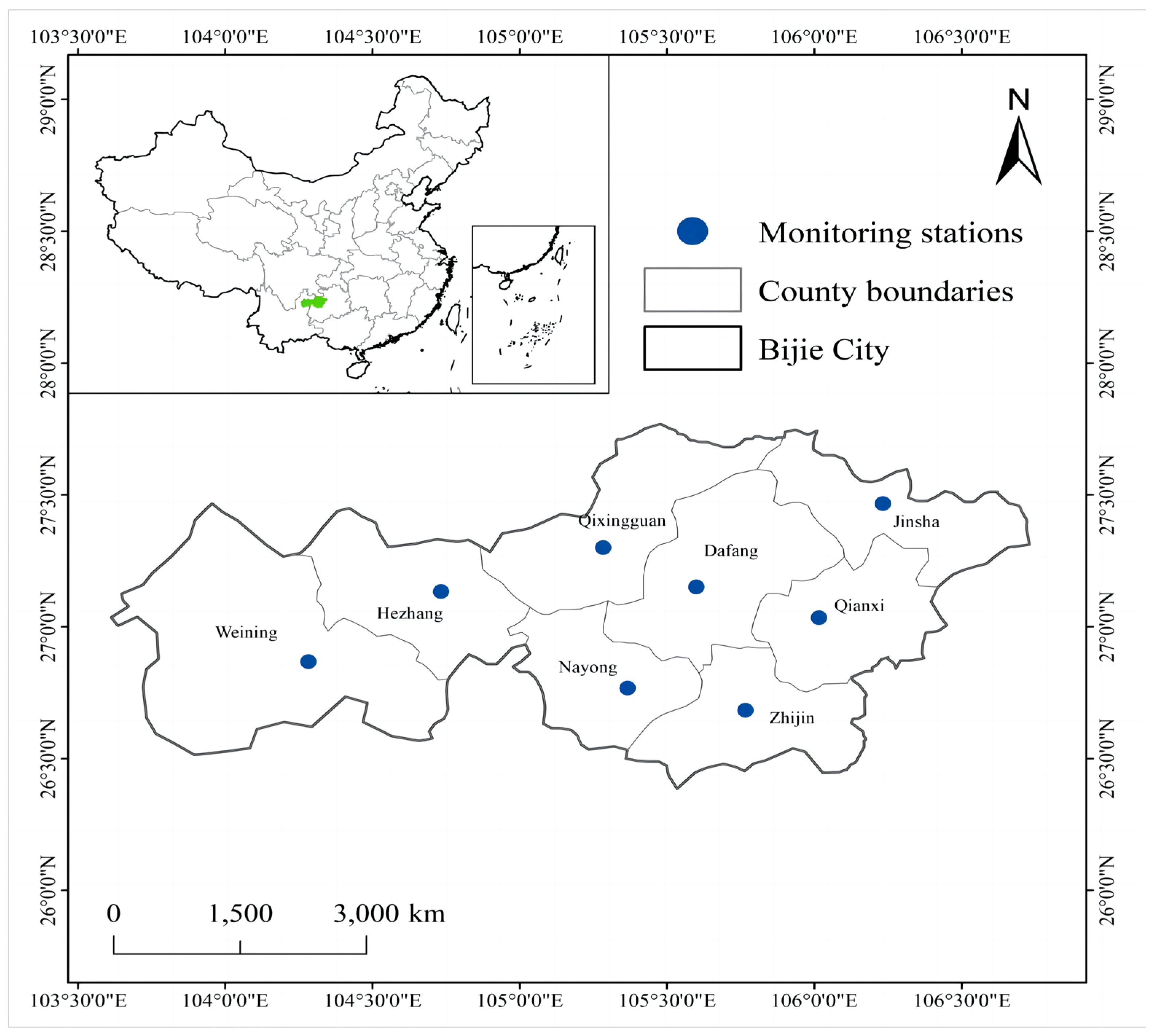
There are eight pollutant monitoring stations in Bijie District; they are located in Qixingguan District, Dafang County, Qianxi County, Jinsha County, Zhijin County, Nayong County, Weining Yi Autonomous County, and Hezhang County. Each region has a monitoring station, so the average data of the eight regional monitoring stations were selected as the experimental data. The study area and site distribution are shown in Figure 1.

The data covers the period from 1 January 2015 to 31 December 2022. The data used are from the National Meteorological Administration, and the observed meteorological variables were provided by eight district and county weather stations. The data samples are hourly meteorological observation results. Each sample contains 14 characteristic elements, including speed, temperature, pressure, precipitation, relative humidity, wind speed, wind direction, precipitation, dew point temperature, and visibility. The environmental monitoring station provides six basic pollutant variables, namely, PM_2.5, PM₁₀, NO₂, SO₂, O₃, CO, and air quality AQI (

Table 1. Variable description.

Data Type	Variables	Unit	Time Resolution
Air pollutants	PM2.5	μg/m3	1 h
	PM10	μg/m3
	SO2	μg/m3
	NO2	μg/m3
	O3	μg/m3
	CO	μg/m3
	AQI	μg/m3
Meteorological observations	Temperature	K	1 h
	Wind speed	m/s
	Wind direction
	Relative humidity	%
	Dew point temperature	K
	Pressure	hPa
	Precipitation	mm
	Visibility	km

).

2.1. Convolutional Neural Network (CNN)

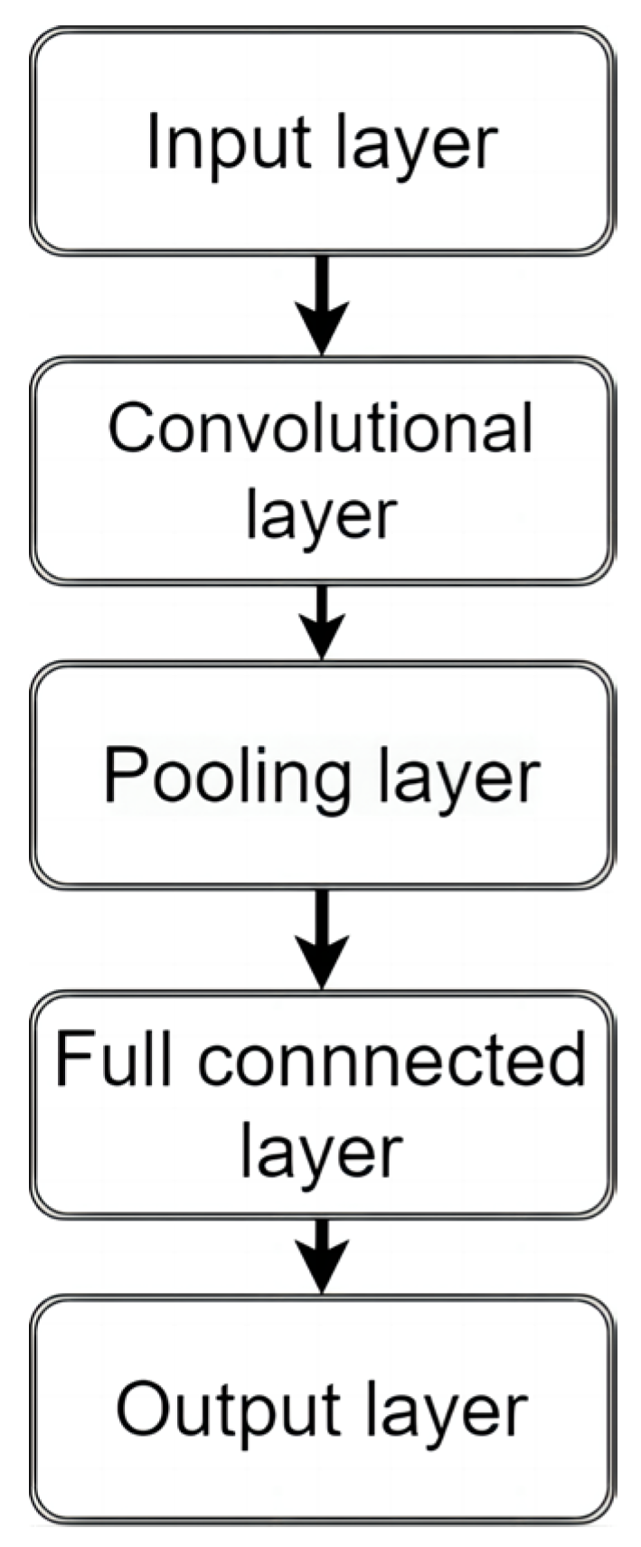
In order to better recognize and make better use of existing features, this study uses a CNN to extract features. A CNN can extract the overall characteristics of data within a certain range from the input data through local perception, weight sharing, and pooled sampling, and is able to eliminate redundant data through pooled sampling as the input of the subsequent model. This greatly improves the data recognition effect of subsequent models. The convolutional layer has the ability to extract features from multiple hidden layers and can share the convolution core. The CNN can easily handle multidimensional data [39]. The convolutional neural network structure is shown in Figure 2.

The input layer is used to obtain input data.

The convolutional layer is used for the convolution of input layer data. The so-called convolution is the inner product of the original data and the intermediate filter matrix to obtain a new characteristic matrix, as shown in Figure 3.

The corresponding formula is as follows:

$$H=f(Lh+R)$$

(1)

where $H$ is the convolution output, $f$ is the activation function, $R$ is the inductive bias, $L$ is the convolution kernel, and $H$ is the input representing the inner product.

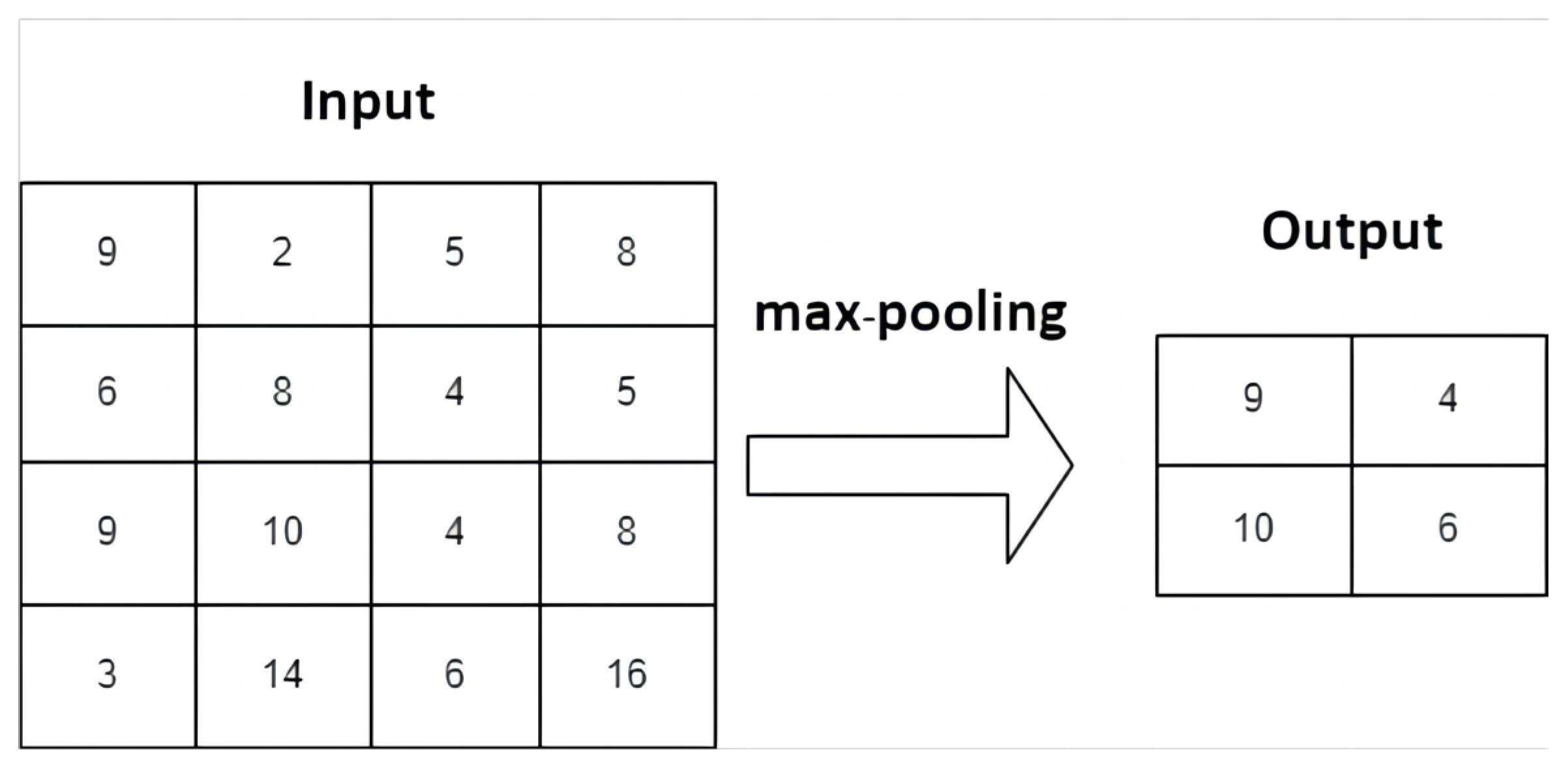
The pooling layer is used to optimize the output of the convolutional layer, reduce the feature dimensions and improve the calculation speed. The pooled data have certain translation and rotation invariance, as shown in Figure 4.

The full connection layer maps all pooled data to the sample tag space for the later output layer.

This paper uses a CNN to extract the features of the input data, and then uses DBiLSTM to predict the data.

2.2. Deep Bidirectional Long Short-Term Memory (DBi-LSTM)

2.2.1. BiLSTM

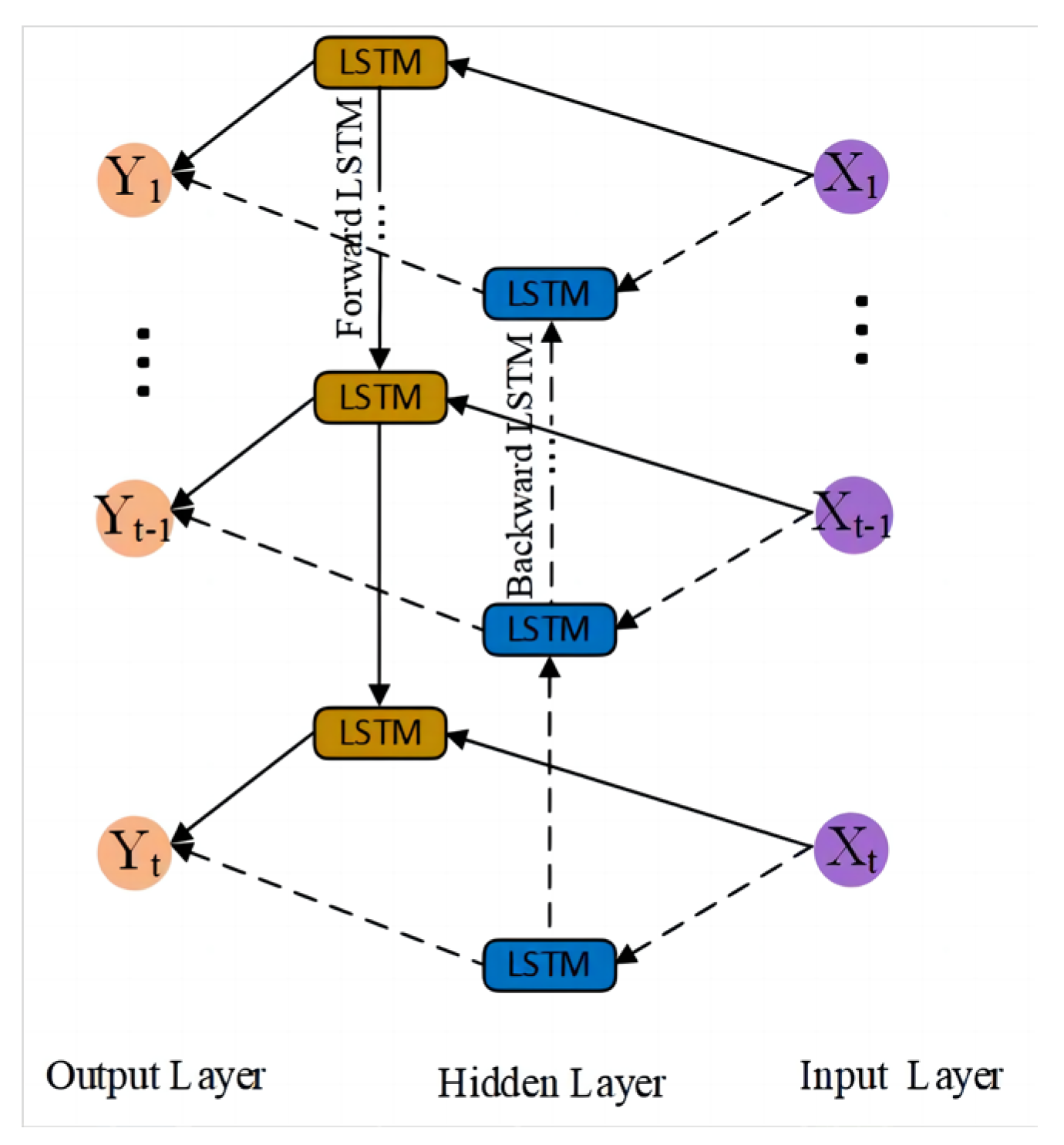
The bi-directional long short-term memory network (BILSTM) is a time-based two-way cyclic network that is trained through the forward time series and the reverse time series. The output data contains information on the entire time series [40]. The BILSTM network is a kind of neural network that is proposed to solve the problem because the long short-term memory network (LSTM) lacks the connection between the front and back data. In essence, the BILSTM network and LSTM network belong to the RNN.

However, the LSTM network can only use the input information from before a certain time to predict the results, so the introduction of the BiLSTM network will produce better results [41]. The two LSTMs are interconnected in the input sequence of the BiLSTM network, such that the information can be used simultaneously in both forward and reverse directions via the present time node’s output. Each time the node’s input is sent in turn to the forward and reverse LSTM units, depending on each of their individual states, they produce outputs. These two outputs are together connected to the output node of the model order, to synthesize the final output. The BILSTM network structure is shown in Figure 5.

2.2.2. DBi-LSTM

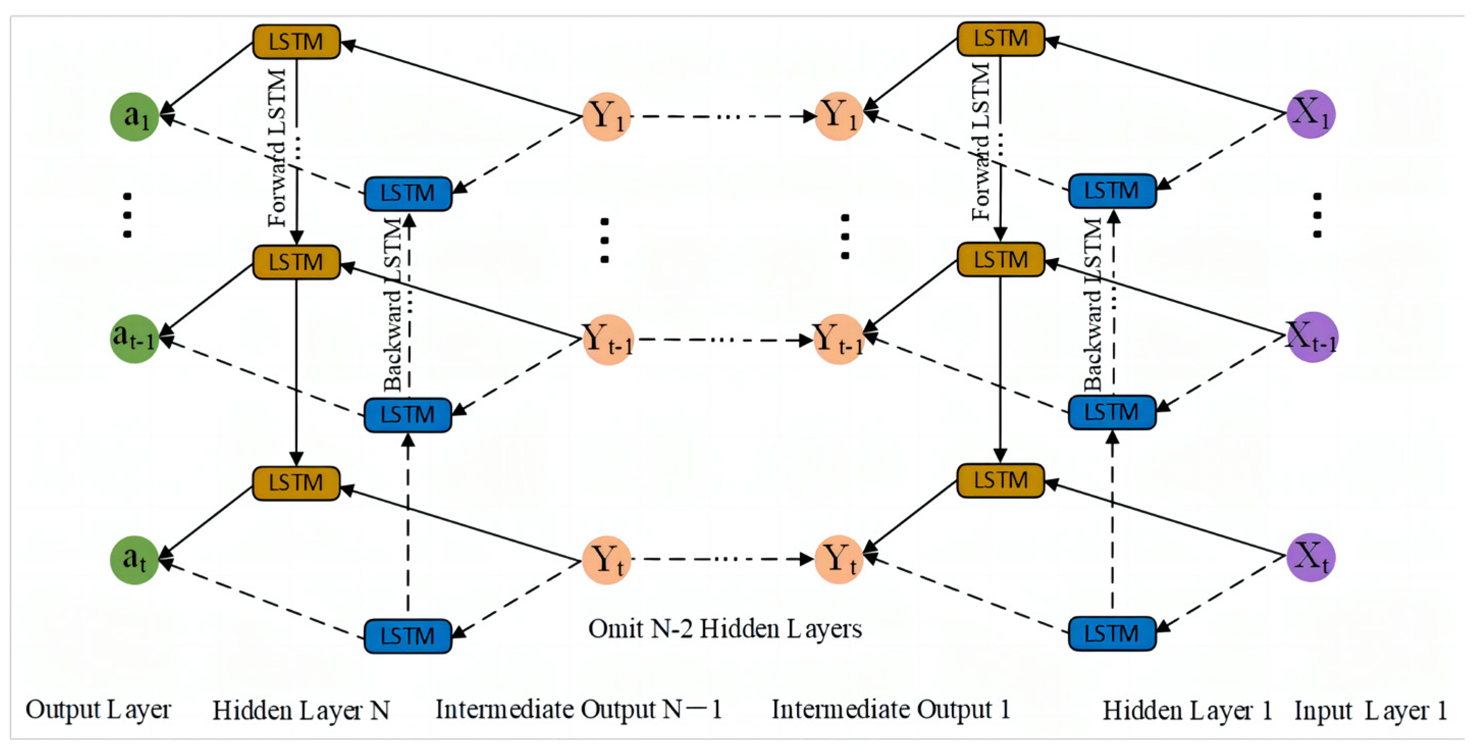
The DBILSTM network is composed of an input layer, an output layer, a hidden layer, and a dense layer. The hidden layer is composed of n BILSTM networks. Each BILSTM layer contains one forward LSTM network and one reverse LSTM network; this enables the BILSTM network at each layer to obtain information from both directions at the same time. The first n − 1, layer will return all output sequences, and then these sequences will be transmitted to the next layer after information fusion through the adder. The nth layer only returns the result of the last time step of the output sequence and outputs the prediction result through the one dense layer (Figure 6). The calculation process is as follows.

Suppose the $\mathrm{i}$th sequence of the DBiLSTM network input is x_i = [x₁, x₂, …x_n, x_m]; then, the output of the first layer can be expressed as

$$H_n^1=f\left(x_i,\overrightarrow{M},\overleftarrow{M}\right)=\left[h_1^1{h}_2^1{h}_3^1{\cdots h}_m^1\right]$$

(2)

where f is the activation function of the BILSTM network; $\overrightarrow{M} \mathrm{a}\mathrm{n}\mathrm{d} \overleftarrow{M}$ are forward and reverse weight matrices, respectively; and $h_n^1={\overrightarrow{h}}_n^1$⊕${\overleftarrow{h}}_n^1$, where superscript 1 indicates the first layer, and ⊕ is the addition calculation. The output sequence of layer v can be expressed as

$$H_n^v=f\left[\left(x_1^{v-1},x_2^{v-1}{x}_3^{v-1}\cdots x_m^{v-1}\right),\overrightarrow{M},\overleftarrow{M}\right]=h_m^V=\left({\overrightarrow{h}}_m^v{\overleftarrow{,h}}_m^v\right)$$

(3)

The final output sequence can be expressed as

$$\left\{\begin{array}{c}{o}_d=g\left(W_d{h}_m^v+b_d\right)\\ y_i=W_O{O}_d\end{array}\right.$$

(4)

where $g$() is the activation function of the dense layer, usually a rule function;$W_O \mathrm{a}\mathrm{n}\mathrm{d} W_d$ are the weight parameters of the dense layer and the output layer, respectively [42]; and $b_d$ is the offset of the dense layer.

2.3. Attention Mechanism

An attention mechanism is a special structure embedded in a machine-learning model and has a large number of applications in many fields. Its essence is that a reasonable distribution model reduces or ignores irrelevant information about the target information and enlarges the important information needed [43]. The attention mechanism mainly causes the model to assign different weight parameters to the input feature vectors in order to adjust the proportion of the input features, highlight the important influence feature vectors, suppress the useless feature vectors, optimize model learning, and make better choices, while not increasing the calculation amount of the model. The structure is shown in Figure 7.

2.4. Sparrow Search Algorithm (SSA)

A novel swarm intelligence optimization algorithm called the SSA was created by modeling the behavior of sparrows seeking food and avoiding predators. Discoverer, enrollee, and watcher are the three categories. The discoverer has a broad search area and can direct the populace toward food. The enrollee will approach the discoverer in order to find nourishment and to become more adaptable. When natural enemies pose a threat to the entire community, the watcher will take off and immediately engage in anti-predation. In general, 10% to 20% of the population are known discoverers. The following is the location update formula:

$$x_{id}^{i+1}=\left\{\begin{array}{c}{x}_{id}^t·exp\left(\frac{-i}{\alpha ·T}\right),R_2\ge ST\\ x_{id}^t+Q·L,R_2\ge ST\end{array}\right.$$

(5)

where $t$ denotes the current iteration count. The maximum amount of iterations is T, Q is a random integer that follows the ordinary normal distribution, and $\mathsf{\alpha }$ is a uniform random number within (0,1) [44]. L means the size is 1 × d in a matrix with all elements of 1;

If $R_2$ < ST, the warning threshold is not reached. When $R_2\ge$ ST, it reaches the threshold of the warning value.

The remaining sparrows, except the discoverers, are all enrollees. They use the following formula to update their positions:

$$x_{id}^{i+1}=\left\{\begin{array}{c}Q·exp\left(\frac{{xw}_d^t-x_{id}^t}{i^2}\right),i>\frac{n}{2}\\ {xb}_d^{t+1}+\frac{1}{D}{\displaystyle \sum _{d=1}^D}\left(rand\left\{-\mathrm{1,1}\right\}·\left|x_{id}^t-{xb}_d^{t+1}\right|\right),i\le \frac{n}{2}\end{array}\right.$$

(6)

$\mathrm{w}\mathrm{h}\mathrm{e}\mathrm{r}\mathrm{e} {xw}_d^t$ stands for the sparrow’s worst position in the d dimension at population iteration t, and ${xb}_d^{t+1}$ stands for the sparrow’s best position in the d dimension at population iteration $t+1$ [45]. If $i>\frac{n}{2}$, the $i$ th person has a low level of fitness. The $i$ th participant has a reasonably high level of fitness when $i\le \frac{n}{2}$. Between 10% and 20% of the population are typically used for reconnaissance and early warning, and their locations are updated as follows:

$$x_{id}^{t+1}=\left\{\begin{array}{c}{xb}_d^t+\beta \left(x_{id}^t-{xb}_d^t\right),f_i\ne f_g\\ x_{id}^t+K\left(\frac{x_{ab}^t-{xw}_d^t}{\left|f_i-f_w\right|+e}\right),f_i=f_g\end{array}\right.$$

(7)

where K is a random number between −1 and 1; $\beta$ is a random number produced by a normal distribution with a mean value of 0 and a variance of 1; $f_i$ is the fitness of the $\mathit{i}$th sparrow; $f_g \mathrm{a}\mathrm{n}\mathrm{d} f_w$ are the best and worst fitness values of the current sparrow population [46]; and $e$ is a very small number to avoid the position being frozen when the denominator is 0.

2.5. CNN-SSA-DBiLSTM-Attention Model

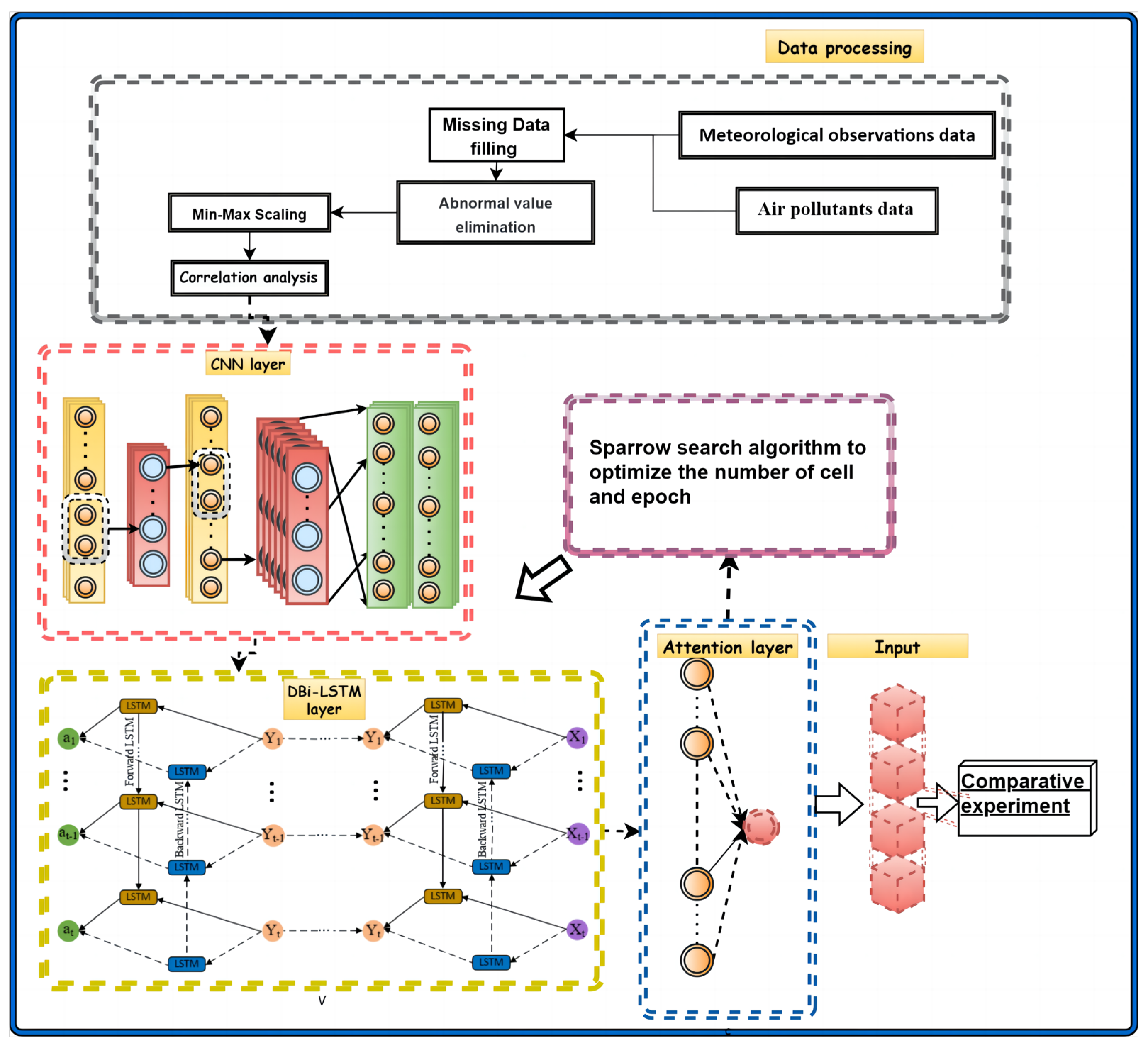
First, a deep bidirectional short-term memory network was established. On the basis of LSTM, the reverse LSTM layer was added, and the bi-directional long short-term memory (BiLSTM) was established. The deep bi-directional long short-term memory (DBiLSTM) was formed by using a multi-layered BiLSTM. Then, a convolutional neural network (CNN) consisting of two convolutional layers, two pooling layers, and two fully connected layers was established to improve the utilization of the feature data. The introduction of an attention mechanism, by mapping weights and learning parameter matrices, reveals the hidden states of different DBILSTM weights to capture important features of long time-series data and enhance the impact of key information. Aiming at the problem of local optimization in the selection of model network parameters, the sparrow search algorithm was used to train the model parameters, improve the prediction accuracy of the model, and finally output the prediction results. The whole process and model structure were as follows (Figure 8):

In this experiment, four evaluation indicators, root mean square error (RMSE), mean absolute error (MAE), mean absolute percentage error (MAPE), and the coefficient of determination (R²), were used to evaluate the model prediction results. The coefficient of determination reflects the level of fitting, the average absolute error reflects the magnitude of the model error, the average absolute percentage error clearly shows the size of the error, and the root mean square error reflects the global stability of the mistake in the model. The formulas are as follows:

$$\mathit{RMSE}=\sqrt{\frac{1}{n}{\sum }_{i=1}^n{\left(y_i-\widetilde{y_i}\right)}^2}$$

(8)

$$\mathit{MAE}=\frac{1}{n}{\sum }_{i=1}^n\left|y_i-\widetilde{y_i}\right|$$

(9)

$$\mathit{MAPE}=\frac{100\mathrm{\%}}{n}{\sum }_{i=1}^n\left|\frac{y_i-\widetilde{y_i}}{\frac{1}{n}{\sum }_{i=1}^n\widetilde{y_i}}\right|$$

(10)

$$R^2 =1-\frac{{\sum }_{\mathit{i}=1}^{\mathit{n}}{\left({\mathit{y}}_{\mathit{i}}-\widetilde{{\mathit{y}}_{\mathit{i}}}\right)}^2}{\mathbf{n}{\sum }_{\mathit{i}=1}^{\mathit{n}}{\left({\mathit{y}}_{\mathit{i}}-\stackrel{-}{{\mathit{y}}_{\mathit{i}}}\right)}^2}$$

(11)

where $y_i$ is the ith predicted value and the ith true value of $\widetilde{y_i}$; n is the total number of data in the test set and $\stackrel{-}{y_i}$ is the average of the true values.

2.6. Data Preprocessing

Missing Value Processing

This study used data from eight stations in Bijie City, with a resolution of 1 h, from 1 January 2015 to 31 December 2022. Owing to the length of time, damage to the sensor itself, or the impact of the environment, there are often data missing and abnormal values in the dataset. In order to improve the accuracy of the model, data cleaning is required. The number of missing air pollutant data and meteorological observation data are shown in

Table 2. Missing data.

Data Type	Variables	Data Missing	Time Resolution
Air pollutants	PM2.5	2%	1 h
	PM10	3.3%
	SO2	1.8%
	NO2	1.3%
	O3	1.6%
	CO	1.3%
	AQI	2.6%
Meteorological observations	Temperature	2%	1 h
	Wind speed	4%
	Wind direction	2.7%
	Relative humidity	3%
	Dew point temperature	3%
	Pressure	3%
	Precipitation	2.3%
	Visibility	9%

. For missing data, this paper used multiple interpolation methods to fill in the data; the mice package in the R language was used to perform the multiple interpolation data filling.

It can be seen from the table that the meteorological data loss is more serious. This is because, in addition to computer failure and monitoring software failure, sometimes the collector, sensor, and other measuring and reporting instruments are hit by lightning when thundery weather occurs. This inevitably leads to instrument damage and failure, resulting in the lack of measurements for all surface meteorological observation data. At the same time, because of the interference of certain complex weather events, the instrument’s collection and transmission of meteorological elements can be affected, resulting in the occurrence of data anomalies. For example, when a rainstorm occurs, the filter covers the temperature and humidity sensor, and the ground temperature sensor is likely to be soaked with rain, resulting in abnormal phenomena, such as missing measurements of temperature and humidity data.

Owing to the influence of different units, the data scale of each influencing factor may vary greatly. In order to make each influencing factor comparable, we need to normalize them. Moreover, for LSTM prediction, the value after the activation function is between −1 and 1, so the data must be normalized. If the data are not normalized, the training speed of the model will slow down, and the final prediction result will be adversely affected.

2.7. Correlation Analysis

For the influencing factors that were initially screened according to experience, we used the collected data to analyze the correlation between the relevant influencing factors and the load.

The correlation between the explanatory variable and the dependent variable (PM_2.5) was calculated, and the correlation coefficient heat plot is shown in

Table 3. Correlation coefficient between various factors and PM_2.5.

Data Type	Variables	Correlation Coefficient
PM2.5	PM2.5	1
	PM10	0.95
	SO2	0.45
	NO2	0.53
	O3	−0.06
	CO	0.36
	AQI	0.92
PM2.5	Temperature	−0.16
	Wind speed	−0.09
	Wind direction	−0.07
	Relative humidity	−0.09
	Dew point temperature	−0.26
	Pressure	0.01
	Precipitation	−0.17
	Visibility	−0.49

. The correlation analysis shows that PM_2.5 has a large positive correlation with PM₁₀ and the air quality index, and the correlation coefficients with PM₁₀ and the air quality index are 0.95 and 0.92, respectively, illustrating the importance of PM₁₀ and AQI as input variables. Following PM₁₀ and AQI, the order of correlation coefficients is NO₂, SO₂, and CO. The correlation between NO₂ and PM_2.5 is 0.53. The correlation between SO₂ and PM_2.5 is 0.48. The correlation between CO and PM_2.5 is 0.36. However, O₃ is also an environmental pollutant, and it has a weak negative correlation with PM_2.5. This is because the main source of PM_2.5 is anthropogenic emissions, such as the combustion of fossil fuels and the emission of automobile exhaust, and the NO₂, SO₂, and CO contained in these emissions generate PM_2.5 through a variety of chemical and physical processes in the atmosphere. PM_2.5 is one of the variables used to calculate the air quality index. O₃ in the near-surface (troposphere) atmosphere is mainly produced by a photochemical reaction, which is different from the source and mode generation of PM_2.5.

In the meteorological data, there is a strong negative correlation between visibility and PM_2.5. The correlation coefficient is −0.49, indicating that visibility decreases when the concentration of PM_2.5 increases. The negative correlation with dew point temperature is second only to visibility, and the correlation coefficient is −0.26, which indicates that the dew point temperature has a good correlation with PM_2.5. Other meteorological data, including wind direction, temperature, precision, relative humidity, and wind speed, are also negatively correlated. It can also be seen from Table 3 that the correlation between other variables and PM_2.5 is not high, and the correlation coefficient between pressure and PM_2.5 is only 0.01, indicating that there is almost no relationship between pressure and PM_2.5. In order to improve the prediction accuracy, we removed pressure, which had the lowest correlation coefficient in order, to reduce the data dimensions.

3. Results and Discussions

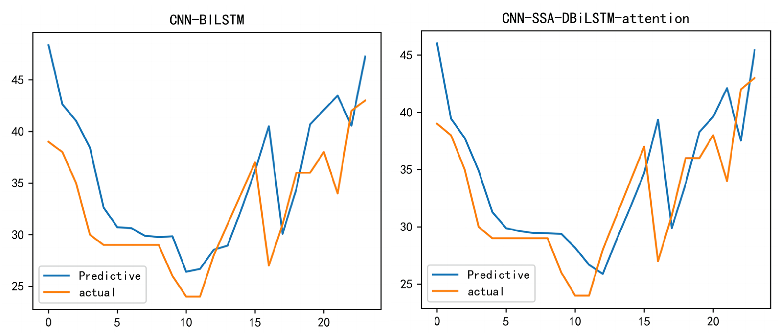
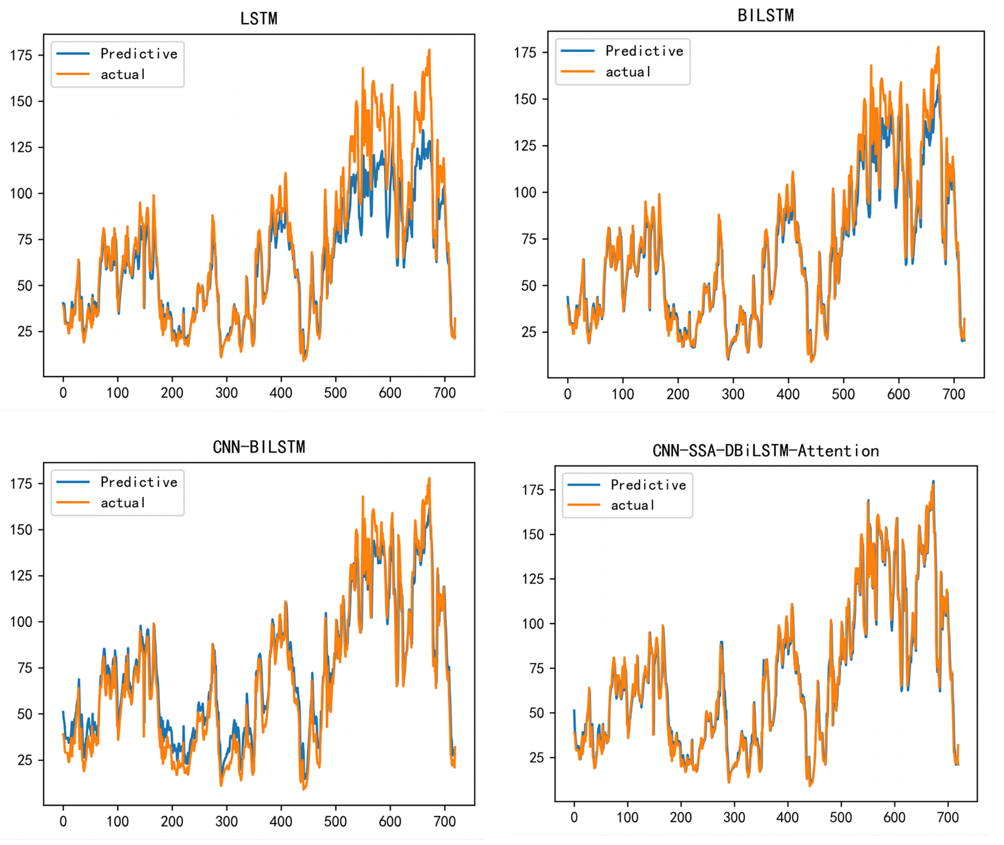
In order to study the visible prediction performance of the proposed hybrid model, the prediction results of Bijie City after 24 h, 48 h, 168 h, and 720 h were analyzed using a CNN-SSA-BILSTM-attention model and compared with three basic models, CNN-BILSTM-attention, LSTM, and BILSTM. CNN-SSA-BILSTM-attention shows good prediction results at 24 h, 72 h, 168 h, and 720 h. We forecasted and compared the 2021 winter data. The reason we used the winter data from 2021 was that PM_2.5 fluctuated greatly during this period, and the difference between the lowest concentration value and the highest concentration value exceeded 60—this requires a model with a high prediction accuracy.

According to the short-term prediction results for 24 h and 72 h, CNN-SSA-DBiLSTM-attention shows good prediction performance in the short-term PM_2.5 prediction. In the 24 h prediction, the coefficient of the determination (R²) of CNN-SSA-DBiLSTM-attention is 0.95, which is higher than the 0.92 and 0.89 of CNN-BiLSTM and LSTM. It is far higher than the 0.82 of LSTM. With regard to the three parameters of the root mean square error (RMSE), mean absolute percentage error (MAPE), and mean absolute error (MAE), the effects of the CNN-SSA-DBiLSTM-attention models are also better than other three models. From Figure 9, it can be seen that CNN-SSA-DBiLSTM-attention has the best prediction performance. Compared to other models, the predicted values are more in line with the actual values. The worst result in the graph is BILSTM. 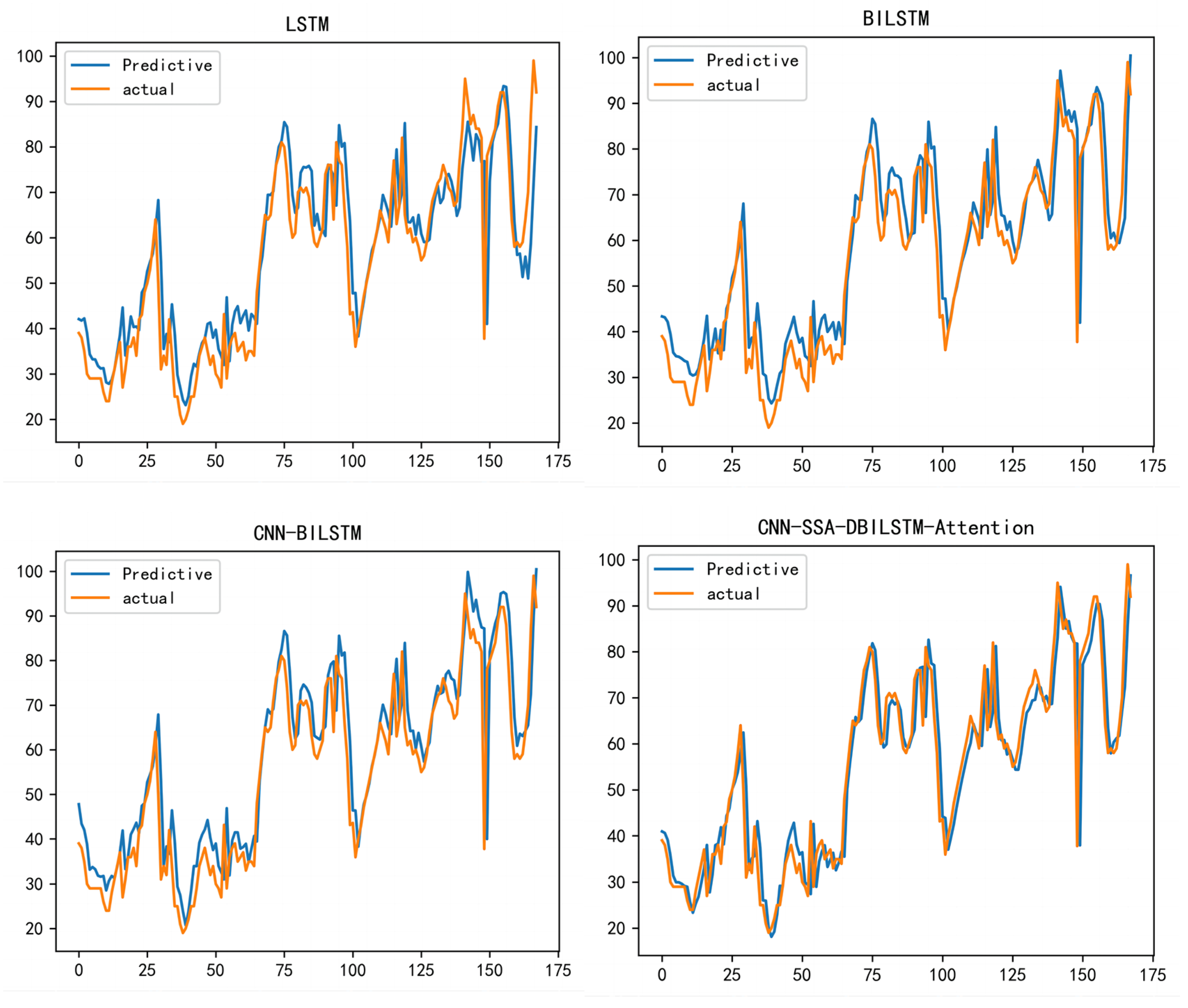For the 72 h forecast, the evaluation values of the CNN-SSA-DBiLSTM-attention model are: RMSE 10.29, MAPE 9.44, MAE 6.41, and R² 0.94. These are the four models that have the best neutral energy. Additionally, the LSTM with the worst performance has evaluation values of RMSE 18.95, MAPE 14.80, MAE 11.24, and R² 0.82. From Figure 10, it can be seen that the consistency between the true and predicted values of the CNN-SSA-DBILSTM-attention model is much higher than that of the other three models. The predicted values of the CNN-SSA-DBiLSTM-attention model are basically consistent with the trend of the actual values. The overall accuracy of the CNN-SSA-DBiLSTM-attention model proposed in this paper is higher, from the perspective of 24 h and 72 h prediction (

Table 4. PM_2.5 prediction (24/72 h) results. The left values are the 24 h data and the right values are the 72 h data.

Model	RMSE 24 h/72 h	MAPE 24 h/72 h	MAE 24 h/72 h	R2 24 h/72 h
CNN-SSA-DBiLSTM-attention	10.10/10.29	9.39/9.44	6.27/6.41	0.95/0.94
CNN-BILSTM	12.12/5.12	10.26/12.87	7.30/3.06	0.92/0.93
BILSTM	14.49/15.59	13.01/11.98	9.42/8.96	0.89/0.88
LSTM	18.95/18.90	15.49/14.80	11.91/11.24	0.82/0.82

and

Table 5. PM_2.5 prediction (168 h/720 h) results. The left shows 168 h data and the right shows 720 h data.

Model	RMSE 168 h/720 h	MAPE 168 h/720 h	MAE 168 h/720 h	R2 168 h/720 h
CNN-SSA-DBiLSTM-attention	9.05/10.14	10.28/9.68	5.78/6.22	0.96/0.95
CNN-BILSTM	11.96/12.59	12.45/13.35	7.42/9.30	0.92/0.92
BILSTM	13.74/14.04	12.45/12.49	8.95/8.92	0.91/0.90
LSTM	18.62/16.53	14.74/13.19	11.32/10.96	0.83/0.86

).

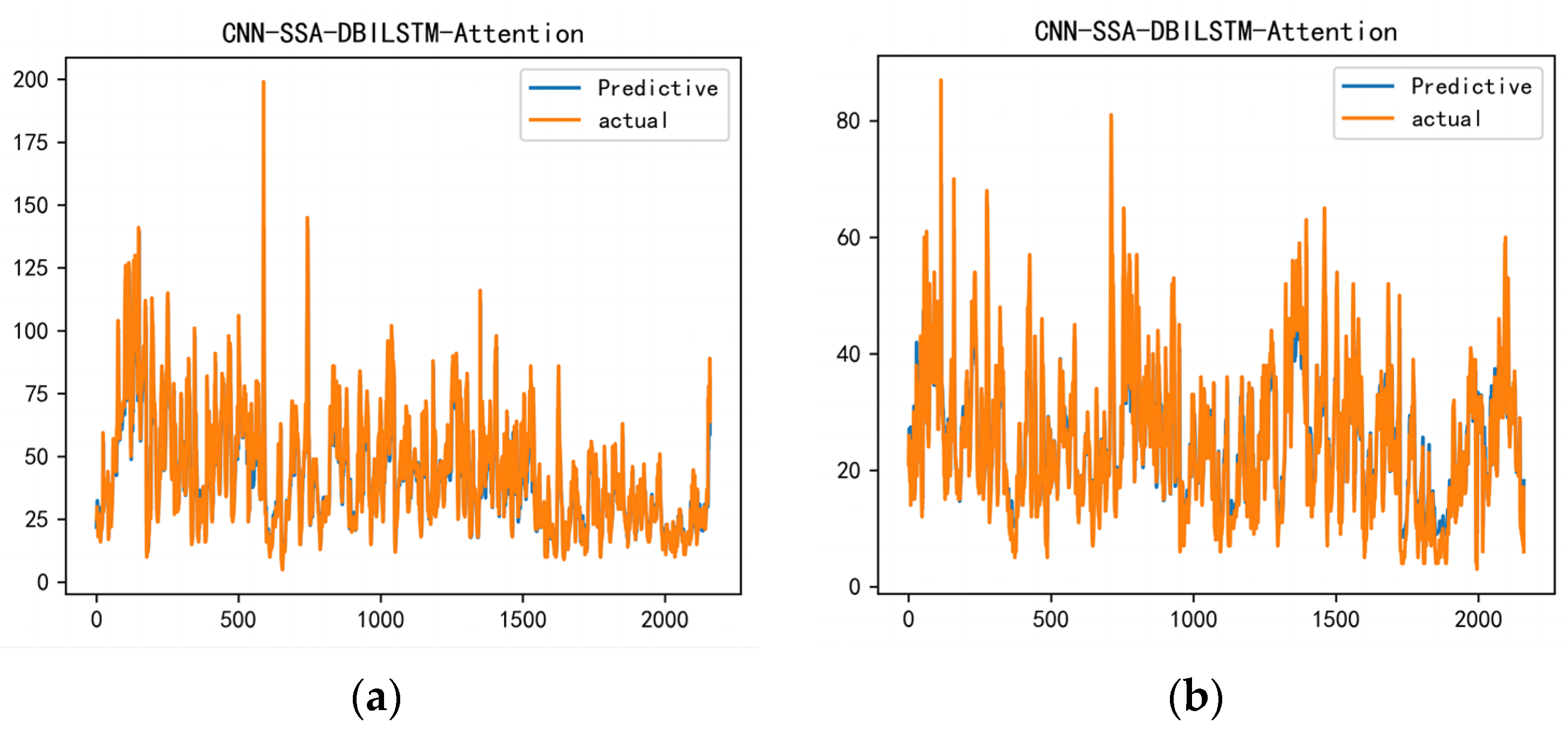
According to the short-term prediction results for a week and a month, in terms of PM_2.5 prediction, the accuracy of the CNN-SSA-DBiLSTM-attention model proposed in this paper is significantly higher than that of the other three comparison models: RMSE 9.05/10.14, MAPE 10.28/9.68, MAE 5.78/6.22, and R² 0.96/0.95. Each evaluation value is superior to the other three models. From the comparison between the real value and the predicted value, when the time span is one week, the curves of the predicted value and the real value are basically the same. The degree of coincidence is also quite close. When the time span is one month, the curves of the predicted value and the real value are basically the same, and the coincidence degree is almost total. Overall, the model proposed in this article exhibits good predictive performance at 24 h, 72 h, 168 h, and 720 h. The R² stability of the CNN-SSA-DBiLSTM-attention model at 0.95 is much better than the other three models. CNN-SSA-DBiLSTM-attention model’s MAPE, RMES, and MAE values are also better than those of the other three models. Overall, the LSTM model has the worst performance. CNN-BILSTM and BILSTM have good performance. The CNN-SSA-DBiLSTM-attention model performs 15% better than the LSTM model. It can also be seen from the chart that the degree of coincidence between the predicted value curve and the true value curve increases significantly with the increase in time. This reflects the excellent performance of the model in short-term prediction that is proposed in this article (Figure 11 and Figure 12).

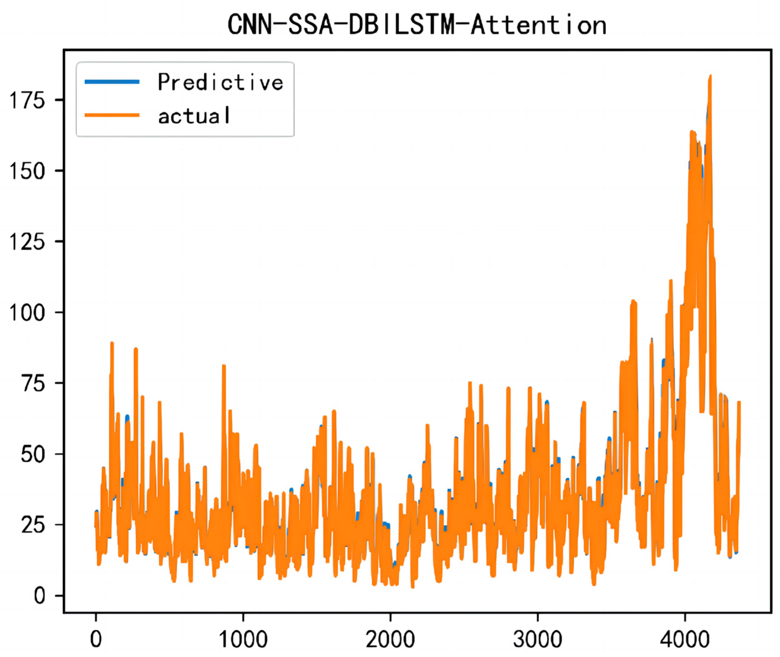
In order to better verify the accuracy of the model for long-time-span prediction, this paper used the CNN-SSA-DBiLSTM-attention model to predict PM_2.5 concentration after half a year. The prediction results are shown in Figure 13. It can be seen from the figure that the predicted value and true value almost completely fit; RMSE is 6.20, MAPE is 11.93, MAE is 4.08, and R² is 0.96. Compared with the short-term PM_2.5 prediction results, the prediction accuracy of PM_2.5 over a time span of six months remains stable. The coefficient of determination is 0.96. This indicates that the model proposed in this article has better prediction accuracy for long-term span prediction.

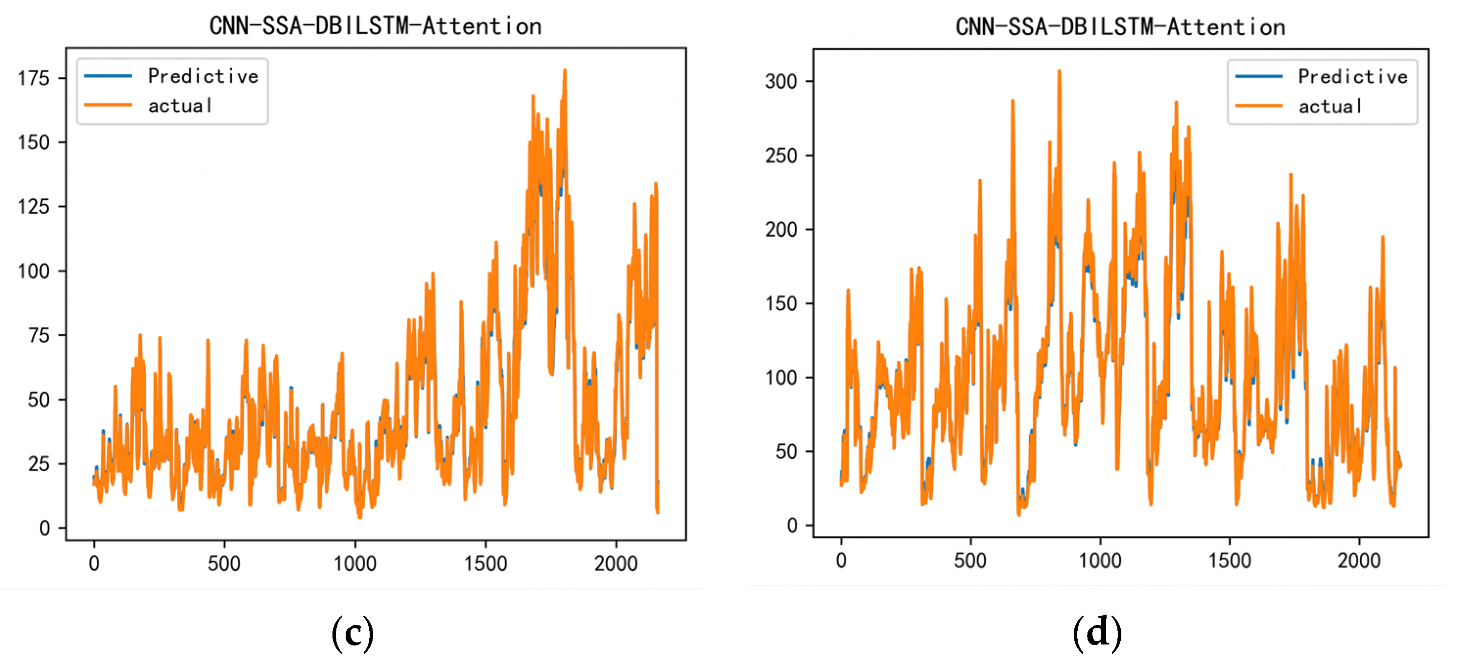
It is beneficial to study the applicability of the model in different seasons and the impact of different seasons on the model’s accuracy. This paper also forecasted and analyzed data from the four seasons, namely spring, summer, autumn, and winter. The results are shown in

Table 6. PM_2.5 prediction (spring, summer, autumn, and winter) results.

	Model	RMSE	MAPE	MAE	R2
Spring	CNN-SSA-DBiLSTM-attention	5.25	12.29	3.42	0.94
	CNN-DBILSTM	5.83	12.64	4.45	0.91
	BILSTM	5.86	15.94	4.62	0.90
	LSTM	8.87	13.12	5.48	0.84
S ummer	CNN-SSA-DBiLSTM-attention	3.92	10.13	4.03	0.95
	CNN-DBILSTM	5.28	14.44	4.47	0.92
	BILSTM	5.99	14.76	6.36	0.88
	LSTM	7.91	15.41	7.70	0.85
A utumn	CNN-SSA-DBiLSTM-attention	7.64	12.10	4.63	0.95
	CNN-DBILSTM	8.49	13.25	5.46	0.92
	BILSTM	9.96	15.94	6.76	0.90
	LSTM	10.07	15.45	8.13	0.85
Winter	CNN-SSA-DBiLSTM-attention	8.87	9.89	6.58	0.96
	CNN-DBILSTM	11.96	10.42	9.42	0.93
	BILSTM	14.42	11.74	9.78	0.89
	LSTM	17.32	13.19	10.11	0.85

. According to the results in the table, the model proposed in this paper is better than the other three models, in terms of R², MAPE, RMSE, and MAE values, in spring, summer, autumn, and winter. In spring, RMSE is 5.247, MAPE is 12.288, MAE is 3.424, and R² is 0.94. In summer, RMSE is 3.902, MAPE is 10.128, MAE is 4.033, and R² is 0.95. In autumn, RMSE is 7.642, MAPE is 12.096, MAE is 4.629, and R² is 0.95. In winter, RMSE is 8.871, MAPE is 9.890, MAE is 6.579, and R² is 0.96. The prediction results are shown in Figure 14.

4. Conclusions

Based on the hourly air quality historical data and meteorological dataset of Bijie City from 1 January 2015 to 31 December 2022, this paper conducted empirical research and drew the following conclusions:

From the chart in the text, it can be seen that there are multiple cases of PM_2.5 exceeding 100. This indicates that the atmospheric conditions in the Bijie area are poor. The correlation analysis results show that PM₁₀ is the most important input variable, followed by the air quality index. The correlation coefficients of PM₁₀ and the air quality index with PM_2.5 are 0.95 and 0.92, respectively, and they have an important impact on PM_2.5. NO₂, SO₂, CO, and other factors that also have an impact on PM_2.5. O₃ has a negative correlation with PM_2.5 and has an inhibiting effect on PM_2.5. Temperature, rainfall, wind speed, and humidity also have an inhibiting effect on PM_2.5. The most important meteorological factor is visibility, and it has a strong negative correlation with PM_2.5. Precipitation and dew point temperature are also relatively important variables. Overall, meteorological factors have little impact on PM_2.5. Four models were used to predict PM_2.5 concentration. The results showed that the prediction accuracy of the CNN-SSA-DBiLSTM-attention model is the highest, and the coefficient of determination was stable at about 0.95. In contrast, the prediction accuracy of the LSTM model is poor, and the coefficient of determination is 0.84. The overall performance of the CNN-BILSTM and BILSTM models are not as good as those of the CNN-SSA-DBiLSTM attention model. However that model also achieve good prediction results. Surprisingly, the model proposed in this article has high accuracy in both short-term and long-term predictions. Additionally, it also maintains high accuracy in predicting different seasons and was not affected by seasonal changes. In the PM_2.5 prediction model, it can be seen that the values of rems and map will fluctuate due to the different seasons. This is due to different concentrations of PM_2.5 during different seasons. This indicates the effectiveness of the proposed model and indicates that the hybrid model is able to effectively improve prediction accuracy. The use of hybrid models to improve the accuracy of PM_2.5 prediction is a promising research direction. In future research, researchers should make more use of fusion models for prediction and to optimize model structures.