Article

Regional Tropospheric Correction Model from GNSS–Saastamoinen–GPT2w Data for Zhejiang Province

1
School of Geodesy and Geomatics, Wuhan University, Wuhan 430079, China
2
Wenzhou Institute of Geotechnical Investigation, Surveying and Mapping, Wenzhou 325000, China
3
Earth System Science Programme, Faculty of Science, The Chinese University of Hong Kong, Hong Kong 999077, China
4
Chinese Antarctic Center of Surveying and Mapping, Wuhan University, Wuhan 430079, China
5
Zhuhai Surveying and Mapping Institute, Zhuhai 519000, China
*
Author to whom correspondence should be addressed.
Atmosphere 2023, 14(5), 815; https://doi.org/10.3390/atmos14050815
Submission received: 6 April 2023 / Revised: 26 April 2023 / Accepted: 28 April 2023 / Published: 30 April 2023
(This article belongs to the Section Atmospheric Techniques, Instruments, and Modeling)

Abstract

:
Tropospheric delay models based on GNSS observations are essential for studying tropospheric changes. However, the uneven distribution of GNSS stations reduces the accuracy of GNSS tropospheric delay models in remote areas. Moreover, the accuracy of the tropospheric delay calculated by traditional models, which rely on meteorological parameters, is lower compared to the accuracy achieved by GNSS tropospheric models. At present, there are sufficient surface meteorological observation facilities around the world that can obtain surface meteorological parameters in real time. It is of great importance to make full use of the measured meteorological parameters to establish tropospheric correction models. Moreover, the empirical tropospheric models use free and open data, and one can obtain tropospheric parameters through the model without requiring any auxiliary information. We established a provincial real-time regional tropospheric fusion model using ground-based GNSS observations, a meteorological model, and empirical model data. Results showed that the tropospheric delay observations of the three models can be fused to establish a real-time tropospheric delay model with better accuracy and higher spatiotemporal resolution. The accuracy of Zenith Total Delay (ZTD) estimated by the fusion model reached 0.96/1.04/3.11 cm during the tropospheric quiet/active/typhoon period.

1. Introduction

The troposphere is the first layer of the Earth’s atmosphere and contains most of its water vapor. Motion in the troposphere is the cause of most weather and climate events and is, thus, closely related to the daily lives of humans, animals, and plants. In the precision positioning applications of GNSS, the tropospheric delay is one of the main sources of errors [1]. The error caused by tropospheric delay in GNSS can be larger than 2 m. Ignoring the impacts of the tropospheric delay error will introduce large errors to the positioning results, making high-accuracy positioning difficult to achieve. At present, these errors can be considered by one of two methods. The tropospheric delay can be treated as a parameter, the value of which is estimated using a filter or an estimator, or the error is precisely corrected using an appropriate tropospheric model. In GNSS real-time precise positioning applications, the first method often requires a certain filter convergence time [2]. The tropospheric modeling involved in the second method usually contains certain errors as well, which leads to a reduction in the accuracy of real-time positioning results [3,4]. As the use of GNSS expands, users are expected to acquire rapid and stable location services with high accuracy in real-time, which sets increasingly higher requirements for the accuracy of real-time tropospheric models. In general, the commonly used tropospheric delay models are divided into three types: empirical tropospheric models, meteorological tropospheric correction models, and GNSS tropospheric correction models.
In the late 1990s, Collins and Langley proposed a precise empirical model, the University of New Brunswick (UNB) model, which had an accuracy of about 5 cm [5]; later models in this series have been proposed continuously. With the development of the Numerical Weather Model (NWM) product ERA-40 by the European Centre for Medium-range Weather Forecasts (ECMWF), [6] proposed a modified tropospheric projection function, called the Global Mapping Function (GMF) for GNSS and Very Length Baseline Interferometry (VLBI) technologies using a large amount of NWM data. Reference [7] proposed a new tropospheric correction model, the Global Pressure and Temperature (GPT), using ERA-40 data, which Kouba then applied to the analysis of GNSS- and GNSS-related applications [8]. In order to achieve fast convergence in GNSS precise positioning, Lu et al. established a tropospheric modeling method constrained by NWM to improve the precise point positioning of multi-system GNSS, which shortened the convergence times of the E, N, and U components by 20.0, 32.0, and 25%, respectively [9]. Reference [10] produced an improved version of the GPT model mentioned above, called the GPT2 model, which is an empirical model precisely based on 10 years of NWM data and temperature and pressure variations. Reference [11] later improved the GPT2 model, extending it to the GPT2w model. In comparison to the GPT2 model, two additional estimated parameters were added, namely, the rate of water vapor decline and weighted mean atmospheric temperature, and the horizontal resolution of the model was increased to 1° × 1° to provide better accuracy and reliability [11]. Reference [12] further optimized and upgraded the tropospheric mapping function in GPT2w and named the new version GPT3 model. Since the calculation of tropospheric delay in the GPT3 model is the same as that in GPT2w, and the focus of this study is on tropospheric delay, the GPT2w model was used to calculate tropospheric delay in this study. The meteorological tropospheric correction models widely used in GNSS positioning applications were mostly proposed around the 1970s. The Hopfield model proposed in 1969 can provide decimeter-level corrections for the effects of the troposphere on Doppler measurements and ranging observations [13], but its accuracy decreases as the elevation of the station increases [14]. To facilitate the implementation of this model, Black proposed a simplified version of Hopfield’s method in 1978, called the Black method [15]. Based on contemporary model evaluation and analysis [16,17], the Saastamoinen method proposed in 1972 has provided a relatively universal and precise correction for the tropospheric delay [18]. Each method above requires meteorological data from climate monitoring stations, the accuracy of which is at the centimeter scale under optimal performance conditions, and at the decimeter scale overall.
At present, continuously operating reference station(s) (CORS) have been established in many areas. Each GNSS observation data point in CORS is used to calculate the ZTD over the station, after which, the regional modeling is performed, and the model results are broadcast to the users. Tao—in his master’s thesis—used Jet Propulsion Laboratory (JPL) real-time orbits, clock products, and precise point positioning (PPP) technology to establish a near-real-time system for Canada’s geodetic CORS network. The accuracy of the precipitable water vapor (PWV) results in this system reached 2 mm, and the ZTD accuracy reached 13 mm [19]. Ye et al. compared the real-time and post-processing of PPP tropospheric delay estimations and showed that the accuracies of real-time and post-processing were 20 mm and 6 mm, respectively [20]. As the Centre National D’Etudes Spatiales (CNES) began to routinely provide real-time results, enabling the users to use PPP correction services over the internet [21], the CNES results have also been applied in the base stations of the internet to provide the tropospheric service PWV [22]. Shi et al. used real-time PPP to estimate the ZTD of each station in the Wuhan CORS network and then calculated the optimal polynomial model coefficients to determine the local tropospheric model [23]. As described by them, the use of this tropospheric model improved the convergence speed and accuracy of the precise positioning.
In summary, although the various tropospheric delay models that are currently applied globally have their unique advantages and shortcomings, the data types they use are relatively consistent and, thus far, there has been little research into multi-source tropospheric data fusion modeling. The schemes that have been used include different models, such as empirical methods performed by the GNSS network, meteorological models, and large-scale real-time tropospheric observations, which can all achieve precise tropospheric corrections and provide precise positioning results. However, each method has its limitations. We present a real-time tropospheric fusion model for the Zhejiang Province by using multi-source data, including GNSS observation data, meteorological data, and the GPT2w empirical model; moreover, the performance of the model was evaluated.

2. Materials and Methods

2.1. Saastamoinen Model

The tropospheric delay model proposed by Saastamoinen, which is based on meteorological parameters, can calculate the ZTD using the latitude and elevation of the observation station, air temperature, atmospheric pressure, and water vapor pressure. The calculation formula of the Saastamoinen model is shown as follows:
Z T D = 0.0022768 1 0.00266 cos ( 2 φ ) ( P + ( 1255 T ) e )
where P is the atmospheric pressure of the station (hPa), T is the absolute temperature at the station (K), e is the water vapor pressure at the station (hPa), φ is the station’s latitude (Radian), and H is its ground elevation (m).
At present, there is a sufficient number of surface meteorological observation facilities in all areas around the world, which can be used to obtain surface meteorological parameters, such as air temperature, atmospheric pressure, and water vapor pressure in real time. The relevant data can be obtained from the meteorological department or by using self-constructed meteorological observation stations.

2.2. GPT2w Model

The GPT2w model is an empirical tropospheric model established using the meteorological data from ECMWF. The parameters involved include air temperature, atmospheric pressure, air temperature lapse rate, water vapor pressure, mapping function coefficients, weighted mean atmospheric temperature, and the rate of water vapor decline. This model considers the annual and semi-annual periods of the tropospheric parameters simultaneously. The model expression is shown as follows:
a = a 0 + A 1 cos ( d o y 365.25 2 π ) + B 1 sin ( d o y 365.25 2 π ) + A 2 cos ( d o y 365.25 4 π ) + B 2 sin ( d o y 365.25 4 π )
where a is a parameter to be evaluated, a 0 is the mean value, A 1 and B 1 are annual period coefficients, A 2 and B 2 are semi-annual period coefficients, and doy is the day of the year. The GPT2w model uses grids with resolutions of 5° × 5° and 1° × 1° for global expressions, i.e., the global area is divided by the grid to obtain the coefficients for each grid point. When using the model, the estimated parameters at the four grid points around the target station at its specific elevation need to be calculated, and then bilinear interpolation is performed to interpolate the parameter values for the station. After calculating the atmospheric temperature, GPT2w uses the Saastamoinen model to calculate the zenith hydrostatic delay (ZHD), and uses the AN model [24] to calculate the zenith wet delay (ZWD), whose formula is shown as follows:
Z W D = 10 6 ( k 2 + k 3 T m ) R d ( λ + 1 ) g m e s
where k 2 and k 3 are atmospheric refractive index constants, taking the values given by Thayer (1974), where k 2 is 16.529 k· m b 1 and k 3 is 3.776 × 10⁵ k·m b 1 . Tm is the weighted mean atmospheric temperature, g m is the gravitational acceleration, R d is the specific gas constant of dry air with a value of 287.058 J·kg 1 ·K 1 , and es is the water vapor pressure (hPa). λ is calculated as follows:
e e 0 = ( P P 0 ) λ + 1
requiring the fitting of meteorological contour data at the station; it is also one of the meteorological parameters provided by GPT2w.
ZTD is equal to the sum of ZHD and ZWD. Therefore, as an empirical model, GPT2w can provide empirical ZTD values for any time and location.

2.3. Real-Time PPP-Estimated ZTD

Before the IGS RTS can provide the real-time precise orbits and clock correction results, the ZTD is often estimated using the double-difference method. However, this method requires the introduction of GNSS stations from 500 km away. At present, IGS RTS products and the PPP technology can be used to calculate the ZTD of a single GNSS station. The solution for PPP uses ionospheric-free combinations, the functions of which are shown in:
P I F = ρ + T c d t s + c d t r + ε P L I F = ρ + T c d t s + c d t r + λ I F N I F + ε L T = Z W D × m f w + Z H D × m f h
where P I F is the pseudo-range observation of the ionospheric-free combination, ρ is the geometric distance from the satellite to the station, c is the speed of light in vacuum, d t s and d t r are the errors of the satellite and the receiving clock, respectively, ε P is the pseudo-range observation noise of the combination, L I F is the phase observation of the ionospheric-free combination, λ I F and N I F are the phase observation wavelength and ambiguity of the combination, respectively, ε L is the phase observation noise of the combination, T is the effect of the tropospheric delay, and ZWD is a parameter to be evaluated. ZHD is provided by the GPT2w model. m f w and m f h are the mapping functions of the wet and dry troposphere, respectively, and are also provided by the GPT2w model. In the solution for PPP, ZTD can be obtained by summing the estimated ZWD and the ZHD calculated by GPT2w.

2.4. Regional Multi-Source Tropospheric Fusion Modeling

Based on the area of the experimental regions, a quadratic polynomial model was used to express the regional tropospheric fusion model, and three different ZTD data sources are utilized in this paper. The observation equations of the fusion model are shown in Formula (6),
Z T D G N S S i = a 0 + a 1 B i + a 2 L i + a 3 h i + a 4 B i L i + a 5 B i h i + a 6 L i h i + a 7 B i 2 + a 8 L i 2 + a 9 h i 2 Z T D S A j = a 0 + a 1 B j + a 2 L j + a 3 h j + a 4 B j L j + a 5 B j h j + a 6 L j h j + a 7 B j 2 + a 8 L j 2 + a 9 h j 2 + C S A Z T D G P k = a 0 + a 1 B k + a 2 L k + a 3 h k + a 4 B k L k + a 5 B k h k + a 6 L k h k + a 7 B k 2 + a 8 L k 2 + a 9 h k 2 + C G P
where i, j, and k represent the different station numbers. Each data source covered multiple stations. Z T D G N S S i refers to the ZTD observation value from the GNSS station, Z T D S A j is the ZTD calculated by the Saastamoinen model using data from meteorological observation stations, Z T D G P k is the ZTD calculated by the GPT2w model, a 0 a 9 are model coefficients, and L, B, and h are the latitude, longitude, and elevation of the station, respectively. The fusion model uses the ZTD calculated by GNSS as the reference, and C S A is the systematic error of the Saastamoinen model and C G P is the systematic error of the GPT2w model.
The parameters to be solved include ten model coefficients and two systematic errors, leaving twelve parameters in total to be evaluated, which were solved using the least-squares method. In the estimation process, the weightings need to be reasonably determined. Since the accuracies of ZTD from the GNSS, Saastamoinen model, and GPT2w models are inconsistent, the weightings of different types of observation data needed to be considered in the process of fusion of the multi-source data. Prior accuracies of different types of ZTD estimations are set first. The accuracy of the empirical model GPT2w was about 4 cm, the accuracy of the Saastamoinen model was about 3.5 cm, and the accuracy of the GNSS real-time estimation was about 1.5 cm. In order to reasonably determine the weightings of the different types of observations, the Helmert variance component estimation method [25] was applied. However, using the Helmert variance component estimation method directly may cause the weighting of GNSS to be lower than those of the other methods. In fact, the ZTD estimated by GNSS had the best accuracy and stability. Therefore, in the weighting process applied in this study, the initial weightings for various types of observations were set according to their prior accuracies. Then the Helmert variance component estimation method was applied to determine the weightings on the basis that the GNSS observations maintained the largest weighting.

2.5. Introduction of Experimental Data

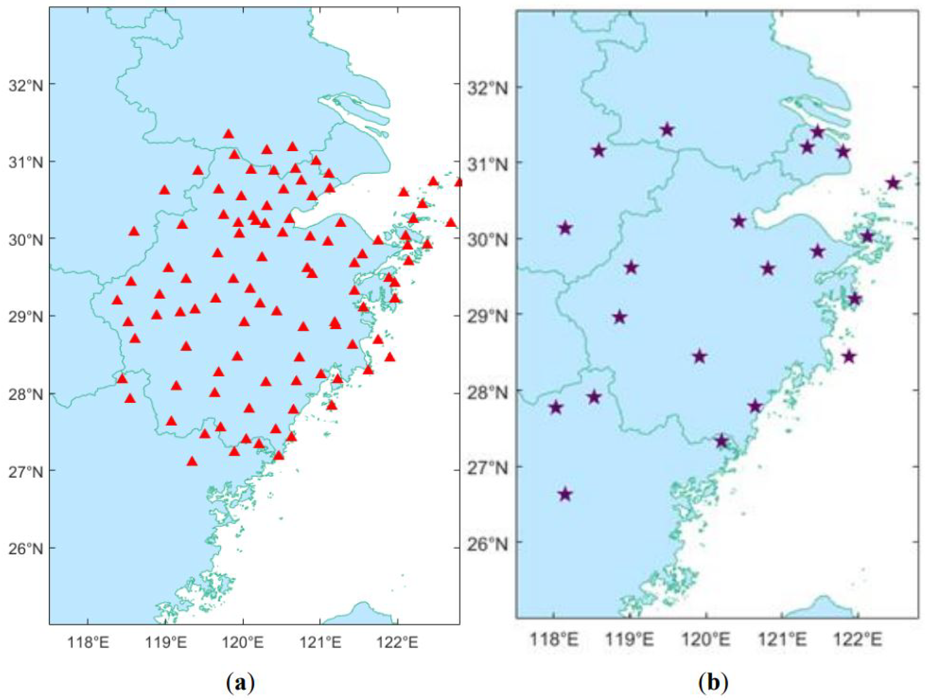
The experimental site studied was mainly located in Zhejiang Province, China, with an area of about 105,500 km 2 . Three data sources were used in the experiment, i.e., the GNSS data from the CORS in Zhejiang, the meteorological data provided by the Zhejiang Meteorological Bureau, and the GPT2w model data. The distribution of CORS locations in Zhejiang is shown in Figure 1a. The CORS network in Zhejiang contains 80 GNSS reference stations, covering Zhejiang Province and surrounding areas. The distribution of the selected meteorological stations in Zhejiang and surrounding areas is shown in Figure 1b, with 21 meteorological stations in total. The meteorological parameters recorded included temperature, atmospheric pressure, and relative humidity. In addition, the latitude of the Zhejiang area ranges from 26.5° to 31.5°, and the longitude ranges from 117.5° to 123.5°. Moreover, 42 evenly distributed grid points were selected according to the horizontal resolution of 1° × 1°, and observations at these points were provided by the GPT2w model.
In this study, the independently researched and developed real-time PPP processing software was deployed at the CORS center in Zhejiang Province and the ZTD of each GNSS station in the Zhejiang CORS was calculated using the IGS RTS real-time orbit clock difference products. The temperature, atmospheric pressure, and relative humidity data recorded at the 21 meteorological stations were used in the Saastamoinen model for ZTD calculations. The GPT2w model provided the ZTD values for the 42 grid points. In this study, the accuracy of the model was evaluated under three different weather conditions, namely the tropospheric quiet period (all sunny days in January 2017), the tropospheric active period (all rainy days in June 2017), and the extreme-weather typhoon period (in September 2017). The fusion modeling was performed at 1 h intervals from UTC 00:00 every day. The ZTD values of 50 GNSS stations were involved in the fusion modeling, and the ZTD values of the remaining GNSS stations were used as standard references to evaluate the accuracy of the fusion model.
At the same time, a PPP tropospheric model was established using the ZTD values of 50 CORS alone, and the GPT2w model directly calculated the ZTD of the inspection station. These results were used together as comparative references in this study. The evaluation criteria are shown in Formula (7):
b i a s = 1 N i = 1 N ( Z T D i e s t i m a t e d Z T D i G N S S d e r i v e d ) R M S = 1 N i = 1 N ( Z T D i e s t i m a t e d Z T D i G N S S d e r i v e d ) 2
The ‘estimated’ represents the ZTD of polynomial models with different coefficients calculated from different data sources. In the subsequent analysis, the results of the fusion model are named “Fusion”, the results of modeling using the ZTD values of GNSS alone are named “PPP”, the results of GPT2w are named “GPT2w”, and the GNSS stations used as references are named “GNSS”.

3. Results

In this section, the accuracy of the fusion model is evaluated under different levels of tropospheric activity, including the tropospheric quiet period, the tropospheric active period, and the typhoon period. Additionally, the accuracy of the fusion model is analyzed for modeling sites with varying levels of sparsity.

3.1. ZTD Inspection

In the following, the accuracy of the models in the tropospheric quiet period, the tropospheric active period, and the typhoon period was tested using the GNSS reference station.

3.1.1. Case Study 1: Tropospheric Quiet Period

The first study period was a tropospheric quiet period, which included all sunny days in January. The GNSS-solved ZTD values of the CORS that were not involved in the modeling were used as independent external references to inspect the accuracy of the tropospheric fusion model.
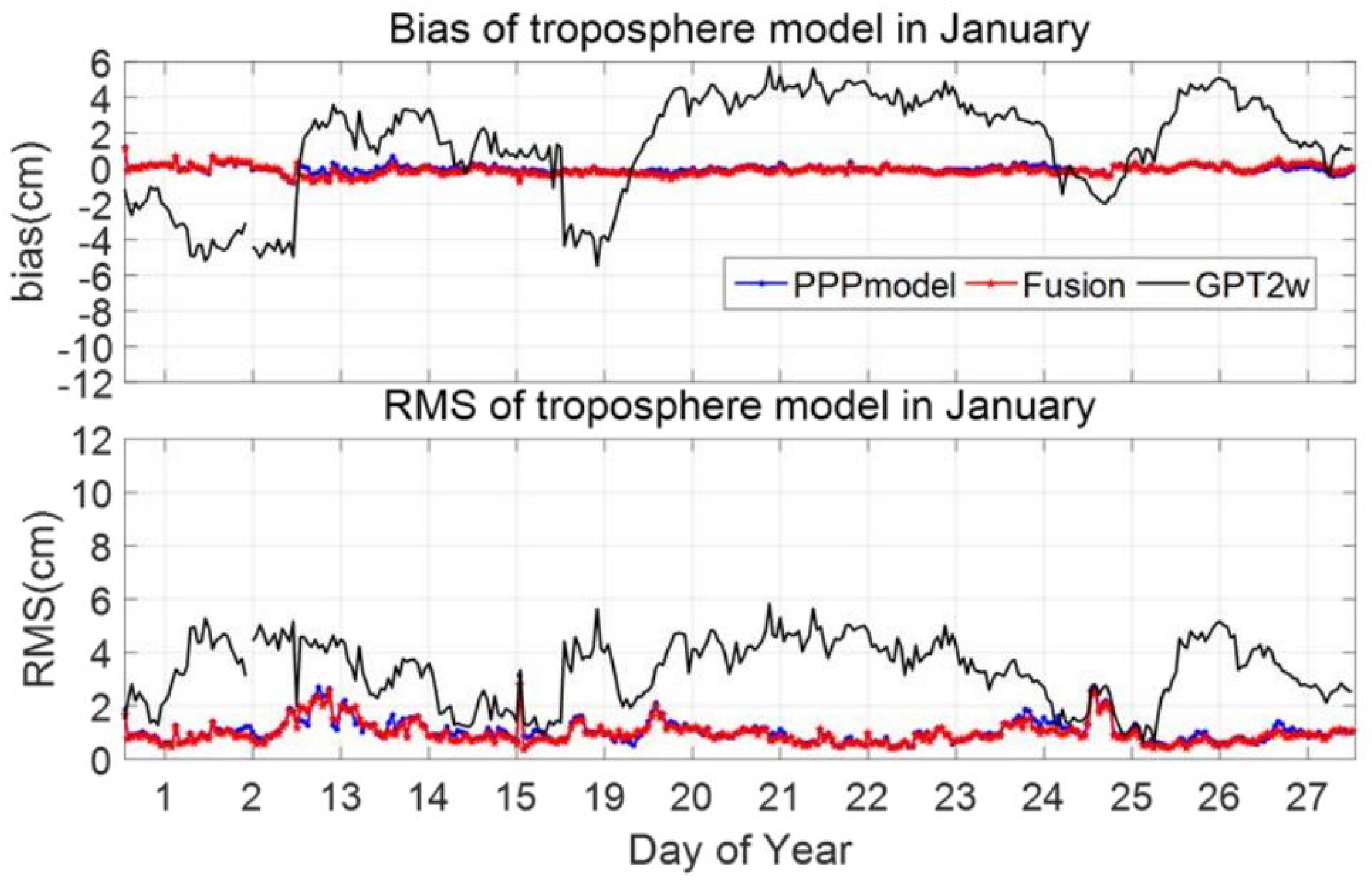
The ZTD series on doy 19 and doy 27 at station ZHJJ estimated by the different models are shown in Figure 2. The mean bias and RMS time series of the external coincidence accuracy at the inspection station of the different tropospheric models, during the tropospheric quiet period in January, are shown in Figure 3. Figure 3 shows that during the sunny days in January, the bias of the ZTD produced by the GPT2w model fluctuated between −5.47 cm and 5.76 cm, and the RMS fluctuated between 0.65 cm and 5.83 cm. As an empirical model, GPT2w did not consider the daily variations in ZTD, and the ZTD values it produced remained constant over a given day. Therefore, the GPT2w model had relatively poor accuracy during this period. In contrast to the empirical model, the accuracy of the PPP model was more reliable. Its bias fluctuated between −0.79 cm and 1.20 cm, and the RMS values were between 0.44 cm and 3.13 cm, which were equivalent to the bias of the fusion model with the highest accuracy. The bias in the ZTD estimated by the fusion model fluctuated between −0.76 cm and 1.15 cm, and the maximum and minimum values of RMS were 2.82 cm and 0.41 cm, respectively. As shown in Figure 3, the fusion model maintained the highest accuracy and stability throughout the tropospheric quiet period.
The daily mean external coincidence accuracy between each model and the GNSS-solved ZTD, and the corresponding bias and RMS, are listed in Table 1. Table 1 shows that the mean RMS of the ZTD fusion model reached 0.96 cm during the tropospheric quiet period, and its accuracy was significantly better than that of the empirical model GPT2w. In comparison with the PPP model, the fusion model had slightly better accuracy, and its GNSS-ZTD spatial resolution was improved.

3.1.2. Case Study 2: Tropospheric Active Period

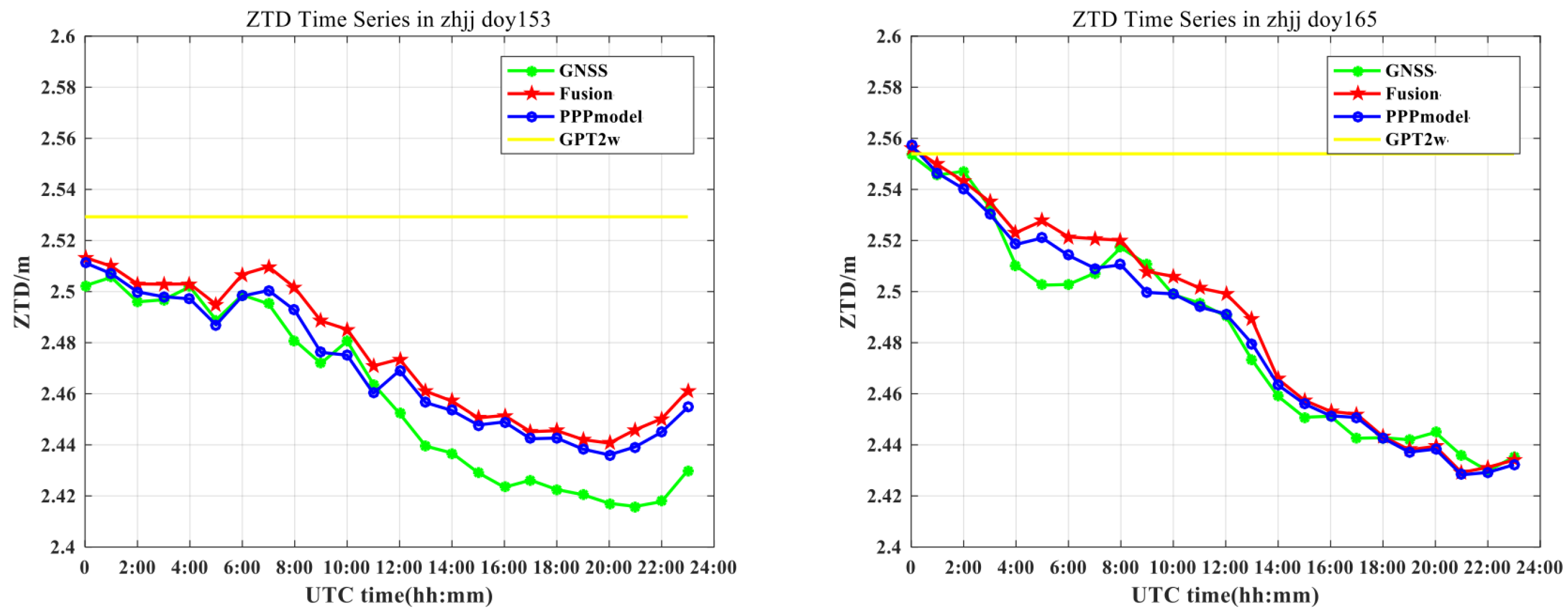
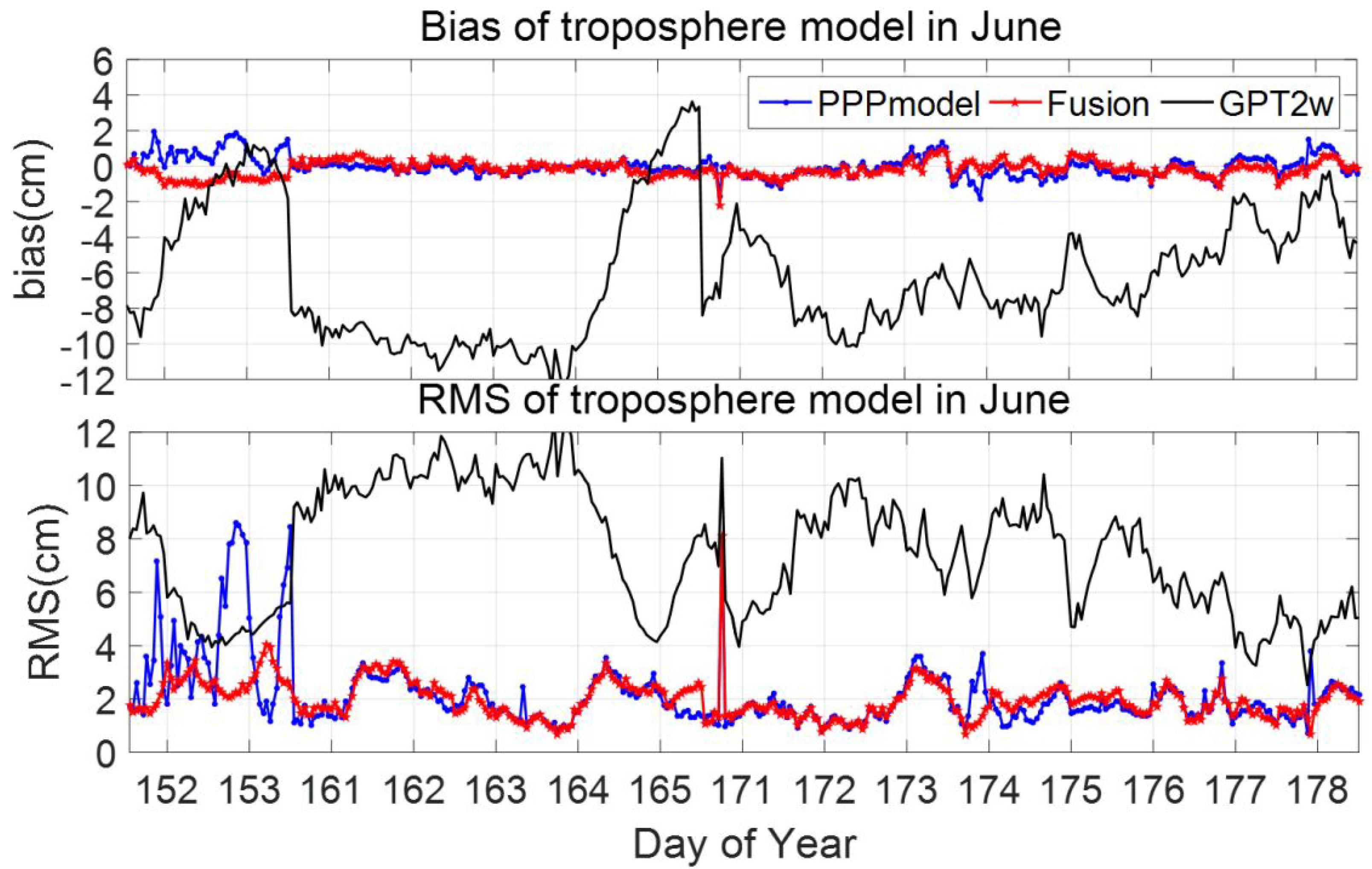
The second study period was a tropospheric active period, which included all rainy days in June, and the regional tropospheric fusion modeling was performed every hour. Similar to the first study period, the GNSS-solved ZTD values of the CORS that were not involved in the modeling were used to evaluate the accuracy of the tropospheric fusion model. Taking the ZTD series of station ZHJJ as an example, the ZTD series on doy 153 and doy 165 at station ZHJJ estimated by the different models are shown in Figure 4. The ZTD values of the fusion model had good agreement with the GNSS-solved ZTD, with mean biases of 1.67 cm and 0.5 cm on doy 153 and doy 165, respectively. For the tropospheric active period of the rainy season in June, the mean bias and RMS time series of the external coincidence accuracy at the inspection station for the different tropospheric models are shown in Figure 5. Figure 5 shows that during the rainy days in June, the bias of the ZTD values produced by the GPT2w model fluctuated between −12.47 cm and 3.63 cm, and the RMS fluctuated between 2.52 cm and 12.50 cm. In contrast to the results for the sunny days, the bias of the GPT2w-modeled ZTD generally exhibited negative values, which means that the ZTD values estimated by the empirical model were generally lower than the actual values on rainy days. Since the GPT2w model is empirical, its accuracy decreases under rainy weather due to the effects of multiple days of rainfall. Therefore, the accuracy of the GPT2w model was relatively poor during this period.
The accuracy of the PPP model, which was modeled using the GNSS-solved ZTD alone, was very high. The bias of this model was between −1.82 cm and 1.94 cm, and the RMS value was between 0.72 cm and 8.60 cm, which is equivalent to the bias of the fusion model with the highest accuracy. The introduction of the empirical model and the meteorological tropospheric data significantly improved the accuracy of the ZTD fusion model. The bias in the ZTD estimated by the fusion model fluctuated between −2.19 cm and 0.91 cm, and the maximum and minimum RMS values were 8.13 cm and 0.64 cm, respectively. The accuracies of ZTD results produced by each model during the tropospheric active period were generally lower than those during the tropospheric quiet period. As shown in Figure 5, the accuracy of the PPP tropospheric model fluctuated greatly between doy 152 and doy 153, while the fusion model maintained the highest accuracy and stability during the tropospheric active period, except for a few moments.
The statistical results of the daily mean bias and RMS of each model at the CORS that were not involved in the modeling are summarized in Table 2. Table 2 shows that during the tropospheric active period, the accuracy of each model was lower than that during the quiet period. When using PPP-ZTD values alone in the modeling, the accuracy was slightly lower than that of the fusion model. As in the first study period, the advantage of the fusion model in terms of accuracy was obvious. The fusion model was significantly more accurate than the empirical model GPT2w. In addition, the fusion model still maintained the highest accuracy and stability during the tropospheric active period, and the modeling costs were reduced via the introduction of meteorological data and the empirical model.

3.1.3. Case Study 3: Typhoon Period

The third study period was a typhoon period with an extremely active troposphere, including three days when the typhoon was passing through (doy 255–doy 257) and a heavy rainstorm period after the typhoon (doy 260–doy 262). The regional tropospheric fusion modeling was performed every hour.
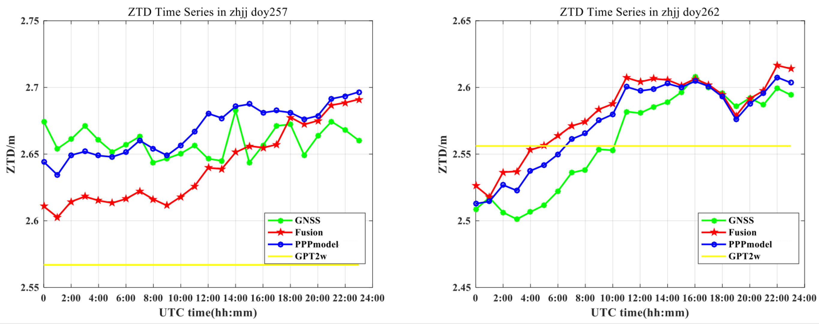
Taking the ZTD series of station ZHJJ as an example, the ZTD series on doy 257 and doy 262 at ZHJJ station estimated by different models are shown in Figure 6. The ZTD values of the fusion model were in good agreement with the GNSS-solved ZTD values, with mean biases of 1.67 cm and 0.5 cm, respectively, while the PPP tropospheric model exhibited the best agreement with the GNSS-solved ZTD.
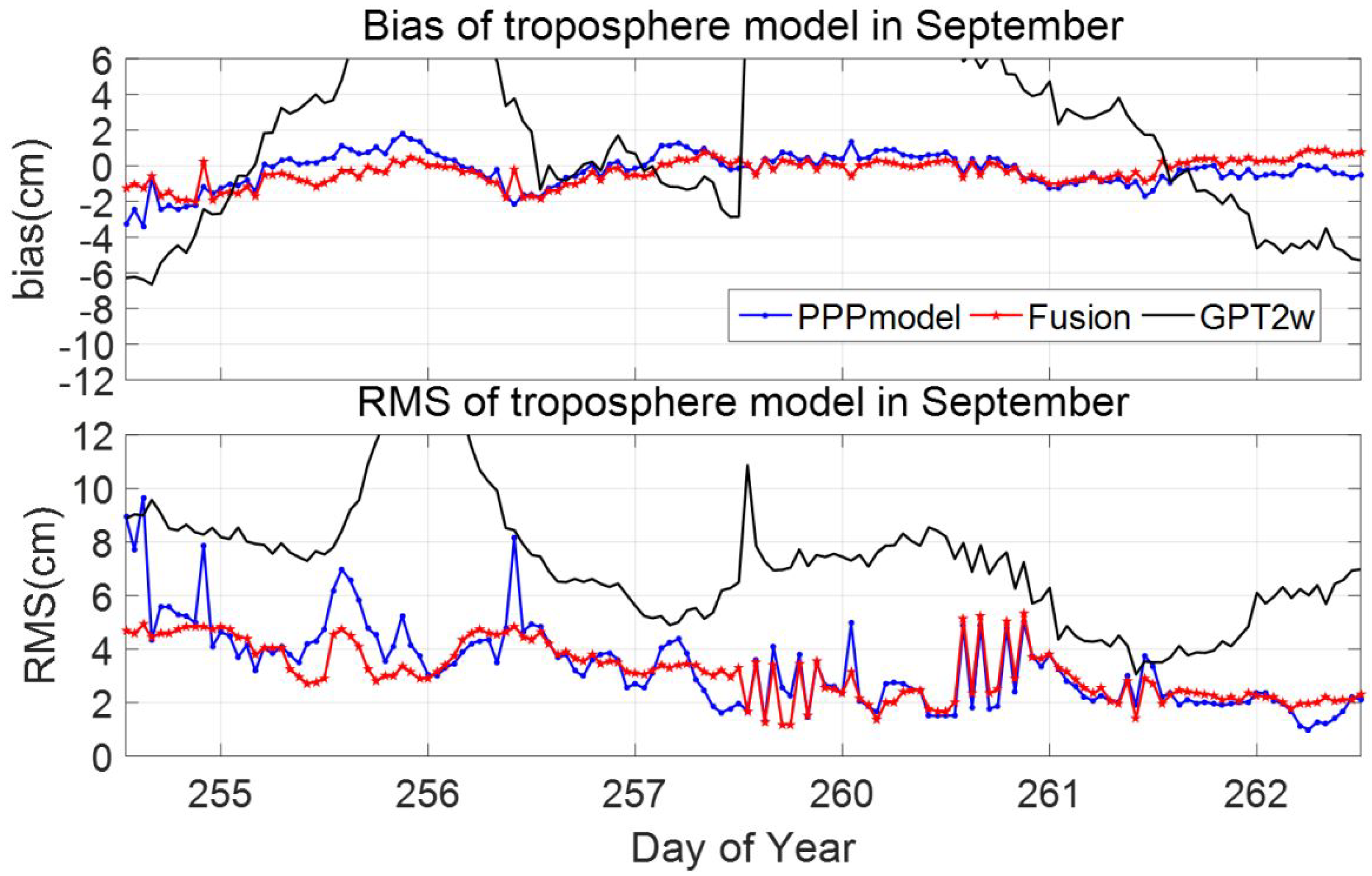
For the tropospheric extreme active period in September, the mean bias and RMS time series of the external coincidence accuracy at the inspection station of the different tropospheric models are shown in Figure 7. Figure 7 shows that during the typhoon period in September, the minimum ZTD bias of the GPT2w model was −6.65 cm, the maximum bias was 14.24 cm, and the RMS fluctuated between 3.05 cm and 14.75 cm. Affected by the typhoon and rainstorm, the accuracy of the empirical model under typhoon conditions was very low. The accuracy of the PPP model, which employed the GNSS-solved ZTD alone, was very reliable. The bias of this model fluctuated between −3.38 cm and 1.77 cm, and the RMS values were between 0.99 cm and 9.66 cm. The fusion model had the highest accuracy of all the models. The introduction of the empirical model and meteorological tropospheric data had a significant stabilizing effect on the accuracy of the ZTD fusion model. The bias of the ZTD estimated by the fusion model fluctuated between −2.03 cm and 0.98 cm, and the maximum and minimum RMS values were 5.31 cm and 1.00 cm, respectively. During the tropospheric active periods, especially the typhoon period, the ZTD predictions of each model were generally less accurate than they were during the tropospheric quiet period. As shown in Figure 7, the accuracy of the PPP tropospheric model fluctuated greatly from doy 152 to doy 153, while the fusion model maintained the highest accuracy and stability during the tropospheric active period, except for a few moments.
Statistical results of the daily mean bias and RMS of each model at the CORS that were not involved in the modeling are summarized in Table 3. During the typhoon period, the fusion model maintained an external coincidence accuracy of about 4 cm. After the typhoon passed through, the external coincidence accuracy of the model improved. During the tropospheric active period, the accuracy of the model, which employed the PPP-ZTD alone, was slightly lower than that of the fusion model. Similar to the first study period, the fusion model still maintained the highest accuracy and stability throughout the tropospheric active period, and the ZTD model’s fusion-based multi-source data were significantly better than the empirical GPT2w model. In addition, the introduction of meteorological data and the empirical model reduced the modeling costs. The tropospheric fusion model had high accuracy in the areas covered by CORS, regardless of whether the tropospheric conditions were quiet or active, including the strong convective typhoon conditions.

3.2. Impact of the Number of Stations on Model Accuracy

The cost of establishing CORS is high, and the coverage of CORS in different areas also varies. In this section, the accuracy of the fusion model under different conditions of the sparseness of modeling sites is evaluated. Moreover, 5 CORS networks with different extents of sparseness were selected for modeling, and the number of stations was 11, 20, 30, 40, and 50, respectively. The modeling accuracy was then inspected using 11 GNSS stations.
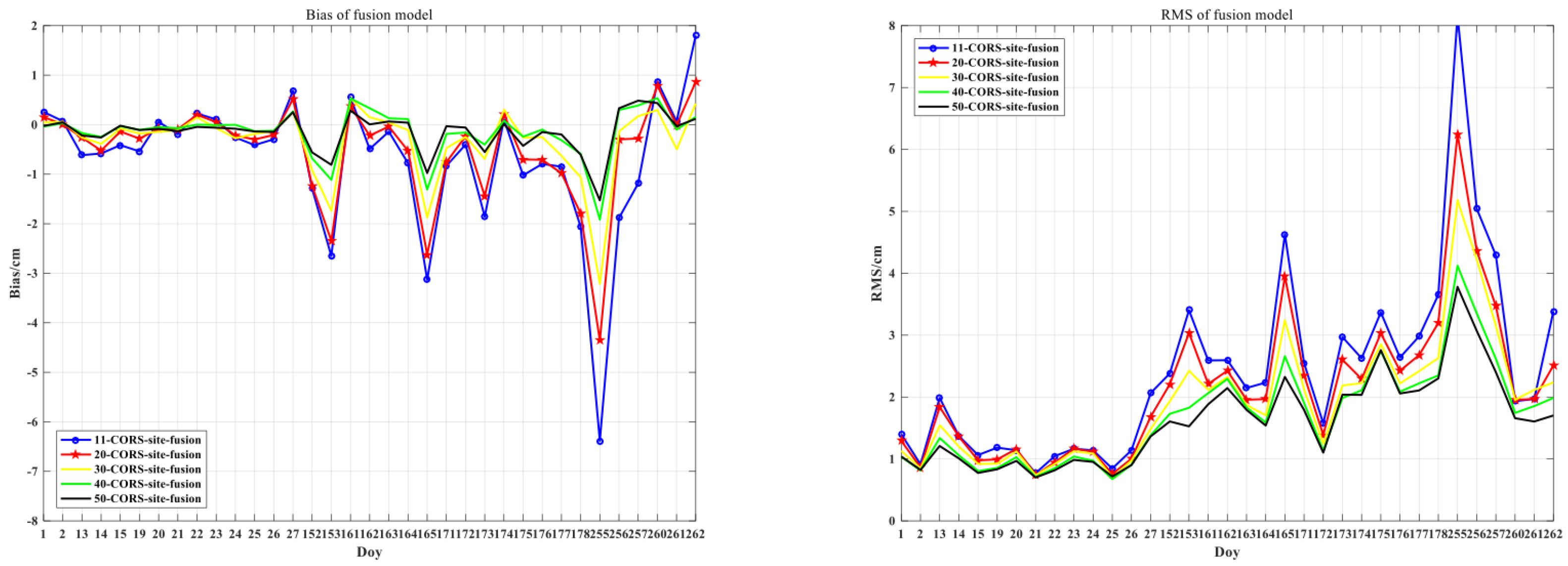
First, the external coincidence accuracies of the fusion models for five different extents of sparseness were calculated, and the external coincidence RMS time series are shown in Figure 8. It can be seen from Figure 8 that the fusion model was more accurate when the density of the stations modeled was higher. The reason for the improved accuracy is that more high-accuracy GNSS ZTD observations were involved in the modeling. In particular, during the period with the extremely active troposphere, the higher density of modeling sites confers great improvements to the model accuracy, which shows that the mathematical fitting still has certain limitations and that increasing the number of physical observations is more effective.
Figure 9 shows the bias and RMS time series to compare the accuracy of the fusion model with that of the PPP model. The comparison reveals the effectiveness of the fusion model in improving the accuracy of the modeling. The figure shows that when the density of GNSS stations is low, the accuracy improvement provided by the multi-source data fusion model is more significant. For an area such as Zhejiang, when the number of CORS is less than 40, the improvement brought about by the multi-source data fusion model is significant in comparison to the results from the GNSS tropospheric model.
Therefore, for areas with a high density of CORS, the GNSS-ZTD data of CORS or the fusion model can be used in modeling to obtain the tropospheric delay results with the highest accuracy and the best horizontal resolution. In areas with sparse CORS coverage, such as marine areas, the use of low-cost meteorological observation equipment and the incorporation of the empirical model to enhance the GNSS network can lead to denser monitoring of the troposphere. This approach can significantly improve the estimation accuracy and horizontal resolution of the tropospheric delay while greatly reducing the modeling costs associated with solving for tropospheric delay.

4. Conclusions

GNSS data processing can provide high-accuracy tropospheric delay information on a global scale. However, the development of the tropospheric model is limited by the uneven distribution and high operation and maintenance costs of CORS. In order to reduce the modeling costs and ensure the accuracy of the tropospheric model, a real-time regional tropospheric fusion model was proposed herein to improve the accuracy and reliability of the tropospheric model in areas with limited GNSS tracking stations. By fusing the ZTD values obtained from the Saastamoinen meteorological model with those obtained from the empirical model GPT2w, the establishment of a tropospheric model with low costs, high spatiotemporal resolution, and high accuracy was achieved. Given the variations in accuracy between different types of tropospheric data, prior accuracies were considered in the Helmert variance component estimation method to determine the weighting of each type of observation data. In addition, the systematic errors of the Saastamoinen model, the GPT2w model, the GNSS model, and the fitting coefficient of the fusion model were estimated by the least-squares method.
The accuracy of the tropospheric fusion model in Zhejiang Province was evaluated during a tropospheric quiet period, a tropospheric active period, and an extreme-weather typhoon period. The observation data of 80 CORS were processed using PPP technology to incorporate it into the modeling data. Moreover, the accuracy of the tropospheric model established using the GNSS observation data alone was investigated in this study. In comparison to the GNSS-solved ZTD, the fusion model established using data from 50 selected CORS had RMS mean accuracies of 0.96 cm during the tropospheric quiet period, 1.92 cm during the tropospheric active period, and 3.11 cm when the typhoon was passing through. The accuracy of the tropospheric fusion model was slightly better than that of the PPP model and significantly better than that of the GPT2w model.
In this study, based on the analysis of the characteristics of three currently available tropospheric delay models and the comparison of their advantages and shortcomings, a real-time study of the observations of the three models was conducted, and a complete set of fusion theories and methods was proposed to establish a real-time multi-source tropospheric fusion modeling system. The new system can process and fuse GNSS observation data, meteorological observation data, and empirical model data in real time, providing a tropospheric fusion model with better accuracy and higher spatiotemporal resolution than those of the individual methods, and at a lower cost. This model can be released to the public through the cloud platform to provide services in many fields such as space radio technology, geodesy, and meteorology. Taking the ZTD time series of station ZHIJ as an example, the ZTD time series on doy 19 and doy 27 calculated by the fusion model, the PPP model, and the GPT2w model are shown in Figure 3. It can be seen from the figure that as an empirical model, GPT2w produced ZTD values with very small variations during the day, staying close to a constant value. Since the fusion model was mainly based on the GNSS observation data, the variations in ZTD can be in very good agreement with those of GNSS-ZTD, and the maximum bias from the GNSS-ZTD values did not exceed 2 cm.

Author Contributions

Methodology, C.X., J.K., Y.Y. and J.S.; Validation, X.X.; Investigation, J.K.; Resources, Y.Z.; Data curation, X.L.; Writing—original draft, C.X.; Supervision, Y.Y. All authors have read and agreed to the published version of the manuscript.

Funding

This research was funded by the National Natural Science Foundation of China (nos. 41721003, 41874033, 41804038, 42004019, and 41604002).

Institutional Review Board Statement

Not applicable.

Informed Consent Statement

Informed consent was obtained from all subjects involved in the study.

Data Availability Statement

The data used to support the findings of this study are available from the corresponding author upon request.

Conflicts of Interest

The authors declare no conflict of interest.

References

  1. Kursinski, E.; Hajj, G.; Hardy, K.; Romans, L.; Schofield, J. Observing tropospheric water vapor by radio occultation using the Global Positioning System. Geophys. Res. Lett. 1995, 22, 2365–2368. [Google Scholar] [CrossRef]
  2. Kouba, J.; Héroux, P. Precise point positioning using IGS orbit and clock products. GPS Solut. 2001, 5, 12–28. [Google Scholar] [CrossRef]
  3. Ware, R.; Alber, C.; Rocken, C.; Solheim, F. Sensing integrated water vapor along GPS ray paths. Geophys. Res. Lett. 1997, 24, 417–420. [Google Scholar] [CrossRef]
  4. Bar-Sever, Y.E.; Kroger, P.M.; Borjesson, J.A. Estimating horizontal gradients of tropospheric path delay with a single GPS receiver. J. Geophys. Res. Solid Earth 1998, 103, 5019–5035. [Google Scholar] [CrossRef]
  5. Collins, J.P.; Langley, R.B. A Tropospheric Delay Model for the User of the Wide Area Augmentation System; Department of Geodesy and Geomatics Engineering, University of New Brunswick: Fredericton, NB, Canada, 1997. [Google Scholar]
  6. Böhm, J.; Niell, A.; Tregoning, P.; Schuh, H. Global Mapping Function (GMF): A new empirical mapping function based on numerical weather model data. Geophys. Res. Lett. 2006, 33, L07304. [Google Scholar] [CrossRef]
  7. Böhm, J.; Heinkelmann, R.; Schuh, H. Short note: A global model of pressure and temperature for geodetic applications. J. Geod. 2007, 81, 679–683. [Google Scholar] [CrossRef]
  8. Kouba, J. Testing of global pressure/temperature (GPT) model and global mapping function (GMF) in GPS analyses. J. Geod. 2009, 83, 199–208. [Google Scholar] [CrossRef]
  9. Lu, C.; Zus, F.; Ge, M.; Heinkelmann, R.; Dick, G.; Wickert, J.; Schuh, H. Tropospheric delay parameters from numerical weather models for multi-GNSS precise positioning. Atmos. Meas. Tech. 2016, 9, 5965–5973. [Google Scholar] [CrossRef]
  10. Lagler, K.; Schindelegger, M.; Böhm, J.; Krásná, H.; Nilsson, T. GPT2: Empirical slant delay model for radio space geodetic techniques. Geophys. Res. Lett. 2013, 40, 1069–1073. [Google Scholar] [CrossRef]
  11. Böhm, J.; Möller, G.; Schindelegger, M.; Pain, G.; Weber, R. Development of an improved empirical model for slant delays in the troposphere (GPT2w). GPS Solut. 2015, 19, 433–441. [Google Scholar] [CrossRef]
  12. Landskron, D.; Böhm, J. VMF3/GPT3: Refined discrete and empirical troposphere mapping functions. J. Geod. 2018, 92, 349–360. [Google Scholar] [CrossRef] [PubMed]
  13. Hopfield, H. Two-quartic tropospheric refractivity profile for correcting satellite data. J. Geophys. Res. 1969, 74, 4487–4499. [Google Scholar] [CrossRef]
  14. Qu, W.; Zhu, W.; Song, S.; Ping, J. The evaluation of precision about Hopfield, Saastamoinen and EGNOS tropospheric delay correction model. Acta Astron. Sin. 2008, 49, 113–122. [Google Scholar]
  15. Black, H.D. An easily implemented algorithm for the tropospheric range correction. J. Geophys. Res. Solid Earth 1978, 83, 1825–1828. [Google Scholar] [CrossRef]
  16. Satirapod, C.; Chalermwattanachai, P. Impact of different tropospheric models on GPS baseline accuracy: Case study in Thailand. J. Glob. Position. Syst. 2005, 4, 36–40. [Google Scholar] [CrossRef]
  17. Tuka, A.; El-Mowafy, A. Performance evaluation of different troposphere delay models and mapping functions. Measurement 2013, 46, 928–937. [Google Scholar] [CrossRef]
  18. Saastamoinen, J. Atmospheric correction for the troposphere and stratosphere in radio ranging satellites. Artif. Satell. Geod. 1972, 15, 247–251. [Google Scholar]
  19. Tao, W. Near Real-Time GPS PPP-Inferred Water Vapor System Development and Evaluation. Master’s Thesis, Department of Geomatics Engineering, University of Calgary, Calgary, AB, Canada, 2008. [Google Scholar]
  20. Ye, S.; Zhang, S.; Liu, J. Precision analysis of precise point positioning based tropospheric delay estimation. Geomat. Inf. Sci. Wuhan Univ. 2008, 33, 788–791. [Google Scholar]
  21. Laurichesse, D.; Mercier, F.; BERTHIAS, J.P.; Broca, P.; Cerri, L. Integer ambiguity resolution on undifferenced GPS phase measurements and its application to PPP and satellite precise orbit determination. Navigation 2009, 56, 135–149. [Google Scholar] [CrossRef]
  22. Wang, M.; Chai, H.; Xie, K.; Chen, Y. PWV inversion based on CNES real-time orbits and clocks. J. Geod. Geodyn. 2013, 33, 137–140. [Google Scholar]
  23. Shi, J.; Xu, C.; Guo, J.; Gao, Y. Local troposphere augmentation for real-time precise point positioning. Earth Planets Space 2014, 66, 30. [Google Scholar] [CrossRef]
  24. Askne, J.; Nordius, H. Estimation of tropospheric delay for microwaves from surface weather data. Radio Sci. 1987, 22, 379–386. [Google Scholar] [CrossRef]
  25. Teunissen, P.J.; Amiri-Simkooei, A. Least-squares variance component estimation. J. Geod. 2008, 82, 65–82. [Google Scholar] [CrossRef]
Figure 1. Continuously operating reference station(s) (CORS) in Zhejiang (a) and meteorological stations in Zhejiang (b).
Atmosphere 14 00815 g001
Figure 2. GNSS-derived ZTD and ZTD estimated by different models at station ZHIJ on doy 19 and 27.
Atmosphere 14 00815 g002
Figure 3. Bias and RMS of each tropospheric model in January.
Atmosphere 14 00815 g003
Figure 4. GNSS-derived ZTD and ZTD estimated by different models at station ZHIJ on doy 153 and doy 165.
Atmosphere 14 00815 g004
Figure 5. Bias and RMS of each tropospheric model in June.
Atmosphere 14 00815 g005
Figure 6. GNSS-derived ZTD and ZTD estimated by different models at station ZHIJ on doy 257 and doy 262.
Atmosphere 14 00815 g006
Figure 7. Bias and RMS of each tropospheric model in September.
Atmosphere 14 00815 g007
Figure 8. Bias and RMS of the fusion model.
Atmosphere 14 00815 g008
Figure 9. Bias and RMS of the fusion model and the PPP model.
Atmosphere 14 00815 g009
Table 1. Daily mean external accuracy (cm) of tropospheric models in January.
DoyFusionPPPGPT2w
BiasRMSBiasRMSBiasRMS
1 *0.140.790.130.85−2.822.97
20.111.010.051.12−4.154.28
13−0.491.71−0.111.642.143.73
14 *−0.120.970.091.131.982.57
15−0.220.81−0.080.981.041.68
19−0.220.98−0.161.00−2.373.37
20 *−0.281.14−0.121.193.794.07
21−0.050.820.030.904.484.58
22 *−0.060.59−0.010.634.204.31
23 *−0.170.86−0.050.893.613.77
24−0.131.140.061.351.342.38
25−0.071.02−0.041.120.311.86
26 *0.080.650.050.734.304.40
270.140.94−0.061.021.492.94
mean−0.100.96−0.021.041.383.35
Table 2. Daily mean external accuracy (cm) of tropospheric models in June.
DoyFusionPPPGPT2w
BiasRMSBiasRMSBiasRMS
152 *−0.592.330.593.22−5.376.59
153−0.472.220.844.92−0.074.71
1610.341.990.001.85−8.909.60
162 *0.162.65−0.112.41−10.2810.73
163−0.061.53−0.291.79−10.2310.39
164 *−0.011.83−0.101.90−9.4210.01
165−0.301.97−0.071.930.725.81
171−0.531.78−0.471.75−5.136.13
172 *−0.371.18−0.281.20−8.798.95
1730.092.260.422.38−7.457.99
1740.051.61−0.601.67−7.268.01
175 *0.152.12−0.301.77−6.567.50
176−0.261.84−0.301.81−6.397.05
177−0.321.63−0.031.69−3.744.91
178 *−0.091.820.281.95−2.924.82
mean−0.151.92−0.032.15−6.127.55
Table 3. Daily mean external accuracy (cm) of tropospheric models in September.
DoyFusionPPPGPT2w
BiasRMSBiasRMSBiasRMS
255−1.084.21−1.185.08−1.498.25
256 **−0.393.910.214.638.6911.13
257−0.323.230.033.23−0.636.00
2600.072.210.512.507.337.76
261 *−0.603.17−0.622.964.035.52
2620.181.93−0.371.87−3.065.24
mean−0.363.11−0.243.382.487.32
Disclaimer/Publisher’s Note: The statements, opinions and data contained in all publications are solely those of the individual author(s) and contributor(s) and not of MDPI and/or the editor(s). MDPI and/or the editor(s) disclaim responsibility for any injury to people or property resulting from any ideas, methods, instructions or products referred to in the content.