Article

Variations in CO2 and CH4 Exchange in Response to Multiple Biophysical Factors from a Mangrove Wetland Park in Southeastern China

1
Guangzhou Climate and Agrometeorology Center, Guangzhou 510080, China
2
Southern Marine Science and Engineering Guangdong Laboratory (Zhuhai), Zhuhai 519000, China
3
Key Laboratory of Watershed Geographic Sciences, Nanjing Institute of Geography and Limnology, Chinese Academy of Sciences, Nanjing 210008, China
4
State Key Laboratory of Atmospheric Boundary Layer Physics and Atmospheric Chemistry, Institute of Atmospheric Physics, Chinese Academy of Sciences, Beijing 100029, China
5
National Climate Center, China Meteorological Administration, Beijing 100081, China
6
Guangxi Meteorological Service, Nanning 530022, China
7
Guangxi Institute of Meteorological Sciences, Nanning 530022, China
*
Author to whom correspondence should be addressed.
Atmosphere 2023, 14(5), 805; https://doi.org/10.3390/atmos14050805
Submission received: 9 March 2023 / Revised: 25 April 2023 / Accepted: 26 April 2023 / Published: 28 April 2023
(This article belongs to the Section Biosphere/Hydrosphere/Land–Atmosphere Interactions)

Abstract

:
Mangrove ecosystems can be both significant sources and sinks of greenhouse gases. The restoration of mangrove forests is increasingly used as a natural climate solution tool to mitigate climate change. However, the estimates of carbon exchanges remain unclear, especially from restored mangroves. In this study, we observed the temporal variations in carbon dioxide (CO2) and methane (CH4) fluxes and their biophysical controls for 4 years, based on a closed-path eddy covariance (EC) system. The measurements were conducted in a mangrove wetland park with 14-year-old restored mangroves surrounded by open waters in Guangdong Province, China. The EC measurements showed that the mangrove ecosystem acted as a CO2 source with a net CO2 ecosystem exchange (NEE) of 305 g C m−2 from January 2019 to May 2020 by the 5-m tower measurement. After the tower was adjusted to 10 m, the mangrove showed a CO2 sink with an NEE of −345 g C m−2 from June 2020 to December 2022. The change in tower height influenced the interpretation of interannual trends on NEE. There were no significant interannual trends in the gross primary productivity (GPP) and the ecosystem respiration (Re) values. The change from CO2 source to sink may be attributed to the decrease in land surface proportion by the tower replacement, which reduces the proportion of the mangrove canopy respiration and, therefore, captures lower CO2 fluxes from open waters. The restored mangroves indicated strong CH4 sources of 23.2–26.3 g C m−2 a−1. According to the random forest analysis, the land surface proportion, radiation, and relative humidity were the three most important predictors of NEE, while the CH4 flux was most sensitive to air temperature. Compared to the natural and long-term restored mangroves, this 14-year-old restored mangrove had not yet achieved a maximum carbon sequestration capability. Our study highlights the need for the careful design of long-term observations from restored mangroves and proposes future needs in the context of carbon neutrality.

1. Introduction

Mangroves are now widely valued and increasingly recognized for their contributions to human society. On the one hand, they can provide ecological services and economic value, such as coastal protection, water purification, and fish biomass production [1,2]. Furthermore, mangroves have the capability to sequester carbon at very large rates per unit area [3,4]. The mean global burial rate of mangroves is 174 g C m−2 y−1, which is triple to tenfold that of other ecosystems [5]. However, their anoxic environment generates CH4 emissions from mangroves, which partially offset “blue carbon” burial in mangroves [6].
The CO2 and CH4 fluxes between the atmosphere and biosphere from mangroves depend on photosynthesis, autotrophic and heterotrophic respiration, and the microbial methanogenic processes [7,8]. Similar to other tropical forests, these processes are greatly influenced by climate factors such as temperature, precipitation, radiation, etc. For example, the temperature regulates stomatal conductance and microbial activity that strongly affect photosynthesis [9], mineralization, and methanogenesis [10]. Precipitation changes the inundation period and indirectly influences the organic matter decomposition [11]. The radiation determines the amount of light available for photosynthesis [12]. Additionally, since mangroves are distributed in coastal tropical and subtropical regions, their carbon fluxes also respond to tidal amplitude [13], salinity [14], and nutrient availability [15].
Mangroves not only support numerous ecosystem services, including fisheries production and nutrient cycling, but also sequester carbon that is disproportionate to their area. As one of the effective natural climate solutions to achieve carbon neutrality [16], mangrove conservation and mangrove restoration have long been recognized by national governments through international agreements. The Chinese mangrove area has increased from 18,602 ha to 28,010 ha from 2000 to 2020, becoming one of the few countries in the world with a net increase in mangrove areas [17,18]. The Mangrove Protection and Restoration Action Plan (2020–25) (MPRAP) issued by China’s Ministry of Natural Resources and the National Forestry and Grassland Administration states that China will restore 9050 ha of mangrove forests, a quarter of which will be carried out in Guangdong Province.
Guangdong Province has the largest mangrove area in China [17]. Many mangrove wetland parks have been established in Guangdong Province since it is a direct and effective way to expand mangrove areas. Mangroves were restored or replanted along open water in these parks. The carbon budgets of mangrove parks are not only influenced by the above climate and environmental factors, but are also related to the recovery period and method, biophysical conditions [19,20], and the proportion of vegetation and open water area [21]. The carbon fluxes from artificially restored mangrove parks have been far less studied than those from natural mature mangroves in China [13,14,22,23,24,25]. It is urgent to estimate the carbon budget due to mangrove restoration to better understand their potential contribution to carbon neutrality on regional or national scales [26].
In this study, we used EC measurements to observe CO2 and CH4 exchanges from a mangrove park having a 12-year restoration period located in Guangzhou, Guangdong Province, China. We analyzed the long-term measurements of CO2 sequestration by plants, CO2 release from plants, open water, and soil respiration, as well as CH4 emissions. The primary objectives were (1) to characterize the temporal variations in CO2 and CH4 fluxes and (2) to reveal the response of carbon fluxes to biophysical drivers.

2. Materials and Methods

2.1. Study Sites

The Nansha Wetland Park (22.60° N, 113.64° E, Figure 1) is located at the mouth of the Pearl River in the southernmost part of Guangzhou, China. It is the largest coastal wetland in Guangzhou and the main area for artificial mangrove restoration. The study site has a subtropical marine monsoon climate, the annual mean temperature is 21.8 °C, and the annual precipitation is 1635.6 mm [27]. The dominant wind direction is northwest in winter and southeast in summer. The park has a total area of approximately 6.54 km2. The dominant tree species at the site are Hibiscus tiliaceus (70%) and Sonneratia apetala (17%), which were artificially restored in 2008. The H. tiliaceus community has a canopy height of 3–4 m and a canopy density of 70%–80%. The mangrove stands were planted in striped shapes surrounded by open waters. The proportion of vegetation canopy is approximately 50%–60%. The Nansha Wetland Park was transformed by artificial reclamation into a tidal flat, which is separated from seawater by levees. Therefore, the site is weakly affected by tides, and the water level changes with only minor fluctuations.

2.2. Flux and Meteorological Measurements

Based on the vegetation and wind patterns, a 5-m flux tower was installed in the center of the wetland park in 2019 (Figure 1). As the mangrove stands grew, the tower was adjusted to 10 m in June 2020. An eddy covariance (EC) system was mounted on the top of the tower. The system consisted of a close-path infrared gas analyzer (GGA, ABB-Los Gatos Research, Mountain View, CA, USA) and a three-dimensional sonic anemometer (WindMaster Pro, Gill Instruments, Lymington, UK). The H2O, CO2, and CH4 flux measurements were recorded by a CR3000 datalogger at a 10 Hz frequency. The environmental variables were measured above the canopy and averaged over 30 min on a CR1000 datalogger. These measurements include air temperature (Ta) and relative humidity (RH) (HMP155, Vaisala Inc., Helsinki, Finland), wind speed (WS), and wind direction (WD) (03002, RM Young, Inc. Traverse City, MI, USA). Soil temperature (Ts), soil moisture (SWC), and soil salinity (Hydra Prob II, Campbell Scientific Inc., Logan, UT, USA) were measured 5 cm below the soil surface. A water-level probe (CS456, Campbell Scientific Inc., Logan, UT, USA) was installed below the water surface inside a 1-m tube, and the water level and water temperature were measured every 30 min. Data were collected from 2019 to 2022 in this study.
Additional meteorological data, including rainfall and sunshine duration, were obtained from a nearby (within 1 km) standard meteorological station (Shijiuchong). The solar radiation data were collected from the Guangzhou national meteorological station (23°08′ N, 113°19′ E). The 4-day leaf area index (LAI) data from 2019 to 2022 were extracted from the MCD15A3H product (250 m) (available online at http://www.glass.umd.edu/LAI/MODIS/250m/, accessed on 20 January 2023). The data were first quality assured based on the product quality control (QC) flag, and were then excluded for outliers considering the weak LAI seasonality of mangroves. Thereby, the low-quality (QC > 32 or LAI < 0.2) LAI data were removed. The preprocessed LAI data were then linearly interpolated to a daily timescale, and the time-series data were smoothed based on a Savitzky–Golay filtering approach [28]. The filtering used cubic polynomials to reconstruct LAI data in a 91-day (3-month) time window. The specific time window was selected as it produced low-noise and plausible LAI time series [28].
The footprints of flux observation varied with the heights of the tower. The footprint of the 5-m tower ranged from 100 m to 200 m [29], which covered approximately 60% of the mangrove stands and 40% of the open waters and fish ponds. The footprint extended to the surrounding of 500–600 m when the tower was raised to a height of 10 m, with an underlying surface of 50% mangrove stands and almost 50% open waters and fish ponds.

2.3. Flux Data Processing and Gap Filling

Postprocessing of flux data followed the FLUXNET standard procedures using EddyPro software v6.1.0. Data processing consisted of spike removal [30], angle-of-attack correction for Gill anemometers [31], a two-dimensional coordinate rotation [32], a time lag correction of CO2 concentration to maximize covariance with vertical wind speed variation [33], buoyancy corrections of sonic air temperatures [34], and WPL correction for air density fluctuations [35]. According to the friction velocity, the night time flux data affected by weak turbulence were eliminated based on the friction velocity (u*) [36]. The 30-min fluxes were also rejected if the quality flags were equal to 1 or 2, in accordance with the method of Mauder and Foken [37].
In addition to periods of mechanical failure and maintenance, data processing (quality flag correction, u* threshold correction, and footprint correction) produced gaps that needed to be filled to integrate the CO2 fluxes on an annual scale. The gaps represented 33% and 38% of the CO2 and CH4 flux data, respectively.
The gaps were filled by using linear interpolation and mean diurnal course methods [38] when gaps were less than 8 h; otherwise, the random forest algorithm was selected to fill the gaps [39]. The gap-filled flux data were used to calculate the monthly and annual carbon source or sink values.

2.4. Flux Partitioning

The CO2 flux data after u* threshold correction were partitioned into gross primary productivity (GPP) and ecosystem respiration. The gross primary production (GPP) was calculated using Equation (1):
GPP = −NEE + Reco
NEE is the net ecosystem exchange, and Reco is the ecosystem respiration. Night time NEE is generally used as a proxy for Reco. In mangroves, Reco is representative of NEE only during emersion periods [40].
The reliable night time data (i.e., after the removal of low turbulent flux data) were regressed with air temperature using the Lloyd–Taylor regression model [41]. The air temperature was used as a proxy for ecosystem respiration to estimate daily respiration rates over a 14-day period. Reco was calculated using Equation (2):
Reco   =   Rref × Ea R 1 Tref 1 T
Reco is the ecosystem respiration, Rref is the ecosystem respiration at 20 °C, Ea is the apparent activation energy (J mol−1), R is the universal gas constant (J mol−1 K−1), Tref is the reference temperature (20 °C, in K), and T is the absolute temperature (K).

3. Results and Discussion

3.1. Temporal Variations in Environmental Conditions

The 4-year in situ observations had strong seasonal variations in most of the environmental factors, such as air and soil temperature (Ta and Ts), precipitation (P), vapor pressure deficit (VPD), relative humidity (RH), solar radiation (Ra), and leaf area index (LAI) (Figure 2a–h). The variations in daily Ta had the highest values at approximately 30 °C in July and the lowest values at approximately 15 °C in January or February due to the typical subtropical monsoon climate (Figure 2a). The annual mean temperature was approximately 24 °C and indicated no significant differences between years (Table 1). The Ts values had variations similar to those of Ta but had less day-to-day variability than Ta (Figure 2a). Most of the precipitation was concentrated from April to September, which accounted for 67–87% of the annual total precipitation.
The highest precipitation was found in August 2019 (412.8 mm), May 2020 (286.5 mm), June 2021 (359.0 mm), and May 2022 (485.1 mm) (Figure 2b). The daily soil salinity ranged from 2.1 ppt to 19.3 ppt from July 2021 to the end of 2022, respectively. The trend of soil salinity was influenced by rainfall events and river water input. Higher salinity values ranging from 14 ppt to 17 ppt were found from December 2021 to mid-February 2022 as well as in October 2022. These were accompanied by lower precipitation (Figure 2b).
The seasonal variations in daily VPD and RH showed approximately opposite variation trends in response to precipitation (Figure 2c,d). Higher precipitation increased RH but reduced VPD. Consistent with the seasonal trend of precipitation, lower RH occurred in the period between October and March in the next year, with daily bottom values of approximately 0.3 (Figure 2d). The average monthly VPD ranged from 0.22 kPa to 1.32 kPa during the past 4 years, with a daily peak at 2.29 kPa in September 2022 (Figure 2c). As shown in Table 1, the climatic conditions in 2019 and 2022 were relatively wetter than those in 2020 and 2021, with higher annual precipitation of 2085.70 mm and 1921.20 mm, higher annual mean RH values of 0.82 and 0.80, and lower VPD values of 0.56 kPa and 0.59 kPa in 2019 and 2022, respectively.
The seasonal variations in the daily Ra and LAI values (Figure 2e,f) also showed seasonal variations, but were weaker than those in temperature (Figure 2a). The daily Ra values were generally higher in summer (178.80 ± 70.16 Wm−2) and lower in winter (126.75 ± 58.64 Wm−2). However, in 2020, 2021, and 2022, the Ra values were low in summer due to continuous precipitation, which resulted in M-shaped patterns in these years (Figure 2e). The daily LAI had general unimodal patterns in 2019, 2020, and 2022 and an obvious M-shaped pattern in 2021 (Figure 2f). In 2019, 2020, and 2022, the monthly mean peaks occurred in September (1.49), August (1.68), and September (1.80), respectively. In 2022, two peaks of monthly mean values of 1.20 and 1.22 were found in July and September (Figure 2f).
There were no significant seasonal variations in the wind speed and the proportion of open water (Figure 2g,h). The wind speed ranged from 1.18 m s−1 to 9.70 m s−1 (Figure 2g). The proportion of open water was determined by the wind speed, wind direction, and tower height. The land surface (Pl) accounted for 62% and 63% in the last 2 years, which was lower than that found in the first 2 years (Table 1).

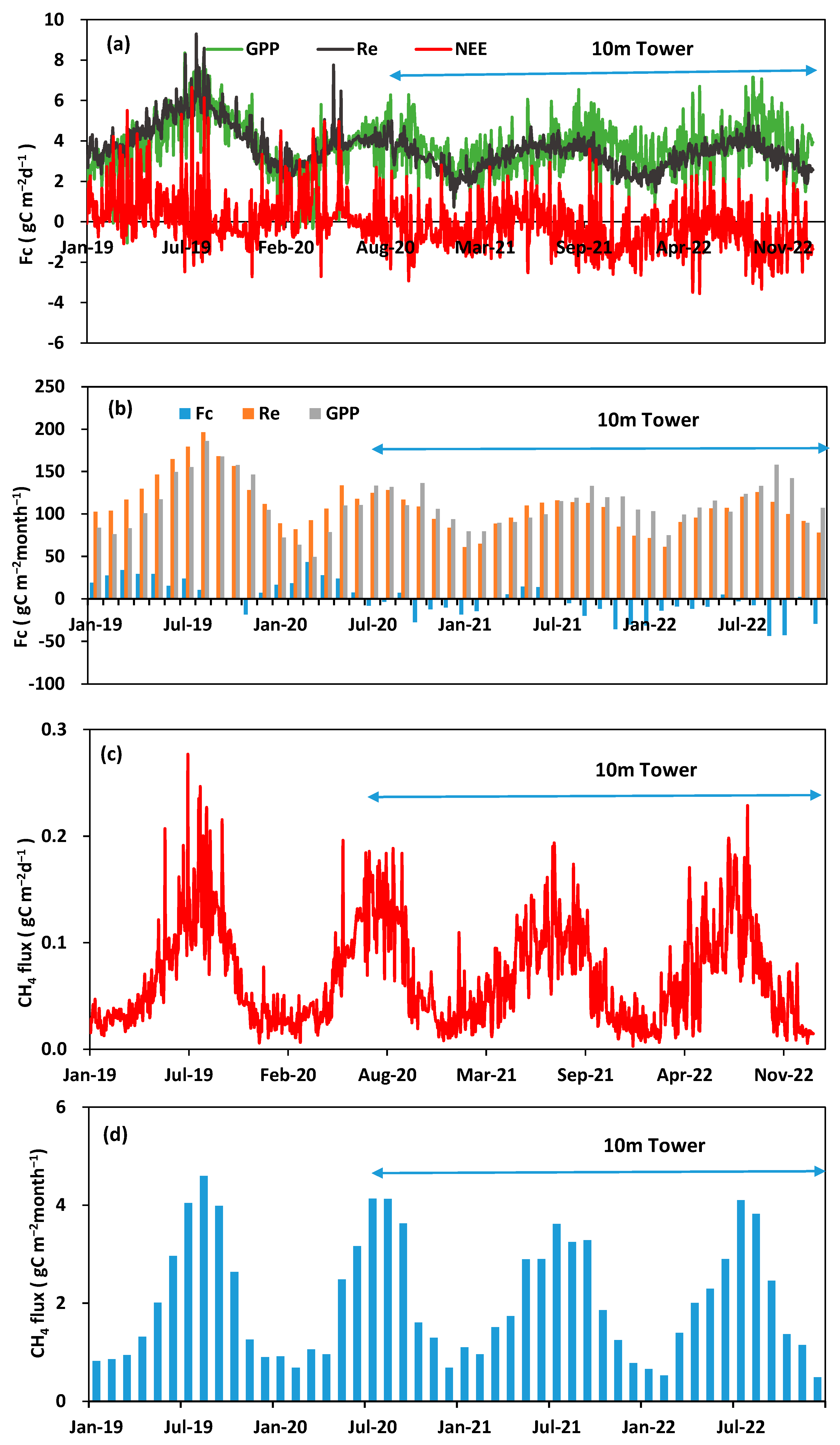
3.2. Seasonal and Interannual Variations in Carbon Fluxes

The daily mean NEE strongly fluctuated between −3.51 g C m−2 d−1 and 6.57 g C m−2 d−1, with negative values (CO2 uptake) accounting for approximately half (Figure 3a). The monthly mean NEE values were positive (CO2 emissions) most of the time in 2019 (from January to September and December) and 2020 (from January to June and September) (Figure 3b). However, the positive monthly mean NEE values only occurred from April to July in 2021, as well as June and November in 2022 (Figure 3b). The highest positive NEE values often occurred in the spring (March in 2019 and 2020, May in 2021) and the summer (June in 2022), with monthly means of 33.93, 43.06, 14.27, and 4.73 g C m−2 mon−1 from 2019 to 2022, respectively. In contrast, the measurements indicated the strongest net CO2 uptake in autumn, with the highest monthly mean values of −18.54 g C m−2 mon−1 in November 2019, −27.56 g C m−2 mon−1 in October 2020, −35.58 g C m−2 mon−1 in November 2021, and −43.65 g C m−2 mon−1 in September 2022 (Figure 3b).
The long- and short-term variations in the NEE values were determined by photosynthesis and respiration. The daily GPP and Re displayed strong seasonal variabilities during the last 4 years, with relatively higher and lower values during summertime and wintertime (Figure 3a), respectively. The strongest daily GPP ranged between 4.37 g C m−2 d−1 and 9.28 g C m−2 d−1. Although the GPP had a strong carbon uptake (49.28–185.72 g C m−2 mon−1) in the spring and summer, Re (88.55–196.27 g C m−2 mon−1) offset or surpassed it most of the time in the first 3 years and finally resulted in a net carbon release. However, the Re values (84.94–167.93 g C m−2 mon−1) were weaker than the GPP values (89.45–167.97 g C m−2 mon−1) most of the time in autumn, which led to a net carbon sink in this season (Figure 3b).
The source areas of daily GPP from mangrove photosynthesis accounted for 55% (19–78%) of the footprint area. Except for mangrove respiration, the source areas of daily Re also consisted of 35% (12–62%) open water area and 10% (1–60%) waste fishpond area. On average, the Re values surpassed the GPP values by 12% and 7% in 2019 and 2020, respectively, while they offset 92% and 86% of GPP values in 2021 and 2022, respectively (Table 1). As a result, the source area in the mangrove park displayed net CO2 sources of 175.70 g C m−2 a−1 and 81.92 g C m−2 a−1 in 2019 and 2020, and net CO2 sinks of −102.89 g C m−2 a−1 and −194.53 g C m−2 a−1 (Table 1) in 2021 and 2022, respectively. After the tower replacement, the proportion of land surface (Pl) decreased in the last 2 years (Table 1). Our results imply that Re from open water may be weaker than that from mangroves, which resulted in a decrease in the total Re and finally converted the CO2 sources to sinks (Table 1).
CH4 emissions cannot be overlooked in mangrove parks. Strong CH4 sources of 23.18–26.34 g C m−2 a−1 were observed during the last 4 years (Table 1). These measurements had no significant interannual trend but had strong seasonal variations (Table 1), with higher and lower CH4 emissions in the summer and winter (Figure 3c). The peaks of CH4 emissions occurred in July 2019 (0.28 g C m−2 d−1), May 2020 (0.20 g C m−2 d−1), July 2021 (0.19 g C m−2 d−1), and August 2022 (0.23 g C m−2 d−1), while the lowest values were approximately 0.01 g C m−2 d−1 in the wintertime (Figure 3c). The highest monthly mean CH4 fluxes of approximately 4 g C m−2 mon−1 were found in July and August. Over 70% of the fluxes occurred from May to October, with values ranging from 1.37 g C m−2 mon−1 to 4.60 g C m−2 mon−1 (Figure 3d).

3.3. Biophysical Controls of Carbon Fluxes

Figure 4 shows the results of the relative importance of eight factors to carbon fluxes by the random forest method. GPP and Re are the two most important components in the carbon cycle, which determines whether the ecosystem is a CO2 source or sink. The influences of environmental factors on carbon exchange are complex since they independently and interactively influence GPP and Re (Figure 4). Among the variables, the Pl, Ra, and RH were the three dominant controls of NEE (Figure 4a). In fact, the impact of biophysical controls on NEE were due to their balanced impact on GPP and Re.
The daily GPP was mainly controlled by Pl, Ra, and LAI (Figure 4b). Ra represents the intensity of light energy, which is converted into chemical energy for organic carbon production in photosynthetic reactions [12]. LAI was closely linked to the carbon uptake, as it indicates the amount of foliage that intercepts light and gas exchange through the stomata [42]. Increasing Ra and LAI promoted GPP (Figure 5a,b), since both factors determine how much plants intercept and convert solar radiation into biomass [43,44]. A previous study also showed that canopy gross photosynthesis increased with LAI [45], which corresponds to the results of this study (Figure 4b). Pl was also an important factor since it represents the vegetation density in the EC source area. In addition, high VPD could reduce stomatal conductance under strong atmospheric vapor stress and downregulate GPP in mangroves [13,46,47].
Pl had the highest impact on Re (Figure 4c), which indicated the importance of autotrophic respiration through the canopy. This corresponds to a previous study showing that the canopy respiration dominates the total ecosystem respiration (canopy, water, and soil respiration) [48,49]. Re increased quasi-exponentially with air temperature (Figure 5c), which is consistent with the experiments that both autotrophic respiration and soil microbial respiration increase exponentially with mean temperature before reaching an optimum [50,51,52,53]. In addition, the temperature fluctuations can also influence the soil microbial respiration [54]. Therefore, the random forest analysis indicated that air temperature was the most important predictor of Re (Figure 4c). Since the air temperature also affected GPP (Figure 4b), the trade-off between the effect on GPP and Re reduced the relative importance on NEE (Figure 4a).
CH4 fluxes from coastal wetlands are determined by the processes of CH4 production, oxidation, and transportation [55]. Our measurements indicated that the temperature was the strongest predictor of CH4 (Figure 4d). This was because temperature has a strong impact on methanogenesis and methane oxidation due to controlling the activities of methanogens and methanotrophs [56,57,58]. Higher temperatures can also induce drought and lower water tables by increasing evapotranspiration, which decreases CH4 emissions but increases CO2 emissions [59], although this may be uncommon in always flooded mangroves. In this study, an increasing temperature facilitated CH4 emissions (Figure 5d), which indicated that methanogenesis was more sensitive to warming. In addition, compared with freshwater wetlands, mangroves have relatively high salinity, which has been confirmed to suppress CH4 production [60]. This is because the presence of sulfate in coastal wetland soils allows sulfate-reducing bacteria to outcompete methanogens for energy sources, consequently inhibiting methane production [61,62]. Our analysis also identified salinity as an important predictor of CH4 fluxes (Figure 4d), which corresponds to the results of previous studies.

3.4. Carbon Exchange between Natural and Managed Mangroves

In addition to natural biophysical drivers, anthropogenic drivers also have an impact on mangrove carbon exchanges. Previous studies have shown significant differences in carbon sequestration and greenhouse gas emissions between natural, disturbed, and restored mangroves based on meta-analyses [20,63]. Table 2 shows the collected annual carbon fluxes based on the eddy covariance method and the summation method. The summation method involves the evaluation of the amount of carbon influx and efflux among various parts of a forest ecosystem [64]. The natural mangroves acted as CO2 sinks, with NEE values ranging from −249 g C m−2 a−1 to −1076 g C m−2 a−1, while varying dramatically from site to site (Table 2). The GPP and Re values ranged from −1919 g C m−2 a−1 to −3703 g C m−2 a−1 and 1022 g C m−2 a−1 to 2082 g C m−2 a−1, respectively. The significant differences in GPP and Re between sites depend on the location, plant species, environmental conditions [8], and the evaluation method [64].
The NEE values of restored mangroves in Leizhou, China, and Sawi Bay, Thailand, are comparable to those of natural mangroves (Table 2). Compared with the disturbed mangroves in Matang, Malaysia, and Beihai, China, the above two restored mangroves showed higher NEE values. Previous studies also showed that relative to degraded conditions, restored costal wetland sites stored significantly greater amounts of carbon, suggesting that restoration is a useful management approach for offsetting greenhouse gas (GHG) emissions [63]. However, the observed annual NEE values found in this study were relatively low and even had positive values in the first 2 years (Table 1). This may be attributed to the restored age and human management [21]. A previous study from a subtropical mangrove Kandelia candel forest in Japan illustrated that the annual differences between GPP and canopy respiration had a maximum value at an optimum LAI of 4.54 m2 [45]. The LAI values of the mangroves in Nansha fluctuated by approximately 0.9 (Figure 2f), which corresponded to a relatively small difference between GPP and canopy respiration [45] and resulted in low NEE values (Table 1 and Table 2). Based on global analysis, the maximum mangrove biomass carbon sequestration capacity was reached between 15 and 40 years after regeneration [20]. As of 2022, the recovery age of the mangroves in Nansha was 14 years, and it may be expected to have a stronger capability to sequester carbon in the future. In addition, compared with the mangroves with high planting densities in Leizhou, China [65], the mangroves in the Nansha Wetland Park have a low density and are surrounded by small ponds (Figure 2h). Respiration is the summation of the result from the vegetation and open water. Small ponds act as significant CO2 sources, which may contribute to the lower NEE values in the Nansha Wetland Park [66].
CH4 emissions partially offset “blue carbon” burial in mangroves. Based on global analysis, a previous study showed that high CH4 emission rates have the potential to partially offset blue carbon burial rates in mangrove sediments on average by 20% based on the 20-year global warming potential [6]. The offsets differ greatly from site to site. The proportion of CH4 to NEE is lower from mangroves in Hongkong and Yunxiao, China (Table 2), and resulted in a cooling effect with GWP100 of −2812–−2357 eq-CO2 m−2 a−1 and −3830 eq-CO2 m−2 a−1, respectively (Table 2). However, the CH4 fluxes from mangroves in Sundarban, India, and Nansha, China, were relatively high and contributed to a warming effect with GWP100 values of 1204 eq-CO2 m−2 a−1 and 151–1283 eq-CO2 m−2 a−1, respectively (Table 2). The CH4 fluxes depend on the biogeochemical processes of CH4 production, oxidation, and emission, which are influenced by substrate availability [67], air temperature [68,69], water table depth [56], salinity [60,70] etc. Compared to the intermittently flooded mangrove sites in Fujian and Hong Kong, the mangroves in the Nansha mangrove park perennially flood by manual control, which may facilitate CH4 emissions [21].
Table 2. Comparison of the NEE, GPP, Re, CH4, and GWP100 values of natural and managed mangroves.
SitesNEEGPPReCH4GWP100References
Natural
Hongkong, China *−758 to −890−2741 to −28271983 to 193711.3 to 12.1−2812 to −2357[24,47]
Yunxiao_1, China *−540 to −857−1762 to −19191238 to 1337[23]
Yunxiao_2, China *−1076−219711213.1−3830[13]
Gaoqiao, China *−692 to −738−1698 to −18901027 to 1214[23]
Sundarban, India *−249−1271102256.71204[71,72]
Pichavaram, India *−345−23051072[73]
Quintana, Mexico *−709−24731764[74]
Florida, USA *−1170−22331063[40]
Hinchinbrook, Australia **−1621−37032082[48]
Missionary Bay, Australia **−1171−29401769[48]
Restored
Leizhou, China * (20-year-old)−1105−2009904[65]
Sawi Bay, Thailand **−1023−45043481--[48]
Nansha, China * (14-year-old)−195 to 82−1195 to −15271143 to 170323.2 to 26.3151 to 1283This study
Disturbed
Matang, Malaysia **−745−41533408[48]
Beihai, China *−106−341235[75]
Note: GWP100 (eq-CO2 m−2 year−1) is the global carbon potential induced by CH4 and CO2 for the time horizon of 100 years in unit of CO2, which were calculated based on the equation GWP100 = 28 × CH4 × 16/12 + NEE × 44/12. The units of NEE, GPP and CH4 are g C m−2 a−1. * The annual fluxes were based on the eddy covariance technique. ** The annual fluxes were based on the summation method.

3.5. Present Research Gaps and Future Needs

At this present time, there are still research gaps that need to be narrowed in the observations and analyses of carbon fluxes and their biophysical controls in mangroves. First, the carbon fluxes are significantly different between different mangroves, but the information about annual values are limited, especially for the CH4 fluxes [24] (Table 2). Many studies have used the chamber method, which can only observe soil or water respiration due to cost of expensive EC techniques [76,77,78]. The chamber method has the advantage of separating respiration by canopy, water, and soil. This is also important for understanding the carbon cycling processes in mangroves since mangroves are always surrounded by open water. Future observations should combine both the EC and chamber methods to obtain a more complete understanding of the vertical exchanges in mangroves. We recently began to measure the CO2 and CH4 emissions from the water’s surface, separating it from vegetation and soil respiration. This will help us to correct the carbon fluxes for the change of water surface proportions and eliminate the effect of different observed heights.
Second, many EC-based measurements, including those in our study, only focused on vertical exchange (Table 2). However, mangroves are subjected to both tidal and fluvial impacts [79], and lateral carbon exchange should be included to evaluate a complete ecosystem carbon budget [8]. This could also contribute to the parametrization in the present carbon cycling process-based models for mangroves.
Finally, carbon emissions from human-influenced mangroves are often unreported or underestimated [80,81]. Most studies have reported carbon stocks rather than soil GHG effluxes in disturbed and restored mangroves. Moreover, mangrove regrowth can cause the biomass carbon stock value to reach that of an undisturbed forest after ~40 years, but current observations from restored mangroves are often implemented over short-term periods [20]. Our study was implemented for 4 years but did not show any interannual trend. The observations should be continued for a longer period to capture the interannual trend in mangrove growth.
Mangroves provide various services to humans and society, including fishery production, nutrient cycling, and natural climate solutions [82,83,84]. The extent to which China’s mangrove carbon sequestration occurs in the future can help to mitigate energy-related CO2 emissions [85]. The degree of mangrove carbon stock recovery can vary significantly depending on location, climate, sediment type, coastal geomorphology, and methods of regeneration or reforestation, that is, rehabilitation, restoration, and plantation [80,86,87,88]. Paired studies are needed to assess the whole carbon balance in mangrove ecosystems under different management practices.

4. Conclusions

This study observed the CO2 and CH4 exchanges from a wetland park located in southeastern China with 14 years of restored mangroves surrounded by open water by using the closed-path eddy covariance system from 2019 to 2022. The observations showed changes from being a CO2 source measured by 5-m height tower but a CO2 sink by 10-m height tower, while continuously being a CH4 source. The reason for the CO2 source-to-sink change may be because the tower replacement in June 2020 reduced the proportion of mangrove vegetation and resulted in lower canopy respiration. The present study indicated that strong CH4 emissions cannot be ignored in mangrove parks since perennial flooding facilitates CH4 production. We further suggest that long-term continuous observations are necessary to capture the interannual trend of carbon exchanges with mangrove growth. This work paves the way for further studying vertical and horizontal carbon exchange between the atmosphere, mangrove ecosystems, and ocean.

Author Contributions

C.W.: formal analysis, writing—original draft, visualization. X.Z.: investigation, resources. X.C.: methodology, data curation. C.X.: conceptualization, supervision, resources. X.F.: conceptualization, supervision, resources. C.S.: conceptualization, supervision, resources. M.S.: writing—review and editing. Z.S.: investigation. Q.Z.: resources. All authors have read and agreed to the published version of the manuscript.

Funding

This work was jointly supported by the National Natural Science Foundation of China (42275181, 41971046, and 42271121), the State Key Laboratory of Atmospheric Boundary Layer Physics and Atmospheric Chemistry (LAPC-KF-2023-01), the Meteorological industry standard of the People’s Republic of China (B-2022-074), and the Science and Technology Innovation Team Project of Guangzhou Meteorological Service (Urban Climate and Agrometeorology Innovation Team).

Institutional Review Board Statement

Not applicable.

Informed Consent Statement

Not applicable.

Data Availability Statement

The MODIS leaf area index (LAI) product (MCD15A3H) are available from http://www.glass.umd.edu/LAI/MODIS/250m/ (accessed on 8 March 2023).

Conflicts of Interest

The authors declare that there is no conflict of interest.

References

  1. Cabrera, M.A.; Seijo, J.C.; Euan, J.; Pérez, E. Economic values of ecological services from a mangrove ecosystem. Intercoast Netw. 1998, 32, 1–2. [Google Scholar]
  2. Trégarot, E.; Caillaud, A.; Cornet, C.C.; Taureau, F.; Catry, T.; Cragg, S.M.; Failler, P. Mangrove ecological services at the forefront of coastal change in the French overseas territories. Sci. Total Environ. 2021, 763, 143004. [Google Scholar] [CrossRef] [PubMed]
  3. Alongi, D.M. Global significance of mangrove blue carbon in climate change mitigation. Sci 2020, 2, 67. [Google Scholar] [CrossRef]
  4. Donato, D.C.; Kauffman, J.B.; Murdiyarso, D.; Kurnianto, S.; Stidham, M.; Kanninen, M. Mangroves among the most carbon-rich forests in the tropics. Nat. Geosci. 2011, 4, 293–297. [Google Scholar] [CrossRef]
  5. Alongi, D.M. Carbon sequestration in mangrove forests. Carbon Manag. 2012, 3, 313–322. [Google Scholar] [CrossRef]
  6. Rosentreter, J.A.; Maher, D.T.; Erler, D.V.; Murray, R.H.; Eyre, B.D. Methane emissions partially offset “blue carbon” burial in mangroves. Sci. Adv. 2018, 4, eaao4985. [Google Scholar] [CrossRef] [Green Version]
  7. Wu, L.; Wang, L.; Shi, C.; Yin, D. Detecting mangrove photosynthesis with solar-induced chlorophyll fluorescence. Int. J. Remote Sens. 2022, 43, 1037–1053. [Google Scholar] [CrossRef]
  8. Alongi, D.M. Carbon cycling and storage in mangrove forests. Annu. Rev. Mar. Sci. 2014, 6, 195–219. [Google Scholar] [CrossRef]
  9. Williams, M.; Rastetter, E.B.; Fernandes, D.N.; Goulden, M.L.; Shaver, G.R.; Johnson, L.C. Predicting gross primary productivity in terrestrial ecosystems. Ecol. Appl. 1997, 7, 882–894. [Google Scholar] [CrossRef]
  10. Chen, H.; Xu, X.; Fang, C.; Li, B.; Nie, M. Differences in the temperature dependence of wetland CO2 and CH4 emissions vary with water table depth. Nat. Clim. Chang. 2021, 11, 766–771. [Google Scholar] [CrossRef]
  11. Sanders, C.J.; Maher, D.T.; Tait, D.R.; Williams, D.; Holloway, C.; Sippo, J.Z.; Santos, I.R. Are global mangrove carbon stocks driven by rainfall? J. Geophys. Res. Biogeosci. 2016, 121, 2600–2609. [Google Scholar] [CrossRef]
  12. Monteith, J.L. Solar radiation and productivity in tropical ecosystems. J. Appl. Ecol. 1972, 9, 747–766. [Google Scholar] [CrossRef] [Green Version]
  13. Zhu, X.; Qin, Z.; Song, L. How land-sea interaction of tidal and sea breeze activity affect mangrove net ecosystem exchange? J. Geophys. Res. Atmos. 2021, 126, e2020JD034047. [Google Scholar] [CrossRef]
  14. Zhu, X.; Sun, C.; Qin, Z. Drought-Induced Salinity Enhancement Weakens Mangrove Greenhouse Gas Cycling. J. Geophys. Res. Biogeosci. 2021, 126, e2021JG006416. [Google Scholar] [CrossRef]
  15. Alongi, D. Impact of Global Change on Nutrient Dynamics in Mangrove Forests. Forests 2018, 9, 596. [Google Scholar] [CrossRef] [Green Version]
  16. Macreadie, P.I.; Costa, M.D.; Atwood, T.B.; Friess, D.A.; Kelleway, J.J.; Kennedy, H.; Lovelock, C.E.; Serrano, O.; Duarte, C.M. Blue carbon as a natural climate solution. Nat. Rev. Earth Environ. 2021, 2, 826–839. [Google Scholar] [CrossRef]
  17. Jia, M.; Wang, Z.; Mao, D.; Huang, C.; Lu, C. Spatial-temporal changes of China’s mangrove forests over the past 50 years: An analysis towards the Sustainable Development Goals (SDGs). Chin. Sci. Bull. 2021, 66, 3886–3901. [Google Scholar] [CrossRef]
  18. Jia, M.; Wang, Z.; Zhang, Y.; Mao, D.; Wang, C. Monitoring loss and recovery of mangrove forests during 42 years: The achievements of mangrove conservation in China. Int. J. Appl. Earth Obs. Geoinf. 2018, 73, 535–545. [Google Scholar] [CrossRef]
  19. Friess, D.; Krauss, K.; Taillardat, P.; Adame, F.; Yando, E.; Cameron, C.; Sasmito, S.; Sillanpää, M. Mangrove Blue Carbon in the Face of Deforestation, Climate Change, and Restoration. Annu. Plant Rev. 2020, 3, 427–456. [Google Scholar] [CrossRef]
  20. Sasmito, S.D.; Taillardat, P.; Clendenning, J.N.; Cameron, C.; Friess, D.A.; Murdiyarso, D.; Hutley, L.B. Effect of land-use and land-cover change on mangrove blue carbon: A systematic review. Glob. Chang. Biol. 2019, 25, 4291–4302. [Google Scholar] [CrossRef]
  21. Zhao, X.; Wang, C.; Li, T.; Zhang, C.; Fan, X.; Zhang, Q.; Zhang, Q.; Chen, X.; Zou, X.; Shen, C.; et al. Net CO2 and CH4 emissions from restored mangrove wetland: New insights based on a case study in estuary of the Pearl River, China. Sci. Total Environ. 2022, 811, 151619. [Google Scholar] [CrossRef] [PubMed]
  22. Chen, G.C.; Tam, N.F.; Ye, Y. Summer fluxes of atmospheric greenhouse gases N2O, CH4 and CO2 from mangrove soil in South China. Sci. Total Environ. 2010, 408, 2761–2767. [Google Scholar] [CrossRef] [PubMed]
  23. Chen, H.; Lu, W.; Yan, G.; Yang, S.; Lin, G. Typhoons exert significant but differential impacts on net ecosystem carbon exchange of subtropical mangrove forests in China. Biogeosciences 2014, 11, 5323–5333. [Google Scholar] [CrossRef] [Green Version]
  24. Liu, J.; Zhou, Y.; Valach, A.; Shortt, R.; Kasak, K.; Rey-Sanchez, C.; Hemes, K.S.; Baldocchi, D.; Lai, D.Y.F. Methane emissions reduce the radiative cooling effect of a subtropical estuarine mangrove wetland by half. Glob. Chang. Biol. 2020, 26, 4998–5016. [Google Scholar] [CrossRef]
  25. Liu, J.; Valach, A.; Baldocchi, D.; Lai, D.Y.F. Biophysical controls of ecosystem-scale Methane fluxes from a subtropical estuarine mangrove: Multiscale, nonlinearity, asynchrony and causality. Glob. Biogeochem. Cycles 2022, 36, e2021GB007179. [Google Scholar] [CrossRef]
  26. Zhu, J.-J.; Yan, B. Blue carbon sink function and carbon neutrality potential of mangroves. Sci. Total Environ. 2022, 822, 153438. [Google Scholar] [CrossRef]
  27. Qiu, P.; Xu, S.; Fu, Y.; Xie, G. A primary study on plant community of Wanqingsha Semi-constructed wetland in Nansha District of Guangzhou City. Ecol. Sci. 2011, 30, 43–50. [Google Scholar]
  28. Savitzky, A.; Golay, M.J. Smoothing and differentiation of data by simplified least squares procedures. Anal. Chem. 1964, 36, 1627–1639. [Google Scholar] [CrossRef]
  29. Kljun, N.; Calanca, P.; Rotach, M.; Schmid, H.P. A simple two-dimensional parameterisation for Flux Footprint Prediction (FFP). Geosci. Model Dev. 2015, 8, 3695–3713. [Google Scholar] [CrossRef] [Green Version]
  30. Vickers, D.; Mahrt, L. Quality control and flux sampling problems for tower and aircraft data. J. Atmos. Ocean Technol. 1997, 14, 512–526. [Google Scholar] [CrossRef]
  31. Nakai, T.; Shimoyama, K. Ultrasonic anemometer angle of attack errors under turbulent conditions. Agric. For. Meteorol. 2012, 162, 14–26. [Google Scholar] [CrossRef] [Green Version]
  32. Wilczak, J.M.; Oncley, S.P.; Stage, S.A. Sonic anemometer tilt correction algorithms. Bound. Layer Meteorol. 2001, 99, 127–150. [Google Scholar] [CrossRef]
  33. Fan, H.; Liang, S. Status quo of mangrove conservation and management in China. In Mangrove Research and Management in China; He, H.F.H., Ed.; Science Press: Beijing, China, 1995; pp. 173–202. [Google Scholar]
  34. Schotanus, P.; Nieuwstadt, F.; De Bruin, H. Temperature measurement with a sonic anemometer and its application to heat and moisture fluxes. Bound. Layer Meteorol. 1983, 26, 81–93. [Google Scholar] [CrossRef]
  35. Webb, E.K.; Pearman, G.I.; Leuning, R. Correction of flux measurements for density effects due to heat and water vapour transfer. Q. J. R. Meteorol. Soc. 1980, 106, 85–100. [Google Scholar] [CrossRef]
  36. Goulden, M.L.; McMillan, A.; Winston, G.; Rocha, A.; Manies, K.; Harden, J.W.; Bond-Lamberty, B. Patterns of NPP, GPP, respiration, and NEP during boreal forest succession. Glob. Chang. Biol. 2011, 17, 855–871. [Google Scholar] [CrossRef] [Green Version]
  37. Mauder, M.; Foken, T. Documentation and Instruction Manual of the Eddy-Covariance Software Package TK3 (Update). In Micrometeorology, Technical Report Arbeitsergebnisse Nr; University of Bayreuth: Bayreuth, Germany, 2015; p. 62. [Google Scholar]
  38. Wutzler, T.; Lucas-Moffat, A.; Migliavacca, M.; Knauer, J.; Sickel, K.; Šigut, L.; Menzer, O.; Reichstein, M. Basic and extensible post-processing of eddy covariance flux data with REddyProc. Biogeosciences 2018, 15, 5015–5030. [Google Scholar] [CrossRef] [Green Version]
  39. Breiman, L. Random forests. Mach. Learn. 2001, 45, 5–32. [Google Scholar] [CrossRef] [Green Version]
  40. Barr, J.G.; Engel, V.; Fuentes, J.D.; Zieman, J.C.; O’Halloran, T.L.; Smith, T.J., III; Anderson, G.H. Controls on mangrove forest-atmosphere carbon dioxide exchanges in western Everglades National Park. J. Geophys. Res. Biogeosci. 2010, 115, G02020. [Google Scholar] [CrossRef] [Green Version]
  41. Lloyd, J.; Taylor, J. On the temperature dependence of soil respiration. Funct. Ecol. 1994, 8, 315–323. [Google Scholar] [CrossRef]
  42. Paramanik, S.; Varghese, R.; Behera, M.D.; Barnwal, S.; Behera, S.K.; Bhattyacharya, B.K. Photosynthetic Variables Estimation in a Mangrove Forest. In Advances in Remote Sensing for Forest Monitoring; John Wiley & Sons, Inc.: Hoboken, NJ, USA, 2022; pp. 126–149. [Google Scholar]
  43. Delgado, R.C.; Pereira, M.G.; Teodoro, P.E.; dos Santos, G.L.; de Carvalho, D.C.; Magistrali, I.C.; Vilanova, R.S. Seasonality of gross primary production in the Atlantic Forest of Brazil. Glob. Ecol. Conserv. 2018, 14, e00392. [Google Scholar] [CrossRef]
  44. Feagin, R.; Forbrich, I.; Huff, T.; Barr, J.; Ruiz-Plancarte, J.; Fuentes, J.; Najjar, R.; Vargas, R.; Vázquez-Lule, A.; Windham-Myers, L. Tidal Wetland Gross Primary Production across the Continental United States: 2000–2019. Glob. Biogeochem. Cycles 2020, 34, e2019GB006349. [Google Scholar] [CrossRef]
  45. Suwa, R.; Khan, M.N.I.; Hagihara, A. Canopy photosynthesis, canopy respiration and surplus production in a subtropical mangrove Kandelia candel forest, Okinawa Island, Japan. Mar. Ecol. Prog. Ser. 2006, 320, 131–139. [Google Scholar] [CrossRef] [Green Version]
  46. Leopold, A.; Marchand, C.; Renchon, A.; Deborde, J.; Quiniou, T.; Allenbach, M. Net ecosystem CO2 exchange in the “Coeur de Voh” mangrove, New Caledonia: Effects of water stress on mangrove productivity in a semi-arid climate. Agric. For. Meteorol. 2016, 223, 217–232. [Google Scholar] [CrossRef]
  47. Liu, J.; Lai, D.Y.F. Subtropical mangrove wetland is a stronger carbon dioxide sink in the dry than wet seasons. Agric. For. Meteorol. 2019, 278, 107644. [Google Scholar] [CrossRef]
  48. Alongi, D.M. Carbon payments for mangrove conservation: Ecosystem constraints and uncertainties of sequestration potential. Environ. Sci. Policy 2011, 14, 462–470. [Google Scholar] [CrossRef]
  49. Alongi, D.M. Carbon Balance in Salt Marsh and Mangrove Ecosystems: A Global Synthesis. J. Mar. Sci. Eng. 2020, 8, 767. [Google Scholar] [CrossRef]
  50. Wang, Q.; He, N.; Yu, G.; Gao, Y.; Wen, X.; Wang, R.; Koerner, S.E.; Yu, Q. Soil microbial respiration rate and temperature sensitivity along a north-south forest transect in eastern China: Patterns and influencing factors. J. Geophys. Res. Biogeosci. 2016, 121, 399–410. [Google Scholar] [CrossRef] [Green Version]
  51. Davidson, E.A.; Janssens, I.A.; Luo, Y. On the variability of respiration in terrestrial ecosystems: Moving beyond Q10. Glob. Chang. Biol. 2006, 12, 154–164. [Google Scholar] [CrossRef]
  52. Aspinwall, M.J.; Vårhammar, A.; Blackman, C.J.; Tjoelker, M.G.; Ahrens, C.; Byrne, M.; Tissue, D.T.; Rymer, P.D. Adaptation and acclimation both influence photosynthetic and respiratory temperature responses in Corymbia calophylla. Tree Physiol. 2017, 37, 1095–1112. [Google Scholar] [CrossRef] [Green Version]
  53. Sturchio, M.A.; Chieppa, J.; Chapman, S.K.; Canas, G.; Aspinwall, M.J. Temperature acclimation of leaf respiration differs between marsh and mangrove vegetation in a coastal wetland ecotone. Glob. Chang. Biol. 2022, 28, 612–629. [Google Scholar] [CrossRef]
  54. Zhang, Y.; Li, J.; Xu, X.; Chen, H.; Zhu, T.; Xu, J.; Xu, X.; Li, J.; Liang, C.; Li, B. Temperature fluctuation promotes the thermal adaptation of soil microbial respiration. Nat. Ecol. Evol. 2023, 7, 205–213. [Google Scholar] [CrossRef] [PubMed]
  55. Li, T.; Huang, Y.; Zhang, W.; Song, C. CH4MODwetland: A biogeophysical model for simulating methane emissions from natural wetlands. Ecol. Model. 2010, 221, 666–680. [Google Scholar] [CrossRef]
  56. Daulat, W.E.; Clymo, R.S. Effects of temperature and watertable on the efflux of methane from peatland surface cores. Atmos. Environ. 1998, 32, 3207–3218. [Google Scholar] [CrossRef]
  57. Chen, H.; Zhu, T.; Li, B.; Fang, C.; Nie, M. The thermal response of soil microbial methanogenesis decreases in magnitude with changing temperature. Nat. Commun. 2020, 11, 5733. [Google Scholar] [CrossRef] [PubMed]
  58. Kip, N.; van Winden, J.F.; Pan, Y.; Bodrossy, L.; Reichart, G.-J.; Smolders, A.J.; Jetten, M.S.; Damsté, J.S.S.; den Camp, H.J.O. Global prevalence of methane oxidation by symbiotic bacteria in peat-moss ecosystems. Nat. Geosci. 2010, 3, 617–621. [Google Scholar] [CrossRef]
  59. Mitsch, W. Wetlands and climate change. Natl. Wetl. Newsl. 2016, 38, 5–11. [Google Scholar]
  60. Poffenbarger, H.J.; Needelman, B.A.; Megonigal, J.P. Salinity Influence on Methane Emissions from Tidal Marshes. Wetlands 2011, 31, 831–842. [Google Scholar] [CrossRef]
  61. DeLaune, R.D.; Smith, C.J.; Patrick, W.H., Jr. Methane release from Gulf coast wetlands. Tellus B Chem. Phys. Meteorol. 1983, 35, 8–15. [Google Scholar] [CrossRef] [Green Version]
  62. Bartlett, K.B.; Bartlett, D.S.; Harriss, R.C.; Sebacher, D.I. Methane emissions along a salt marsh salinity gradient. Biogeochemistry 1987, 4, 183–202. [Google Scholar] [CrossRef]
  63. O’Connor, J.J.; Fest, B.J.; Sievers, M.; Swearer, S.E. Impacts of land management practices on blue carbon stocks and greenhouse gas fluxes in coastal ecosystems—A meta-analysis. Glob. Chang. Biol. 2020, 26, 1354–1366. [Google Scholar] [CrossRef]
  64. Poungparn, S.; Komiyama, A. Net ecosystem productivity studies in mangrove forests. Rev. Agric. Sci. 2013, 1, 61–64. [Google Scholar] [CrossRef]
  65. Cui, X.; Liang, J.; Lu, W.; Chen, H.; Liu, F.; Lin, G.; Xu, F.; Luo, Y.; Lin, G. Stronger ecosystem carbon sequestration potential of mangrove wetlands with respect to terrestrial forests in subtropical China. Agric. For. Meteorol. 2018, 249, 71–80. [Google Scholar] [CrossRef]
  66. Deemer, B.R.; Harrison, J.A.; Li, S.; Beaulieu, J.J.; DelSontro, T.; Barros, N.; Bezerra-Neto, J.F.; Powers, S.M.; dos Santos, M.A.; Vonk, J.A. Greenhouse Gas Emissions from Reservoir Water Surfaces: A New Global Synthesis. BioScience 2016, 66, 949–964. [Google Scholar] [CrossRef] [PubMed] [Green Version]
  67. Chanton, J.P.; Bauer, J.E.; Glaser, P.A.; Siegel, D.I.; Kelley, C.A.; Tyler, S.C.; Romanowicz, E.H.; Lazrus, A. Radiocarbon evidence for the substrates supporting methane formation within northern Minnesota peatlands. Geochim. Cosmochim. Acta 1995, 59, 3663–3668. [Google Scholar] [CrossRef]
  68. Cui, M.; Ma, A.; Qi, H.; Zhuang, X.; Zhuang, G.; Zhao, G. Warmer temperature accelerates methane emissions from the Zoige wetland on the Tibetan Plateau without changing methanogenic community composition. Sci. Rep. 2015, 5, 11616. [Google Scholar] [CrossRef] [Green Version]
  69. Dunfield, P.; Dumont, R.; Moore, T.R. Methane production and consumption in temperate and subarctic peat soils: Response to temperature and pH. Soil Biol. Biochem. 1993, 25, 321–326. [Google Scholar] [CrossRef]
  70. Li, T.; Xie, B.; Wang, G.; Zhang, W.; Zhang, Q.; Vesala, T.; Raivonen, M. Field-scale simulation of methane emissions from coastal wetlands in China using an improved version of CH4MODwetland. Sci. Total Environ. 2016, 559, 256–267. [Google Scholar] [CrossRef]
  71. Jha, C.S.; Rodda, S.R.; Thumaty, K.C.; Raha, A.; Dadhwal, V. Eddy covariance based methane flux in Sundarbans mangroves, India. J. Earth Syst. Sci. 2014, 123, 1089–1096. [Google Scholar] [CrossRef] [Green Version]
  72. Biswas, H.; Mukhopadhyay, S.K.; Sen, S.; Jana, T.K. Spatial and temporal patterns of methane dynamics in the tropical mangrove dominated estuary, NE coast of Bay of Bengal, India. J. Mar. Syst. 2007, 68, 55–64. [Google Scholar] [CrossRef]
  73. Gnanamoorthy, P.; Selvam, V.; Chakraborty, S.; Pramit, D.; Karipot, A. Eddy covariance measurements of carbon dioxide (CO2) exchange in Pichavaram Mangrove Ecosystem, Southeast Coast of India. In Proceedings of the International Forestry and Environment Symposium, Session VI—Climate Change and Disaster Management, Trabzon, Turkey, 7—10 November 2017; p. 72. [Google Scholar]
  74. Alvarado Barrientos, M.S.; López Adame, H.; Lazcano Hernández, H.E.; Arellano Verdejo, J.; Hernández Arana, H.A. Ecosystem-atmosphere exchange of CO2, water, and energy in a basin mangrove of the northeastern coast of the Yucatan Peninsula. J. Geophys. Res. Biogeosci. 2021, 126, e2020JG005811. [Google Scholar] [CrossRef]
  75. Sun, M.; Mo, W.; Xie, M.; Chen, Y.; Pan, L. Characteristics of Net Ecosystem Carbon Exchange and Its Influence Factors over the Mangrove in Guangxi. J. Ecol. Environ. 2021, 37, 909–916, (in Chinese with abstract). [Google Scholar]
  76. Cameron, C.; Hutley, L.B.; Munksgaard, N.C.; Phan, S.; Aung, T.; Thinn, T.; Aye, W.M.; Lovelock, C.E. Impact of an extreme monsoon on CO2 and CH4 fluxes from mangrove soils of the Ayeyarwady Delta, Myanmar. Sci. Total Environ. 2021, 760, 143422. [Google Scholar] [CrossRef] [PubMed]
  77. Xu, Y.; Liao, B.; Jiang, Z.; Xin, K.; Xiong, Y.; Guan, W. Emission of Greenhouse Gases (CH4 and CO2) into the Atmosphere from Restored Mangrove Soil in South China. J. Coastal Res. 2020, 37, 52–58. [Google Scholar] [CrossRef]
  78. Chuang, P.-C.; Young, M.B.; Dale, A.W.; Miller, L.G.; Herrera-Silveira, J.A.; Paytan, A. Methane fluxes from tropical coastal lagoons surrounded by mangroves, Yucatán, Mexico. J. Geophys. Res. Biogeosci. 2017, 122, 1156–1174. [Google Scholar] [CrossRef] [Green Version]
  79. Adame, M.F.; Lovelock, C.E. Carbon and nutrient exchange of mangrove forests with the coastal ocean. Hydrobiologia 2011, 663, 23–50. [Google Scholar] [CrossRef]
  80. Adame, M.F.; Brown, C.J.; Bejarano, M.; Herrera-Silveira, J.A.; Ezcurra, P.; Kauffman, J.B.; Birdsey, R. The undervalued contribution of mangrove protection in Mexico to carbon emission targets. Conserv. Lett. 2018, 11, e12445. [Google Scholar] [CrossRef] [Green Version]
  81. Murdiyarso, D.; Purbopuspito, J.; Kauffman, J.B.; Warren, M.W.; Sasmito, S.D.; Donato, D.C.; Manuri, S.; Krisnawati, H.; Taberima, S.; Kurnianto, S. The potential of Indonesian mangrove forests for global climate change mitigation. Nat. Clim. Chang. 2015, 5, 1089–1092. [Google Scholar] [CrossRef]
  82. Howard, J.; Sutton-Grier, A.; Herr, D.; Kleypas, J.; Landis, E.; McLeod, E.; Pidgeon, E.; Simpson, S. Clarifying the role of coastal and marine systems in climate mitigation. Front. Ecol. Environ. 2017, 15, 42–50. [Google Scholar] [CrossRef]
  83. Lee, S.Y.; Primavera, J.H.; Dahdouh-Guebas, F.; McKee, K.; Bosire, J.O.; Cannicci, S.; Diele, K.; Fromard, F.; Koedam, N.; Marchand, C. Ecological role and services of tropical mangrove ecosystems: A reassessment. Glob. Ecol. Biogeogr. 2014, 23, 726–743. [Google Scholar] [CrossRef]
  84. Qin, Z.; Deng, X.; Griscom, B.; Huang, Y.; Li, T.; Smith, P.; Yuan, W.; Zhang, W. Natural climate solutions for China: The last mile to carbon neutrality. Adv. Atmos. Sci. 2021, 38, 889–895. [Google Scholar] [CrossRef]
  85. Huang, Y.; Sun, W.; Qin, Z.; Zhang, W.; Yu, Y.; Li, T.; Zhang, Q.; Wang, G.; Yu, L.; Wang, Y.; et al. The role of China’s terrestrial carbon sequestration 2010–2060 in offsetting energy-related CO2 emissions. Natl. Sci. Rev. 2022, 9, nwac057. [Google Scholar] [CrossRef] [PubMed]
  86. Osland, M.J.; Spivak, A.C.; Nestlerode, J.A.; Lessmann, J.M.; Almario, A.E.; Heitmuller, P.T.; Russell, M.J.; Krauss, K.W.; Alvarez, F.; Dantin, D.D. Ecosystem development after mangrove wetland creation: Plant-soil change across a 20-year chronosequence. Ecosystems 2012, 15, 848–866. [Google Scholar] [CrossRef]
  87. Phan, S.M.; Nguyen, H.T.T.; Nguyen, T.K.; Lovelock, C. Modelling above ground biomass accumulation of mangrove plantations in Vietnam. For. Ecol. Manag. 2019, 432, 376–386. [Google Scholar] [CrossRef]
  88. Schile, L.M.; Kauffman, J.B.; Crooks, S.; Fourqurean, J.W.; Glavan, J.; Megonigal, J.P. Limits on carbon sequestration in arid blue carbon ecosystems. Ecol. Appl. 2017, 27, 859–874. [Google Scholar] [CrossRef] [PubMed]
Figure 1. A illustration of the study site and the EC system including (a) the location of the Nansha Wetland Park, (b) the location of the EC system, and (c) the footprint of 90% flux source area for EC observation (blue for the 5-m tower, red for the 10-m tower).
Atmosphere 14 00805 g001
Figure 2. Temporal variations in daily (a) air and soil temperatures (Ta, Ts), (b) precipitation (P) and salinity (s), (c) vapor pressure deficit (VPD), (d) relative humidity (RH), (e) solar radiation (Ra), (f) leaf area index (LAI), (g) wind speed (WS), and (h) proportion of the land surface area (Pl).
Atmosphere 14 00805 g002
Figure 3. The seasonal variations in daily and monthly (a,b) NEE and (c,d) CH4 fluxes.
Atmosphere 14 00805 g003
Figure 4. The relative importance of explanatory variables for the daily (a) NEE, (b) GPP, (c) Re, and (d) CH4 flux. The results are presented as 200-time averages.
Atmosphere 14 00805 g004
Figure 5. (a) The relationships between GPP and Ra, the color scale represents the values of LAI; (b) the relationships between GPP and LAI, the color scale represents the values of Pl; (c) the relationships between Re and Ta, the color scale represents the values of Pl; and (d) the relationships between CH4 and Ta, the color scale represents the values of Pl.
Atmosphere 14 00805 g005
Table 1. Annual variations in environmental drivers and carbon fluxes.
Drivers and Fluxes2019202020212022
Ta (℃) *24.2223.9924.3723.36
P (mm) **2085.701356.601594.101921.20
s (ppt) *10.219.41
VPD (kPa) *0.560.620.730.59
RH *0.820.790.750.80
Ra (W m−2) *153.04151.49159.05143.94
Ws (m s−1) *3.293.582.583.35
LAI *0.790.990.860.96
Pl *0.640.560.520.49
NEE (g C m−2 a−1) **175.7081.92−102.89−194.53
Re (g C m−2 a−1) **1702.901276.421142.921161.56
GPP (g C m−2 a−1) **−1527.20−1194.50−1245.81−1356.09
CH4 (g C m−2 a−1) **26.3424.7625.1423.18
* The annual mean. ** The annual total. Ta: air temperature; P: precipitation; s: salinity; s: salinity; VPD: vapor pressure deficit; RH: relative humidity; Ra: solar radiation; WS: wind speed; LAI: leaf area index; Pl: proportion of the land surface area; NEE: net ecosystem exchange; Re: ecosystem respiration; GPP: gross primary productivity; CH4: methane.
Disclaimer/Publisher’s Note: The statements, opinions and data contained in all publications are solely those of the individual author(s) and contributor(s) and not of MDPI and/or the editor(s). MDPI and/or the editor(s) disclaim responsibility for any injury to people or property resulting from any ideas, methods, instructions or products referred to in the content.

