Characteristics of Airborne Pollutants in the Area of an Agricultural–Industrial Complex near a Petrochemical Industry Facility

Abstract

In the area of a petrochemical industrial site, ten monitoring stations are established to determine the airborne pollutants that are emitted, which include criteria air pollutants and 54 species of ozone formation precursors of volatile organic compounds (VOCs). The hourly pollutants are increased by human activities, such as traffic flow after 7:00 a.m., and ozone becomes more abundant as solar radiation increases in intensity. Monthly air pollutants are present in low concentrations during the rainy season from May to September and in high concentrations from October to April. Results show that VOC concentrations are low in the summer (average concentration 5.7–5.9 ppb) and more than double in the winter (11–12 ppb), with 52–63% alkanes, 18–24% aromatics, 11–22% alkenes and 4.7–7.1% alkynes. Ethane, toluene, propane, n-butane, ethylene and acetylene are the major VOCs, with an annual average concentration exceeding 0.50 ppb. In 2016–2020, the VOC concentration is decreased from 10.1 to 7.73 ppb, corresponding to the ozone formation potential (OFP) decrease from 84 to 61 μg-O₃ m⁻³, with toluene, m,p-xylene, ethylene and propene being the most abundant species. The primary VOC sources are petrochemical industry sites, fuel combustion, vehicle exhaust emissions and evaporation, solvent application, industrial facilities and emission from farming vegetation.

1. Introduction

Ambient volatile organic compounds (VOCs) are hazardous air pollutants (HAPs) that negatively affect human health [1,2,3,4] because they create chemical reactions in the atmosphere as tropospheric-ozone secondary organic aerosol precursors [5].

Evaporative emissions and motor vehicle exhausts account for the majority of VOCs in the urban atmosphere [6]. Other activities, such as burning biomass fuels and fuel combustion processes such as coal combustion [7,8,9] also release VOCs. Non-combustion sources, such as gasoline evaporation [10], the distribution of petroleum products, paints and solvents [11], biogenic emissions [12] and industrial processes [13,14] are also primary sources of VOC emissions. The oxidation of hydrocarbons also produces specific oxygenated VOC (OVOC) species and alkyl nitrates, which act as sources of secondary emissions [15,16].

Automotive sources produce VOCs in residential suburban regions [17,18], as do the sources of vegetation [19,20]. Previous studies also show that the most significant contributors are petrochemical sites, such as petroleum refineries, petrochemical plants and chemical industry sites [21,22,23,24,25,26,27].

Localized air pollution is caused by VOCs that are produced in chemical processes and in petroleum refinery plants, which have a significant impact on regional air pollution in terms of the formation of petrochemical ozone and SOA (secondary organic aerosol) [19,28,29]. Many studies that monitor VOC emissions near the petrochemical industrial sites [19,21,25,30,31,32,33,34] show that the petrochemical industry releases reactive VOCs that significantly contaminate the local atmosphere [5,35,36].

Agricultural–industrial complexes are usually located near petrochemical industry sites, so it is necessary to determine the sources of air pollution from the petrochemical industry that affect sustainable agricultural development and health in agro–industrial complex areas. There is insufficient data about pollution composition in these locations, so positive matrix factorization (PMF) is used to determine the sources of pollution [37]. Using monitoring and PMF analysis, previous studies show that different compositions of VOCs are distributed temporally and spatially in the area around industrial complexes [21,27,38,39]. Most VOCs have a proven detrimental impact on the ecology and on human health [40,41,42,43]. The World Health Organization International Agency for Research on Cancer (IARC) notes that some common VOCs in industrial complexes are carcinogenic, such as benzene, toluene, formaldehyde, 1,3-butadiene and 1,2-dichloropropane [44].

There is little information about the sources of VOC emissions in an ozone non-attainment area, such as an agricultural–industrial complex, so VOC control strategies have a limited effect on ambient ozone air quality [45]. A VOC study of the atmosphere is required to determine the mechanisms for VOC transformations and SOA formation.

This study determines the amount of VOCs that is produced by the petrochemical industry, traffic and agricultural activities in the Yunlin agricultural–industrial complex area in central Taiwan. Volatile organic compounds, meteorological factors and the ozone formation potential of VOCs are measured to determine the characteristics of air pollution in the vicinity of the petrochemical industrial complex. Ten ambient-air monitoring stations are installed to determine the VOC concentrations in the vicinity of the petrochemical industry park from 2016 to 2020. The ozone formation potential of VOCs is used to calculate their effects and a PMF is conducted to identify their emission sources.

2. Experimental

2.1. Study Area

Yunlin is an agricultural–industrial complex region in Central Taiwan. Approximately 668 thousand people live in Yunlin county and the population density is 518 km⁻². The Yunlin offshore industrial zone is a petrochemical industry district that plays an essential part in Taiwan’s economic development. The Sixth Naphtha Cracker Project spans 2603 hectares (ha). This area has construction engineering sites, a harbor, an independent power plant (600 MW), an oil refinery plant, a light oil cracker plant, a cogeneration power plant (50–150 MW), mechanical and boiler plants, a silicon wafer plant, an elastic fiber plant and other upper, middle and downstream petrochemical industrial plants. This is one of the most important and largest petrochemical industry districts in Taiwan, and the effect of VOC emissions on air quality and human health are of concern.

The Douliu industrial park is 203 ha and includes food manufacturing plants, metal product manufacturing plants, plastic product manufacturing plants, textile plants, chemical product manufacturing plants, machinery manufacturing plants, and chemical material manufacturing plants. Yunlin technology industrial park is about 592 ha in size, and its facilities include facilities for metal product manufacturing, chemical product manufacturing, food manufacturing, chemical material manufacturing and machinery manufacturing. Figure 1 shows the major air pollution sources and ambient air monitoring stations in Yunlin county.

2.2. Emission Characteristics

In Yunlin county, air pollutants are emitted at a rate of 3053 ton year⁻¹ for PM_2.5, 25,768 ton year⁻¹ for NOx, 8898 ton year⁻¹ for SOx and 17,928 ton year⁻¹ for VOCs. A significant portion of the emissions of PM (81.5%), NOx (92%), SOx (92%) and VOC (62%) come from the offshore industrial park (The Sixth Naphtha Cracker Project) [46].

2.3. Ambient Air Monitoring Stations

Ten monitoring stations for air pollutants have been installed in the region: one in Changhwa county (north of Yunlin county), eight in Yunlin county and one in Chiayi county (south of Yunlin county). The locations of the ten monitoring stations are shown in Figure 1. Air pollutants (PM₁₀, SO₂, NOx, CO, O₃, hydrocarbon and VOC species of ozone precursors) and meteorological parameters (wind speed, wind direction, relative humidity, temperature, rainfall, and solar radiation) are measured at these stations. The data for this study is for the years 2016 to 2020.

The locations of photochemical assessment measurement stations (PAMS) are shown in Figure 1. All of these stations are within a 20 km radius of the complex and 5–10 km apart. This study defines the Mailiao region as being within a 20 km radius of the complex. The PAMS sites are next to the air quality stations measuring NOx, CO, SO₂, O₃, and PM₁₀ and meteorological factors (temperature, humidity, rainfall, wind speed and wind direction). These stations are operated and maintained by the petrochemical industry.

2.4. VOC Analysis

54 VOCs were measured using a commercial automated gas chromatograph (Auto-GCs from Perkin Elmer, Waltham, MA, USA), and hourly measurements for 54 VOCs are used for this study. This GC has dual columns, a PLOT column with a flame ionization detector (FID) for C₂–C₅ species and a BP-1 pre-column and uncoated column for another FID detector for C₆–C₁₁ species. There is also a cryogen-free thermal desorption unit. VOCs with lower boiling points (21 compounds) are cut to the PLOT column (50 m × 0.32 mm, 5 μm, Al₂O₃/Na₂SO₄) to separate C₂–C₅ species that are detected by the first FID and VOCs with higher boiling points (33 compounds) from C₆—the BP-1 pre-column separated C11 species (50 m × 0.22 mm 1 μm, 100% dimethyl polysiloxane) are cut to an uncoated column to be detected by the second FID. The GC oven temperature starts at 45 °C for 15 min and then increases at 5 °C min⁻¹ to 170 °C. It is then increased at 15 °C min⁻¹ to 200 °C and maintained at this temperature for 6 min.

All 54 species were calibrated using a commercial standard gas mixture (Spectra gases Inc., Gloucester City, NJ, USA) at sub-ppb levels. The measurement detection limits (MDL) are shown in Table S1. One zero (99.9995% of high-purity nitrogen), one span calibration check and twenty-two ambient sample injections were performed daily. The total VOC level is defined as the summed mixing ratios of the 54 target non-methane hydrocarbons or as an individual mixing ratio of the 54 target compounds.

2.5. Ozone Formation Potential (OFP) of VOC Species

Generally, MIR (maximum incremental reactivity) is popular in identifying the ozone formation potential of various VOC compounds. The equation is as follows [47]:

MIR= max{[∂(O₃)_p/∂E_i]} for all VOCs/NO_x,

(1)

where (O₃)_p is maximum ozone concentration, and E_i is the incremental of VOC concentration. The ambient VOC species, associated with the maximum incremental reactivity factors [48], were introduced to determine the ozone formation potential (OFP, in g-O₃ produced per g-VOCs) of the ambient air.

2.6. Back Trajectory Analysis

This study uses the Hybrid Single-Particle Lagrangian Integrated Trajectory model (HYSPLIT) to derive 2-day (48 h) back trajectories for each station. The distance between the emission and monitoring stations is less than 1500 km. At these distances, emitted VOCs are transported to the measurement stations within hours or day; so 2 days is sufficient duration for backward-trajectory simulations of air parcels. The initial locations for the trajectories are at each station, with an elevation of 50 m agl to ensure that the back-trajectory begins in the atmospheric boundary layer (the effects of changing release heights on PSCF and CWT outcomes are detailed below). The HYSPLIT model (https://www.ready.noaa.gov/HYSPLIT.php; accessed on 5 November 2022), which was developed by the National Oceanic and Atmospheric Administration (NOAA) Air Resources Laboratory (ARL), is one of the most widely used models for atmospheric trajectory calculations [49].

The meteorological input for the HYSPLIT model is the Global Data Assimilation System (GDAS) data (ftp://gdas-server.iarc.uaf.edu/gdas1) from the National Center for Environmental Prediction (NCEP) Global Forecast System (GFS) model.

2.7. Positive Matrix Factorization (PMF)

PMF is widely used to determine VOC source–receptor relationships and the contributions from different emission sources, to establish a control strategy [37,50]. The principle and a description of the PMF model are detailed in the studies of Paatero [51] and Paatero and Tapper [52].

The relationship for the PMF model is expressed as Equation (2):

$$X_{ij}={\displaystyle \sum _{k=1}^p{G}_{ik}{F}_{kj}+e_{ij}}$$

(2)

where X_ij is the result for the i-th sample of the j-th species of the VOC content, p is the number of VOC source factors, F is the chemical composition profile for each source factor, G is the contribution of each source factor to each sample and e_ij is the residual matrix for each species for each sample.

To increase the accuracy of the PMF model, the minimize Q function is used:

The objective is to minimize function Q, which is defined by Equation (3):

$$X_{ij}={\displaystyle \sum _{i=1}^n{\displaystyle \sum _{j=1}^m\frac{e_{ij}{}^2}{s_{ij}{}^2}}}$$

(3)

where n is the number of samples and m is the number of VOC species and s_ij is the uncertainty for X_ij. The constraints for Equations (2) and (3) are that the contribution G and the source factor F must be non-negative to be physically meaningful.

The EPA PMF 5.0 receptor model is used for this study. Input data files include two matrices: the measured species concentration (X_ij) and the uncertainty (U_ij). The uncertainty is calculated using species concentrations and the method detection limit (MDL_j). If the species concentration is greater than the MDL_j, the uncertainty is:

$$U_{ij}=\sqrt{\left(0.5\times MD{L}_j{}^2\right)+{\left(errofunction\times X_{ij}\right)}^2}$$

(4)

If the species concentration is less than the MDL_j, the concentration is replaced by 1/2 MDL_j and the uncertainties are 5/6 MDL_j [53,54]. Missing values are excluded from the entire sample. Other uncertainty estimating methods are used [54,55], but these give similar PMF results. In most cases, species of PAMS with a low S/N ratio and a high percentage of data lower than the detection limit do not feature sufficiently varied concentrations to contribute to factor identification in a significant way, so species with an abundance of less than 0.2 for the signal-to-noise (S/N) level or for which 80% of measurements are less than the MDL are excluded from the PMF analysis (status code ¼ bad). Species that have less than twice the S/N ratio or which are 20% smaller than the MDL overall are down-weighted by a factor of three (status code ¼ weak).

The 3–8 source factors are used to determine the optimal number of sources for different wind patterns at each site. The model was run 20 times with a random seed to determine the stability of the Q values and the resulting source profiles were physically interpreted. For this study, approximately 98% of the scaled residuals calculated using PMF are between −3 and 3, which is a good fit to the modelled results [56].

2.8. Statistical Analysis

Statistical analyses were performed with SPSS software (IBM SPSS Statistics Version 22, IBM Inc., Chicago, IL, USA) and Pearson correlation was conducted by a two-tailed test and following the p-value statistical significance level, p < 0.01.

3. Results and Discussion

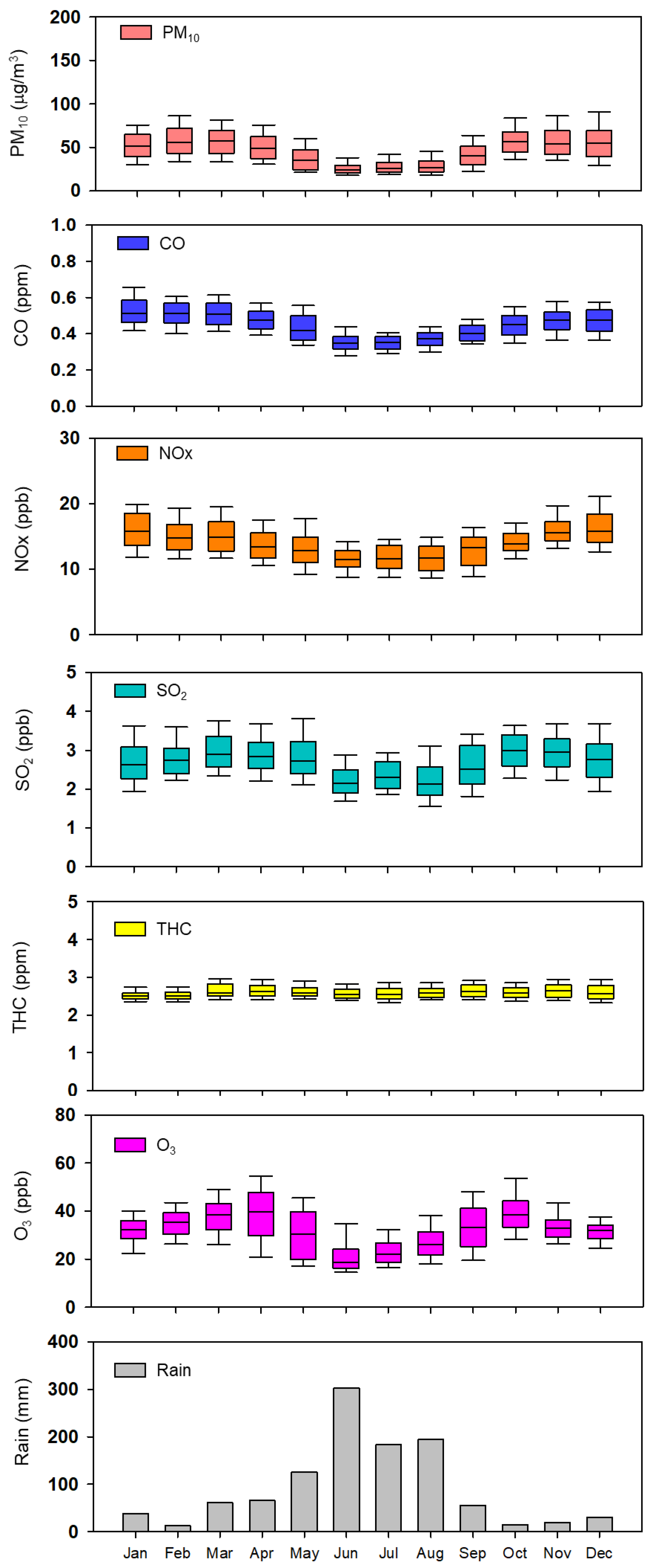
3.1. Criteria Air Pollutant Concentrations

Figure 2 shows the meteorological parameters and criteria for hourly pollutant variation. The hourly PM₁₀ average concentrations are 42 to 55 μg m⁻³ and the maximum concentration occurs from 08:00 to 09:00 (8 a.m.–9 a.m.) to 17:00, with the absolute maximum at 14:00. The hourly NOx average concentrations are 11.2 to 17.7 ppb, with the lowest values from 07:00 (7 a.m.) and between 13:00 and 14:00.

The SO₂ average hourly concentrations are 2.4–3.3 ppb and the greatest concentration occurs from 07:00 (7 a.m.), with the maximum from 09:00 to 10:00. The NMHC and THC average hourly concentrations are 0.14–0.22 and2.35–2.89 ppm, respectively. The O₃ average hourly concentrations are 19–52 ppb, and these are greatest from 07:00 (7 a.m.), with the highest values at 13:00. The average hourly CO concentrations are 0.39–0.50 ppm, with the greatest concentrations from 06:00 to 08:00 (6 a.m.–8 a.m.) and low concentration (about 0.39 ppm) at noon.

The solar radiation intensity increases with the increase in mixing height and then the wind also increases the entrainment of the particulate matter. In addition, the sea breeze is from the coastal area, and passes the petrochemical industry to associate with the SO₂ content of the air passing into the area. Furthermore, the O₃ formation relates to the intensity of solar radiation that leads to the development of mixing height at the boundary layer.

Figure 3 shows the variation in average monthly concentrations of PM₁₀, CO, NOx, SO₂, THC and O₃. Except for non-methane hydrocarbons, the average concentrations for these parameters are low from June to August (summertime is the rainy season and the prevailing monsoon is from the southwest). Average PM₁₀ concentrations in winter are 56 μg m⁻³, which is twice the level for summer. The average O₃ concentration in winter is 33 ppb, which is 40% higher than the value for summer.

The average NOx concentration in winter is 15.8 ppb, which is 1.4 times higher than the value for summer. The average SO₂ concentration in winter is 2.8 ppb, which is 1.2 times higher than the value for summer (2.28 ppb). The average NMHC/THC concentration in winter is 0.19/2.56 ppm, which is 10% more than the value for summer. The concentrations of criteria air pollutants are greater in winter than in summer.

Figure S1 shows the yearly variation in the average concentrations of PM₁₀, CO, NOx, SO₂, THC and O₃ for 2016–2020. The annual average concentrations of PM₁₀ are 40–52 μg m⁻³, for SO₂they are 2.4–3.0 ppb, for NOx they are 12–17 ppb, for THC they are 2.5–2.7 ppm, for CO they are 0.40–0.48 and for O₃they are 30–33 ppb. The PM₁₀, SO₂, THC and CO concentrations are lowest for 2020.There is a high PM concentration at D2 (61 μg m⁻³), possibly because there is entrainment of sand and dust from the river bed and low PM concentration at Sites D6 and D7 (40 μg m⁻³), which are located in the agricultural area, and because there is low traffic loading (shown in

Table 1. Variation in criteria air pollutant concentration for different years and locations.

Compounds	PM10	SO2	NOx	O3	THC	CO
	μg m−3	ppb	ppb	ppb	ppm	ppm
2016 (n = 366)	44.53 ± 5.84	3.02 ± 0.38	13.53 ± 1.93	30.23 ± 1.43	2.53 ± 0.11	0.44 ± 0.05
2017 (n = 365)	51.54 ± 8.47	2.77 ± 0.24	15.77 ± 1.24	32.11 ± 1.99	2.72 ± 0.11	0.44 ± 0.05
2018 (n = 365)	49.53 ± 8.00	2.63 ± 0.23	12.31 ± 1.72	33.35 ± 2.49	2.61 ± 0.38	0.43 ± 0.02
2019 (n = 365)	45.82 ± 7.85	2.71 ± 0.11	14.12 ± 0.91	33.03 ± 2.70	2.64 ± 0.40	0.48 ± 0.01
2020 (n = 366)	39.96 ± 6.27	2.39 ± 0.11	14.14 ± 1.45	31.39 ± 2.24	2.51 ± 0.31	0.40 ± 0.01
D1(n = 1827)	51.79 ± 4.40	2.80 ± 0.23	13.74 ± 1.34	31.31 ± 2.17	2.72 ± 0.16	0.44 ± 0.04
D2 (n = 1827)	60.98 ± 9.34	2.78 ± 0.20	13.69 ± 1.30	30.06 ± 0.85	2.80 ± 0.15	0.45 ± 0.02
D3 (n = 1827)	50.49 ± 5.24	2.79 ± 0.30	13.69 ± 1.31	33.50 ± 2.69	2.40 ± 0.18	0.42 ± 0.04
D4 (n = 1827)	47.70 ± 5.72	2.35 ± 0.20	17.50 ± 1.29	30.27 ± 1.14	2.69 ± 0.26	0.40 ± 0.05
D5 (n = 1827)	42.78 ± 5.12	2.83 ± 0.35	14.24 ± 1.34	30.54 ± 1.24	2.93 ± 0.18	0.43 ± 0.03
D6 (n = 1827)	39.76 ± 4.55	2.83 ± 0.46	12.77 ± 1.50	35.17 ± 0.84	2.29 ± 0.26	0.41 ± 0.04
D7 (n = 1827)	39.99 ± 8.16	2.70 ± 0.29	14.09 ± 1.30	30.70 ± 0.88	2.40 ± 0.32	0.46 ± 0.04
D8 (n = 1827)	43.78 ± 2.86	2.78 ± 0.38	14.62 ± 1.09	31.23 ± 1.76	2.73 ± 0.23	0.47 ± 0.04
D9 (n = 1827)	42.19 ± 3.15	2.64 ± 0.28	12.65 ± 1.73	33.35 ± 2.69	2.36 ± 0.24	0.47 ± 0.05
D10 (n = 1827)	43.31 ± 4.93	2.52 ± 0.22	12.79 ± 1.34	34.10 ± 2.47	2.69 ± 0.15	0.45 ± 0.03

).

Between 2016 and 2020, the average PM₁₀ concentration is high for 2017 (average concentration 52 μg m⁻³) and low for 2020 (average concentration 40 μg m⁻³).There is a high PM₁₀ at D2 and a low PM₁₀ value at D6.

From 2016 to 2020, the O₃ abundance is high for 2018 (average concentration 33 ppb) and low for 2016 (average concentration 30 ppb). O₃ levels are high near the downwind petrochemical complex district at D6, D9 and D10.

From 2016 to 2020, the NO_x abundance is high for 2017 (average concentration 15.7 ppb) and low for 2018 (average concentration 12.3 ppb). The NO₂ (17.5 ppb) is high at D4, which is located near a highway. The highway is probably the main source of pollution.

From 2016 to 2020, the SO₂ abundance is high for 2016 (average concentration 3.0 ppb) and low for 2020 (average concentration 2.4 ppb). The concentration of SO₂ (2.3–3.5 ppb) is high at D6, and the SO₂ concentration is at D4, with a value of 2.2–2.6 ppb.

From 2016 to 2020, the NMHC/THC abundance is high for 2016 (average concentration 0.21/2.53 ppm) and low for 2020 (average concentration 0.16/2.51 ppm). The NMHC/THC concentration is high (0.24–0.27/2.64–3.10 ppm) at D5 and low at D6 (0.05–0.22/2.37–2.95 ppm).

The development of mixing height increases with the average wind speed. After sunrise, the temperature increases and humidity decreases, as solar radiation increases.

There is a high correlation between CO and NOx, NMHC and THC, so these pollutants probably come from combustion sources. SOx emissions are not particularly significant compared to other pollutants, so they are probably emitted from various sources. Ozone is the primary form of the secondary pollutants from atmospheric reactions, so it is negatively correlated with CO, NOx, NMHC and THC. Except for PM₁₀, and O₃, mixing height and wind speed are negatively correlated with CO, NOx and hydrocarbons, possibly because high winds decrease the pollutant concentrations and entrain dust into the atmosphere (shown in Table S2).

The intensity of solar radiation is negatively correlated with relative humidity and positively correlated with temperature and mixing height. Solar radiation is also related to ozone concentration, particularly between 10:00 and16:00.

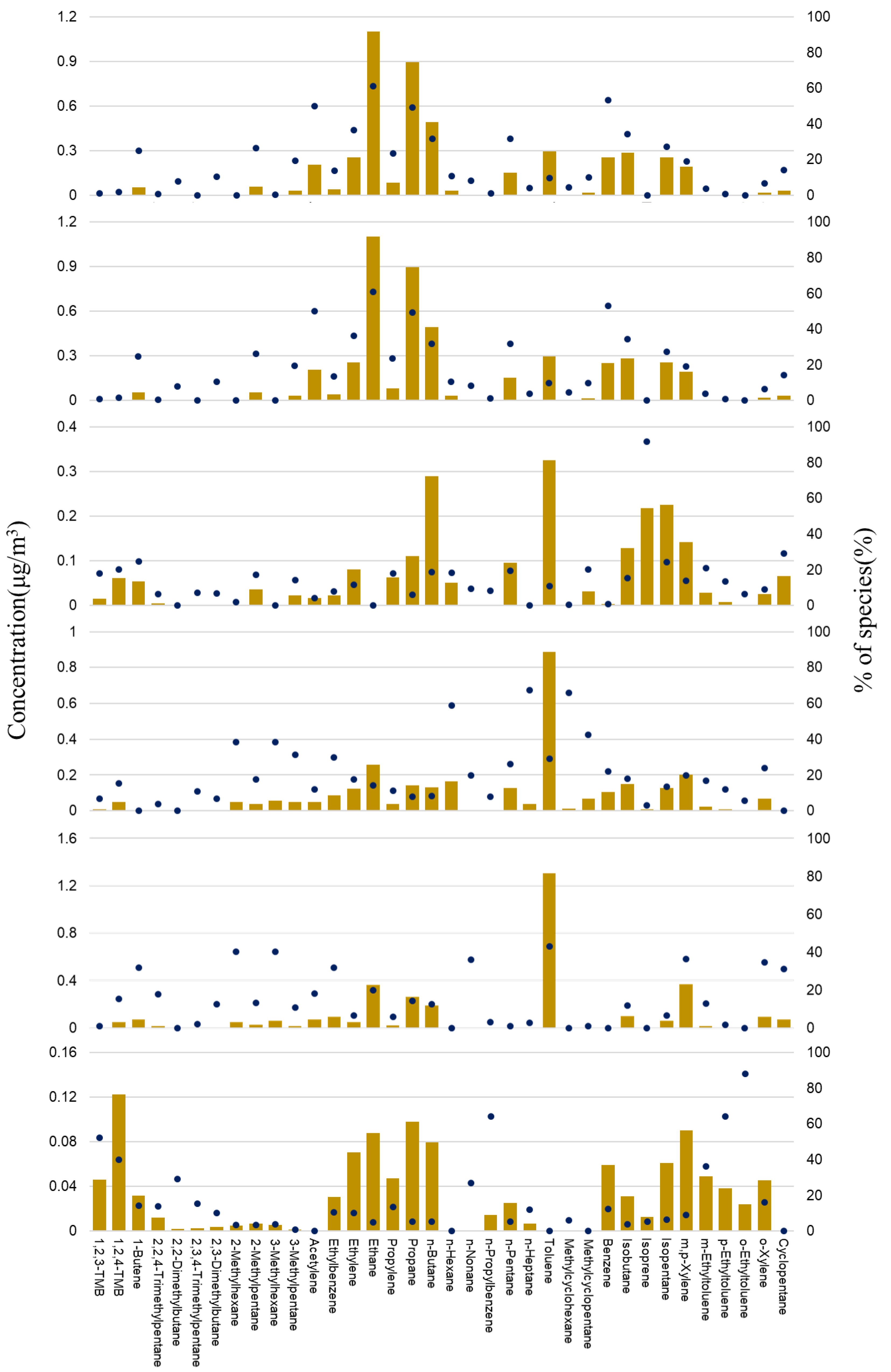
3.2. VOC Concentrations

Figure 4 shows the TVOC concentration and variation in species grouping for VOCs. Annual total VOC concentrations are 7.74–10.1 ppb for 2016–2020, of which 56–60% is alkanes, 14–15% is alkenes, 20–22% is aromatics and 5.2–6.8% is alkynes.

The predominant VOC concentration from 2016 to 2020 is shown in

Table 2. Major VOC species concentration (ppb) for 2016–2020.

Compounds	2016	2017	2018	2019	2020
	n = 366	n = 365	n = 365	n = 365	n = 366
Ethane	1.56 ± 0.95	1.56 ± 0.93	1.53 ± 0.88	1.64 ± 0.93	1.51 ± 0.90
Toluene	1.34 ± 0.87	1.22 ± 0.77	1.02 ± 0.64	0.98 ± 0.60	0.85 ± 0.53
Propane	1.26 ± 0.65	1.24 ± 0.81	1.12 ± 0.58	1.12 ± 0.60	1.06 ± 0.59
n-Butane	0.81 ± 0.34	0.77 ± 0.31	0.72 ± 0.30	0.71 ± 0.30	0.67 ± 0.27
Ethylene	0.80 ± 0.55	0.76 ± 0.35	0.70 ± 0.30	0.73 ± 0.38	0.66 ± 0.33
Acetylene	0.67 ± 0.32	0.56 ± 0.34	0.50 ± 0.28	0.50 ± 0.24	0.41 ± 0.23
Isobutane	0.49 ± 0.20	0.42 ± 0.18	0.36 ± 0.15	0.38 ± 0.17	0.36 ± 0.15
Isopentane	0.43 ± 0.16	0.43 ± 0.17	0.37 ± 0.15	0.35 ± 0.13	0.32 ± 0.13
Propene	0.37 ± 0.37	0.37 ± 0.30	0.28 ± 0.35	0.23 ± 0.18	0.26 ± 0.23
m,p-Xylene	0.25 ± 0.12	0.28 ± 0.14	0.24 ± 0.12	0.23 ± 0.12	0.25 ± 0.18
Benzene	0.25 ± 0.14	0.25 ± 0.15	0.20 ± 0.12	0.18 ± 0.12	0.16 ± 0.10
Pentane	0.24 ± 0.09	0.22 ± 0.09	0.18 ± 0.08	0.17 ± 0.08	0.17 ± 0.07
n-Hexane	0.16 ± 0.10	0.15 ± 0.09	0.12 ± 0.06	0.11 ± 0.09	0.09 ± 0.08
1-Butene	0.16 ± 0.05	0.17 ± 0.04	0.14 ± 0.09	0.10 ± 0.04	0.11 ± 0.04
2-Methylpentane	0.12 ± 0.05	0.10 ± 0.04	0.07 ± 0.03	0.07 ± 0.03	0.06 ± 0.03
Isoprene	0.10 ± 0.11	0.08 ± 0.08	0.09 ± 0.09	0.08 ± 0.07	0.09 ± 0.08
1,2,4-Trimethylbenzene	0.09 ± 0.04	0.10 ± 0.05	0.09 ± 0.04	0.08 ± 0.04	0.06 ± 0.04
3-Methylpentane	0.09 ± 0.04	0.07 ± 0.03	0.06 ± 0.03	0.06 ± 0.03	0.05 ± 0.02
o-Xylene	0.08 ± 0.05	0.09 ± 0.05	0.07 ± 0.04	0.07 ± 0.04	0.07 ± 0.07
Ethylbenzene	0.08 ± 0.05	0.10 ± 0.05	0.08 ± 0.05	0.08 ± 0.04	0.07 ± 0.05
Others	0.70	0.72	0.56	0.51	0.45
Alkanes	5.66 ± 2.45	5.44 ± 2.33	4.91 ± 2.18	4.96 ± 2.24	4.63 ± 2.05
Alkenes	1.49 ± 0.86	1.46 ± 0.62	1.23 ± 0.48	1.16 ± 0.55	1.45 ± 0.50
Aromatics	2.24 ± 1.25	2.19 ± 1.19	1.84 ± 0.99	1.72 ± 0.92	1.55 ± 0.88
Alkynes	0.67 ± 0.32	0.56 ± 0.34	0.50 ± 0.28	0.50 ± 0.24	0.41 ± 0.23
Sum	10.06	9.68	8.52	8.36	7.73

. The results of this study show that the principal VOCs are ethane (1.51–1.64 ppb), toluene (0.85–1.34 ppb), propane(1.06–1.26 ppb), n-butane(0.67–0.81 ppb), ethylene(0.66–0.80 ppb) and acetylene (0.41–0.67 ppb). The annual average concentration of these compounds is more than 0.50 ppb. The production of oil and natural gas and biomass burning are the two most significant sources of ethane and propane emissions into the atmosphere [57,58]. This is consistent with the results of a previous study, which found that the petrochemical industry releases olefins-unsaturated aliphatic hydrocarbons (such as ethylene, propylene and butadiene) and aromatic-unsaturated cyclic hydrocarbons (such as benzene, toluene, and xylenes) into the atmosphere [59].

Traffic-related VOCs are the primary anthropogenic sources of ambient VOCs and ozone precursors in metropolitan urban environments, so VOC emissions from sources of gasoline aromatics significantly impact the release of toluene and benzene into the environment [60].

The fuel-based emission factors for volatile organic compounds (VOCs) are 0.8 to 2.6 g kg⁻¹ and alkanes are the dominant components (ethylene, acetylene, propylene and isobutene from diesel vehicles) (>80%) [61]. This is consistent with the results of previous studies, which showed that tailpipe emissions of VOCs typically comprise a mixture of unburned fuel (most significantly, toluene, xylenes and a range of C4–C10 alkanes) and products from partial combustion (ethene, formaldehyde, acetaldehyde and propene) [62]. Studies in the UK showed that the dominant VOCs that are released from evaporative fuel loss are C6 and C5 alkanes, xylenes, ethanol, butane, propane and toluene and smaller amounts of a range of other alkanes and alkenes [62].

The average annual benzene concentration is 0.16–0.25 ppb. Toluene concentrations decrease from 1.34 ± 0.87 to 0.85 ± 0.53 ppb from 2016 to 2020 (Figure S2). Olefin (ethylene, propene and butadiene) and aromatic species (benzene, toluene and xylene) are produced by the Sixth Naphtha Cracker petrochemical industry.

The toluene to benzene ratio is 5.2 ± 0.2 (4.8–5.4 from 2016 to 2020) and the high T/B ratio shows that vehicular emissions contribute to hydrocarbon emissions. The T/B ratio is high at D4 (7.71) and D2 (6.39) because of VOCs from motor vehicles. The T/B ratio is low at D6, D9 and D10 (3.71–3.95) and the emissions from petrochemical facilities contain significant amounts of VOCs. The toluene-to-xylene ratio is highest at D4 (4.69) and lowest at D6 (1.81), possibly due to the effect of direct emission sources at D6.

Less reactive VOC species accumulate during the day, but highly reactive VOC species are reduced by photochemical processes during the day. The toluene-to-benzene (T/B) ratio is used as an indicator of traffic emissions [63,64,65,66] so the T/B ratio in the exhausts of moving vehicles may be close to one. An increase in this ratio indicates industrial emissions [67]. The values range from 1.5 to 3.0 [64,65,68,69] and the differences are most likely due to different vehicle types and fuel compositions in different geographical locations. A lower T/B ratio in the ambient air may be due to air mass transportation and degradation and a higher T/B ratio may be due to recent vehicle emissions or typical emission sources.

Xylene is more reactive than benzene, which has an atmospheric lifetime of 12.5 days compared to 7.8 h for xylene, so a low xylene/benzene (X/B) ratio explains air mass ageing [70,71,72]. The (m + p)-xylene to ethylbenzene ((m + p)/E)-ratio is also an indicator of the photochemical age of the air mass [70,73].

The respective concentrations of m,p-xylene and ethylbenzene are 0.22 to 0.37 ppb and 0.07 to 0.10 ppb. From 2016 to 2020, the xylene-to-ethylbenzene ratio is 2.8 to 4.6. This figure is attributed to hydrocarbon sources: primarily refineries and exhausts [70]. Sampling point D4 was next to a highway, so automobiles are the most likely cause of the high BTEX content at this station (shown as Figure S3), which is consistent with the results of a previous study [74].

Figure 5 shows the variation in the hourly concentration of benzene, toluene, ethylbenzene and xylene. Benzene average hourly concentrations are high at 07:00 a.m., decrease until 13:00 to 15:00, and then increase again. Benzene concentration is high between January and April and October and December and low between May and September. During the wet season, ambient benzene levels decrease. Toluene average hourly concentrations are high at 07:00 a.m., decrease until 13:00 to 15:00, and then increase again. Ethylbenzene average hourly concentrations are high at 07:00 a.m., decrease until 13:00, and then increase again.

Hourly O₃ concentration increases with the decrease in NOx, butane, acetylene, isopentane, propene and toluene, especially in the time during 10:00–17:00 (shown in Figure S4). The anthropogenic activities (such as mobile emission, industrial emission, etc.), can be the important sources of NOx and VOCs leading to the O₃ formation after sunrise. The correlation coefficient analysis indicates that the O₃ reveals a high negative correlation coefficient with the NOx, NMHC, toluene, isopentane and butane (shown as Table S3). In addition, the isoprene increases with the increase in O₃, which indicates that the isoprene emission is attributable to the vegetation. The Pearson’s statistics show that benzene has a correlation with toluene, ethylbenzene and xylene.

Figure 6 shows the average monthly concentration for major VOC species. Average VOC concentrations are 5.7–12 ppb for 2016–2020. VOC concentrations are low in the summer (from June to August, when the concentration ranges from 5.7 to 5.9 ppb) and high in winter (from December to February, with a concentration of 11–12 ppb). For different VOC groups, the results show that concentration decreases in the following order: alkanes (52–63%), aromatics (18–24%), alkenes (11–22%) and alkynes (4.7–7.1%). The concentrations of alkanes, aromatics and alkynes are high in winter and low in summer, but the concentration of alkenes is only slightly lower in the summer. The average total concentration of VOCs is 11.5 ppb in winter, which is approximately twice the concentration in summer (5.8 ppb).

The highest concentration of TVOCs is observed at 07:00. The concentration decreases until 13:00, and then increases until 07:00 the following day. VOC concentrations are 7.65 ± 0.79 to 11.16 ± 1.21 ppb. VOC concentrations are high at D4 and D8 (average concentrations exceed 10 ppb) and low at D1, D10 and D5 (average concentrations of less than 8.0 ppb).

3.3. Ozone Formation Potential (Hourly Variations)

The ozone formation potentials for VOCs are shown in

Table 3. Ozone formation potential for VOCs (μg m⁻³) from 2016 to 2020.

Compound	2016	2017	2018	2019	2020
	n = 366	n = 365	n = 365	n = 365	n = 366
Toluene	24.26	22.12	18.48	17.83	15.36
m,p-Xylene	8.51	9.46	8.27	7.81	8.43
Ethylene	8.30	7.89	7.20	7.52	6.79
Propene	7.37	7.54	5.64	4.71	5.28
1,2,4-Trimethylbenzene	4.04	4.49	3.93	3.32	2.73
Isoprene	3.09	2.48	2.72	2.33	2.72
1-Butene	3.51	3.88	3.22	2.21	2.43
o-Xylene	2.81	2.93	2.39	2.29	2.38
n-Butane	2.22	2.12	1.98	1.95	1.85
Isopentane	1.86	1.82	1.59	1.50	1.39
1,2,3-Trimethylbenzene	1.79	1.77	1.68	1.39	1.23
Isobutane	1.43	1.22	1.07	1.11	1.05
3-Ethyltoluene	1.62	1.62	1.40	1.21	1.00
Ethylbenzene	1.11	1.27	1.07	1.01	0.96
Propane	1.11	1.10	0.99	0.99	0.93
Pentane	0.92	0.86	0.70	0.67	0.66
Cyclopentane	0.47	0.46	0.41	0.45	0.70
Ethane	0.54	0.54	0.53	0.56	0.52
trans-2-Butene	1.13	1.02	0.67	0.50	0.44
1,3,5-Trimethylbenzene	0.67	0.87	0.66	0.56	0.41
Acetylene	0.68	0.57	0.51	0.51	0.41
Benzene	0.57	0.58	0.47	0.41	0.37
Others	6.28	6.35	4.85	4.18	3.33
Alkanes	12.85	12.16	10.40	10.17	9.41
Alkenes	24.31	23.90	20.11	17.69	18.08
Aromatics	46.45	46.34	39.39	36.63	33.47
Alkynes	0.68	0.57	0.51	0.51	0.41
Sum	84.29	82.97	70.41	65.00	61.37

. These results show that toluene (15.4–24.3 μg-O₃ m⁻³), m,p-xylene (7.81–9.46 μg-O₃ m⁻³), ethylene (6.79–8.30 μg-O₃ m⁻³), propene (4.71–7.54 μg-O₃ m⁻³), 1,2,4-trimethylbenzene (2.73–4.49 μg-O₃ m⁻³), isoprene (2.33–3.09 μg-O₃ m⁻³), 1-butene (2.21–3.88 μg-O₃ m⁻³), o-xylene (2.29–2.93 μg-O₃ m⁻³), n-butane (1.85–2.22 μg-O₃ m⁻³) and isopentane (1.39–1.86 μg-O₃ m⁻³) are the major contributing species to the potential for zone formation. The OFP decreases from 84 μg-O₃ m⁻³ (2016) to 61 μg-O₃ m⁻³ (2020).

The OFP average hourly abundance is high from 06:00 to 7:00 a.m. The concentration then decreases from 13:00 to 15:00, and increases again. At 13:00, the hourly average for OFP is lowest, because the intensity of solar radiation is highest, which increases atmospheric photochemical reactions. After sunrise at 06:00, the intensity of solar radiation increases, is greatest at 11:00–13:00 (2.2–2.3 MJ m⁻²), and decreases after sunset.

Ethylene, propene, butane, toluene and xylenes how the same variations in concentration. However, the OFP for isoprene is different to that for other species, so isoprene is emitted from different sources to those of other VOC species. Isoprene is present in plant or vegetable emissions.

The ozone formation potential for VOCs increases from 14:00 to 7:00 the next day, with a peak value of126.2 μg-O₃ m⁻³. The value then decreases to 45.7 μg-O₃ m⁻³ at 13:00 (shown in Figure S5).

The maximum value for winter to spring (highest peak in March (94.4 μg-O₃ m⁻³)) and the minimum value during summer are determined using the monthly OFP for VOCs (rainy season from June to August) (shown in Figure S6).

The OPF for VOCs is of 56.4 ± 8.0–96.1 ± 13.4μg-O₃ m⁻³. The OFP is high in D4 (96.1 ± 13.4 μg-O₃ m⁻³) and D8 (92.3 ± 16.8 μg-O₃ m⁻³) (average OFPs are higher than 90 μg-O₃ m⁻³) and VOC concentrations in D1 and D10 are low (average OFPs are less than 60 μg-O₃ m⁻³) (shown in Figure S7).

There are few works which have looked at the VOCs from agricultural emission that lead to the lack of VOC emission from agricultural activities (vegetable, animal manure, cropland and pasture, etc.). In the Metro Vancouver area, the agriculture was proportional to about 2.7% VOC emission, while 78% VOC was emitted from industry and 20% from natural vegetation [75]. Generally, volatile and semi volatile biogenic VOC fractions including oxygenated VOCs, isoprene, monoterpenes, and sesquiterpenes were determined in the atmosphere of mid-European agricultural and natural plants [76]. In Yunlin, the biogenic VOCs (BVOCs) amounted to 10,500 tons/year and most of them were isoprene, and mono-terpenes in 2021 [46]. The high proportion of biogenic VOCs contributed to the total VOCs in Yunlin county, and therefore, the species of BVOCs are important for determining their OFP. However, the lack of specie compositions of BVOCs can be a limitation for the development of ambient ozone control strategies in the future.

3.3.1. Air Mass Transport—Back Trajectory Analysis

The air mass trajectory analysis for summer and winter is shown in Figure 7. In summer, 25% of the air mass comes from southern inland Taiwan, moving to Yunlin, 40% from the southwest and through the South China Sea, 15% from the west, circling in the coastal area of Southern China, 7.5% from the north through the Taiwan Strait and 15% from the south and inland Southern Taiwan, to Yunlin. A total of 10% of the air mass comes from the south, moving to Yunlin, and 12.5% comes from other directions, so air pollutants are decreased by the rainy season in summer.

The air masses were 34% greater in winter, with high pollution levels in the air from the west of Eastern China via the East China Sea and from inland Northern Taiwan to Yunlin. A total of 9.4% of the air mass comes from the coast of Mainland China, 37.5% from the northeast, through the East China Sea to Yunlin, and 9.4% from North Taiwan (East China Sea).

3.3.2. Contribution of Emission Sources

Data for the emission of TEDs (Taiwan emission data system-10) shows that the pollutant emission of PM_2.5, SO_x, NO_x, CO and NMHC was 3053, 8898, 25,768, 31,825 and 17,928 ton yr⁻¹, respectively, in 2016. A total of 36% of PM_2.5 emissions are from construction and road dust, 25% from industrial facilities, 25% from mobile sources and 6% from off-road vehicles. A total of 65% of SO₂ emissions are from stationary sources and 33% from mobile sources; 58% of NO_x emissions are from stationary sources, 35% from mobile sources, and 6% from off-road vehicles. A total of 56% of CO emissions are from stationary sources and 37% from mobile sources; 34% of NMHC emissions are from stationary sources, 22% from mobile sources, 30% from commercial sources and 13% from the construction industry.

3.3.3. VOC Sources for PMF Results

The VOC emission sources have apositive matrix factor (PMF) and conduct as determined by EPA PMF, version 5. The uncertainty of PMF is shown in Table S4, and results are shown in Figure 8.

Factor 1 accounts for 28.7% of the VOC contribution and contains high levels of ethane (23.1%), propane (18.8%), n-butane (10.4%), isobutene (5.95%), benzene (5.32%) and toluene (6.32%). The process in the Sixth Naphtha Cracker releases ethane, propane, and n-butane. The production of natural gas and oil, the burning of biofuels and the burning of biomass fuel produce a significant amount of non-methane hydrocarbons (NMHC) such as ethane in the atmosphere [77]. Propane, n-butane, i-butane and butenes are the main components of LPG evaporative emissions [78], so fuel leakage and evaporation from an industrial area, especially natural gas or LPG, contribute to this type of pollution.

Factor 2 explains 13.1% of the VOC sources. The major VOCs are n-butane (16.9%), propane (14.5%), toluene (10.5%), isopentane (9.42%) and its derivatives (such as 2,2,4-trimethylpentane). The main components of gasoline in this context are isopentane, n-butane, toluene and 2,2,4-trimethylpentane [79].

Concentrations of ethylene, isopentane, ethane and toluene and ethane and propane are higher in VOC emissions from gasoline vehicles and LNG-fueled vehicles. Methyl tert-butyl ether, 2,2,4-trimethylpentane,2,3,4-trimethylpentane, 3-methylpentane and methylcyclopentane are potential VOC tracers for gasoline vaporization [80].

Factor 3 accounts for 12.9% of the VOC contribution, followed by toluene (15.2%), n-butane (13.5%), isoprene (10.2%), isopentane (10.6%), m,p-xylene (6.64%) and propane (5.18%). Gasoline contains a large amount of isopentane and C4 and C5 alkanes [81,82,83]. A study by Sun et al. [84] showed the isopentane and n-pentane are indicators for gasoline evaporation. A high composition of isoprene is mostly due to phytoncide that is released from plants, so this factor is attributed to biogenic emissions.

Factor 4 explains 18.4% of the VOC contribution. Toluene (29.0%), ethane (8.37%) and m,p-xylene (6.59%) are dominant in factor 4. The benzene-toluene-xylene mixture is used for back mixing of petrol to increase octane ratings. Petrochemical production is the source of toluene and xylene. Ethane is also an element of fossil fuel emissions [85] and is used for ethylene production [86], so this factor is explained by the use of solvents in the petrochemical industry.

Factor 5 explains 20.3% of the VOC contribution. Toluene (38.6%), ethane (10.7%), m,p-xylene (10.9%), propane (7.73%), n-butane(5.70%), (ethylene, 2-methylhexane, 3-methylhexane, 1-butene, o-xylene) also contribute. Toluene, xylene, ethane, propane and n-butane are products of petrochemical refineries [87], so this factor is attributed to emissions from the petrochemical industry.

Factor 6 explains 6.4% of the VOC contribution. 1,2,4-trimethylbenzene (11.1%), 1,2,3-TMB (4.16%), ethane(7.92%), propane(8.81%), n-butane (7.170%), benzene (5.34%), m,p-xylene(8.15%), isopentane (5.48%) also contribute. The emissions come from fuel combustion.

The PMF analysis and VOCs emission sources for this study show that the primary sources of VOCs are industrial facilities, the petrochemical industry, solvent application, fuel combustion, motor vehicle exhaust emissions and evaporation and vegetable emissions. Diesel engines have a higher combustion efficiency because most of the higher hydrocarbons are burned, so a characteristic source profile for diesel exhaust contains ethene (26%), propene (14%) and acetylene (11%) [81,82,83,84,85,86,87,88]. Diesel engines are demonstrated to have a higher combustion efficiency [89] but there are no significant differences in the profiles of different types of diesel vehicles. Ethene, propene, acetylene, benzene, 1,2,3-trimethylbenzene and 1-butene are the dominant NMHCs.

In Taiwan, ozone pollution associated with a VOC-sensitive regime was decreased from 72 to 55%, corresponding to the period 2007 to 2020 [90]. Therefore, VOC reduction is important for ambient ozone pollutants. However, the NOx reduction is also concerned in this, following the control strategies for VOC emission in recent years.

4. Conclusions

Average PM₁₀, SOx, and O₃ hourly concentrations increase with the development of mixing height and an increase in wind speed. These results show that PM₁₀, SO₂, and O₃ levels increase when the mixing height increases and solar radiation levels increase, and NOx and hydrocarbon concentrations decrease as the concentration of O₃ and the solar radiation intensity increase. For the average monthly concentration, pollutant concentrations are low from May to September, due to the monsoon and rainy season. Pollutant concentrations increase from October to the following April. VOC concentrations are 7.65–11.2 ppb. VOC concentrations are high at D4 and D8, and low VOC concentrations of 20–30% are present at D1, D10 and D5. Total VOC concentrations decrease with the development of mixing height after sunrise. Alkanes and aromatics contribute a high fraction of VOCs. The concentrations of toluene, benzene, xylene, ethylene and isopentane are highest at 07:00, because human activity increases at this time. Isoprene concentrations depend on solar radiation and are mainly emitted from the vegetation. The ozone formation potential for VOC species show that toluene, xylene, ethylene, propene, 1,2,4-trimethylbenzene, Isoprene and 1-butene contribute 73–75% of OFP and that the OFP decreases from 84 μg-O₃ m⁻³ in 2016 to 61 μg-O₃ m⁻³ in 2020.

References

1. USEPA. Health Effects Notebook for Hazardous Air Pollutants. 2013. Available online: http://www.epa.gov/ttn/atw/hlthef/hapindex.html (accessed on 1 June 2022).
2. Guo, H.; Lee, S.C.; Chan, L.Y.; Li, W.M. Risk assessment of exposure to volatile organic compounds in different indoor environments. Environ. Res. 2004, 94, 57–66. [Google Scholar] [CrossRef] [PubMed]
3. Chang, E.E.; Wang, W.C.; Zeng, L.X.; Chiang, H.L. Health risk assessment of exposure to selected volatile organic compounds emitted from an integrated iron and steel plant. Inhal. Toxicol. 2010, 22, 117–125. [Google Scholar] [CrossRef] [PubMed]
4. Yang, W.B.; Chen, W.H.; Yuan, C.S.; Yang, J.C.; Zhao, Q.L. Comparative assessments of VOC emission rates and associated health risks from wastewater treatment processes. J. Environ. Monit. 2012, 14, 2464–2474. [Google Scholar] [CrossRef] [PubMed]
5. Ryerson, T.B.; Trainer, M.; Angevine, W.M.; Brock, C.A.; Dissly, R.W.; Fehsenfeld, F.C.; Frost, G.J.; Goldan, P.D.; Holloway, J.S.; Hubler, G.; et al. Effect of petrochemical industrial emissions of reactive alkenes and NOx on tropospheric ozone formation in Houston, Texas. J. Geophys. Res.-Atmos. 2003, 108, 4249. [Google Scholar] [CrossRef]
6. Elbir, T.; Cetin, B.; Cetin, E.; Bayram, A.; Odabasi, M. Characterization of Volatile Organic Compounds (VOCs) and Their Sources in the Air of Izmir, Turkey. Environ. Monit. Assess. 2007, 133, 149–160. [Google Scholar] [CrossRef]
7. Wang, H.; Lou, S.; Huang, C.; Qiao, L.; Tang, X.; Chen, C.; Zeng, L.; Wang, Q.; Zhou, M.; Lu, S.; et al. Source Profiles of Volatile Organic Compounds from Biomass Burning in Yangtze River Delta, China. Aerosol Air Qual. Res. 2014, 14, 818–828. [Google Scholar] [CrossRef]
8. Drozd, G.T.; Zhao, Y.; Saliba, G.; Frodin, B.; Maddox, C.; Weber, R.J.; Chang, M.C.O.; Maldonado, H.; Sardar, S.; Robinson, A.L.; et al. Time Resolved Measurements of Speciated Tailpipe Emissions from Motor Vehicles: Trends with Emission Control Technology, Cold Start Effects, and Speciation. Environ. Sci. Technol. 2016, 50, 13592–13599. [Google Scholar] [CrossRef]
9. Cheng, J.; Zhang, Y.; Wang, T.; Xu, H.; Norris, P.; Pan, W.P. Emission of volatile organic compounds (VOCs) during coal combustion at different heating rates. Fuel 2018, 225, 554–562. [Google Scholar] [CrossRef]
10. Liu, H.; Man, H.; Tschantz, M.; Wu, Y.; He, K.; Hao, J. VOC from vehicular evaporation emissions: Status and control strategy. Environ. Sci. Technol. 2015, 49, 14424–14431. [Google Scholar] [CrossRef]
11. Yuan, B.; Shao, M.; Lu, S.H.; Wang, B. Source profiles of volatile organic compounds associated with solvent use in Beijing, China. Atmos. Environ. 2010, 44, 1919–1926. [Google Scholar] [CrossRef]
12. Fuentes, J.D.; Lerdau, M.; Atkinson, R.; Baldocchi, D.; Bottenheim, J.W.; Ciccioli, P.; Lamb, B.; Geron, C.; Gu, L.; Guenther, A.; et al. Biogenic hydrocarbons in the atmospheric boundary layer: A review. Bull. Am. Meteorol. Soc. 2000, 81, 1537–1575. [Google Scholar] [CrossRef]
13. Mo, Z.; Shao, M.; Lu, S.; Niu, H.; Zhou, M.; Sun, J. Characterization of nonmethane hydrocarbons and their sources in an industrialized coastal city, Yangtze River Delta, China. Sci. Total Environ. 2017, 593–594, 641–653. [Google Scholar] [CrossRef] [PubMed]
14. Mo, Z.; Lu, S.; Shao, M. Volatile organic compound (VOC) emissions and health risk assessment in paint and coatings industry in the Yangtze River Delta, China. Environ. Pollut. 2021, 269, 115740. [Google Scholar] [CrossRef] [PubMed]
15. de Gouw, J.A.; Middlebrook, A.M.; Warneke, C.; Goldan, P.D.; Kuster, W.C.; Roberts, J.M.; Fehsenfeld, F.C.; Worsnop, D.R.; Canagaratna, M.R.; Pszenny, A.A.P.; et al. Budget of organic carbon in a polluted atmosphere: Results from the New England Air Quality Study in 2002. J. Geophys. Res. 2005, 110, D16305. [Google Scholar] [CrossRef]
16. Wang, M.; Qin, W.; Chen, W.; Zhang, L.; Zhang, Y.; Zhang, X.; Xie, X. Seasonal variability of VOCs in Nanjing, Yangtze River delta: Implications for emission sources and photochemistry. Atmos. Environ. 2020, 223, 117254. [Google Scholar] [CrossRef]
17. Liu, P.W.G.; Yao, Y.C.; Tsai, J.H.; Hsu, Y.C.; Chang, L.P.; Chang, K.H. Source impacts by volatile organic compounds in an industrial city of southern. Taiwan Sci. Total Environ. 2008, 398, 154–163. [Google Scholar] [CrossRef] [PubMed]
18. Liu, C.C.; Chen, W.H.; Yuan, C.S.; Lin, C.S. Multivariate analysis of effects of diurnal temperature and seasonal humidity variations by tropical savanna climate on the emissions of anthropogenic volatile organic compounds. Sci. Total Environ. 2014, 470, 311–323. [Google Scholar] [CrossRef]
19. Kalabokas, P.D.; Hatzianestis, J.; Bartzis, J.G.; Papagiannakopoulos, P. Atmospheric concentrations of saturated and aromatic hydrocarbons around a Greek oil refinery. Atmos. Environ. 2001, 35, 2545–2555. [Google Scholar] [CrossRef]
20. Guenther, A.; Karl, T.; Harley, P.; Wiedinmyer, C.; Palmer, P.I.; Geron, C. Estimates of global terrestrial isoprene emissions using MEGAN (model of emissions of gases and aerosols from nature). Atmos. Chem. Phys. 2006, 6, 3181–3210. [Google Scholar] [CrossRef]
21. Cetin, E.; Odabasi, M.; Seyfioglu, R. Ambient volatile organic compound (VOC) concentrations around a petrochemical complex and a petroleum refinery. Sci. Total. Environ. 2003, 312, 103–112. [Google Scholar] [CrossRef]
22. Chang, K.H.; Chen, T.F.; Huang, H.C. Estimation of biogenic volatile organic compounds emissions in subtropical island e Taiwan. Sci. Total Environ. 2005, 346, 184–199. [Google Scholar] [CrossRef] [PubMed]
23. Tiwari, V.; Hanai, Y.; Masunaga, S. Ambient levels of volatile organic compounds in the vicinity of petrochemical industrial area of Yokohama, Japan. Air Qual. Atmos. Health 2010, 3, 65–75. [Google Scholar] [CrossRef] [PubMed]
24. Rao, P.-S.; Ansari, M.-F.; Gavane, A.-G.; Pandit, V.-I.; Nema, P.; Devotta, S. Seasonal variation of toxic benzene emissions in petroleum refinery. Environ. Monit. Assess. 2007, 28, 323–328. [Google Scholar] [CrossRef] [PubMed]
25. Pandya, G.H.; Gavane, A.G.; Bhanarkar, A.D.; Kondawar, V.K. Concentrations of volatile organic compounds (VOCs) at an oil refinery. Int. J. Environ. Stud. 2006, 63, 337–351. [Google Scholar] [CrossRef]
26. Baltrėnas, P.; Baltrėnaitė, E.; Šerevičienė, V.; Pereira, P. Atmospheric BTEX concentrations in the vicinity of the crude oil refinery of the Baltic region. Environ. Monit. Assess. 2011, 182, 115–127. [Google Scholar] [CrossRef] [PubMed]
27. Dumanoglu, Y.; Kara, M.; Altiok, H.; Odabasi, M.; Elbir, T.; Bayram, A. Spatial and seasonal variation and source apportionment of volatile organic compounds (VOCs) in a heavily industrialized region. Atmos. Environ. 2014, 98, 168–178. [Google Scholar] [CrossRef]
28. Song, Y.; Dai, W.; Shao, M.; Liu, Y.; Lu, S.; Kuster, W.; Goldan, P. Comparison of receptor models for source apportionment of volatile organic compounds in Beijing, China. Environ. Pollut. 2008, 156, 174–183. [Google Scholar] [CrossRef]
29. Volkamer, R.; Jimenez, J.L.; San Martini, F.; Dzepina, K.; Zhang, Q.; Salcedo, D.; Molina, L.T.; Worsnop, D.R.; Molina, M.J. Secondary organic aerosol formation from anthropogenic air pollution: Rapid and higher than expected. Geophys. Res. Lett. 2006, 33, L17811. [Google Scholar] [CrossRef]
30. Gariazzo, C.; Pelliccioni, A.; Di Filippo, P.; Sallusti, F.; Cecinato, A. Monitoring and analysis of volatile organic compounds around an oil refinery. Water Air Soil Pollut. 2005, 167, 17–38. [Google Scholar] [CrossRef]
31. Hoyt, D.; Raun, L.H. Measured and estimated benzene and volatile organic carbon (VOC) emissions at a major U.S. refinery/chemical plant: Comparison and prioritization. J. Air Waste Manag. Assoc. 2015, 65, 1020–1031. [Google Scholar] [CrossRef]
32. Lin, T.Y.; Sree, U.; Tseng, S.H.; Chiu, K.H.; Wu, C.H.; Lo, J.G. Volatile organic compound concentrations in ambient air of Kaohsiung petroleum refinery in Taiwan. Atmos. Environ. 2004, 38, 4111–4122. [Google Scholar] [CrossRef]
33. Sonibare, J.A.; Akeredolu, F.A.; Obanijesu, E.O.O.; Adebiyi, F.M. Contribution of volatile organic compounds to Nigeria’s Airshed by petroleum refineries. Pet. Sci. Technol. 2007, 25, 503–516. [Google Scholar] [CrossRef]
34. Wei, W.; Lv, Z.; Yang, G.; Cheng, S.; Li, Y.; Wang, L. VOCs emission rate estimate for complicated industrial area source using an inverse-dispersion calculation method: A case study on a petroleum refinery in Northern China. Environ. Pollut. 2016, 218, 681–688. [Google Scholar] [CrossRef] [PubMed]
35. Hajizadeh, Y.; Teiri, H.; Nazmara, S.; Parseh, I. Environmental and biological monitoring of exposures to VOCs in a petrochemical complex in Iran. Environ. Sci. Pollut. Res. 2018, 25, 6656–6667. [Google Scholar] [CrossRef] [PubMed]
36. Han, D.; Gao, S.; Fu, Q.; Cheng, J.; Chen, X.; Xu, H.; Liang, S.; Zhou, Y.; Ma, Y. Do volatile organic compounds (VOCs) emitted from petrochemical industries affect regional PM2.5? Atmos. Res. 2018, 209, 123–130. [Google Scholar] [CrossRef]
37. Yuan, Z.; Zhong, L.; Lau, A.K.H.; Yu, J.Z.; Louie, P.K.K. Volatile organic compounds in the Pearl River Delta: Identification of source regions and recommendations for emission-oriented monitoring strategies. Atmos. Environ. 2013, 76, 162–172. [Google Scholar] [CrossRef]
38. Mo, Z.; Shao, M.; Lu, S.; Qu, H.; Zhou, M.; Sun, J.; Gou, B. Process-specific emission characteristics of volatile organic compounds (VOCs) from petrochemical facilities in the Yangtze River Delta, China. Sci. Total Environ. 2015, 533, 422–431. [Google Scholar] [CrossRef]
39. Wang, Q.; Li, S.; Dong, M.; Li, W.; Gao, X.; Ye, R.; Zhang, D. VOCs emission characteristics and priority control analysis based on VOCs emission inventories and ozone formation potentials in Zhoushan. Atmos. Environ. 2018, 182, 234–241. [Google Scholar] [CrossRef]
40. Feng, Y.; Xiao, A.; Jia, R.; Zhu, S.; Gao, S.; Li, B.; Shi, N.; Zou, B. Emission characteristics and associated assessment of volatile organic compounds from process units in a refinery. Environ. Pollut. 2020, 265, 115026. [Google Scholar] [CrossRef]
41. Lyu, X.; Guo, H.; Wang, Y.; Zhang, F.; Nie, K.; Dang, J.; Liang, Z.; Dong, S.; Zeren, Y.; Zhou, B.; et al. Hazardous volatile organic compounds in ambient air of China. Chemosphere 2020, 246, 125731. [Google Scholar] [CrossRef]
42. Ramirez, M.I.; Arevalo, A.P.; Sotomayor, S.; Bailon-Moscoso, N. Contamination by oil crude extraction-refinement and their effects on human health. Environ. Pollut. 2017, 231, 415–425. [Google Scholar] [CrossRef] [PubMed]
43. Dai, L.; Meng, J.; Zhao, X.; Li, Q.; Shi, B.; Wu, M.; Zhang, Q.; Su, G.; Hu, J.; Shu, X. High-spatial-resolution VOCs emission from the petrochemical industries and its differential regional effect on soil in typical economic zones of China. Sci. Total Environ. 2022, 827, 154318. [Google Scholar] [CrossRef] [PubMed]
44. International Agency for Research on Cancer (IARC). IARC Monographs on the Identification of Carcinogenic Hazards to Human, World Health Organization. Available online: https://monographs.iarc.who.int/ (accessed on 7 September 2022).
45. Liang, Y.; Liu, X.; Wu, F.; Guo, Y.; Fan, X.; Xiao, H. The year-round variations of VOC mixing ratios and their sources in Kuytun City (northwestern China), near oilfields. Atmos. Pollut. Res. 2020, 11, 1513–1523. [Google Scholar] [CrossRef]
46. Taiwan Environmental Protection Agency (TEPA). Taiwan Air Pollutants Emission Data System. 2023. Available online: https://teds.epa.gov.tw/Introduction.aspx (accessed on 1 April 2023).
47. Russell, A.; Milford, J.; Bergin, M.S.; McBride, S.; McNair, L.; Yang, Y.; Stockwell, W.; Croes, B. Urban Ozone Control and Atmospheric Reactivity of Organic Gases. Science 1995, 269, 491–495. [Google Scholar] [CrossRef] [PubMed]
48. Carter, W.P.L. Updated Maximum Incremental Reactivity Scale and Hydrocarbon in Reactivities for Regulatory Applications; Prepared for California Air Resources Board Contract 07-339; University of California: Riverside, CA, USA, 2009. [Google Scholar]
49. Fang, X.; Saito, T.; Park, S.; Li, S.; Yokouchi, Y.; Prinn, R.G. Performance of Back-Trajectory Statistical Methods and Inverse Modeling Method in Locating Emission Sources. ACS Earth Space Chem. 2018, 2, 843–851. [Google Scholar] [CrossRef]
50. Leuchner, M.; Rappenglück, B. VOC source–receptor relationships in Houston during TexAQS-II. Atmos. Environ. 2010, 44, 4056–4067. [Google Scholar] [CrossRef]
51. Paatero, P. Least Squares Formulation of Robust, Non-Negative Factor Analysis. Chemom. Intell. Lab. Syst. 1997, 37, 23–35. [Google Scholar] [CrossRef]
52. Paatero, P.; Tapper, U. Positive matrix factorization: A non-negative factor model with optimal utilization of error estimates of data values. Environmetrics 1994, 5, 111–126. [Google Scholar] [CrossRef]
53. Kuo, C.P.; Liao, H.T.; Chou, C.C.; Wu, C.F. Source apportionment of particulate matter and selected volatile organic compounds with multiple time resolution data. Sci. Total Environ. 2014, 472, 880–887. [Google Scholar] [CrossRef]
54. Reff, A.; Eberly, S.I.; Bhave, P.V. Receptor modeling of ambient particulate matter data using positive matrix factorization: Review of existing methods. J. Air Waste Manag. 2007, 57, 146–154. [Google Scholar] [CrossRef]
55. Poirot, R.L.; Wishinski, P.R.; Hopke, P.K.; Polisar, A.V. Comparative Application of Multiple Receptor Methods to Identify Aerosol Sources in Northern Vermont. Environ. Sci. Technol. 2001, 35, 4622–4636. [Google Scholar] [CrossRef] [PubMed]
56. Buzcu, B.; Fraser, M.P. Source identification and apportionment of volatile organic compounds in Houston, TX. Atmos. Environ. 2006, 40, 2385–2400. [Google Scholar] [CrossRef]
57. Helmig, D.; Rossabi, S.; Hueber, J.; Tans, P.; Montzka, S.A.; Masarie, K.; Thoning, K.; Plass-Duelmer, C.; Claude, A.; Carpenter, L.J.; et al. Reversal of global atmospheric ethane and propane trends largely due to US oil and natural gas production. Nat. Geosci. 2016, 9, 490–495. [Google Scholar] [CrossRef]
58. Angot, H.; Davel, C.; Wiedinmyer, C.; Pétron, G.; Chopra, J.; Hueber, J.; Blanchard, B.; Bourgeois, I.; Vimont, I.; Montzka, S.A.; et al. Temporary pause in the growth of atmospheric ethane and propane in 2015–2018. Atmos. Chem. Phys. 2021, 21, 15153–15170. [Google Scholar] [CrossRef]
59. Benchaita, T. Greenhouse Gas Emissions from New Petrochemical Plants; No. IDB-TN-562; Inter-American Development Bank: Washington, DC, USA, 2013. [Google Scholar]
60. Zhang, M.; Ge, Y.; Li, J.; Wang, X.; Tan, J.; Hao, L.; Xu, H.; Hao, C.; Wang, J.; Qian, L. Effects of ethanol and aromatic contents of fuel on the non-regulated exhaust emissions and their ozone forming potential of E10-fueled China-6 compliant vehicles. Atmos. Environ. 2021, 264, 118688. [Google Scholar] [CrossRef]
61. Li, C.; Cui, M.; Zheng, J.; Chen, Y.; Liu, J.; Ou, J.; Tang, M.; Sha, Q.; Yu, F.; Liao, S.; et al. Variability in real-world emissions and fuel consumption by diesel construction vehicles and policy implications. Sci. Total Environ. 2021, 786, 147256. [Google Scholar] [CrossRef]
62. NAEI. UK National Atmospheric Emissions Inventory. 2020. Available online: http://naei.beis.gov.uk/ (accessed on 20 December 2022).
63. Miller, L.; Lemke, L.D.; Xu, X.; Molaroni, S.M.; You, H.; Wheeler, A.J.; Booza, J.; Grgicak-Mannion, A.; Krajenta, R.; Graniero, P.; et al. Intra-urban correlation and spatial variability of air toxics across an international airshed in Detroit, Michigan (USA) and Windsor, Ontario (Canada). Atmos. Environ. 2010, 44, 1162–1174. [Google Scholar] [CrossRef]
64. Hoque, R.R.; Khillare, P.S.; Agarwal, T.; Shridhar, V.; Balachandran, S. Spatial and temporal variation of BTEX in the urban atmosphere of Delhi, India. Sci. Total Environ. 2008, 392, 30–40. [Google Scholar] [CrossRef]
65. Barletta, B.; Meinardi, S.; Rowland, F.S.; Chan, C.Y.; Wang, X.; Zou, S.; Chan, L.Y.; Blake, D.R. Volatile organic compounds in 43 Chinese cities. Atmos. Environ. 2005, 39, 5979–5990. [Google Scholar] [CrossRef]
66. Buczynska, A.J.; Krata, A.; Stranger, M.; Godoi, A.F.L.; Kontozova-Deutsch, V.; Bencs, L.; Naveau, I.; Roekens, E.; Grieken, R.V. Atmospheric BTEX-concentrations in an area with intensive street traffic. Atmos. Environ. 2009, 43, 311–318. [Google Scholar] [CrossRef]
67. Gelencser, A.; Siszler, K.; Hlavay, J. Toluene-benzene concentration ratio as a tool for characterizing the distance from vehicular emission sources. Environ. Sci. Technol. 1997, 31, 2869–2872. [Google Scholar] [CrossRef]
68. Chiang, P.C.; Chiang, Y.C.; Chang, E.E.; Chang, S.C. Characterizations of hazardous air pollutants emitted from motor vehicles. Environ. Toxicol. Chem. 1996, 56, 85–104. [Google Scholar] [CrossRef]
69. Liu, J.; Mu, Y.; Zhang, Y.; Zhang, Z.; Wang, X.; Liu, Y.; Sun, Z. Atmospheric levels of BTEX compounds during the 2008 Olympic Games in the urban area of Beijing. Sci. Total Environ. 2009, 408, 109–116. [Google Scholar] [CrossRef]
70. Nelson, P.F.; Quigley, S.M. The m,p-xylenes: Ethylbenzene ratio. A technique for estimating hydrocarbon age in ambient atmospheres. Atmos. Environ. 1983, 17, 659–662. [Google Scholar] [CrossRef]
71. Prinn, R.; Cunnold, D.; Rasmussen, R.; Simmonds, P.; Alyea, F.; Crawford, A.; Fraser, P.; Rosen, R. Atmospheric trends in methylchloroform and the global average for the hydroxyl radical. Science 1987, 238, 945–950. [Google Scholar] [CrossRef] [PubMed]
72. Na, K.; Kim, Y.P. Seasonal characteristics of ambient volatile organic compounds in Seoul, Korea. Atmos. Environ. 2001, 35, 2603–2614. [Google Scholar] [CrossRef]
73. Zhang, J.; Wang, T.; Chameides, W.L.; Cardelino, C.; Blake, D.R.; Streets, D.G. Source characteristics of volatile organic compounds during high ozone episodes in Hong Kong, Southern China. Atmos. Chem. Phys. 2008, 8, 4983–4996. [Google Scholar] [CrossRef]
74. Abbasi, F.; Pasalari, H.; Delgado-Saborit, J.M.; Rafiee, A.; Abbasi, A.; Hoseini, M. Characterization and risk assessment of BTEX in ambient air of a Middle Eastern City. Process Saf. Environ. Prot. 2020, 139, 98–105. [Google Scholar] [CrossRef]
75. Roumeliotis, T.; Guenther, A.; Durward, D.; Pourbafrani, H. Relative Impact of Volatile Organic Compound Emissions from Agriculture on Air Quality of Urban Centres. In Food and Fisheries; Governments of Canada and British Columbia, British Columbia Ministry of Agriculture: Abbotsford, BC, Canada, 2021. [Google Scholar]
76. König, G.; Brunda, M.; Puxbaum, H.; Hewitt, C.N.; Duckham, S.C.; Rudolph, J. Relative contribution of oxygenated hydrocarbons to the total biogenic VOC emissions of selected mid-European agricultural and natural plant species. Atmos. Environ. 1995, 29, 861–874. [Google Scholar] [CrossRef]
77. Li, M.; Pozzer, A.; Lelieveld, J.; Williams, J. Global atmospheric ethane, propane and methane trends(2006–2016). Earth Syst. Sci. Data 2021, 2021, 1–30. [Google Scholar] [CrossRef]
78. Kumar, A.; Sinha, V.; Shabin, M.; Hakkim, H.; Bonsang, B.; Gros, V. Non-methane hydrocarbon (NMHC) fingerprints of major urban and agricultural emission sources for use in source apportionment studies. Atmos. Chem. Phys. 2020, 20, 12133–12152. [Google Scholar] [CrossRef]
79. Gentner, D.R.; Harley, R.A.; Miller, A.M.; Goldstein, A.H. Diurnal and Seasonal Variability of Gasoline-Related Volatile Organic Compound Emissions in Riverside, California. Environ. Sci. Technol. 2009, 43, 4247–4252. [Google Scholar] [CrossRef] [PubMed]
80. Song, C.; Liu, Y.; Sun, L.; Zhang, Q.; Mao, H. Emissions of volatile organic compounds (VOCs) from gasoline- and liquified natural gas (LNG)-fueled vehicles in tunnel studies. Atmos. Environ. 2020, 234, 117626. [Google Scholar] [CrossRef]
81. Liu, Y.; Shao, M.; Fu, L.; Lu, S.; Zeng, L.; Tang, D. Source profiles of volatile organic compounds (VOCs) measured in China: Part I. Atmos. Environ. 2008, 42, 6247–6260. [Google Scholar] [CrossRef]
82. Zhang, Y.; Wang, X.; Barletta, B.; Simpson, I.J.; Blake, D.R.; Fu, X.; Zhang, Z.; He, Q.; Liu, T.; Zhao, X.; et al. Source attributions of hazardous aromatic hydrocarbons in urban, suburban and rural areas in the Pearl River Delta (PRD) region. J. Hazard. Mater. 2013, 250–251, 403–411. [Google Scholar] [CrossRef] [PubMed]
83. Li, B.; Ho, S.S.H.; Xue, Y.; Huang, Y.; Wang, L.; Cheng, Y.; Dai, W.; Zhong, H.; Cao, J.; Lee, S. Characterizations of volatile organic compounds (VOCs) from vehicular emissions at roadside environment: The first comprehensive study in Northwestern China. Atmos. Environ. 2017, 161, 1–12. [Google Scholar] [CrossRef]
84. Sun, J.; Wu, F.; Hu, B.; Tang, G.; Zhang, J.; Wang, Y. VOC characteristics, emissions and contributions to SOA formation during hazy episodes. Atmos. Environ. 2016, 141, 560–570. [Google Scholar] [CrossRef]
85. Dalsøren, S.B.; Myhre, G.; Hodnebrog, Ø.; Myhre, C.L.; Stohl, A.; Pisso, I.; Schwietzke, S.; Höglund-Isaksson, L.; Helmig, D.; Reimann, S.; et al. Discrepancy between simulated and observed ethane and propane levels explained by underestimated fossil emissions. Nat. Geosci. 2018, 11, 178–184. [Google Scholar] [CrossRef]
86. Ghanta, M.; Fahey, D.; Subramaniam, B. Environmental impacts of ethylene production from diverse feedstocks and energy sources. Appl. Petrochem. Res. 2014, 4, 167–179. [Google Scholar] [CrossRef]
87. Zhang, Z.; Wang, H.; Chen, D.; Li, Q.; Thai, P.; Gong, D.; Li, Y.; Zhang, C.; Gu, Y.; Zhou, L.; et al. Emission characteristics of volatile organic compounds and their secondary organic aerosol formation potentials from a petroleum refinery in Pearl River Delta, China. Sci. Total Environ. 2017, 584–585, 1162–1174. [Google Scholar] [CrossRef]
88. Schauer, J.J.; Kleeman, M.J.; Cass, G.R.; Simoneit, B.R. Measurement of emissions from air pollution sources, 2. C1 through C30 organic compounds from medium duty diesel trucks. Environ. Sci. Technol. 1999, 33, 1578–1587. [Google Scholar] [CrossRef]
89. Reiter, M.S.; Kockelman, K.M. The problem of cold starts: A closer look at mobile source emissions levels. Transp. Res. D Transp. Environ. 2016, 43, 123–132. [Google Scholar] [CrossRef]
90. Chen, T.F.; Tsai, C.Y.; Chen, C.H.; Chang, K.H. Effect of long-range transport from changing emission on ozone-NOx-VOC sensitivity: Implication of control strategy to improve ozone. J. Innov. Technol. 2021, 3, 39–49. [Google Scholar] [CrossRef]
Figure 1. VOC monitoring stations and major emission sources in Yunlin.
Atmosphere 14 00803 g001
Figure 2. Average variation in hourly concentration for meteorological variation (wind speed, temperature, humidity, mixing height) and criteria pollutants.
Atmosphere 14 00803 g002
Figure 3. Monthly variations in the concentration of criteria air pollutants and rainfall.
Atmosphere 14 00803 g003
Figure 4. Average hourly concentration variation of VOC groups.
Atmosphere 14 00803 g004
Figure 5. Variation in average hourly concentration of VOC species.
Atmosphere 14 00803 g005
Figure 6. Monthly variation in TVOC concentration.
Atmosphere 14 00803 g006
Figure 7. Back-trajectory analysis of air mass using the HYSPLIT model: (a) summer cases (b) winter cases.
Atmosphere 14 00803 g007
Figure 8. VOC emission sources are determined using PMF. (Bar chart indicates the VOC concentration and circle point indicates the percentage for different factors).
Atmosphere 14 00803 g008