Article

A Metamodel-Based Optimization of Physical Parameters of High Resolution NWP ICON-LAM over Southern Italy

by
Davide Cinquegrana
*,
Alessandra Lucia Zollo
,
Myriam Montesarchio
and
Edoardo Bucchignani
Meteorology Lab, Centro Italiano Ricerche Aerospaziali (CIRA), Via Maiorise, 81043 Capua, CE, Italy
*
Author to whom correspondence should be addressed.
Atmosphere 2023, 14(5), 788; https://doi.org/10.3390/atmos14050788
Submission received: 22 February 2023 / Revised: 5 April 2023 / Accepted: 21 April 2023 / Published: 26 April 2023
(This article belongs to the Special Issue Numerical Analysis in Atmospheric Research)

Abstract

:
This work represents a first step in the definition of a framework aimed at finding, by means of efficient global optimization based on metamodels, an optimal configuration of physical parameters for the ICON (ICOsahedral Nonhydrostatic) Limited Area Mode at high resolution (about 1.1 km) over Southern Italy, to be used for operational runs. The objective of the optimization is to reduce the distance between observed meteorological variables and modeled data. This distance is measured by an opportunely designed objective function. This work represents a preparatory step, since the input parameters considered are only a reduced number with respect to the huge amount of parameters potentially involved. First, domain size sensitivity was performed to choose the optimal domain. Then, the optimization was conducted by means of an Efficient Global Optimization algorithm relying on a Gaussian-based metamodel. The four parameters considered control the heat transfer in the turbulent layer, the laminar resistance and the snow vertical velocity. They were optimized over a week in November 2018, a period characterized by extreme events in the region considered. The results demonstrated the effectiveness of the proposed approach, reducing the distance from observed data, and the method can be considered promising from the perspective taking into account a larger set of physical parameters, and validation over a wider time-window.

1. Introduction—Background and Motivations

Limited Area Models in weather forecasts allow very accurate simulations on small scales, thanks to their higher grid resolution, if compared to Global Models (GMs). Generally, the physical parameters of local models, which are often inherited by GM at a coarser horizontal resolution, need to be re-calibrated over the specific domain of interest, in order to consider new orographic features, which may be quite different from coarser ones. The geographical configurations, and the fact that high resolution allows new phenomena to be simulated, need to be taken into account.
Re-calibration is often performed by ’experts’ within the judgement of a parameters tuning campaign, even if, in the last decade, increasing attention has been oriented to automatic calibration. However, this technique is still limited, due to its huge CPU requirements, as highlighted in the work conducted by Duan et al. [1], where the authors emphasize the difficulties of this approach. They refer to the large number of physical parameters involved (a ’curse of dimension’ problem), which makes the optimization hard to apply in practice, and to the fact that it requires a multi-objective approach, due to the meteorological variables to be monitored. In order to reduce the CPU request when performing an automatic calibration, metamodels are replacing the numerical weather solver response, as shown in the work by Neelin et al. [2], where the authors investigated the sensitivity to physical parameters of a climate GM and conducted parameters optimization based on a multi-quadratic regression model. Bellprat et al. [3] tried to reduce the bias of Regional Climate Models by optimizing eight parameters by means of the same metamodel proposed in [2]. Duan et al. [1] performed a calibration of the WRF (Weather Research & Forecasting) model over the Beijing area, tuning nine parameters with an adaptive surrogate modeling-based optimization. Recently, Vouduri et al. [4] obtained only slight model performance gain, but underlined that an objective calibration methodology could have a significant impact on the future development of NWP models for re-calibration after major model changes (e.g., different horizontal and/or vertical resolutions).
With this view in mind, a crucial task is the selection of model parameters having a functional relationship to the forecast quantities to be optimized. A successive step is the definition of the optimization target, i.e., the objective function, which, consequently, defines the nature of the optimization problem. Although huge effort has been expended, currently there is poor agreement among authors [2] on the definition of scalar metrics [3,5,6] or on the cost functions useful for parameter optimization. For example, Gleckeler [6] highlighted the risk that a single index can be misleading, since the complex behavior of the variables involved could show opposite trends and interact in a non-linear way, underlining that the development of suitable metrics is quite a complex process. In the present work, three meteorological variables were considered in the calibration process, with the aim of enhancing their representation in a satisfactory manner. Even if the process requires model calibration conducted via a multi-objective approach, it is known that this approach further increases the complexity of model calibration. Hence, the approach followed here is based on a single-value objective function that aggregates with a scalar weight. This linear weights combination allows effective reduction of the computational cost, though it can introduce several other advantages and disadvantages [7]. In this way, we can transform the optimization problem into a single objective using a surrogate-based optimization technique, aiming to find a solution that represents the best compromise for each variable, and imitating, or at least approximating, a Pareto optimal point [8].
The aim of this work was to provide a contribution to the definition of a suitable high-resolution model configuration for ICON-LAM over southern-Italy, where the numerical model parameters are tuned with automated model calibration. This calibration is based on a metamodel that measures the distance from the observed data of different physical variables (e.g., temperature at surface level and precipitation over 24 h) and the numerical model predictions. A single object optimization in the parameter space is set to find the best parameter configurations that minimize the distance from measured data. These methods replace the expert knowledge approach that can be considered a manual, trial and error approach with intrinsic limitations. The expert judgement approach often starts from a sensitivity analysis of the target function to model parameter changes. This approach, according to the number of parameters involved, does not take into account mutual interactions between parameter changes, but considers perturbations of assigned reference levels for one parameter at a time. Approaches like the one presented in this work are, instead, based on full interaction of the parameters involved. The aim of a well-fitted n-dimensional metamodel is to describe the multimodal landscape of the target function and to predict its behavior in unknown data points, supporting the optimization algorithm in finding the global optimum, and avoiding local minima. On the other hand, a surrogate model-assisted optimization contributes to saving CPU-time if compared to algorithms that feed optimum search directly with results from numerical models (ICON in our case). With this approach, we aimed to set up an automated process that is able to find optimal values of tuning parameters controlling physical parameterization schemes, enhancing the model configuration. Furthermore, starting from the results obtained from the first optimization campaign, a new one could be performed, involving additional parameters alongside the data obtained, in the framework of a refinement chain based on successive optimizations.
ICON (ICOsahedral Nonhydrostatic) is a joint project between the Deutscher Wetterdienst (DWD) and the Max Planck Institute for Meteorology (MPI-M) for the development of a unified global numerical weather prediction system [9]. ICON can also be run as a Limited Area Mode (ICON-LAM) and is replacing the COSMO (Consortium for Small-scale Modeling) model in climate and weather forecasting. A major source of uncertainty arises from the large number of unconstrained model parameters associated to the parameterization schemes. The selection of the parameters to be calibrated is a crucial task, since there are numerous parameters in the ICON-LAM configuration [9].
In order to fulfil the objective of the work, domain sensitivity and an automatic calibration of physical parameters were performed over a domain located in southern Italy. This aimed to contribute to the definition of a model configuration suitable for accurate weather forecasts over this area.
A first sensitivity analysis was performed with respect to the domain size, considering a reference domain and two additional domains that were respectively 50% and 100% larger (in both directions) than the original one. Then, an automatic calibration of four critical physical parameters was carried out starting from a model configuration previously defined by the authors (in a joint effort with the CMCC Foundation, Italy) for the whole Italian area, employing a different resolution (R2B10, about 2.5 km) [10]. The tuning was performed over the following parameters that were previously shown to play a significant role in determining model response: tkhmin (minimal diffusion coefficient for heat and moisture), tkmmin (minimal diffusion coefficient for momentum), rlam_heat (factor for laminar resistance for heat) and v0snow (factor for vertical velocity of snow).
Model evaluation was conducted against observational data provided by the SCIA dataset (ISPRA, Italy) [11]. Moreover, a comparison with forecasts provided by the COSMO model at 0.009° (about 1 km resolution) forced by the same driving data was performed, in order to highlight the differences between the performances of the two models. This paper is organized as follows. In Section 2, the model ICON-LAM is described, while the domain and the observational data are shown in Section 3. In Section 4 we describe the test cases under investigation and the SW/HW configuration. In Section 5.1 we describe how the results were post-processed to obtain the objective function F o b j (described in Section 5.2), which was minimized in the automatic calibration process, described in Section 5.3. In Section 6 we discuss the results related to the domain sensitivity, to the automatic calibration and to the validation of the optimized configurations over an independent dataset, i.e., a week in summer, 2019. Finally, Section 7 and Section 8 are devoted to a discussion of results and conclusions, respectively.

2. ICON-LAM: Model Description and Set Up

In 2018, the COSMO consortium started migrating from the COSMO-LM to the ICON-LAM (ICON Limited Area mode) as the operational model. ICON-LAM is characterized by exact local mass conservation and mass consistent tracer transport. The dynamical core is formulated on an icosahedral-triangular Arakawa C-grid. Time integration is performed with a two-time level predictor–corrector fully explicit scheme. Time splitting is applied between the dynamical core and tracer advection, physics parameterization and horizontal diffusion. Physics-dynamic coupling is performed at constant density ( ρ ), rather than pressure, since ρ is a prognostic variable, whereas pressure is only diagnosed for parametrization, hydrostatically integrated. The fast physics parametrization was inherited from the COSMO model, except for the saturation adjustment. The Cloud micro-physics scheme is an extended version of COSMO-EU, with modification of cloud–ice sedimentation. The turbulence scheme has undergone some revision from ICON to improve stability under extreme conditions. The TERRA land-surface scheme has also been extended with a multi-layer snow scheme and tile-based approach accounting for sub-grid scale land-cover variability. Slow physics were imported from the Integrated Forecast System (IFS). Since simulations are initialized with horizontally interpolated data, a tile “cold-start” approach has been employed, where each tile is initialized with the same cell averaged value, and the initial values with a guess from a run without tiles.
The optimization process performed in the present work starts from a configuration name list (here referred to as baseline), inherited from the work described in [10], where a suitable configuration for the whole Italian peninsula was defined, based on a reference defined at DWD (Germany) with some modifications suggested by the Israeli Meteorological Service (IMS, Israel). This reference configuration assumes that the shallow convection parameterization is active, whereas the parts treating deep- and mid-level convection are switched off. Moreover, a single moment cloud microphysics scheme and a diagnostic Kohler cloud cover scheme are employed. The parameters to be calibrated were selected after a long selection process carried out in the frame of the Priority Projects CALMO and CALMO-MAX of the COSMO Consortium [12], aimed at developing a method supporting an objective calibration of the input parameters of the COSMO model. This selection was a crucial task, since there are numerous parameters in the COSMO model indicatively related to sub-grid scale turbulence, surface layer parameterization, grid-scale clouds, precipitation, moist and shallow convection, radiation, soil scheme, etc. In particular, in [13], the most sensitive physical and numerical input parameters were identified for a domain similar to the one considered in the present work. It was found that the parameters with a relevant influence for a proper representation of temperature and precipitation are the heat resistance length of the laminar layer, the minimal diffusion coefficient for heat and momentum, and a factor controlling the vertical velocity of snow. Table 1 shows the four parameters explored in the automatic calibration, together with their variation ranges and reference values. The ranges were chosen in order to preserve physical significance. The parameters considered were associated with turbulence (tkhmin, tkmmin), surface layer parametrization (rlam_heat) and grid scale precipitation (v0snow). The following points are particularly relevant:
  • v0snow is the factor in the terminal velocity for snow and is used in the grid scale clouds and precipitation parametrization;
  • tkmmin is the scaling factor for minimum vertical diffusion coefficient (proportional to Richardson number, R i 2 / 3 ) for momentum;
  • tkhmin controls the minimum value for the turbulence coefficient (proportional to Richardson number, R i 2 / 3 ) for heat and moisture;
  • rlam_heat is a scaling factor of the laminar boundary layer for heat (scalars), with larger values corresponding to larger laminar resistance.
Table 1. Calibrated parameters: ranges, reference values and descriptions.
NameParametrizationMin.Max.BaselineDescription
v0snow [ - ]Microphysics103030Snow vertical velocity
tkhmin [ m 2 /s]Vertical turbulent diffusion0.12.00.5Heat diffusion coefficient
tkmmin [ m 2 /s]Vertical turbulent diffusion0.12.00.75Momentum diffusion coefficient
rlam_heat [ - ]Soil and vegetation processes0.0520.010.0Heat laminar resistance factor
The simulations were performed on the CIRA server ’Turing’, an HPC cluster, based on the RedHat Enterprise Linux v7.3 Operating System, equipped with 40 Intel Xeon E5-2697 nodes, for a total of 1440 cores, interconnected by means of an Intel Omni-Path network at 100 Gbit/s. The ICON release installed was the 2.6.4, compiled with Intel Parallel Studio 2020 XE update 4 with MPI intel libraries. Each simulation was run distributing the day/instance on 4 nodes, in order to meet internal queue policies. Each simulation employed about 4 h of elapsed time per day.

3. Domains and Observational Data

The computational domain of a regional climate or weather forecast model must be carefully selected for its specific application. In particular, domains sufficiently larger than the area of interest are needed for studies of sensitivity to internal forcing [14]. Goswami et al. [15] stated, for example, that along with initial conditions and resolution, the size of the domain significantly affects simulated quantities, such as total precipitation. Furthermore, they showed that, for both average and maximum precipitation, the dispersion in simulations, due to variations of the domain size, is much larger than the dispersion due to either initial conditions or grid spacing.
The limited area over which a model is integrated must be large enough to allow the full development of small-scale features [16] and to avoid side effects from lateral boundaries. On the other hand, a larger horizontal domain could include complex topographic areas, absent in the smaller, potentially affecting the extended domain with unexpected degradation [17].
In this study three domains of increasing size were considered (Figure 1), in order to select the one that performed better in terms of temperature and cumulative precipitation forecast over the considered period. The domains included the northern Campania and southern Lazio regions and were characterized by a spatial resolution of about 1.1 km, i.e., computational grid R2B11. Further details can be found in Table 2.
Model evaluation was conducted against both grid and in-situ station data provided by the SCIA-Ispra (National System for elaboration of Climate data) system. Specifically, over the domain considered, data from 28 stations are available for temperature and 48 for precipitation (Figure 2). Grid data (obtained through an interpolation process, already considered in a previous work [10]) are available over the whole domain on a regular grid at 5 km resolution for temperature and 10 km for precipitation. Furthermore, the outputs of ICON simulations were also compared with the results obtained with COSMO on a similar domain.

4. The Test Cases Considered

Following the work performed by the authors with COSMO on a similar domain [13], the week 19–25 November 2018, was selected for the test case for the optimization of the ICON-LAM model configuration, when a low-pressure system, coming from the Western Mediterranean, brought intense storms and gusts. The region analyzed is generally exposed to humid westerly winds and, consequently, high precipitation values are recorded, even along the coasts, of up to 1000 mm/year. In particular, the first part of the selected week was characterized by a low pressure system coming from the Western Mediterranean that ran over Sardinia first and then hit the south-central regions of Italy. Moreover, a second test case was conducted for the week 1–7 July 2019, in order to test the effectiveness of the optimized model configuration in a different season (summer) involving different weather regimes, since the relevance of many tuning parameters depends strongly on the meteorological conditions, and interactions with existing biases originating from other sources may vary with the season. This week was characterized by high temperatures, with the risk of heat waves in urban areas. It is very likely that if the two periods (a winter week and a summer week) were reversed the results would change, but this verification was beyond the purposes of the present work.
A computational grid R2B11, characterized by a very high resolution (about 1.1 km), was adopted. The time step was set equal to 12 s. Initial and boundary conditions were provided by the ECMWF IFS model at a spatial resolution of about 8.5 km. The boundary conditions were updated every 3 h. A series of 24 h forecasts was performed, restarting from interpolated IFS conditions on each day.

5. Methodology

In this section, the operations needed to associate the numerical ICON outputs with a useful scalar function, easily handled by the automatic calibration process, are described in the post-processing section. The design of a scalar function that can assess enhancement resulting from variation of the selected physical parameters from the baseline configuration, in terms of distance from reference data, was followed. Finally, the automatic calibration method is described in the last section.

5.1. Post-Processing of ICON Results

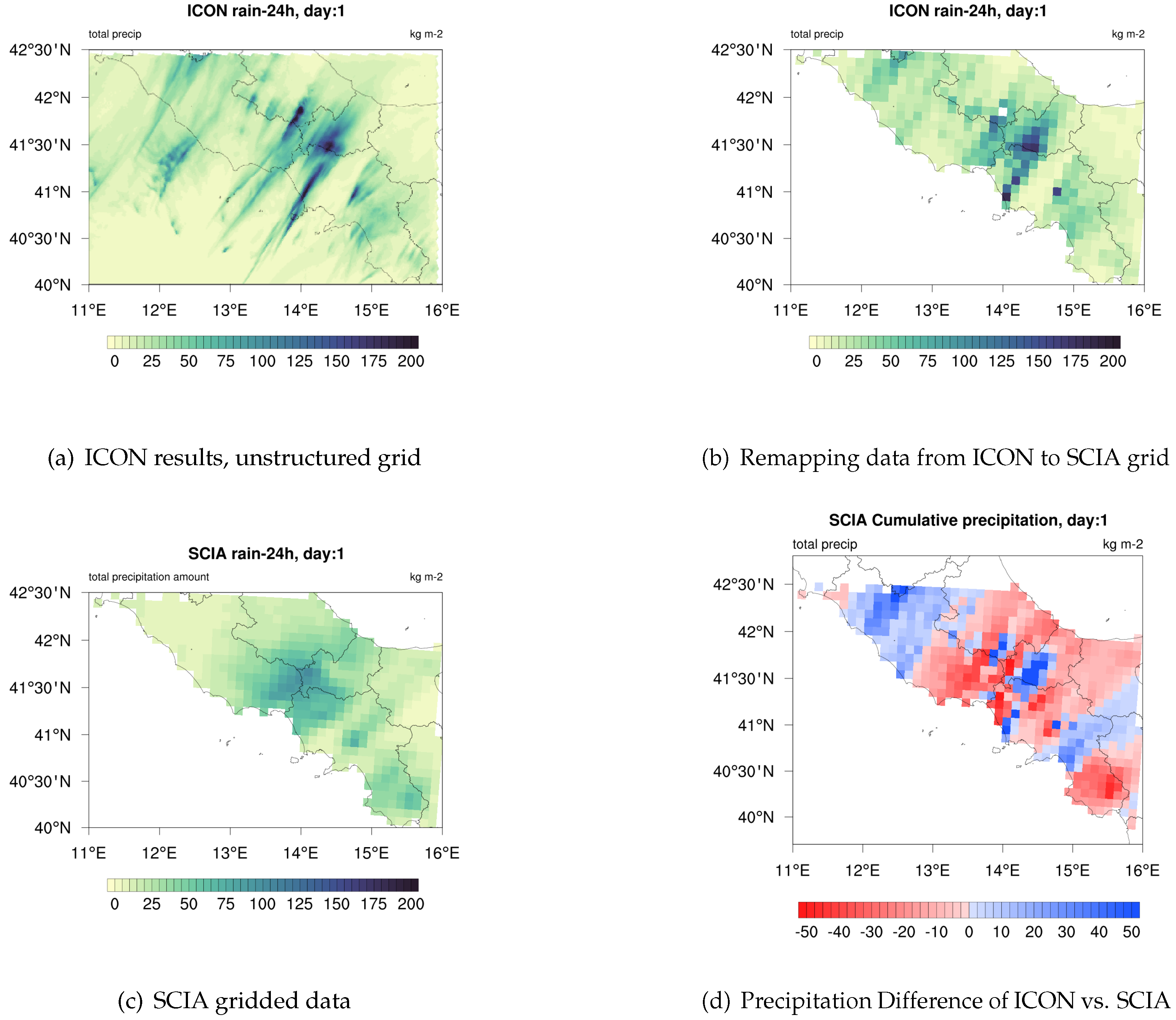
The ICON outputs (at hourly frequency) were processed to calculate statistical values that, as objective metrics, could support the process aiming to find the optimal domain and the optimal configuration in terms of physical parameters. The variables considered for the metric calculation were the daily maximum ( T m a x ) and minimum temperatures ( T m i n ) and the total daily precipitation ( P r ) , using the observational values as terms of comparison. Specifically, the usage of in-situ local stations required the identification of the nearest grid point to the station location. On the other hand, the usage of the grid dataset required appropriate post-processing activity, aiming to remap the daily values from the native ICON grid to the grid of the SCIA dataset. Remapping was performed by means of upscaling from the ICON unstructured grid to the SCIA regular grid, with an Inverse-Distance interpolating technique. Once the ICON output had been remapped on the structured grids, compatible with the observations, model fields could be compared with observed ones. Figure 3 shows the step-by-step transformation process from the native ICON grid to the SCIA grid.
In detail, starting from the ICON results on the unstructured grid at 1.2 km resolution (Figure 3a: rain 24 h), upscaling was done to remap them over an SCIA-like grid (Figure 3b) by means of Inverse Distance interpolation. Successively, the transformed data could be compared to the SCIA data set (Figure 3c) in order to evaluate statistics on which the target function was based, Figure 3d shows the precipitation gap as the difference between data in Figure 3b minus data of Figure 3c). These operations were valid for the grid data, and since local data (read at several weather stations) were also considered in evaluating a devoted target function, the nearest cell centers to the local station coordinates were selected in the ICON results and compared to the station data. More details are given in the following section.

5.2. Objective Target Function

The aim of the work was to find a set of numerical parameters that, by tuning of the empirical physical models of NWP, also significantly influenced the NWP results. Hence, once those parameters were defined, by searching in the space of their feasible configurations (i.e., the hypercube defined by their ranges), the optimized search for the best configuration, was able to minimize the distance between numerical and observed data. To measure that distance, representing an error, a function has to be defined. This function has to take the following factors into account: the day-by-day spatial averaging of the compared data, the time averaging of the same data over the window of observation (i.e., the week of the simulation), the nature of the observed data (Minimum and max temperature, precipitations), and the statistical function to be considered to measure the distance. As explained before, we decided on a single-value objective function.
With these aims in mind, a scalar metric was defined to quantify the distance between the model results and the observational data, in terms of T m i n , T m a x and P r from the SCIA dataset [11]. The minimization of this scalar metric (objective function) guides the process of choice of the optimal domain and the process of optimization of the physical parameters.
The target function adopted here was derived from the statistical terms of the Taylor diagram [5]: the normalized Root Mean Square error (NRMSE), the correlation value ( ρ ) and the standard deviation. Some limitations of this statistical set were evidenced by [6], related to the fact that an overall bias is not considered. For this reason, in the metric introduced here, an additional term was considered, the normalized Mean Absolute Error (MAEN). The standard deviation was neglected, since it is mathematically related to NRMSE and ρ terms. The three terms considered are defined as follows:
ρ = j ( F j F ¯ ) ( O j O ¯ ) j ( F j F ¯ ) 2 j ( O j O ¯ ) 2
M A E N = 1 N c e l l s j = 1 | F j O j | 1 N c e l l s j = 1 O j
N R M S E = 1 N c e l l s j = 1 ( F j O j ) 2 r a n g e ( O j )
In these formulae, F j is the model value for j-th cell, O j is the observed value for the j t h cell or station, since the target function is evaluated against both SCIA-grid and SCIA-stations. In Equation (2) MAEN is normalized by the mean of the observational values, while in Equation (3) the NRMSE by its range, r a n g e ( O j ) (i.e., the distance between maximum and minimum observed values).
The target function considered is defined as:
F o b j = i V w i A j D m a e n i , j + B j D ( 1 ρ i , j ) 0.5 + C j D n r m s e i , j
where V indicates the ensemble of variables vector V = ( T m i n , T m a x , P r ) , D is a scalar index running over the analyzed days (hence D = 7 ). The scalar weight values w i are chosen in such a way that the variables in V are equally weighted. In a similar manner, the scalar quantities A, B and C that weight the single statistical terms are set equal to 0.333.
The objective function in Equation (4) was defined in such a way that optimal performances corresponded to F o b j = 0 , i.e., model values and observations were coincident.

5.3. Automatic Calibration

Several studies have shown that the configuration of an NWP LAM model (developed for a specific area) cannot be directly transferred to other geographical areas [10]. The definition of a suitable model configuration for ICON-LAM over Italy is only at an early stage, so that deep analyses are still required in order to consider the particular orography of the Italian peninsula and its strong interaction with the sea. In the present work, the values of these four parameters were optimized by means of an automatic calibration approach, following a strategy similar to the one presented in [1]. The four parameters (see Table 1) were tuned so as to reduce the distance of the model output from the observational data. The metric adopted to measure the enhancement referred to the baseline settings is described in Equation (4). The optimization of F o b j relies on an Efficient Global Optimization (EGO) approach described in [18], based on the definition of a ‘cheap’ metamodel that replaces the computationally expensive ICON simulations in design space exploration. The aim of the metamodel is twofold. It should be able to set up a relation among F o b j and the selected name list parameters and, then, the Kriging model, [19], guides adaptive sampling of the design space, defined by the chosen name list parameters, in order to find global minima values [18].
Figure 4 illustrates the whole iterative process required to set up the metamodel aimed at finding a promising region in the space of the physical parameters described in Table 1. The process can, ideally, be split into offline and online (or sequential) stages. In the first stage, an a-priori sampling of the Design Space was performed, by means of Latin Hypercube Sampling (LHS) [20]. Within this stage, a test matrix of simulations was designed, in which, for each design vector (containing the values assumed by the design variables), a name list of physical parameters was established, followed by an ICON simulation over the week under investigation. Once the collection of runs necessary to train the metamodel had been defined, they could be executed in parallel on the Turing server. Then, once the results had been post-processed and the metrics obtained, the relationship between the physical parameters and F o b j could be stated in the metamodel definition.
The iterative stage is related to adaptive sampling. The successive ICON simulations are identified by using a promising design variables vector relying on the Expected Improvement (EI) auxiliary function [18], based on the current F o b j minimum value and metamodel predictions and uncertainties, which predict the enhancement of F o b j value if a new ICON evaluation is performed with the suggested configuration. Hence, the suggested sample (from which a new name list is derived) is evaluated with ICON, and the resulting F o b j is added to the metamodel database. Then, a metamodel update follows, with a new sample and new ICON evaluations. This iterative process can be stopped by a criterion, based on, for example, a computational budget, to limit the number of ICON-allowed simulations, or, alternatively, it can rely on a threshold value for F o b j or EI.
In this work, two different metamodels were set: the first defined an F o b j for SCIA-gridded data, F g r i d d e d o b j , and the second for SCIA-stations, F s t a t i o n s o b j . These metamodels worked in parallel, since they were fitted on the same database of ICON simulations, but post-processed separately to obtain F s t a t i o n s o b j and F g r i d d e d o b j . In the iterative stages, both of them suggested their own design vectors by means of the maximum EI, and, hence, two ICON sets of simulations were started.
The computational budget for the off-line stage involved a test matrix of thirty-six ICON simulations, plus the baseline set of ICON runs with the configuration of physical variables inherited from [10]. In the adaptive stage, the two metamodels drove the optimization, each suggesting its own candidate name list that ICON simulated, and, then, updated the metamodel once the results were post-processed. In this stage, further ICON evaluations were performed, to reach a total of 130 runs.

6. Results

In this section, the results from the domain sensitivity and the automatic calibration performed with a surrogate-based optimization are described. The former step is discussed in the following subsection. Once the optimal domain was defined, the automatic calibration process was applied and the results are presented in Section 6.2.

6.1. Domain Selection: Results

Since ICON-LAM was tested for the first time on the region under study and with a high resolution (i.e., ∼1 km), domain sensitivity, to assess the influence of the boundary location on the solution accuracy, was performed. As already explained, three domains of different sizes were evaluated (DOM1 was the smallest sized domain, DOM2 in the middle and DOM3 the largest). In the evaluation process, we also considered, as reference, the results of a COSMO simulation described in [13], where the configuration of the model was similar to the present ICON-LAM setting in terms of grid resolution, while the domain was comparable to DOM1 (Figure 1 and Table 2).
The results obtained over the three domains were compared over the central area, common to the three domains. Of course, SCIA grid data and local stations were extracted for this target area. As explained in the previous section, the objective function (Equation (4)) was used to measure the effectiveness of the three domains. It is worth noting that the final choice of the optimal domain was also driven by the CPU request, which increased considerably with domain size, as shown successively. In order to check the reliability of F o b j for the proper selection of the optimal domain, the Taylor diagrams [5] were also used as a supporting tool to compare the results. The Taylor diagrams are graphical methods useful to compare model output with reference data, based on the metrics involved in the evaluation of F o b j . However, despite its reliability, this graphical method does not lend itself to use in an automatic calibration algorithm.
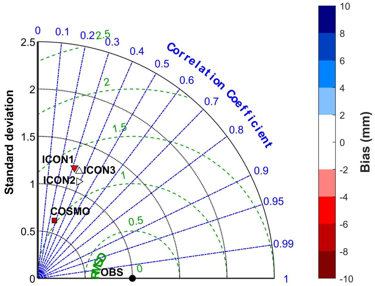
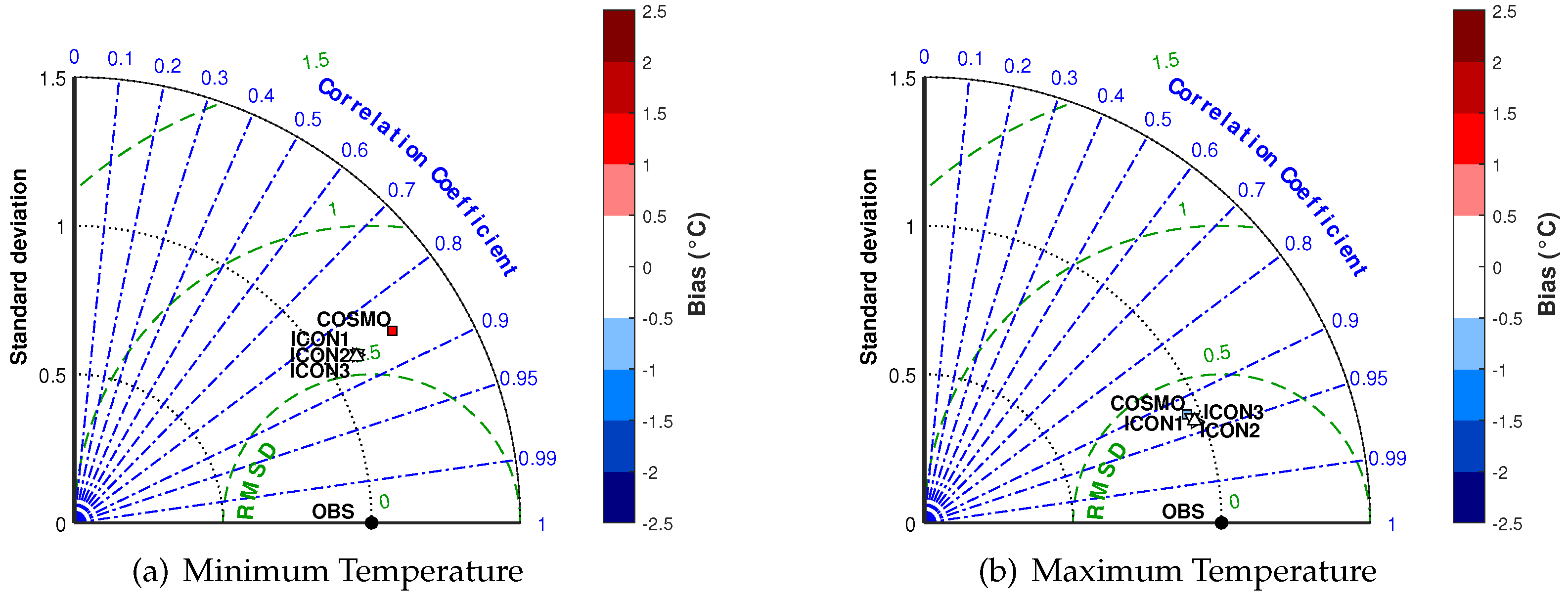
The Taylor diagrams resulting from comparison with the SCIA grid dataset are shown in Figure 5 and Figure 6, averaged over the week considered. An evident result was represented by the better performance of ICON against COSMO, especially for T m i n and P r . However, an analysis of the diagrams did not allow the selection of the best domain, even if DOM2 seemed to perform better for P r .
In fact, while the P r difference among ICON domains could be appreciated, this was hard to do graphically, since the solutions were very close to each other, as can be observed in Figure 6.
Figure 7 shows the results of the evaluation in terms of F o b j values. Specifically, in Figure 7b it is possible to compare the global metric obtained with the three ICON domains and with COSMO. The results show that the DOM2 and DOM3 performed in a similar manner and both out-performed DOM1 and COSMO. In order to check the roles played by the three variables analyzed in achieving the results, their contributions to the global value of F o b j are shown in Figure 7a. In terms of T m a x and P r , the model performed better with DOM2, while for T m i n , better results were obtained with DOM3.
Taking into account the computational loads required by the simulations over the three domains, DOM2 was selected as the optimal one, since its performances were comparable with DOM3, but it was less expensive in terms of CPU. DOM2 was used in the second phase of this work for the calibration of the physical parameters.

6.2. Automatic Calibration: Results

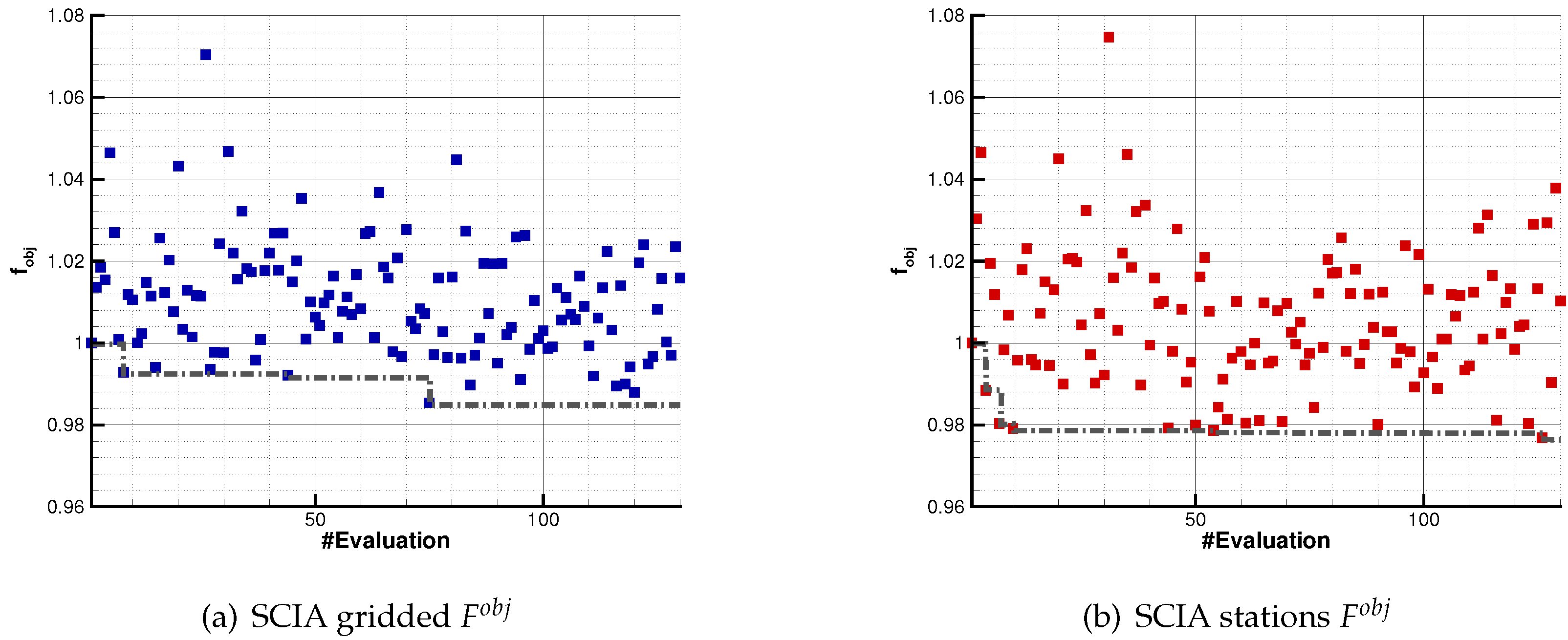
According to the methodology described in Section 5.3, a series of simulations were performed with ICON-LAM, aimed at minimizing the target function. Figure 8 shows the evolution of F g r i d d e d o b j and F s t a t i o n s o b j resulting from the ICON run, and, along with the single F o b j realizations, the lower envelope was overlaid with the dashed gray lines, representing the evolutionary history of the minimum values F o b j . It can be seen that the trend of these functions narrowed in the region of lower values, as the number of iterations increased, meaning that the algorithm was exploring regions of the design space where ICON, on average, performed better than the reference name list. The two functions (grid and stations) were only poorly correlated. This circumstance could be ascribed to the following factors: the interpolation process grid data underwent during generation; the interpolation process necessary to upscale ICON results over a coarser grid; the short observation period could have influenced the poor correlation, independently of the other factors. These aspects will be investigated in future work.
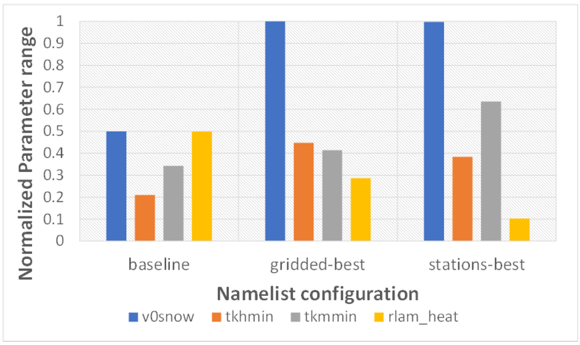
Table 3 reports the values of the design parameters, for the baseline and for the best configurations obtained considering, respectively, SCIA-grid and SCIA-stations. The corresponding values of F o b j are provided too. The histogram plot of Figure 9 shows the normalized values (with respect to their variability ranges) of the four parameters, highlighting the extent of their variations in the optimal configurations with respect to their original values. These results revealed that the algorithm moved in the design space towards a common direction, in both grid and station optimization processes. Compared to the baseline parameters, it can be noted that the v0snow value moved towards its upper bound in both cases, tkhmin increased its values by around 40% of its range; tkmmin increased more in the Station case; rlam-heat decreased, more consistently so for the Station case.
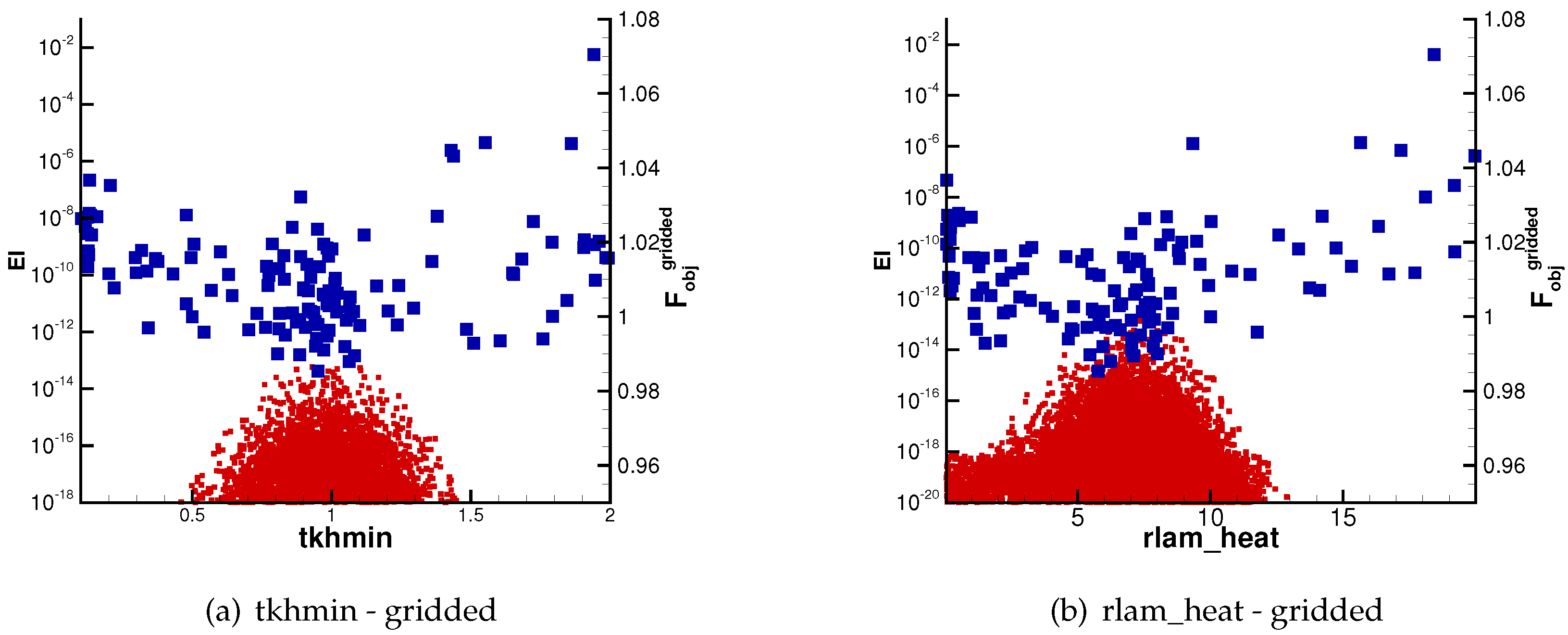
Other useful information for future steps in the optimization campaign were also derived from the regions of design space of the variables in Table 3, characterized by higher expected improvement.
For example, for the SCIA-gridded data, (Figure 10a) the best values for tkhmin slightly shifted from the baseline values and a promising region was found by sampling the EI function (described in Section 5.3) in the range of 0.8 ÷ 1.1 . This information could be useful as a new reduced range of exploration for tkhmin, to be reconsidered in order to verify its interaction with other variables in future activities with additional physical parameters involved.
The best values for the parameter rlam_heat, against SCIA-gridded data (Figure 10b), were lower compared to the baseline ones and the promising range was 5 ÷ 9 c.a. On the other hand, the parameters v0snow and tkmmin revealed quite noisy behavior, with v0snow (not shown here), characterized by a triple region of improvement, clustered on the upper and lower bounds, and also on medium values (around 20).
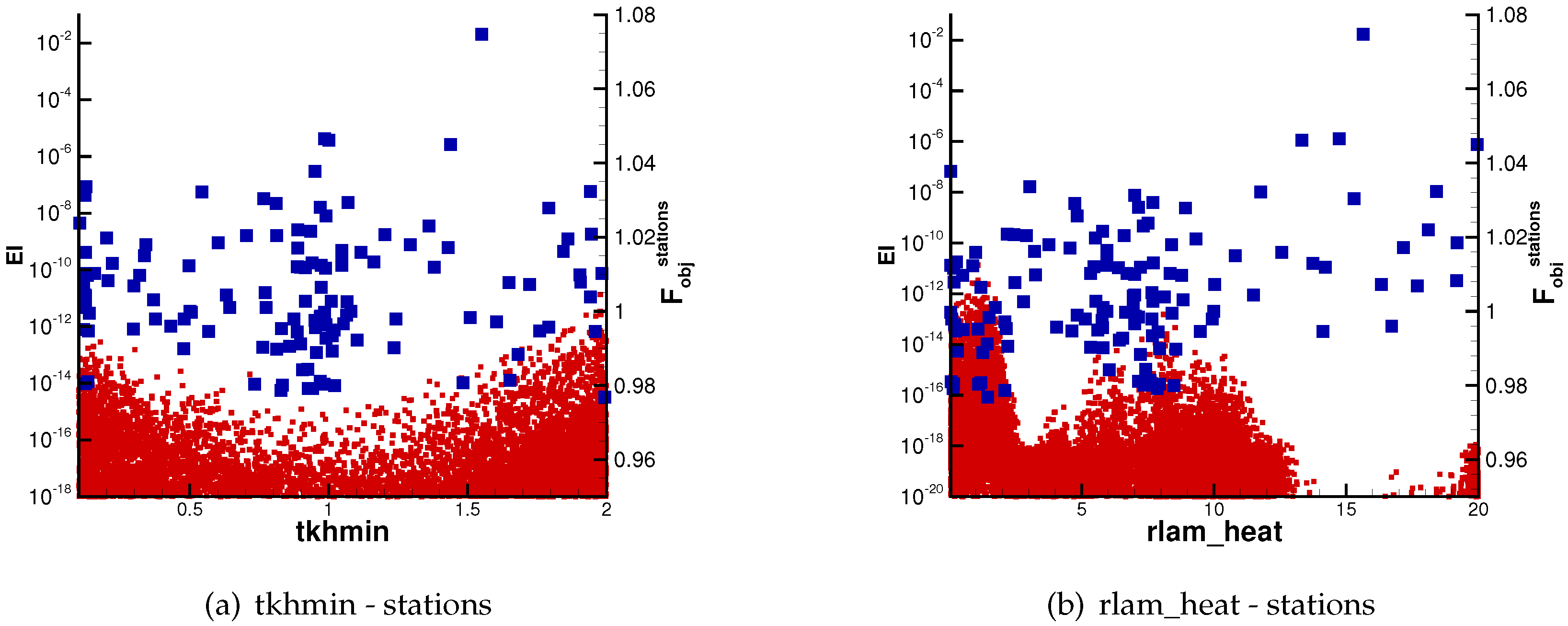
Against SCIA-station data (Figure 11a,b), for tkhmin, the expected improvement was higher in upper and lower boundaries, while for rlam_heat it was also high in the range close to the lower boundary, in addition to the range of values already highlighted in Figure 10b. It can be seen that, for some variables, e.g., rlam_heat, there was an overlapping region of expected improvement, which suggests the possibility that, with further sequential runs, the solutions could converge.

6.2.1. Analysis of Results against Grid Dataset

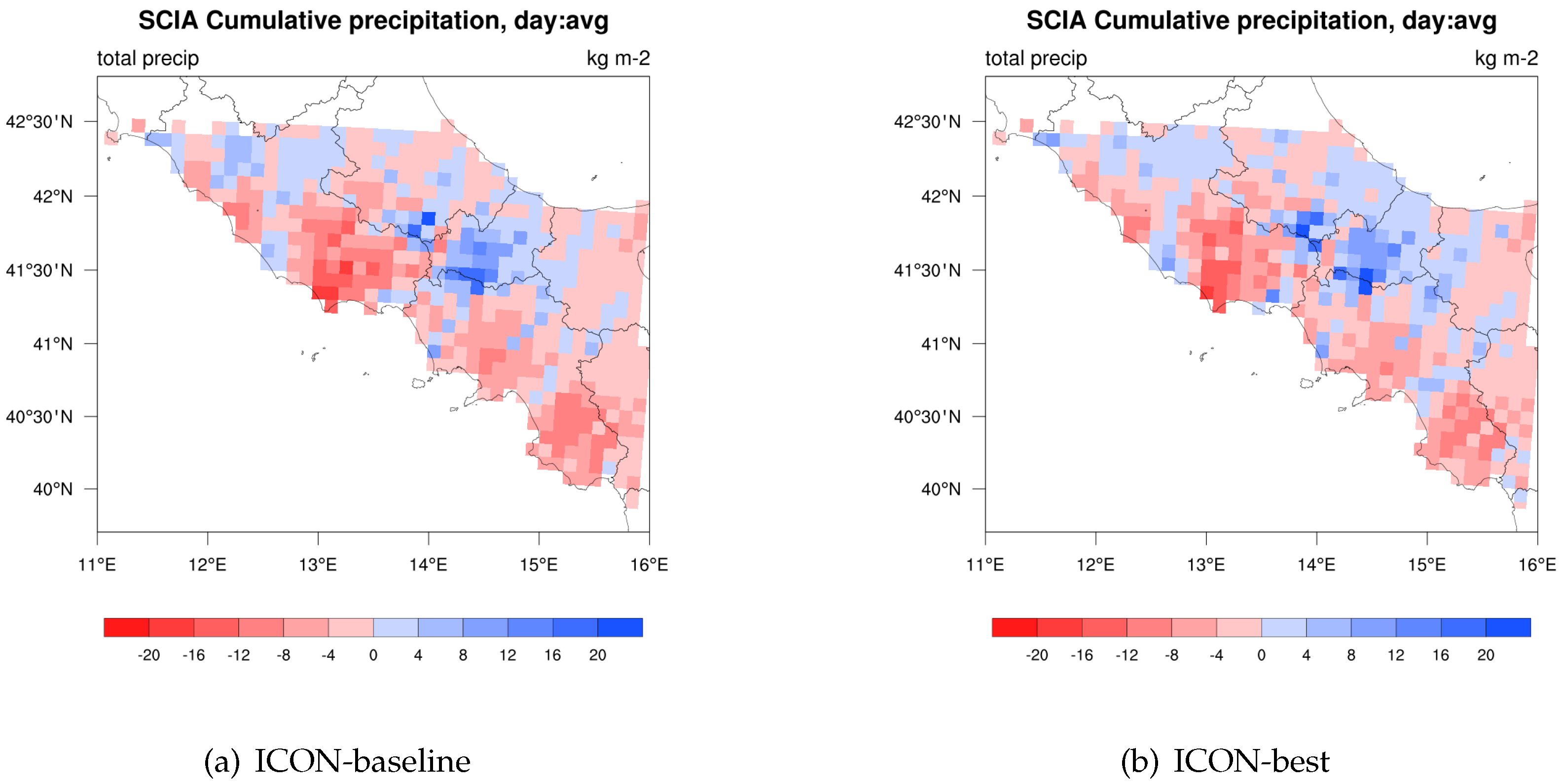
Figure 12 shows the comparison between the model biases obtained using the baseline and the optimal configuration, considering the SCIA-Grid dataset as reference. The maps represent the difference between the daily precipitation simulated by the model and that observed, averaged over the seven days considered. Even though the differences were not so evident, it is important to keep in mind that the enhancement of the metric F o b j was about 1.5% with respect to baseline, and that the contribution could be ascribed to a cumulative precipitation improvement of about 3% (while for the other two variables the improvement was 1% for minimum temperature and 0.5% for maximum temperature).
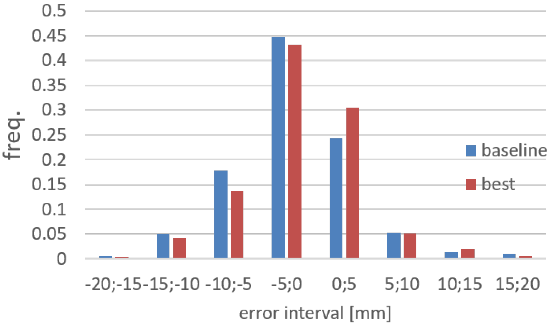
In order to quantify the distribution of the cumulative precipitation error plotted in the maps of Figure 12, a frequency histogram was elaborated (Figure 13), from which it is evident that both the model configurations tended to underestimate the precipitation, but the best one caused a shift toward central values (characterized by lower errors).
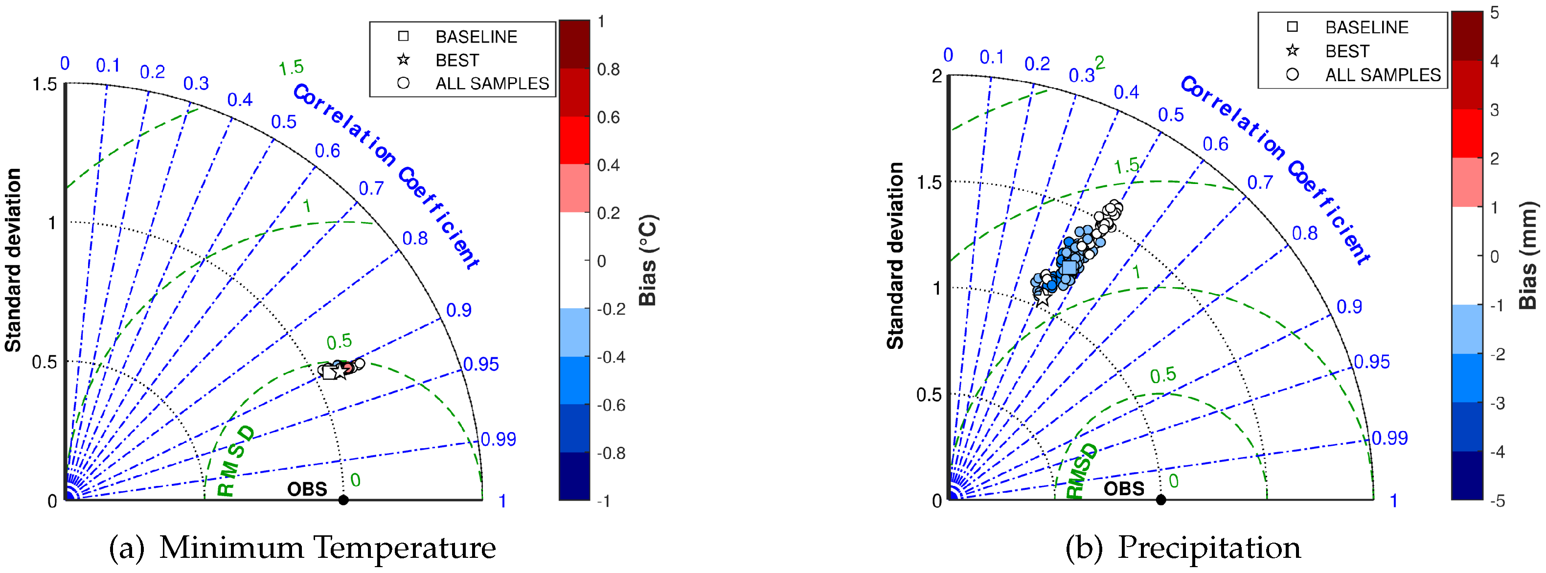
The graphical method, based on Taylor diagrams, could be useful to check if the calibration process, driven by the minimization of F o b j , is working in the right direction. Figure 14 shows the Taylor’s diagram including results from all the samples of the automatic calibration performed over DOM2. The data employed to define the diagrams were averaged in space and time, as already done in the definition of F o b j (Equation (4)). T m i n (Figure 14a) shows little sensitivity in terms of NRMSE, bias and standard deviation. In this case, the best sample enhanced performances in terms of bias and correlation with respect to the baseline values. The diagram related to P r (Figure 14b) shows a larger spread in terms of standard deviation and NRMSE. The best configuration facilitated enhancements in terms of bias, standard deviation and NRMSE, while the correlation slightly reduced. On the contrary, T m a x (Taylor’s diagram not shown here) was not very sensitive to the tuning of the physical parameters involved in this optimization.

6.2.2. Analysis of Results against Station Data

According to the values of Table 3, the optimized name list facilitated an improvement of 2.3% with respect to the baseline configuration when in-situ station data were considered as the reference. As defined in Equation (4), the results were obtained as an average among the three variables, over all the stations and over the whole week considered. Hence, if we look at specific stations, there is the possibility to find the worst, equal or better results. Figure 15 shows an example of the comparison between model results and observed data for two in-situ stations, in terms of daily minimum and maximum temperatures and cumulative precipitation, considering both the baseline name list configuration (blue curve) and the optimized configuration (red curve). It is evident that P r for Itri station and T m i n for Fondi station experienced clear enhancements with the new configuration.
Figure 16 shows the scatter plots of the station observed vs, simulated values (highlighting the correlation between them) for the reference name list, an intermediate name list and the optimal name list configurations, in such a way that the evolution of the distance between observed and forecast data, through the search in the design variable space, can be appreciated by noticing enhancement of the statistics in the latter plots compared to the references. In each scatter plot, the value of the R 2 index is also indicated, as a dashed line, as is the ideal curve indicating the equivalence between model (y axis) and observed data (x axis). The first row of scatter data (Figure 8a–c) is relative to the reference name list configuration. The central row (Figure 8d–f) refers to an intermediate name list configuration (iteration no. 54, see also Figure 8b), characterized by optimum performances for P r , and T m i n , while T m a x was slightly worse than the baseline, as can be noted by comparing the respective R 2 values. The last row refers to the ’best’ configuration (iteration no. 126 in Figure 8b), which out-performed the baseline name list in each of the target variables, even if the precipitation scatter plot is characterized by a lower R 2 index when compared to Figure 16d. It should be kept in mind that the correlation index is only one among the three metrics considered in F o b j .

6.3. Model Validation

As already stated, the week 1–7 July 2019, was chosen for an independent evaluation test, because it was characterized by a dry weather regime, e.g., the 2-m maximum temperature, averaged over the region and over the week, reached 32 °C, while the average minimum temperature reached 19 °C, with rare and isolated rainfall.
The two optimal configurations previously defined (‘grid-best’ and ‘station-best’) were tested against the reference one (‘baseline’). Figure 17 shows the histogram plot of the comparison among the three configurations in terms of objective function values. In particular, in Figure 17a, the three name lists are compared assuming the grid data as reference. In this case, it is evident that the ’grid-best’ performed slightly better than the ‘baseline’, while ‘station-best’ was not able to improve performances. In Figure 17b the three name lists are compared against station data. In this case, both ‘grid-best’ and ‘station-best’ provided better results than the baseline.
In detail, we found that the two ‘’best’ configurations showed optimal performances on the forecast of the 2 m minimum temperature, out-performing, in both cases (grid and local data), the baseline performances. Good behavior in precipitation forecast for the name lists was recorded against station data. Some difficulties were encountered in simulating the daily maximum temperature, especially for the‘’station-best’ configuration. This behavior could probably be ascribed to the fact that these configurations were trained in a winter period.
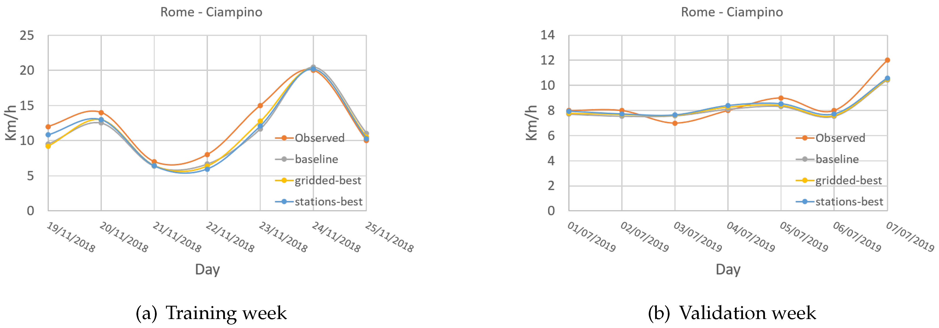
Moreover, an independent verification of the tuning results for other forecast variables, not processed by the optimization algorithm, was performed in 2 m relative humidity, mean wind speed and gusts at 10 m against selected station data (grid data for these variables are not currently available). In detail, data from seven weather stations were selected for the evaluation, for both the training week (in winter) and the validation one (in summer). The selected stations were located at four airport stations (Napoli Capodichino, Grazzanise, Pratica di Mare and Rome Ciampino) and three other locations (Capri, Trevico and Pontecagnano). Figure 18 shows the mean daily values of wind speed at Rome Ciampino (observational and model values obtained with the three configurations considered), from, respectively, 19–25 November 2018 (a), and 1–7 July 2019 (b). ICON reproduced the wind behavior well, and, in particular, it is worth noting that both the ‘best’ configurations out-performed the baseline one. Similar behaviors were recorded for the other stations (not shown).
A similar analysis was performed in terms of relative humidity at 2 m. Figure 19 shows the mean daily values at Napoli-Capodichino (model and observations), respectively, in the winter week (a), and the summer week (b).
Finally, a synthesis of the forecasting skills of the optimized name lists, in both winter and summer weeks, is presented in Figure 20 for the three variables (Relative humidity, mean wind speed and gusts), in terms of objective function values defined in Equation (4) normalized against the values assumed with the baseline name list.
In the validation week, the relative humidity (Figure 20a) showed that the optimized name lists were not able to improve performances (values of the objective functions were greater than 1.0), while in the winter week the grid-best name list out-performed the baseline. The average wind speed (Figure 20b) was well predicted in the validation week by both the ’best’ name lists. In particular, the station-best showed optimal performances in both weeks. Finally, Figure 20c shows that the optimized configurations were not able to improve the gust forecasts in the winter week, while different behavior was found in the validation period, where the station-best out-performed the reference name list.

7. Discussion

This work represents a first approach to set up a preparatory methodology for an optimization campaign for a large set of physical parameters, aimed at defining an optimal ICON-LAM model configuration at high resolution over southern Italy, for operational runs. In fact, the input parameters considered for optimization in this work were only a few of the huge amount of parameters potentially involved.
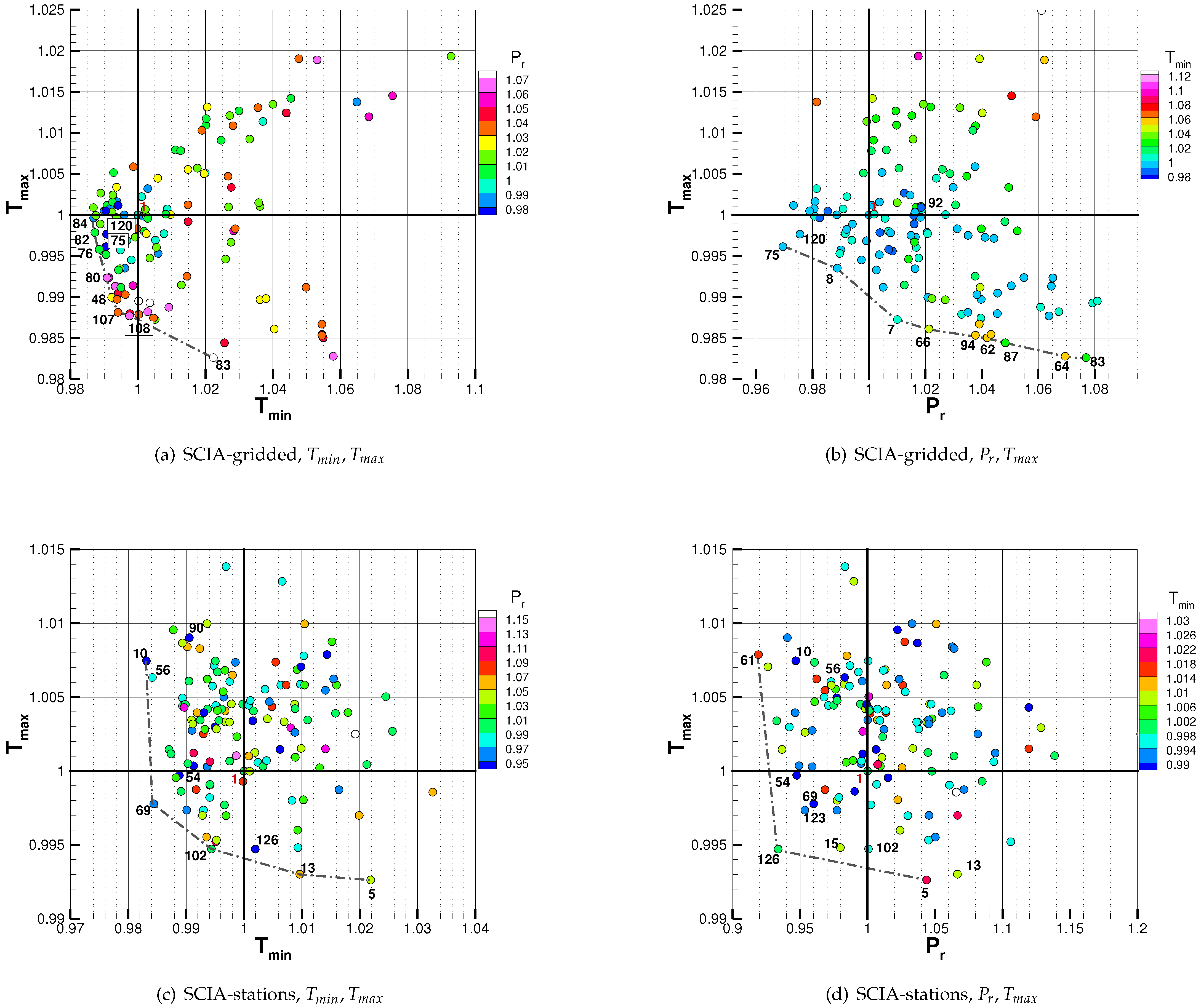
The three terms that compose the weighted, single objective F o b j , representing the three observed variables to be optimized, behave differently, and, hence, the final F o b j best solution often does not coincide with the "partial" best solutions for the single variables ( T m i n , T m a x and P r ). This is due to the fact that optimal parameters for a given variable may conflict with those for other variables, and, furthermore, this consideration also holds for the three different metrics involved in Equation (4), as also stated in Duan et al. [1], who also showed how the optimization of a single meteorological variable in a single objective functional optimization can out-perform, for the specific variable, an optimization involving an objective function that averages two or more variables, even if the latter results in a non-dominated configuration, i.e., is better than the reference configuration, but worse than the individual one. This issue is due to the conflicting natures of the objectives. In this work, the issue of multi-objective optimization was treated as a single value problem. For this reason, in order to verify that the optimal solutions found improved all the variables involved in V, compared to the reference solution, a Pareto frontier was plotted, for both the optimization problems considered, i.e., against grid and station data. Since V has three components, a 3D plot should be visualized, but this confuses the 2D support. For this reason, Figure 21 displays 2D plots (i.e., T m a x vs. P r and T m a x vs. T m i n ) to overcome this visualization issue. To support an effective classification of the best sample, the third variable neglected is displayed by means of a colour scale applied to the markers representing the sample points. These kinds of plot are characterized by four regions (quarters), generated by the straight lines passing through the point with coordinates ( 1 , 1 ) that represents the baseline objective function (or reference point). The region I (third quarter, where both the F o b j coordinates are less than 1) is the region characterized by samples that have out-performed the baseline configuration, also known as the non-dominated region, Region II includes samples that enhance only the F o b j of the vertical axis (i.e., y < 1 and x > 1 ). Region III has x < 1 and y > 1 and only the F o b j on the horizontal axis is enhanced. Finally, samples in region IV ( x , y > 1 ) are dominated by the reference point. Figure 21a,b show the regions for the optimization process conducted against grid data. In detail, Figure 21a shows the samples (ICON runs) in the plane ( T m i n , T m a x ) . A grey dashed line links the samples from the outer solutions, namely the best one in terms of T m a x (labeled with iteration number 83) up to the best values found for T m i n (iteration 84). A Pareto Frontier can be approximated in this plane, going from the latter point (iteration 84) to the one labeled 108, linking the solutions of region I, which represent the non-dominated samples. As stated before, the colour scale of the samples represent the F o b j values of the variable not represented in the plane (in this case it is P r ). The samples that belong to the Pareto frontier are characterized by colours going from light green to red, meaning that F o b j P r > 1 , while the samples labeled with 75 and 120, belonging to the region of non-dominated solutions, are quite near the calculated Pareto frontiers, representing, respectively, the best sample and the second best in terms of F o b j P r . In fact, in Figure 21b, which displays the plane ( P r , T m a x ) , sample 75 belongs to the Pareto frontiers, and sample 120 is quite near this boundary, meaning that these solutions are also optimal in terms of precipitation. From this analysis, it can be assumed that the optimization process with respect to grid data identified solutions that enhanced performances for all the involved variables.
Figure 21c,d refer to the optimization process against station-data. Figure 21c shows the calculated Pareto frontier and highlights the best solutions for T m a x and T m i n , i.e., 5 and 10, respectively, while the non-dominated ones are 69 and 102. The colour of sample markers here help to identify the performances in terms of P r . In the non-dominated region, sample 54 was noteworthy, while sample 126, even though it fell in region II, was the best solution identified in the optimization process against the station data. In fact, in the plane ( P r , T m a x ) (Figure 21d), it was undoubtedly the best element. Sample 54 fell in the non-dominated region, also in this plane. We verified that an approach that promotes the non-dominated samples, as proposed in [8], would reward this solution (i.e., 54) too, and, therefore, it could be considered a valid methodology to adopt in future works.
The differences recorded in terms of optimal parameters, when considering grid and local data, were already described in Section 6.2 and shown in Table 2. The differences can be ascribed to several factors, such as the short time window of the training dataset. However, an aspect worth investigating is related to the interpolation technique adopted to fulfil conservative up-scaling of the ICON output to the grid of observational data. This issue could be an influencing feature when dealing with grid upscaling that involves grids with very different sizes, such as the case of a very high-resolution model grid, projected over a grid of observed data, where the ratio between source and target cell is larger than 5.

8. Conclusions

In this paper, an automatic calibration methodology was implemented to optimize the parameters of the high resolution ICON-LAM over a region located in southern Italy. As a first step, an assessment of the effects of the size domain on the solution was performed, in order to select an optimal domain, able to minimize the distance between modeled and measured meteorological variables, e.g., minimum and maximum temperature and daily precipitation. Then, in the automatic calibration procedure, only a limited number of physical parameters was considered for tuning, starting from a reference ICON configuration inherited from a previous work. The multi-objective nature of the calibration was, here, transformed into a single-objective surrogate-based optimization, since the scalar objective function was a linear combination of the distance between model data and observations, averaged over the selected time window. Two distinct metamodels drove the adaptive sampling, measuring, respectively, distance from grid observed data, and local stations. This analysis made it possible to evaluate the effects of the nature of the data on the optimization results. The grid data metamodel resulted in a smoother landscape than the in-situ data. Moreover, the optimal values of the tuned physical parameters showed that the optimization process moved in a common direction. Starting from the reference parameters, tkhmin increased and, according to [13,21,22], this implies that the turbulent kinetic energy is maintained in stable condition, eliminating strong inversion. Moreover, its increase caused a growth in precipitation, since it increased small convective cloudiness. The rlam_heat decreased and its reduction caused increasing instability, thus, influencing precipitation. However, the relevance of this parameter was largest under calm anticyclonic conditions with a stable nocturnal boundary layer. In the experiments presented, v0snow did not show a clear influence on the objective function. The best elements were both characterized by almost upper boundary values, but there was also a trend that recognized the area of improvement towards the lower limits or towards the central area. It was evident that there were discrepancies between results against grid and local station data, but this mismatch could be ascribed, among other causes, to the interpolation technique that was used to project the ICON output on the grid of observational data. A check in the space of the objective function performed at the end of the optimization process indicated that the algorithm moved towards a set of solutions that were non-dominated by the reference one (the improvement of metrics on the local stations side was 2.3%, while the improvement on the grid data side was 1.5%), and, hence, approximated a Pareto frontier. Finally, it is worth mentioning that the period chosen for the optimization (19–25 November 2018) was characterized by huge precipitation and strong winds, and of course the optimization process was mainly aimed at having a better fit of the cumulative daily precipitation. For this reason, the best name lists resulting from the optimization stage were tested for a validation week in a different season, showing that the reference configuration could be out-performed anyway. Furthermore, performances of the forecast of additional variables were also tested, showing an improvement in some of them, i.e., the mean wind speed. The promising results of the presented approach represent the basis for the next steps in this research field, involving a longer training period, and more variables and parameters to be tuned, in order to establish the best configuration for the region under investigation.

Author Contributions

Conceptualization, D.C. and E.B.; methodology, D.C.; software, D.C., A.L.Z. and M.M.; validation, D.C., A.L.Z. and M.M.; formal analysis, D.C.; investigation, D.C.; writing—original draft preparation, D.C. and E.B.; writing—review and editing, M.M., A.L.Z. and E.B.; visualization, D.C. and A.L.Z. All authors have read and agreed to the published version of the manuscript.

Funding

This research received no external funding.

Institutional Review Board Statement

Not applicable.

Informed Consent Statement

Not applicable.

Data Availability Statement

Data are stored at CIRA supercomputing center and are available on request.

Acknowledgments

The authors wish to thank: A. Mastellone and C. De Lucia (CIRA) for the support provided in the installation of ICON code; D. Reinert and D. Rieger (DWD) for their useful advices on ICON model.

Conflicts of Interest

The authors declare no conflict of interest.

References

  1. Duan, Q.; Di, Z.; Quan, J.; Wang, C.; Gong, W.; Gan, Y.; Ye, A.; Miao, C.; Miao, S.; Liang, X.; et al. Automatic Model Calibration: A New Way to Improve Numerical Weather Forecasting. Bull. Am. Meteorol. Soc. 2017, 98, 959–970. [Google Scholar] [CrossRef]
  2. Neelin, J.D.; Bracco, A.; Luo, H.; McWilliams, J.C.; Meyerson, J.E. Considerations for parameter optimization and sensitivity in climate models. Proc. Natl. Acad. Sci. USA 2010, 107, 21349–21354. [Google Scholar] [CrossRef] [PubMed]
  3. Bellprat, O.; Kotlarski, S.; Lüthi, D.; De Elía, R.; Frigon, A.; Laprise, R.; Schär, C. Objective calibration of regional climate models: Application over Europe and North America. J. Clim. 2016, 29, 819–838. [Google Scholar] [CrossRef]
  4. Voudouri, A.; Avgoustoglou, E.; Carmona, I.; Levi, Y.; Bucchignani, E.; Kaufmann, P.; Bettems, J.M. Objective Calibration of Numerical Weather Prediction Model: Application on Fine Resolution COSMO Model over Switzerland. Atmosphere 2021, 12, 1358. [Google Scholar] [CrossRef]
  5. Taylor, K.E. Summarizing multiple aspects of model performance in a single diagram. J. Geophys. Res. Atmos. 2001, 106, 7183–7192. [Google Scholar] [CrossRef]
  6. Gleckler, P.J.; Taylor, K.E.; Doutriaux, C. Performance metrics for climate models. J. Geophys. Res. Atmos. 2008, 113, D06104. [Google Scholar] [CrossRef]
  7. Chiandussi, G.; Codegone, M.; Ferrero, S.; Varesio, F. Comparison of multi-objective optimization methodologies for engineering applications. Comput. Math. Appl. 2012, 63, 912–942. [Google Scholar] [CrossRef]
  8. Gong, W.; Duan, Q.; Li, J.; Wang, C.; Di, Z.; Ye, A.; Miao, C.; Dai, Y. Multiobjective adaptive surrogate modeling-based optimization for parameter estimation of large, complex geophysical models. Water Resour. Res. 2016, 52, 1984–2008. [Google Scholar] [CrossRef]
  9. Zängl, G.; Reinert, D.; Rípodas, P.; Baldauf, M. The ICON (ICOsahedral Non-hydrostatic) modelling framework of DWD and MPI-M: Description of the non-hydrostatic dynamical core. Q. J. R. Meteorol. Soc. 2015, 141, 563–579. [Google Scholar] [CrossRef]
  10. De Lucia, C.; Bucchignani, E.; Mastellone, A.; Adinolfi, M.; Montesarchio, M.; Cinquegrana, D.; Mercogliano, P.; Schiano, P. A Sensitivity Study on High Resolution NWP ICON-LAM Model over Italy. Atmosphere 2022, 13, 540. [Google Scholar] [CrossRef]
  11. Desiato, F.; Lena, F.; Toreti, A. SCIA: A system for a better knowledge of the Italian climate. Boll. Geofis. Teor. Appl. 2007, 48, 351–358. [Google Scholar]
  12. Avgoustoglou, E.; Voudouri, A.; Khain, P.; Grazzini, F.; Bettems, J.M. Design and Evaluation of Sensitivity Tests of COSMO Model Over the Mediterranean Area. In Perspectives on Atmospheric Sciences; Karacostas, T., Bais, A., Nastos, P.T., Eds.; Springer International Publishing: Cham, Switzerland, 2017; pp. 49–54. [Google Scholar]
  13. Bucchignani, E.; Voudouri, A.; Mercogliano, P. A Sensitivity Analysis with COSMO-LM at 1 km Resolution over South Italy. Atmosphere 2020, 11, 430. [Google Scholar] [CrossRef]
  14. Seth, A.; Giorgi, F. The effects of domain choice on summer precipitation simulation and sensitivity in a regional climate model. J. Clim. 1998, 11, 2698–2712. [Google Scholar] [CrossRef]
  15. Goswami, P.; Shivappa, H.; Goud, S. Comparative analysis of the role of domain size, horizontal resolution and initial conditions in the simulation of tropical heavy rainfall events. Meteorol. Appl. 2012, 19, 170–178. [Google Scholar] [CrossRef]
  16. Leduc, M.; Laprise, R. Regional climate model sensitivity to domain size. Clim. Dyn. 2009, 32, 833–854. [Google Scholar] [CrossRef]
  17. Song, I.S.; Byun, U.Y.; Hong, J.; Park, S.H. Domain-size and top-height dependence in regional predictions for the Northeast Asia in spring. Atmos. Sci. Lett. 2018, 19, e799. [Google Scholar] [CrossRef]
  18. Jones, D.; Schonlau, M.; Welch, W. Efficient Global Optimization of Expensive Black-Box Functions. J. Glob. Optim. 1998, 13, 455–492. [Google Scholar] [CrossRef]
  19. Sacks, J.; Welch, W.; Mitchell, T.; Wynn, H. Design and Analysis of a Computer Experiments. Stat. Sci. 1989, 4, 409–435. [Google Scholar] [CrossRef]
  20. McKay, M.; BeckMan, R.; Conover, W. A comparison of three methods for selecting values of input variables in the analisys of output from a computer code. Technometrics 1979, 21–22, 239–245. [Google Scholar]
  21. Voudouri, A.; Khain, P.; Carmona, I.; Avgoustoglou, E.; Bettems, J.; Grazzini, F.; Bellprat, O.; Kaufmann, P.; Bucchignani, E. Calibration of COSMO Model, Priority Project CALMO, Final Report. COSMO Technical Report. 2017. Available online: http://www.cosmo-model.org/content/model/cosmo/techReports/docs/techReport32.pdf (accessed on 16 May 2022).
  22. Voudouri, A.; Khain, P.; Carmona, I.; Bellprat, O.; Grazzini, F.; Avgoustoglou, E.; Bettems, J.; Kaufmann, P. Objective calibration of numerical weather prediction models. Atmos. Res. 2017, 190, 128–140. [Google Scholar] [CrossRef]
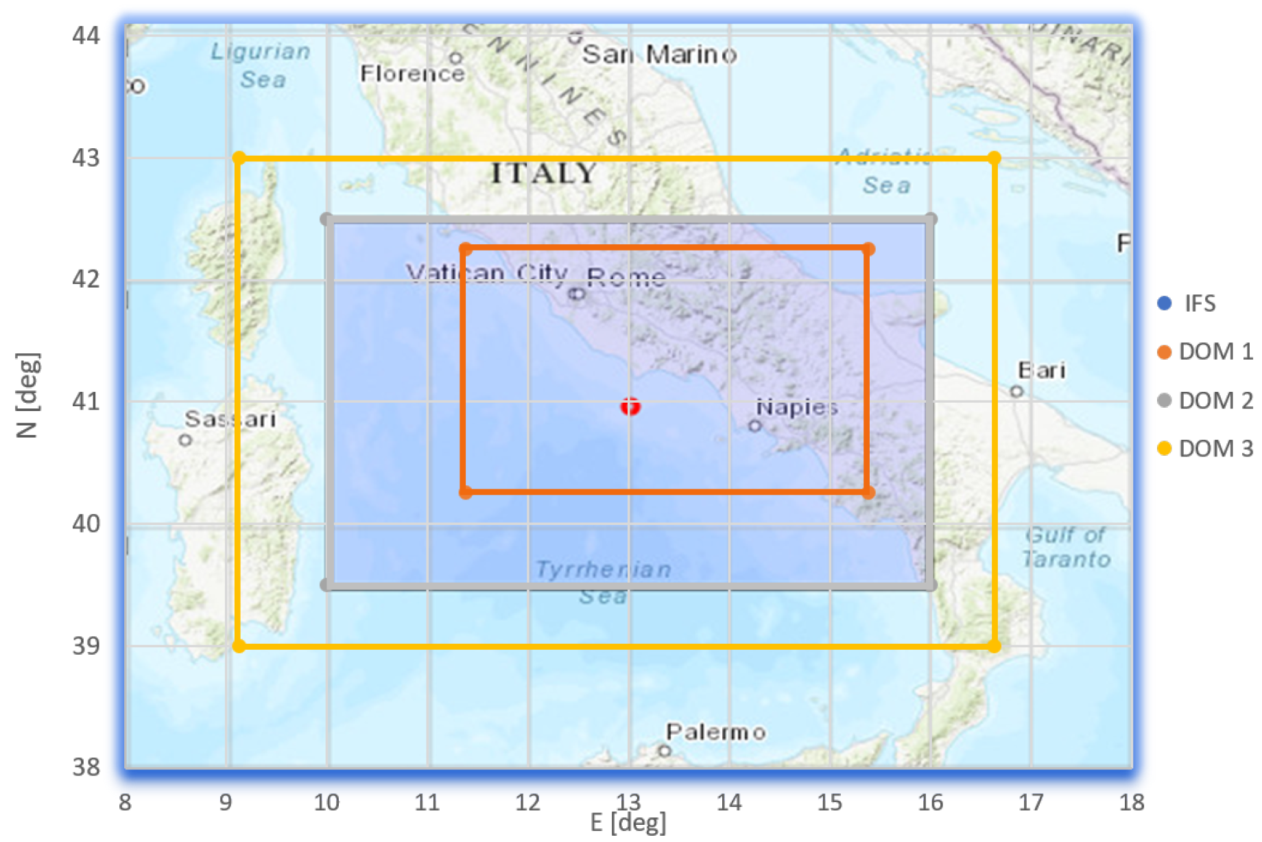
Figure 1. The computational domains DOM1, DOM2 and DOM3.
Atmosphere 14 00788 g001
Figure 2. Distribution of SCIA stations, for (a) Min T and Max T, (b) Precipitation.
Atmosphere 14 00788 g002
Figure 3. Example of post-processing steps necessary to compare ICON results with SCIA grid dataset for daily precipitation.
Atmosphere 14 00788 g003
Figure 4. Metamodel-based optimization set up: Flowchart.
Atmosphere 14 00788 g004
Figure 5. Taylor’s Diagram for the comparison of the three ICON domains (DOM1, DOM2, DOM3) and COSMO [13]: Precipitation.
Atmosphere 14 00788 g005
Figure 6. Taylor’s Diagram for the comparison of the three ICON domains (DOM1, DOM2, DOM3) and COSMO [13]: Temperature.
Atmosphere 14 00788 g006
Figure 7. Results of the optimal domain selection based on F o b j metrics.
Atmosphere 14 00788 g007
Figure 8. F o b j optimization history as valued by ICON-LAM, with minimum envelopes.
Atmosphere 14 00788 g008
Figure 9. Best parameter values vs. baseline ones, in normalized ranges.
Atmosphere 14 00788 g009
Figure 10. Improvement region in the space of parameters (EI, red points, left axis), with F o b j g r i d d e d (blue big-square points, right axis).
Atmosphere 14 00788 g010
Figure 11. Improvement region in the space of parameters (EI, red small-square points), with F o b j s t a t i o n s (blue big-square points).
Atmosphere 14 00788 g011
Figure 12. Bias of daily precipitation with respect to SCIA-gridded dataset.
Atmosphere 14 00788 g012
Figure 13. Frequency histogram of cumulative precipitation error.
Atmosphere 14 00788 g013
Figure 14. Taylor’s diagrams with all samples of calibration for SCIA-gridded dataset (baseline: □; Best: ) .
Atmosphere 14 00788 g014
Figure 15. Time series of daily values comparing model results and observed data for two specific stations, for both baseline and optimized configurations.
Atmosphere 14 00788 g015
Figure 16. Scatter plots of observed vs. model data for the three variables against station data: evolution from the baseline configuration (top row) to the best one (bottom row).
Atmosphere 14 00788 g016
Figure 17. Best name list validated on summer week: comparison of F o b j over grid and local data.
Atmosphere 14 00788 g017
Figure 18. Daily wind speed values (models and observations) over Rome-Ciampino in the validation week.
Atmosphere 14 00788 g018
Figure 19. Daily relative humidity values (model and observations) over Napoli-Capodichino in the winter (training) and summer (validation) weeks.
Atmosphere 14 00788 g019
Figure 20. Single (non-optimized) variable objective function, in training week (winter) and validation week (summer).
Atmosphere 14 00788 g020
Figure 21. Optimization results in the space of contributing objective functions with approximation of Pareto frontiers.
Atmosphere 14 00788 g021
Table 2. Domain cells and extensions.
Domain LabelCellsLon [deg E]Lat [deg N]
DOM149,19211.36–15.4140.23–42.28
DOM2110,2169.97–16.0339.47–43.03
DOM3182,9683.71–23.8833.99–49.13
Table 3. Values of the design parameters and F o b j , for the baseline and for the best configurations.
v0snowtkhmintkmminrlam-heat F obj
Baseline20.000.5000.75010.001.000
Gridded29.990.9510.8865.7710.9854
Stations29.940.8291.3072.0890.9768
Disclaimer/Publisher’s Note: The statements, opinions and data contained in all publications are solely those of the individual author(s) and contributor(s) and not of MDPI and/or the editor(s). MDPI and/or the editor(s) disclaim responsibility for any injury to people or property resulting from any ideas, methods, instructions or products referred to in the content.