Article

Research on the Spatiotemporal Characteristics and Concentration Prediction Model of PM2.5 during Winter in Jiangbei New District, Nanjing, China

1
Wuxi Vocational Institute of Commerce, Wuxi 214153, China
2
Jiangsu Research and Development Center of Application Technology for Wireless Sensing System, Wuxi 214153, China
3
School of Automation, Southeast University, Nanjing 210096, China
4
Key Laboratory of Measurement and Control of Complex Systems of Engineering, Ministry of Education, Nanjing 210096, China
5
College of Engineering, Nanjing Agricultural University, Nanjing 210031, China
6
College of Artificial Intelligence, Nanjing Agricultural University, Nanjing 210031, China
*
Author to whom correspondence should be addressed.
Atmosphere 2022, 13(10), 1542; https://doi.org/10.3390/atmos13101542
Submission received: 29 July 2022 / Revised: 6 September 2022 / Accepted: 15 September 2022 / Published: 21 September 2022
(This article belongs to the Special Issue Numerical Analysis in Atmospheric Research)

Abstract

:
Accurate prediction of PM2.5 concentration is one of the key tasks of air pollution assessment, early warning, and treatment. In this paper, four monitoring sites were arranged in Jiangbei New District of Nanjing City, China. The environmental parameters such as PM2.5/PM10 concentration, temperature, and humidity were monitored from January to February 2020. A gated recurrent unit (GRU) network based on the PM2.5 concentration prediction model was established to predict PM2.5 concentration. The mean relative error (MRE), root mean square error (RMSE), and Pearson correlation coefficient were selected as the evaluation criteria for the accuracy of the GRU model. The data set was divided into a training set, a test set and a validation set at a ratio of 7:2:1, and the GRU model was used to predict the hourly value of PM2.5 concentration in the next week. The prediction results show that the Pearson correlation coefficients between the predicted values and the monitored values of the four monitoring sites have reached more than 0.9, reflecting a strong correlation. The relative average errors are around 10%. The GRU model prediction of NJAU (Nanjing Agricultural University)-Pukou Campus Site is the most accurate, and the correlation coefficient, MRE, and RMSE are 0.970, 7.85%, and 9.6049, respectively, reflecting the good prediction performance of the model. Therefore, this research supports the prediction of air quality in different cities and regions, so people can take protective measures in advance and reduce the damage caused by air pollution to human bodies.

1. Introduction

Due to the rapid development of China’s economy, environmental pollution issues are becoming more serious. According to 2018 “China’s environmental state communique” [1], the air quality in 217 of the 338 cities in China reached light levels of pollution, with some achieving even higher levels. The number of days with PM2.5 (particles less than or equal to 2.5 microns) as the primary pollutant accounted for 60.0% of the days with severe or higher pollution. The chemical composition of PM2.5 is complex [2], and its scattering and extinction effects will cause a decrease in atmospheric visibility [3], resulting in haze weather, which has a severe impact on the health of residents [4]. Dockery [5] studied the effect of air pollution on children’s health in six cities. They believed that particulate matter could cause earaches, asthma, and other diseases, and could also cause irreversible loss of lung function to the respiratory system. Zhao et al. [6] assessed the association between PM2.5 exposure and asthma development. The research showed that soluble PM2.5 extract exposure leads to the specific degradation of the tight junctions that regulated paracellular permeability and induced the apoptosis of airway epithelial cells (AECs). It resulted in the disruption of the airway epithelial barrier function and contributed to the development and exacerbation of asthma. Zhu et al. [7] first used the city-level baseline mortality rates to analyze PM2.5-related premature deaths in Chinese cities. For megalopolises and metropolises, the effect of PM2.5 abatement on alleviating public health burdens was obvious, which provided important policy implications for cities to mitigate the negative impacts of air pollution.
In recent years, haze weather is still one of the key issues that is concerning to the Chinese government. The traditional prediction methods include the grey model [8], time series [9], linear regression [10], Bayesian [11], etc. However, the formation process of PM2.5 is complex and has nonlinear features. Therefore, the applicability of traditional methods declines. At present, the neural network prediction model is widely used because of its advantages in nonlinear fitting [12]. Perez et al. [13] used ANN (artificial neural network) model to predict the hourly concentration of PM2.5. This model has a simple structure and excellent prediction ability, but also has defects in regard to local over-optimization and over-fitting. Chen et al. [14] used the mathematical model of BP neural networks to predict the mass concentration of PM2.5. The algorithm established the correlation between the aerosol optical depth (AOD) and the concentration of PM2.5, and has achieved prediction accuracy of 88.5%. However, there are some issues related to the local over-optimization and the long training time. Prakash et al. [15] used wavelet function instead of Sigmoid function as the activation of the wavelet neural network model, which significantly shortened the training time and effectively avoided falling into the local minimum. However, there were some defects when the gradient method was used in optimizing the network parameters, such as slow convergence speed when approaching the minimum value and swing decline when in liner search. These defects occurred because it is difficult to adapt to the complex and changeable characteristics of PM2.5. Huang et al. [16] proposed a deep learning model APNet based on CNN (convolutional neural network) and LSTM (long short-term memory), which had better prediction performance than using CNN or LSTM alone. Still, the model ignored the spatial relationship, and the time step of prediction yielded few results. Gated recurrent unit (GRU) is a kind of the RNN (recurrent neural network) algorithm. It is an improved model based on the LSTM proposed by Cho et al [17]. Hochreiter et al. [18] proposed LSTM. Gate structure was first introduced by LSTM in network structure, and the introduction of constant error carousel (CEC) unit mitigated the gradient explosion and disappearance caused by RNN when training method of the BPTT (back propagation through time). Gers et al. [19] further improved the LSTM network structure by adding a forgetting gate and peephole, thus solving the problem that the internal state of the LSTM network will indefinitely grow when processing continuous input streams. However, the relatively complex internal structure of LSTM and many model parameters could reduce the training speed of this model. GRU makes up this deficiency of the LSTM model. It combines the input gate and forgetting gate of LSTM into the update gate and replaces the output gate of LSTM with a reset gate, simplifying the network structure and reducing the model parameters by one third.
This paper set up measuring sites to acquire the concentration data of PM2.5 in Jiangbei New District of Nanjing City, China, and analyzed its spatiotemporal characteristics [20], as well as proposing a PM2.5 concentration prediction model based on GRU network and LSTM [21]. The purpose of this research is to get a superior prediction model through experimental comparison, and to ensure this model has good performance in prediction accuracy and generalization ability, as well as to provide technical guidance for exploring the changing law of PM2.5 content and the adjustment and decision-making of overall air quality management measures in Jiangbei New District of Nanjing.

2. Materials and Methods

2.1. Research Objects

Nanjing is the capital of Jiangsu Province in China, and its GDP ranks 11th in China’s urban areas in 2019. In recent years, the environmental quality of Nanjing has been continuously improved, and the air quality is generally stable [22]. However, there have been many instances of severe haze weather, which has caused adverse effects on human health, urban traffic, etc. Due to these complications, it is clear that the ambient air quality still needs to be improved.
Jiangbei New District is an important scientific and technological innovation base and advanced industrial base in Nanjing. In 2019, its GDP ranked second in 12 districts of Nanjing. Jiangbei New District has three national economic development zones: High-tech Zone, Chemical Industrial Zone, and Science Industry Zone, as well as two provincial economic development zones: Pukou Economic Development Zone and Luhe Economic Development Zone. The developmental goal of heavy industry and the high-tech industry as some of the main objectives of this area have led to severe challenges to the environmental air quality of Jiangbei New District, which has brought about a variety of serious effects on people’s health.

2.2. Data Acquisition and Preprocessing

In this research, the ambient air quality monitoring sites were set up in the High-tech Zone of Jiangbei New District (32°9′53.83404″ N, 118°41′32.75412″ E), Luhe Countryside (32°26′44.19456″ N, 118°52′39.9486″ E), NJAU (Nanjing Agricultural University)-Pukou Campus (32°8′3.2658″ E, 118°41′47.38920″ N), and Shangcheng Community (32°8′23.74008″ N, 118°43′50.83932″ E). Then monitoring sites collected PM2.5 concentration, PM10 concentration, temperature, and humidity value from January to February 2020. In order to intuitively display the geographical positions of the four monitoring sites, the map of Jiangbei New District is drawn using ArcMap 10.2 and the positions of the four monitoring sites have been marked, as shown in Figure 1.
The Renke brand air quality transmitter was used for data monitoring. The air quality transmitter is shown in Figure 2. The transmitter uses the sensor of Sensirion Company in Switzerland, and the main parameters of each sensor are shown in Table 1. The transmitter used RS485 bus transmission protocol to realize data transmission, recorded data once a minute, and obtained 1184354 pieces of data.
Due to monitoring errors and signal noise, there are some outliers in the original data. Processing the outliers can improve the accuracy of the model. The data was preprocessed by Matlab R2019b (MathWorks, Natick, MA, USA). If the PM2.5 and PM10 concentration data of Equation (1) are satisfied, the average value will be used for replacement. For the temperature and humidity data, the change of the values is more stable, so the average value will still be used for replacement of the data of Equation (2).
c i + 3     abs ( k p   ×   1 7 i = 1 7 c i )
c i + 5     abs ( k TH   ×   1 11 i = 1 11 c i )
where abs is an absolute value function, c i is the value of the i t h data in the dataset, k p = 1.5 and k T H = 1.2 are error coefficients.
After preprocessing, 1,176,068 pieces of available data were obtained, among which the statistical analysis results of PM2.5 concentration data are shown in the Table 2.

2.3. Air Quality Level

The Ministry of Environmental Protection of China divides the air quality level into five levels: excellent, good, light pollution, moderate pollution, and severe pollution. The corresponding air pollution index and the impact of human activities are shown in Table 3. Under the excellent and good air quality levels, all the normal activities are not affected. When the air quality reaches above the light pollution level, and especially when the heavy pollution level is reached, it has negative effects on human health and becomes the main reason for the higher incidence rate of disease. In addition, it also seriously affects human capital in the region, so people should do a series of protective measures.

2.4. The RNN Model of GRU

2.4.1. GRU Neural Network

The GRU network uses sequence data as input for recursive training, and it is often used to learn the nonlinear features of sequences. It has the functions of memory and parameter sharing and is quite efficient. The GRU model mainly uses two sigmoid functions to transform the memory state information and the current input data to between 0 and 1 [19]. The closer the value is to 1, the more the data information is retained, so as to realize the memory and discarding of data. The model structure is shown in Figure 3.
The GRU network combines cell state ct and output ht in LSTM as output ht of GRU hidden layer. ht can be calculated by the following four equations:
r t = σ ( W xr x t + W hr h   t   -   1 + b r )
z t = σ ( W xz x t + W hz h t   -   1 + b z )
h ~ t = tanh ( W x h x t + W r h ( r t h t 1 ) + b c )
h t = ( 1   -   z t )     h t   -   1 + z t     h ˜ t
where is Hadmard product operation, x t   is the time t state input, h t   -   1 is the state function of the last hidden layer, r t is the reset gate function, z t is the update gate function, h t is the state of the hidden layer of time t, h ˜ t is the activation state of time t hidden layer, W and b represent the weight matrix and bias vector in the neuron, respectively, and their subscripts represent the position of the weight in the network; for example, W xr is the weight matrix between the input and reset gate, b r is the offset vector of the reset door, σ represents the sigmoid function, σ and tanh function are commonly used activation functions. They can filter unimportant information, so that the output values of the two gate structures are compressed to the range of [0,1], and the expressions are shown in Equations (7) and (8), respectively.
f ( z ) = 1 1 + e - z  
f ( z ) =   e z   e -   z e z + e -   z  
In Figure 3, z t and r t represent update and reset doors, respectively. Update gate z t is used to filter the useful information in the previous time series to act on the current time series. The larger its value is, the more current time information is retained. On the contrary, the state information of the hidden layer h t in the last moment is more retained; that is,   x t and h t - 1 can be retained and updated through the update gate. Reset door r t is used to control the amount of information of the previous time series acting on the candidate state output h ˜ t . The larger its value, the more historical information is retained, and GRU is more inclined to learn long-term dependent features. The biggest improvement of GRU compared with LSTM is that it can complete the processing of current information and historical information by resetting the door, thus speeding up the operation speed.

2.4.2. Data Set

In this research, PM2.5 concentration data was transformed from the minute level to the hour level using mean value processing with MATLAB software, and was divided into the training set, test set, and validation set according to the proportion of 7:2:1. In order to speed up the convergence of the model and improve the operation accuracy of the model, the data set is normalized to the range of 0~1 by Equation (9) [14].
X norm = X X max X min
where X norm is the normalized value, X is raw data, X max is the maximum value of the original data, X min is the minimum value of the original data.

2.4.3. PM2.5 Concentration Prediction Model Based on GRU Neural Network

For the training of PM2.5 concentration prediction model based on GRU, this paper adopts time back propagation algorithm [21], and the algorithm steps are as follows:
Step 1: Forward propagation calculates the output value of each neuron (activation function is sigmoid function);
Step 2: Back propagation calculates the gradient of the network error for each weight parameter;
Step 3: Update the weight of each synapse.
The model uses a three-tier network, with input dimension of 2, hidden layer dimension of 4, and batch_size is set to 3. The number of iterations is taken as 1000, and the accuracy error of training is 0.0003. The Adam (Adaptive Moment Estimation) algorithm is adopted as the optimization algorithm of the model Gradient [23]. Compared with the traditional SGD (stochastic gradient descent) method, Adam does not easily fall into the local best points, and it can avoid large Gradient fluctuations and update quickly [24].
The model adopts the deep learning framework of Pytorch (v1.8.1, Facebook, Menlo Park, CA, USA) [25] which is a derivative of Torch on Python. Pytorch can realize the dynamic neural network and provide Tensor supporting CPU and GPU [26]. In the model, the mean square error function is selected for the objective loss function, that is:
L = 1 Q t = 1 Q ( p t   p ^ t ) 2
where Q is the number of samples in the training set, p t is the true value of PM2.5 concentration at time t.

2.4.4. Evaluation Index

In this paper, the mean relative error (MRE), root mean square error (RMSE), and Pearson correlation coefficient are selected as the evaluation criteria for the accuracy of the GRU model [27]. When the attenuation of the model’s loss function tends to be stable, and the prediction accuracy of the model is no longer significantly improved, the equations are as follows:
E MRE = 1 N i = 1 N | y i x i x i |
E RMSE = 1 N i = 1 N ( x i y i ) 2
r xy = N x i y i x i y i N x i 2 ( x i ) 2 N y i 2 ( y i ) 2
where N is the total number of prediction results, and x i and y i are the actual PM2.5 concentration value and predicted PM2.5 concentration value of the ith sampling point, respectively.
The average relative error refers to the deviation between the predicted value and the measured value, which indicates the reliability of the model prediction result. If the value is smaller, the model is more reliable. The RMSE is the deviation between the simulated value and the measured value, which reflects the accuracy of the prediction result. If the same value is smaller, the prediction result is more accurate. The Pearson correlation coefficient is used to measure the line between the predicted value and the measured value. The corresponding relation between absolute value and correlation intensity is shown in Table 4.

2.5. The Model of Support Vector Regression

Support Vector Regression is a supervised learning algorithm that supports both linear and non-linear regressions. It is an important application branch of support vector machine (SVM). SVR is a regressor that is used for predicting continuous ordered variables, which solves the problems of small samples, overfitting, high-dimensional numbers, etc. It is a regression algorithm instead of using the curve as a decision boundary, and uses the curve to find the match between the vector and position of the curve. SVR can use multiple classifiers trained on the different types of data using the probability rules, and performs lower computation compared to other regression techniques.

3. Results and Discussion

3.1. PM2.5 Spatiotemporal Characteristics

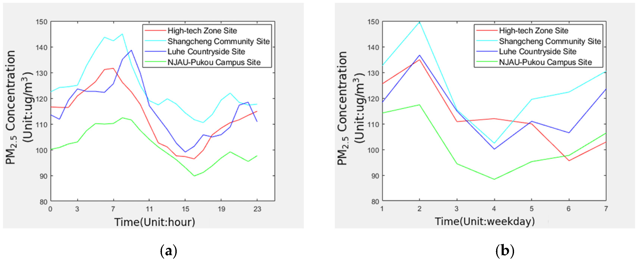
MATLAB software was used to average the preprocessed data according to 24 hours during a day and 7 days during a week. The resulting line figures are shown in Figure 4.
The Pearson correlation coefficient between any two different monitoring sites in is between 0.737 and 0.909. In Figure 5, the Pearson correlation coefficient is between 0.733 and 0.976. All of them showed a strong correlation, and it can be seen that the changing trend of PM2.5 concentration at the four monitoring sites are basically the same. In terms of temporal characteristics, PM2.5 concentration is the lowest at around 3–4 o’clock in the afternoon, and the highest concentration is around 7–8 o’clock in the morning during a day. Within a week, the PM2.5 concentration changed significantly, with a maximum difference of 47.18 ug/m3, which showed the highest on Tuesday. Except for High-tech Zone Site, which fell to the lowest on Saturday, the other three monitoring sites were the lowest on Thursday. Due to human activities, the value of PM2.5 will generally increase on Saturdays, Sundays, and Mondays. After life and work are stable, the value of PM2.5 will decrease. In terms of spatial characteristics, it can be seen from Table 2 that Shangcheng Community Site has the highest PM2.5 concentration and the largest fluctuation, NJAU-Pukou Campus Site is the lowest, and the change is the most stable, High-tech Zone Site and Luhe Countryside Site are at the same level. This is mainly due to Jiangbei New District focusing on the development of heavy and high-tech industry in recent years, resulting in increasingly serious air pollution. Compared with the other three monitoring sites, Shangcheng Community Site has more frequent staff movement, commercial activities, and more motor vehicle exhaust, which also lead to the increase of PM2.5 concentration. It shows that the air quality in Jiangbei New District has a strong correlation with the regional distribution.

3.2. Model Prediction Results

This research was conducted in the Python environment. The experimental equipment configuration is: Windows 10, Intel(R) Core(TM) i7-8750H CPU @ 2.20GHz (Intel, Santa Clara, CA, USA), 16GB memory, 1TB hard disk.
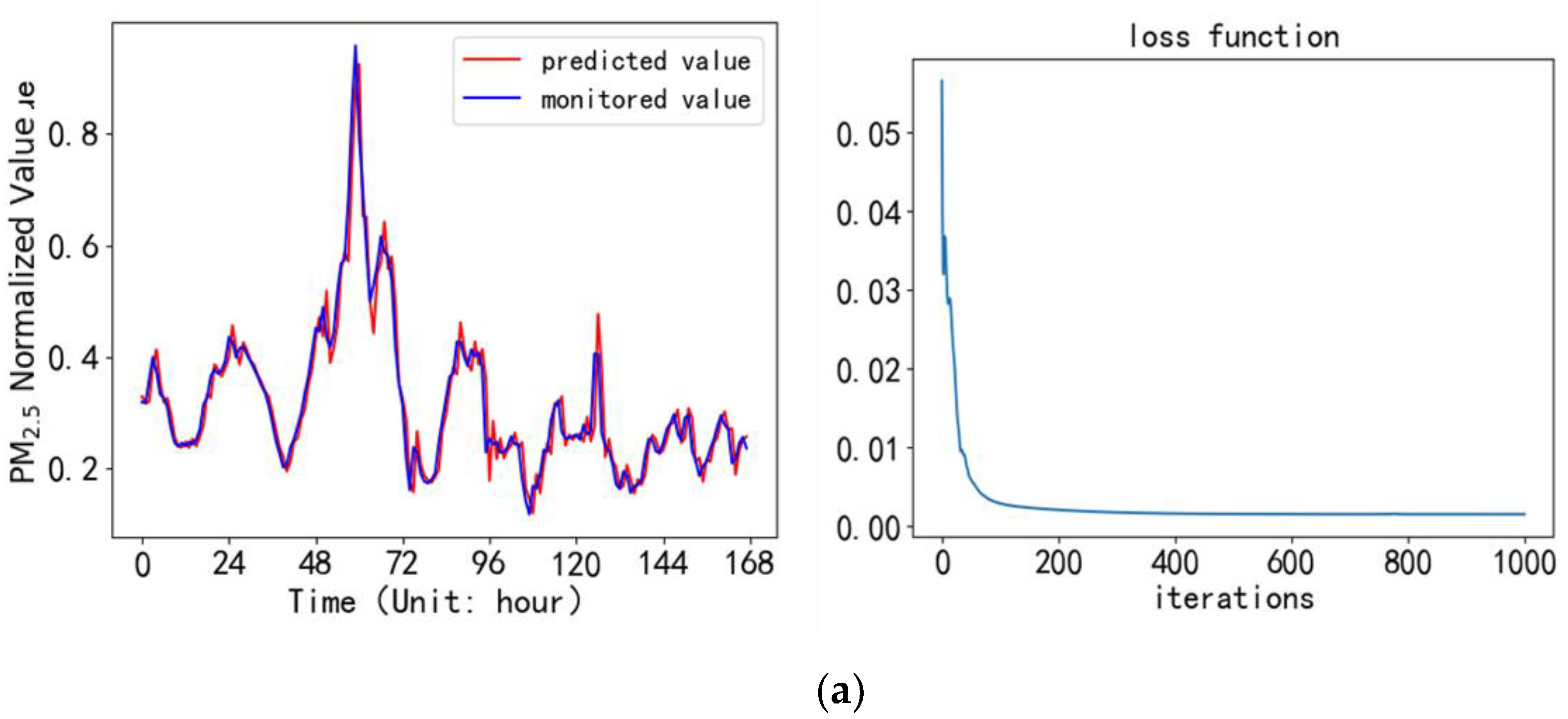
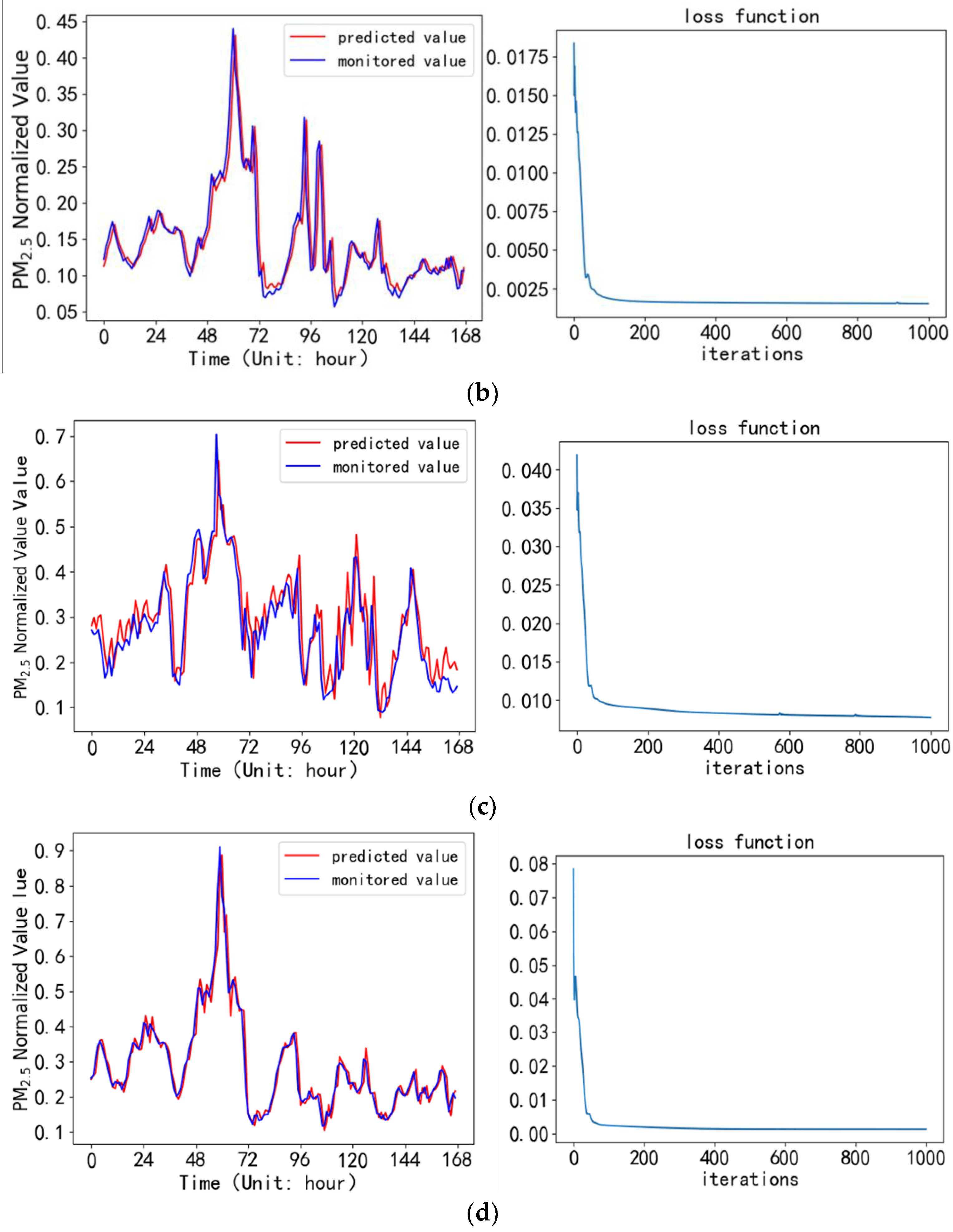
A PM2.5 concentration prediction model was established in the PyCharm compilation environment based on the above experimental environment configuration. The model used a test set to predict the PM2.5 hour average mass concentration in the next week for the four monitoring sites. The predicted values of the PM2.5 concentration are compared with the monitored value, and the loss functions during the iteration process were shown in Figure 5a–d.
It can be seen from Figure 5 that the predicted value of 168 hours in the next week is basically consistent with the monitored value. The model converges in the smallest gradient direction before 200 iterations, and the processing speed is fast. There is no overfitting in the model. After 1000 iterations, the loss rate output by the loss function is almost close to zero. Table 5 gives the prediction error and the correlation coefficient between the predicted value and the monitored value.
It can be seen from Table 5 that the correlation coefficient between the predicted value and the monitored value output by the PM2.5 concentration model based on GRU has reached more than 0.9. There is a strong correlation between the predicted value and the monitored value, and the MRE is around 10%. The results show that the PM2.5 concentration prediction model constructed by GRU network has good prediction performance. Among them, NJAU-Pukou Campus Site has the highest prediction accuracy, and Luhe Countryside Site has the lowest relative prediction accuracy. According to the spatiotemporal characteristics of PM2.5, the model performs better when predicting lower concentrations of PM2.5.
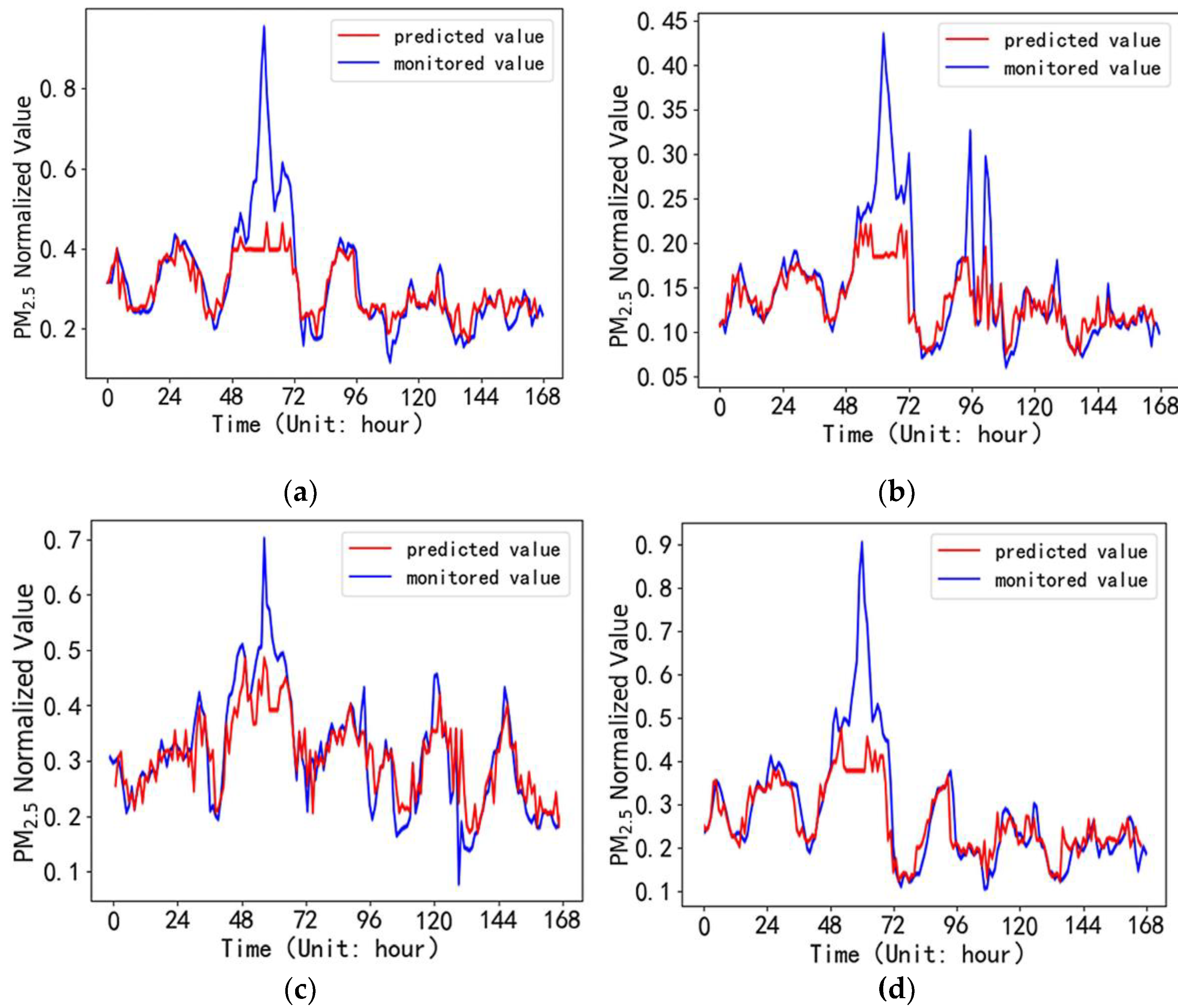
The SVR model used test set to predict the PM2.5 hour average mass concentration in the next week for the four monitoring sites. The predicted values of the PM2.5 concentration are compared with the monitored values, as shown in the results in Figure 6a–d.
It can be seen from Figure 6 that the predicted value of 168 hours in the next week is also basically consistent with the monitored value. However, it does not predict the sharp peak of the curve well. Table 6 gives the prediction error and the correlation coefficient between the predicted value and the monitored value for SVR model.
Compared with SVR model and some existing studies, such as LSTM [21], the correlation coefficient of GRU model reaches more than 0.9, but that of SVR model is only around 0.8. In addition, the MRE of GRU model is around 10%; however, that of SVR model is more than 20%. From this index, it can be seen that GRU deep learning model is more accurate in prediction and has great advantages in convergence speed, which can better fit the nonlinear problems in air quality prediction. Due to the complex causes of PM2.5 and pollutant concentration, it has a strong correlation with people’s life and production activities, etc. However, access to data regarding areas such as traffic and factory production is limited. In the next step, more relevant data need to be obtained to improve the accuracy of the model.

4. Conclusions

In order to analyze and predict air quality, four monitoring sites were arranged to collect PM2.5/PM10 concentration data, temperature, and humidity data in Jiangbei New District of Nanjing City, and an analysis of PM2.5 spatiotemporal characteristics was conducted. The concentrations of PM2.5 at the four monitoring sites showed the same trend, peaking around 7 a.m. and falling to the lowest around 4 p.m. during the day. During a week, PM2.5 concentrations reached their highest on Tuesday and, with the exception of the High-tech Zone site, which dropped to the lowest on Saturday, the other three monitoring sites all dropped to the lowest on Thursday. Among the four monitoring sites, Shangcheng Community Site had the highest concentration of PM2.5 with a large dispersion, while NJAU-Pukou Campus Site had the lowest concentration of PM2.5 with the most stable change. The GRU network prediction model for PM2.5 concentration was established to predict the hourly average mass concentration of PM2.5 at four monitoring sites. The results show that the predicted values are very close to the measured value. The Pearson correlation coefficient is greater than 0.9, which reflects the strong correlation between the two sites. MRE and RMSE are smaller, among which the prediction effect of Pukou Campus of Nanjing Agricultural University is the best, as the Pearson correlation coefficient is 0.970, MRE is 7.85, and RMSE is 9.6049. The experimental results show that the model has good prediction accuracy and generalization ability. The PM2.5 spatiotemporal characteristics and GRU model studied in this paper show the potential for analyzing and predicting urban air quality. It could be popularized in other cities and regions, as well as provide decision support for decision-makers on air pollution assessment, early warning, and treatment. It also could be applied to improve the environmental air quality and lay a theoretical foundation for better development of urban construction. At the same time, it can provide people with air quality forecasts, help people know the air quality situation in the future in advance, and take relevant preventive measures to reduce the impact of air pollution on their health.

Author Contributions

Conceptualization, Y.L. and X.Z.; Data curation, Z.Z., S.W. and Z.L.; Funding acquisition, Y.L. and X. Z.; Methodology, Y.L., Z.Z. and X.Z.; Project administration, X.Z.; Visualization, Z.Z., C.X. and Z.C.; Writing-original draft, Y.L., Z.Z., C.X., Z.C. and X.Z.; Writing-review & editing, X.Z.. All authors have read and agreed to the published version of the manuscript.

Funding

This research was funded by the Jiangsu Agriculture Science and Technology Innovation Fund, China (CX(21)3058), the Innovation Fund of Wuxi Vocational Institute of Commerce, China (KJXJ22508), and the University Student Entrepreneurship Training Program of Jiangsu, China (202112702008T).

Institutional Review Board Statement

Not applicable.

Informed Consent Statement

Not applicable.

Data Availability Statement

Not applicable.

Acknowledgments

The authors are grateful to Jie Zhang and Yuanyuan Song from Nanjing Agricultural University for their assistance, and thank all other participants for technical support.

Conflicts of Interest

The authors declare no conflict of interest.

References

  1. Ministry of Ecology and Environment of China. China’s Environmental State Communique. 2018. Available online: https://www.mee.gov.cn/xxgk2018/xxgk/xxgk15/201912/t20191231_754139.html (accessed on 15 July 2022).
  2. He, K.; Yang, F.; Ma, Y.; Zhang, Q.; Yao, X.; Chan, C.K.; Cadle, S.; Chan, T.; Mulawa, P. The characteristics of PM2.5 in Beijing, China. Atmos. Environ. 2001, 35, 4959–4970. [Google Scholar] [CrossRef]
  3. Pui, D.Y.H.; Chen, S.C.; Zuo, Z. PM2.5 in China: Measurements, sources, visibility and health effects, and mitigation. Particuology 2014, 13, 1–26. [Google Scholar] [CrossRef]
  4. Kampa, M.; Castanas, E. Human health effects of air pollution. Environ. Pollut. 2008, 151, 362–367. [Google Scholar] [CrossRef] [PubMed]
  5. Dockery, D. Effects of inhalable particles on respiratory health of children. Am. Rev. Respir. Dis. 1989, 139, 587–594. [Google Scholar] [CrossRef] [PubMed]
  6. Zhao, C.; Wang, Y.; Su, Z.; Pu, W.; Niu, M.; Song, S.; Wei, L.; Ding, Y.; Xu, L.; Tian, M.; et al. Respiratory exposure to PM2.5 soluble extract disrupts mucosal barrier function and promotes the development of experimental asthma. Sci. Total Environ. 2020, 730, 139–145. [Google Scholar] [CrossRef]
  7. Zhu, G.; Hu, W.; Liu, Y.; Cao, J.; Ma, Z.; Deng, Y.; Sabel, C.E.; Wang, H. Health burdens of ambient PM2.5 pollution across Chinese cities during 2006–2015. J. Environ. Manag. 2019, 243, 250–256. [Google Scholar] [CrossRef]
  8. Ding, S.; Xu, N.; Ye, J.; Ye, J.; Zhou, W.; Zhang, X. Estimating Chinese energy-related CO2 emissions by employing a novel discrete grey prediction model. J. Clean. Prod. 2020, 259, 120793. [Google Scholar] [CrossRef]
  9. Pozza, S.A.; Lima, E.P. Time series analysis of PM2.5 and PM10-2.5 mass concentration in the city of Sao Carlos, Brazil. Int. J. Environ. Pollut. 2010, 41, 90–108. [Google Scholar] [CrossRef]
  10. Dimitriou, K.; Kassomenos, P. A study on the reconstitution of daily PM10 and PM2.5 levels in Paris with a multivariate linear regression model. Atmos. Environ. 2014, 98, 648–654. [Google Scholar] [CrossRef]
  11. Christakos, G.; Serre, M.L. BME analysis of spatiotemporal particulate matter distributions in North Carolina. Atmos. Environ. 2000, 34, 3393–3406. [Google Scholar] [CrossRef]
  12. Grivas, G.; Chaloulakou, A. Artificial neural network models for prediction of PM10 hourly concentrations, in the Greater Area of Athens, Greece. Atmos. Environ. 2006, 40, 1216–1229. [Google Scholar] [CrossRef]
  13. Perez, P.; Gramsch, E. Forecasting hourly PM2.5 in Santiago de Chile with emphasis on night episodes. Atmos. Environ. 2016, 124, 22–27. [Google Scholar] [CrossRef]
  14. Chen, Y.G. Prediction algorithm of PM2.5 mass concentration based on adaptive BP neural network. Computing 2018, 100, 825–838. [Google Scholar] [CrossRef]
  15. Prakash, A.; Kumar, U.; Kumar, K.; Jain, V.K. A wavelet-based neural network model to predict ambient air pollutants’ concentration. Environ. Modeling Assess. 2011, 16, 503–517. [Google Scholar] [CrossRef]
  16. Huang, C.J.; Kuo, P.H. A deep CNN-LSTM model for particulate matter (PM2.5) forecasting in smart cities. Sensors 2018, 18, 2220. [Google Scholar] [CrossRef] [PubMed]
  17. Cho, K.; Merrienboer, B.V.; Gulcehre, C.; Badanau, D.; Bougares, F.; Schwenk, H.; Bengio, Y. Learning phrase representations using RNN encoder-decoder for statistical machine translation. arXiv 2014, arXiv:1406.1078. [Google Scholar]
  18. Hochreiter, S.; Schmidhuber, J. Long short-term memory. Neural Computation 1997, 9, 1735–1780. [Google Scholar] [CrossRef]
  19. Gers, F.A.; Schmidhuber, J.; Cummins, F. Learning to forget continual prediction with LSTM. Neural Comput. 2000, 12, 2451–2471. [Google Scholar] [CrossRef]
  20. Zou, X.; Qian, Y.; Zhang, S. Spatiotemporal variations of PM2.5 concentration and relationship with other criteria pollutants in Nanjing, China. Nat. Environ. Pollut. Technol. 2018, 17, 499–505. [Google Scholar]
  21. Zhang, S.; Lin, M.; Zou, X.; Steven, S.; Zhang, W.; Zhang, X.; Guo, Z. LSTM-based air quality predicted model for large cities in China. Nat. Environ. Pollut. Technol. 2020, 19, 229–236. [Google Scholar]
  22. Ji, H.; Wang, Q.; Yu, Y.; Lu, Y. How have the characteristics of air quality in a typical large Chinese city changed between 2011 and 2017. Air Qual. Atmos. Health 2019, 12, 401–410. [Google Scholar] [CrossRef]
  23. Kingma, D.; Ba, J. Adam: A method for stochastic optimization. arXiv 2015, arXiv:1412.6980v9, 1–15. [Google Scholar]
  24. Bottou, L. Large-scale machine learning with stochastic gradient descent. In Proceedings of the 19th International Conference on Computational Statistics (COMPSTAT'2010), Paris, France, 22–27 August 2010; pp. 177–186. [Google Scholar]
  25. Ketkar, N. Introduction to PyTorch; Apress: Berkeley, CA, USA, 2017; Chapter 12; pp. 195–208. [Google Scholar]
  26. Quang, D.; Guan, Y.; Parker, S.C.J. YAMDA: Thousandfold speedup of EM-based motif discovery using deep learning libraries and GPU. Bioinformatics 2018, 34, 3578–3580. [Google Scholar] [CrossRef] [PubMed]
  27. Sedgwick, P. Pearson’s correlation coefficient. BMJ 2012, 345, e4483. [Google Scholar] [CrossRef] [Green Version]
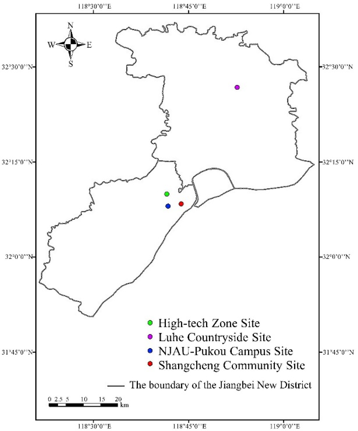
Figure 1. Spatial distribution of four ambient air quality monitoring sites in Jiangbei New District.
Atmosphere 13 01542 g001
Figure 2. Air quality transmitter and temperature & humidity transmitter.
Atmosphere 13 01542 g002
Figure 3. GRU model structure.
Atmosphere 13 01542 g003
Figure 4. The resulting line figures of averaging the preprocessed data using MATLAB software: (a) PM2.5 hourly average concentration change line; (b) PM2.5 daily average concentration change line.
Atmosphere 13 01542 g004
Figure 5. Comparison between predicted values and monitored values by GRU model in the coming week, and the figures of loss function: (a) High-tech Zone Site; (b) Shangcheng Community Site; (c) Luhe Countryside Site; (d) NJAU-Pukou Campus Site.
Atmosphere 13 01542 g005aAtmosphere 13 01542 g005b
Figure 6. Comparison between predicted values and monitored values by SVR model in the coming week: (a) High-tech Zone Site; (b) Shangcheng Community Site; (c) Liuhe Countryside Site; (d) NJAU-Pukou Campus Site.
Atmosphere 13 01542 g006
Table 1. Some parameters of Jianda Renke Transmitter.
IndexAccuracyResolutionRange
PM2.5 ± 10 10~1000(ug/m3)
PM10 ± 10 10~1000(ug/m3)
Temperature ± 0.5 0.1−40~+80 (°C)
Relative Humidity ± 3 0.10~100 (%)
Table 2. Statistical analysis results of PM2.5 concentration data.
SiteData VolumeMaximum
Value
Minimum
Value
Mean
Value
Standard
Deviation
High-tech Zone Site62,084453511361
Shangcheng Community Site83,872499312476
Luhe Community Site65,006499911665
NJAU-Pukou Campus Site83,055397310159
Table 3. Air quality grades and human activities affected.
Air Quality GradesAir Pollution Index (API)Impact of Human Life
Excellent0–50Normal activities
Good51–100Normal activities
Light pollution101–200Susceptible populations have mild exacerbations, and healthy people experience irritation symptoms.
Moderate pollution201–300Symptoms of heart disease and lung disease patients are significantly increased, and healthy people’s exercise tolerance decreases.
Severe pollutionMore than 301Healthy people have obvious symptoms and certain diseases.
Table 4. Correspondence between | r xy | and correlation strength.
| r xy | .  
Correlation Strength
0.8–1.0Highly relevant
0.6–0.8Strong correlation
0.4–0.6Moderate correlation
0.2–0.4Weak correlation
0.0–0.2Very weak correlation or no correlation
Table 5. Evaluation results of the four monitoring sites for GRU model.
SiteMRE (%)RMSE (ug/m3)Pearson Correlation Coefficient
High-tech Zone Site9.0313.54840.958
Shangcheng Community Site11.1016.93160.928
Luhe Countryside Site11.1917.03780.907
NJAU-Pukou Campus Site7.859.60490.970
Table 6. Evaluation results of the four monitoring sites for SVR model.
SiteMRE (%)RMSE (ug/m3)Pearson Correlation Coefficient
High-tech Zone Site12.5130.23630.805
Shangcheng Community Site32.9413.58000.761
Luhe Countryside Site20.0718.06910.872
NJAU-Pukou Campus Site24.5612.71000.837
Publisher’s Note: MDPI stays neutral with regard to jurisdictional claims in published maps and institutional affiliations.