Article

Sub-Seasonal Prediction of Sea-Gale Processes in the Yangtze River Estuary of China

1
Shanghai Marine Meteorological Center, Shanghai Meteorological Service, Shanghai 200030, China
2
Key Laboratory of Cities’ Mitigation and Adaptation to Climate Change in Shanghai, Shanghai Regional Climate Center, Shanghai 200030, China
3
Changshu Meteorological Service, Jiangsu Meteorological Service, Suzhou 215516, China
*
Author to whom correspondence should be addressed.
Atmosphere 2023, 14(4), 682; https://doi.org/10.3390/atmos14040682
Submission received: 26 February 2023 / Revised: 31 March 2023 / Accepted: 2 April 2023 / Published: 5 April 2023

Abstract

:
The sea-gale process (SGP) is a significant and disastrous weather event for the marine industry. However, the sub-seasonal predictability of SGP remains unclear. In this study, we investigate the influence of low-frequency oscillation on SGP in the Yangtze River estuary from November to April, and its implications for sub-seasonal prediction. We noted that SGPs have a close relationship with the 10~30 day low-frequency component of the 10-m wind speed in the Yangtze River estuary, and typically occur during the peak phase of the low-frequency oscillation. The 10~30 day low-frequency oscillation of 10-m wind was found to be linked to the eastward propagation of extratropical Rossby waves from the North Atlantic across Europe to East Asia. This Rossby wave leads to the low-frequency oscillation of the Siberian high pressure and Japan Sea low pressure, which is indicative of the 10~30 day low-frequency oscillations of the 10-m wind speed in the Yangtze River Estuary. A sea-gale process index (SGPI) was constructed based on the low-frequency oscillation of the Siberian high and the Japan Sea low in order to predict SGPs at the sub-seasonal time scale. Hindcast and real-time forecasts showed that 2/3 of SGPs can be predicted with a leading time of 10~30 days, and that good sub-seasonal predictions of SGPs are connected with strong low-frequency oscillations at the initial forecast time. Therefore, SGPI can be adopted for the sub-seasonal prediction of SGPs in the Yangtze River Estuary.

1. Introduction

Accurately forecasting weather beyond ‘weather’ time scales (up to 10 days) can offer significant socio-economic value by enabling effective management and planning for changes in weather and climate [1,2]. Sub-seasonal predictions, which refer to predictions beyond 10 days and up to a season, bridge the forecasting ‘gap’ between the conventional weather forecast and short-range climate prediction [3]. Sea gales are a major disastrous weather event for the marine industry, where sub-seasonal prediction can help to reduce marine accidents and their related economic cost for offshore operations more than 10 days in advance. Accurate wind-speed forecasts in the sub-seasonal timescale are also needed for the growing marine wind-energy industries [4]. To the authors’ knowledge, this has yet to be implemented.
Skillful sub-seasonal prediction is challenging because the timescale is both too long for the initial conditions to persist and too short for the boundary conditions to have a significant impact [2,5,6,7]. The development and implementation of sub-seasonal prediction have become essential research areas for operational developments in both weather forecasting and climate prediction in the last two decades [8]. Recent studies have shown that the Madden-Julian oscillation (MJO) [9,10] is the most important source of predictability at the sub-seasonal timescale [11,12,13,14,15], as MJO is the dominant mode of atmospheric variability in the tropics. In addition to the MJO, low-frequency oscillations, including bi-weekly and 30–60-day oscillations, are widespread in the global atmosphere [16,17]. These oscillations have been found to be closely associated with heavy rainfall, heatwave, cold surges, and other weather phenomena in the east Asian monsoon region [18,19,20,21,22]. However, the relationship between sea gales and atmospheric low-frequency oscillations is still unclear.
Forecasts at the sub-seasonal timescale have been greatly improved in recent years [23,24]. Currently, sub-seasonal forecasting methods mainly fall into two categories: dynamic models; [25] and physical statistics [26]. Dynamic models have been widely used in sub-seasonal forecasts since the Sub-seasonal to Seasonal (S2S) Project created an extensive database containing sub-seasonal (up to 60 days) forecasts and reforecasts from 11 operational and research centers [3]. In recent years, several studies have assessed the skill of sub-seasonal forecasts of wind. Lynch et al. [27] evaluated the skill of the European Centre for Medium-Range Weather Forecasts’ (ECMWF) extended-range forecasts and found statistically significant skill in predicting weekly mean wind speeds in Europe at leading times of 14–20 days. Soret et al. [28] also found that 10-m wind speed forecasted in S2S model exhibited predictability in advance of some weeks or months in the North Sea in Europe. Goutham et al. [7] further revealed that the sub-seasonal forecast skills of 100-m wind speed depend on the choice of the geographical domain and the forecast attributes, with some results showing skillful predictions beyond two weeks, thereby encouraging their implementation in operational decision-making.
Meanwhile, the low-frequency oscillation, especially MJO, has been utilized to investigate the predictability of sub-seasonal precipitation, temperature, and other related variables [14,15,19,29,30]. Lledo and Doblas-Reyes [31] assessed the impact of strong MJO events on 10-m wind speed over Europe and concluded that MJO can be utilized to develop a hybrid statistical–dynamical model to enhance the prediction of 10-m wind speed. Furthermore, teleconnection patterns, including the North Atlantic Oscillation, East Atlantic, and Scandinavian patterns, are important sources of predictability of winds in the Iberian Peninsula [32]. Hence, the sub-seasonal predictability of wind may be affected by global signals in Europe. In China, the spatial–temporal projection model (STPM) has exhibited high skill in predicting rainfall, temperature anomalies, and extreme events including floods, heatwaves, and cold surges with a leading time of 10 to 30 days, by filtering out weather noise [33,34,35,36]. However, the sub-seasonal predictability of SGPs in East Asia remains unclear due to the limited number of historical observations at sea and the rare methods of sub-seasonal forecasting of SGPs.
In this study, we investigated the sub-seasonal variability and statistical sub-seasonal prediction model of SGPs using observational wind data from five buoy stations in the Yangtze River Estuary in China. We chose the Yangtze River Estuary as it is a key location with many large marine industry enterprises in China. We focused on the winter half-year period from November to April as maritime accidents are much more frequent during the winter season than the summer season [37]. Section 2 briefly outlines the data sources and methodologies used in this study. In Section 3, we analyze the characteristics of the sub-seasonal variability of SGPs in the winter half-year in the Yangtze River estuary. And we discuss the intra-seasonal evolution of the atmospheric circulation associated with the SGPs and establish a statistical model for sub-seasonal prediction of SGPs, and its predictability is then analyzed. Finally, the summaries and discussions are presented in Section 4.

2. Data and Methods

The observational 10-m wind-speed data were collected every 2 min from October 2011 to May 2022 from five buoy stations located in the Yangtze River Estuary, and were provided by the Shanghai Marine Meteorological Center and the Institute of Oceanology, Chinese Academy of Sciences. Figure 1 depicts the geographical distribution of the five buoy stations, i.e., the South Yangtze River Estuary Buoy, Yangtze River Estuary Buoy, Shanghai Meteorological No. 1 Buoy, Ocean Reef Buoy, and Huangze Ocean Buoy.
Daily surface pressure, geopotential height, and wind fields from NCEP/DOE Reanalysis II [38] “https://psl.noaa.gov/data/gridded/data.ncep.reanalysis2.html (accessed on 30 May 2022)” were used for the investigation of the atmospheric evolution associated with the sub-seasonal variability of sea gales.
The wind-speed data were quality controlled in order to ensure the homogeneity of the wind speed recorders. By following the existing operational quality control techniques of observational data [39], the quality-control scheme of the observational wind speeds includes four steps: (1) Integrity check, i.e., lack of observational records due to station failure or instrument failure; (2) Internal consistency check, which excludes the following two circumstances: wind direction > 360°or 0°, wind speed is zero, and wind direction 0°; (3) Climate extreme value check, which primarily consists of climate limit value check and station extreme value check. Generally, data with wind speed > 75 m/s are regarded as anomalies. Meanwhile, station extremes include the maximum and minimum values that have ever occurred in the history of a station. The threshold of extreme value is adjusted by enhancement or decrease of 5 m/s based on the extreme values in the corresponding months considering new extremes may occur; and (4) Time consistency check of instrument failures when the wind speed measurements remain consistent in an hour. The results of the data quality control show that the wind speed observation every 2 min originating from the five buoy stations is reliable and can be used for further research. The daily average (from 20:00 to 20:00 Beijing time) wind speeds were then calculated and further used in this study.
The statistical methods used include (1) Percentile method [40]: the daily wind speeds from the five buoy stations were ranked from lowest to highest during the winter half-years (November to April of the next year, same hereafter) of 2011–2021. The statistical percentile was then calculated, and the 85th percentile of the wind speed is used as the threshold for strong sea gales; (2) Wavelet analysis method [41]: a method to obtain various “periodic” signals by simultaneous decomposition of time series in the time and frequency domains based on a variable-scale wavelet basis. In this paper, it was applied to determine the period of SGPs in the Yangtze estuary during the winter half-year. It should be noted that before the wavelet analysis of the daily wind data, a 9-point sliding average is first performed to filter out the effects of high-frequency weather scales; and (3) Butterworth filtering [42]: a filtering method that obtains the intermediate frequency signals between the period bands by filtering out high- and low-frequency signals. The Butterworth filtering method has the advantages of almost no loss of input length and fast convergence. In this paper, Butterworth filtering was used to extract the intra-month (10~30 day) low-frequency component associated with SGPs.
The three-dimensional wave activity flux W (Equation (1)) was also calculated to quantitatively diagnose the Rossby wave energy dispersion characteristics [43].
W = 1 2 | V | ( u ¯ ( ψ x 2 ψ ψ xx ) + v ¯ ( ψ x ψ y ψ ψ xy ) u ¯ ( ψ x ψ y ψ ψ xy ) + v ¯ ( ψ y 2 ψ ψ yy ) f 2 R σ / p [ u ¯ ( ψ x ψ p ψ ψ xp ) + v ¯ ( ψ y ψ p ψ ψ yp ) ] )
where  | V |  is the horizontal wind speed at 200 hPa,  σ = R T ¯ C p p d T ¯ dp  is the atmospheric stability parameter,  C p  is the constant pressure specific volume,    u ¯ ,   v ¯ ,   T ¯  are the climatological latitudinal wind, longitudinal wind and temperature respectively, R is the ideal air constant, f is the ground rotation parameter, p is the barometric pressure, and  ψ  is the disturbance flow function.
To identify large-scale persistent SGPs in the Yangtze River estuary, the following three steps are used: (1) Determination of a strong sea-gale day: the daily wind speed exceeding the 85th percentile threshold in the winter half-year is used as the criterion of strong sea gales. If at least two of the five stations have strong sea gales on a given day, it is considered a strong sea-gale day; (2) Determination of an SGP: a process with continuous strong sea-gale days or spaced only one day. (3) Determination of a large-scale persistent SGP: the duration of a SGP ≥ 3 days. Thus, both the spatial and temporal continuity are considered in the identification of SGPs. The above statistics on SGPs are basically consistent with the current meteorological operational regulations.

3. Results

3.1. Characteristics of the Low-Frequency Oscillations of SGPs in Winter Half-Years

According to the statistics of SGPs during 2011–2022, 23 SGPs with an average (maximum) duration of four days (six days) occurred in the winter half-years in the Yangtze River estuary. The frequency of SGPs was significantly correlated with the average wind speed in winter half-years with a correlation coefficient of 0.61 above 0.01 significance level. Therefore, SGPs contributed significantly to the windy weather in winter half-years, thus highlighting the significance of conducting sub-seasonal forecasting of SGPs.
Figure 2 shows the wavelet analysis of the daily 10-m wind speed along the Yangtze River Estuary during the winter half-years of 2011–2017. It can be seen that from the viewpoint of climatological intra-seasonal variability, the wind in the Yangtze estuary has a significant 10~30 day low-frequency oscillation cycle in winter half-years.
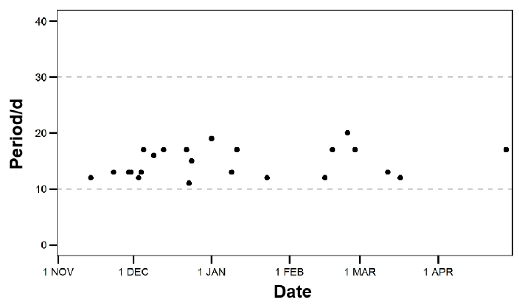
After analyzing each SGP, it was found that they usually occur during the peak stage of the low-frequency oscillation of the 10-m wind speed. The significant period distribution of the low-frequency oscillations of daily wind speeds corresponding to SGPs in the Yangtze River Estuary is further shown in Figure 3. It shows that 65% of SGPs took place at the peak phase of 10~30 day low-frequency oscillation. 23 SGPs were detected in winter half-years of 2011–2017, with an average frequency of three times each year and an average duration of four days during the peak phase of the 10~30-day oscillation.
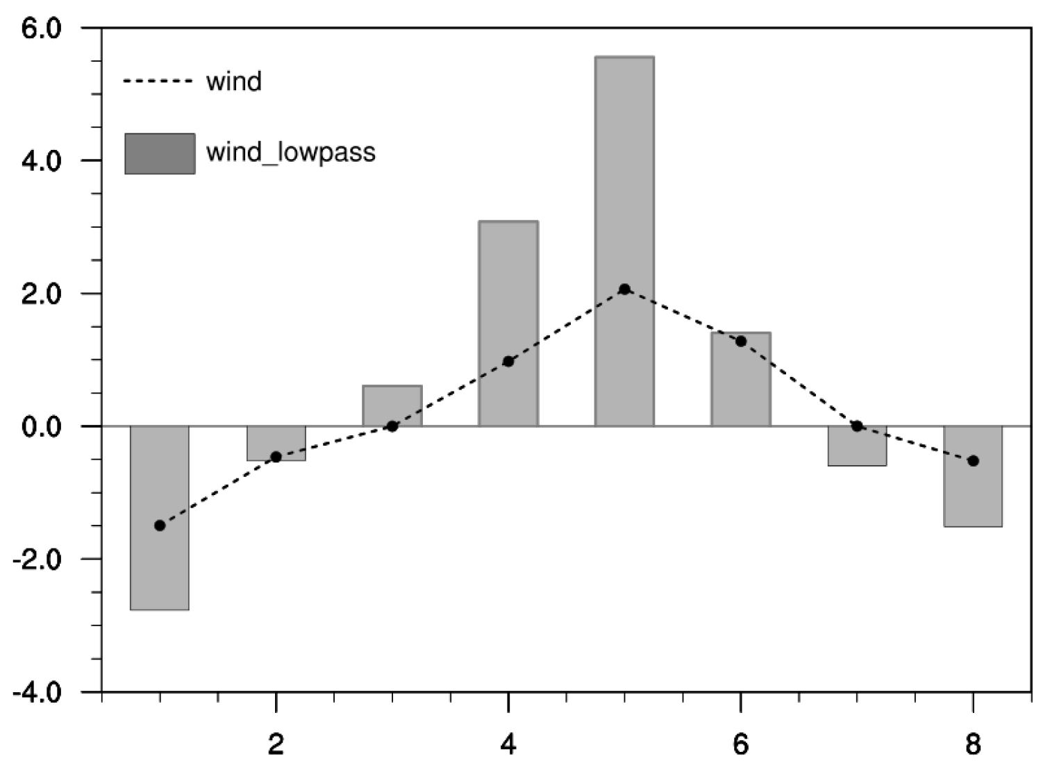
In order to investigate the sub-seasonal variability of SGPs, components with a 10~30-day period were filtered from the daily 10-m wind speed in the Yangtze Estuary during the winter half-years of 2011–2021. Each cycle of the 10~30 day low-frequency variation was separated into eight phases (Figure 4). As shown in Figure 4, phases 1 and 5 represent the trough and peak phase of the 10~30 day low-frequency cycle, respectively. The variation of the 10~30 day low-frequency component is in good agreement with the variation of the actual wind speed, exhibiting an increasing trend from phase 1 to 5 and a decreasing trend from phases 5 to 8. In other words, phases 1 and 5 correspond to the valley (peak) stage of the actual wind speed and its 10~30 day low-frequency component respectively. SGPs usually happen in phases 4–6 of the 10~30 day low-frequency oscillation, when the actual wind speed is notably positive anomalous. Therefore, SGPs are in close connection with the 10~30 day low-frequency oscillations due to their agreement of the intra-seasonal evolution.

3.2. Characteristics of Circulation Background of SGPs

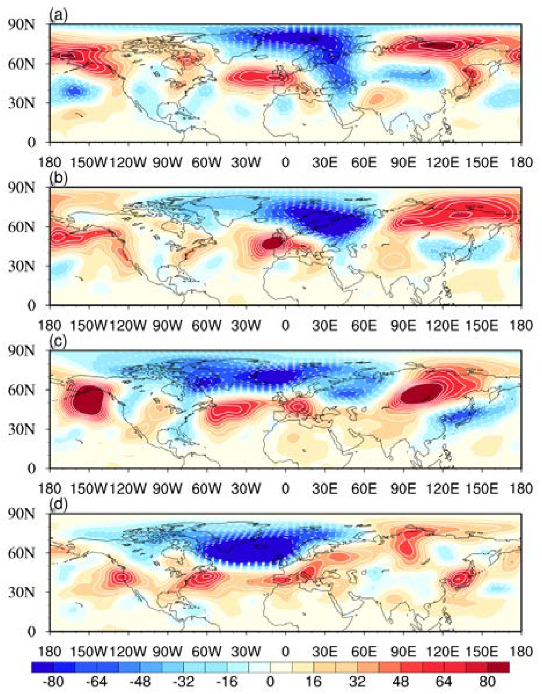
Figure 5 shows the composite anomalous geopotential height at 500 hPa during different phases of the 10~30 day low-frequency oscillations of the 10-m wind speed associated with SGPs. As shown in Figure 5a (phase 1), a distinct trough locates along 30° E over the mid-high latitudes of Asia. Subsequently, the trough eastward moves to 60° E at phase 3 (Figure 5b), while a negative anomalous geopotential height center appears along 90°–120° E in northeast Asia. The anomalous circulation distribution further moves eastward from phase 3 to phase 5. At phase 5 (Figure 5c), the anomalous circulation with two troughs and one ridge is located over the middle and high latitudes of Asia-Europe, with the high-pressure ridge centered on the Ural Mountains and low-pressure troughs on either side, which is consistent with the distribution of the east–west anomalous pressure field and favor to the cold-air intrusion to the Yangtze River Estuary.
The composite anomalous sea-level pressure fields at different phases of the 10~30 day low-frequency oscillation of wind speed associated with SGPs (Figure not shown) were also analyzed. The distribution of east low and west high also exhibits over the mid-high latitudes of East Asia at peak phases of the 10~30 day low-frequency oscillations of the 10-m wind speed, which is similar with the geopotential height anomaly field at 500 hPa. This suggests that SGPs took place in the quasi-barotropic circulation condition background.

3.3. Evolution of the 10~30 Day Low-Frequency Circulation of SGPs

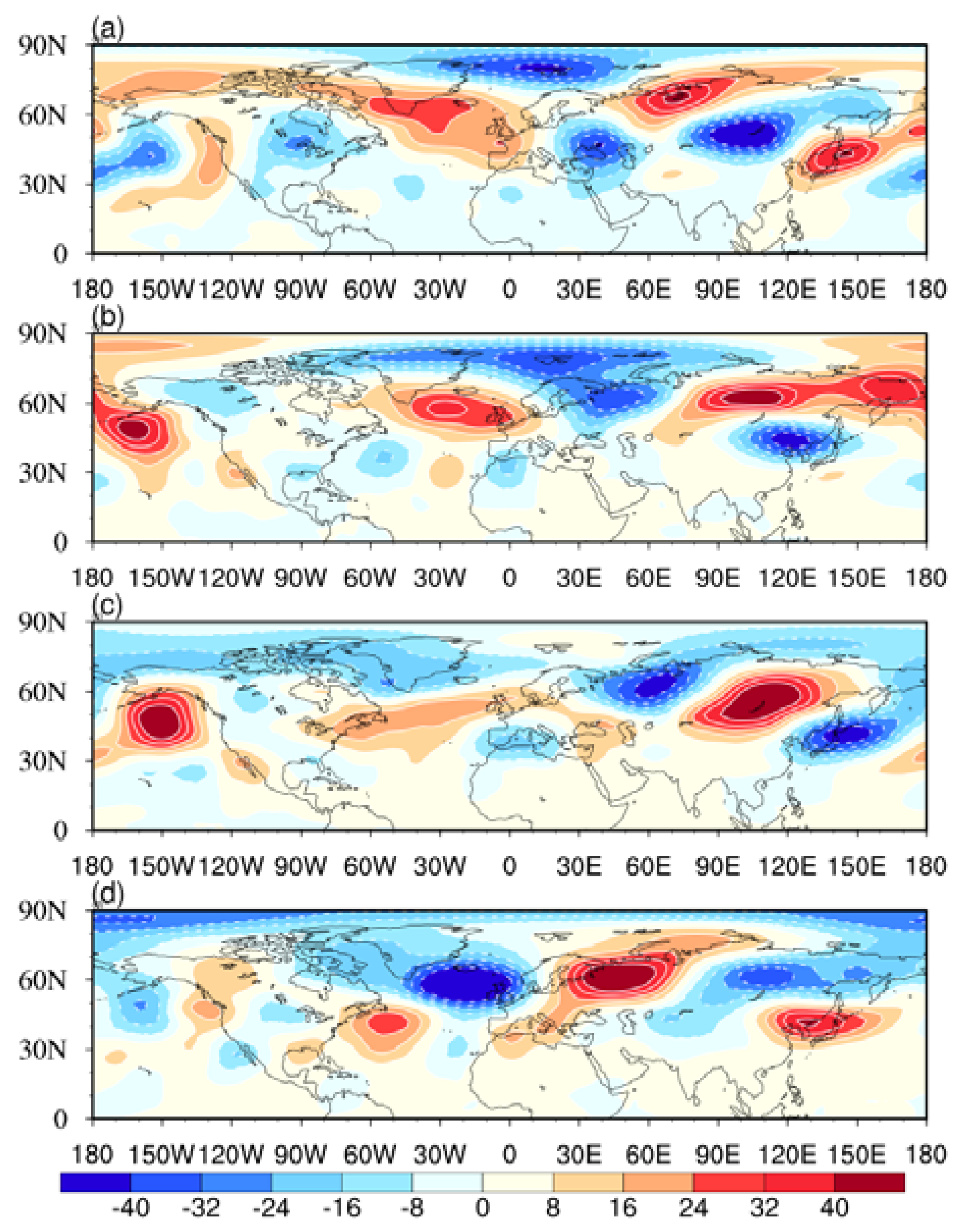
Considering the quasi-barotropic structure of circulation associated with SGPs in the low and middle level atmosphere, the 10~30 day filtered geopotential height at 500 hPa (Figure 6) was further adopted to investigate the sub-seasonal circulation evolution of SGPs. As can be seen in Figure 6a, a significant low-frequency positive value center is located in the area from 30° E to 60° E over the mid-high latitudes of Asia at phase 1, and moves eastward to the region of 90°–120° E at phase 3 (Figure 6b), while a low-frequency negative value center appears in 20°–50° E over the high latitudes of Asia at phase 5 (Figure 6c), thus a “+” “−” “+” “−” distribution of low-frequency geopotential height forms over the middle and high latitudes of Asia-European continent. At phase 7 (Figure 6d), the positive value center originally located at 90°–120° E is replaced by a negative value center, while the negative value centers originally located at 30°–50° N and 130°–160° E are replaced by positive value centers.
To examine the physical processes associated with the low-frequency circulation evolution described above, we further investigated the evolution of the wave activity flux at 200 hPa (Figure 7). As seen in Figure 7, the Rossby wave train from the north Atlantic travels eastward through the Eurasian continent along two branches of the wave guide. For the north branch, the wave train propagates northeastward to the polar channel and then southeastward to the Asian continent, resulting in the negative (positive) flux center over Asia-European high latitudes (northeast Asia) at phase 1 (Figure 7a) favoring the decreasing (enhancement) of wind speed over east China to its adjacent sea. The other southern branch of the wave train moves from the Black Sea to the Caspian Sea in the southeast at phase 1, then propagates eastward to the southern edge of the plateau and combines with the north branch wave train at phase 5 (Figure 7c), which strengthens the enhancement of the wind speed over east China to its adjacent sea. Therefore, the sub-seasonal evolutions of the low-frequency circulation associated with SGPs are impacted by the propagations of the wave train from the north Atlantic to northeast Asia via both the polar and the subtropical channels.

3.4. Sub-Seasonal Forecast Experiments of SGPs

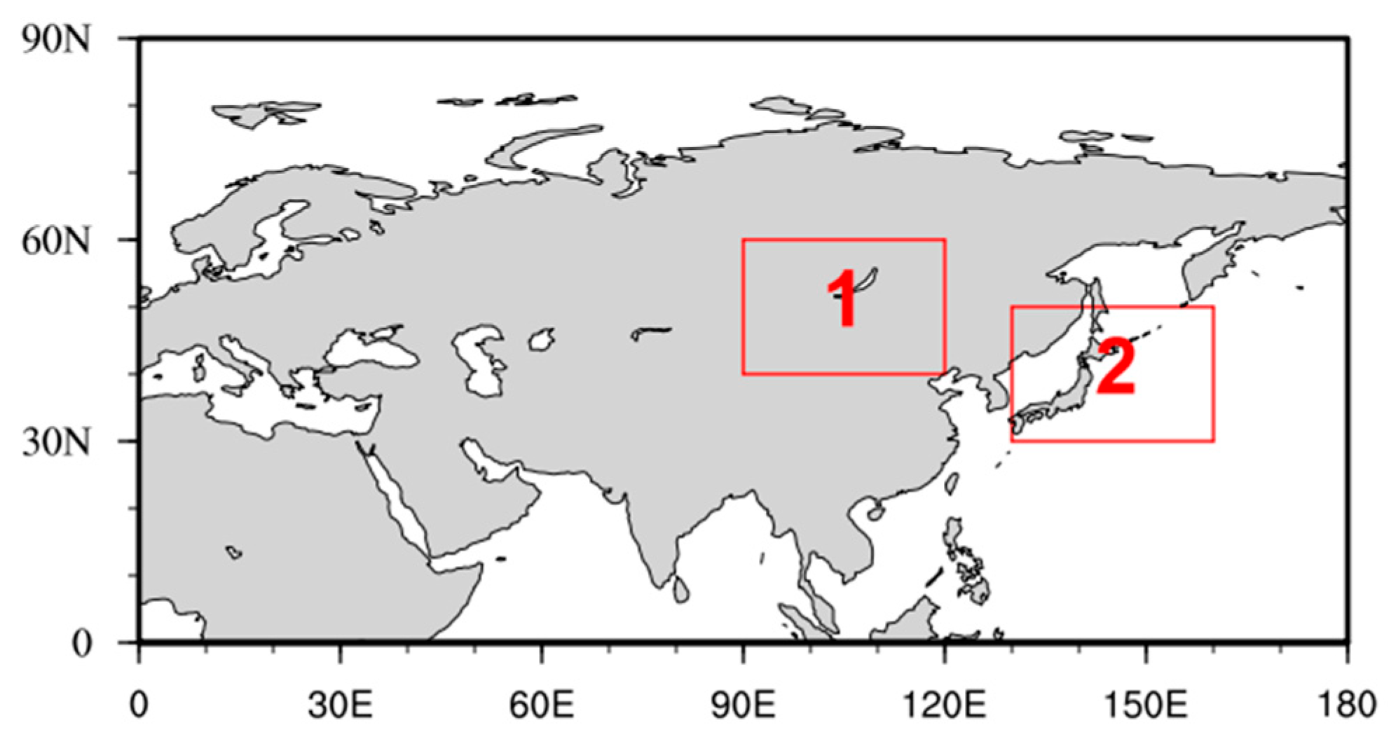
Low-frequency oscillations are an important means for sub-seasonal forecasts. As SGPs in the Yangtze River Estuary during winter half-years are mainly influenced by a 10~30 day low-frequency oscillation, the key regions (Figure 8) of the 10~30 day low-frequency oscillation of circulation at 500 hPa were chosen to design the index of sub-seasonal forecasts of SGPs. As shown in Figure 8, the key regions also corresponded to the activity centers of Rossby wave train over the high latitudes in Asia. The difference of the low-frequency geopotential height components between key region 1 (40°–60° N, 90°–120° E) and key region 2 (30°–50° N, 130°–160° E) was adopted to construct the SGPI index, which is calculated as follows:
SGPI = H ¯ 1 ' H ¯ 2 '
where “′”, “¯”, “1” and “2” indicate the 10~30 day filtered component, regional average, key region 1 and key region 2, respectively. Further analysis suggested that the peak of SGPI evolution agrees well with the fifth phase of the low-frequency oscillation of the wind speed associated with SGPs. In other words, the SGPI index can be used for sub-seasonal forecasting of SGPs.
SGPI was further adopted to forecast SGPs at the sub-seasonal time scale. For the initial forecast day, SGPI was computed for the previous 60 days. The corresponding SGPI evolution was extrapolated to determine the occurrence time of the subsequent peaks of SGPI evolution in the next 10~30 days. Thus, the extrapolation was based on the significant period of SGPI evolution. Then, the peak time was predicted as the occurrence time of an SGP. The following criteria were established to quantitatively evaluate the performance of the sub-seasonal forecast of SGPs: if the forecasted SGP overlaps with the observation or adjoins by only one day, the forecast is considered correct (score 100). Otherwise, it is incorrect (score 0). By taking the sub-seasonal forecast at the 10th day of every month from November 2011 to April 2022 as an example, the performance of the sub-seasonal forecast using SGPI is shown in Figure 9. In comparison with the observations, 25 forecasts were accurate, and the average forecast score was 64. Therefore, about two thirds of the SGPs can be predicted using SGPI index with a leading time of 10–30 days. Comparatively, the sub-seasonal forecast performance during November-December was better than March–April. The forecast performance also showed inter-annual variability, with the best performance in 2018.
Figure 10 further shows a good fit relationship between the sub-seasonal hindcast/forecast scores of SGPs and SGPI strength represented by the standard deviation of SGPI during the 30 days before the initial forecast time. The correlation coefficient is 0.73 above 0.01 significance level. For example, the score is highest (lowest) when the standard deviation is biggest (smallest) in 2018 (2017). Therefore, the intra-seasonal or interannual variability of the sub-seasonal forecast performance is positively correlated with the amplitude of SGPI. In other words, the forecast performance is modulated by the strength of the 10~30 day low-frequency oscillation at the initial time.

4. Discussion and Conclusions

Sub-seasonal prediction of sea-gale processes (SGPs) is crucial for mitigating natural disasters and managing marine resources. In this work, by focusing on the Yangtze estuary in winter half-years, the relationship between SGPs and low-frequency oscillations and its relating sub-seasonal prediction were analyzed. The conclusions are below:
The 10~30 day low-frequency oscillations are closely associated with SGPs, according to the variance contribution of the 10~30 day low-frequency wind component and its correlation with the actual 10m wind variation. The climatic daily variation of 10-m wind speed in the Yangtze Estuary exhibits a significant 10~30-day period during the winter half-years. The inter-annual daily variation of the wind speed during SGPs was found to be more significant. Generally speaking, SGPs occur during the peak phase of the 10~30 day low-frequency oscillation of a 10-m wind speed.
SGPs are directly tied to the 10~30 day low-frequency circulation evolution of the East Asian trough and the Siberian high. SGPs usually occur when the low-frequency circulation conditions are favorable for the enhancement of the Siberian high and the Japan Sea low. Additionally, the evolution and distribution of the low-frequency circulations are associated with the eastward propagation of the Rossby wave from the Atlantic Ocean.
SGPI is designed to predict SGPs at sub-seasonal time scale, by using the 10~30 day low-frequency circulation over the high latitudes in Asia. An SGP is predicted to occur in the Yangtze River Estuary in the ensuing 10~20 days when SGPI peaks. Approximately two thirds of SGPs can be predicted with a leading time of about 10~20 days by using SGPI. Furthermore, the performance of the sub-seasonal prediction of SGP is influenced by the strength of the low-frequency oscillation at the initial forecast time.
Because the aforementioned predictions are still in the experimental stage, the performance of sub-seasonal predictions of SGPs still needs to be proved by more forecast experiments. Additionally, more comparisons between SGPI and other methods, including numerical outputs, are required. Previous studies have shown that the influences of the MJO are not limited to the tropics but extend to the subtropics and mid-latitudes, since the convective heating anomalies can excite the Rossby wave [44,45,46]. Via its activation of Rossby waves and relationship to the meridional circulation, the MJO can affect east Asia’s winter atmospheric circulation, which in turn affects east Asia’s temperature or precipitation [18,19,47,48]. According to our preliminary research, strong wind processes are influenced by the active MJO. The probability of strong wind processes occurring in phases 3–6 of the MJO (i.e., the Indian Ocean-Western Pacific) is 69.8%, which far exceeds the probability of the MJO occurring in phases 1–2 and 7–8 (30.2%). Subsequent work should focus on how the MJO interacts with low-frequency oscillations in the mid- and high-latitude atmosphere to influence strong wind processes and further affect the sub-seasonal predictability of the strong wind processes.

Author Contributions

Conceptualization, P.L.; methodology, P.L.; investigation, X.X. and Q.Q.; writing—original draft, X.X.; writing—review & editing, P.L.; All authors have read and agreed to the published version of the manuscript.

Funding

This work was jointly supported by the National Natural Science Foundation of China (Grant 42175056), the Natural Science Foundation of Shanghai (21ZR1457600), the Guangdong Major Project of Basic and Applied Basic Research (2020B0301030004), and the China Meteorological Administration Innovation and Development Project (CXFZ2022J009).

Data Availability Statement

We choose to exclude this statement because the research did not require ethical approval. Daily surface pressure, geopotential height, and wind fields were downloaded from NCEP/DOE Re-analysis II [38] (https://psl.noaa.gov/data/gridded/data.ncep.reanalysis2.html) (accessed on 30 May 2022). The 10-m wind speed observational data from five buoy stations were acquired from the Shanghai Marine Meteorological Center and the Institute of Oceanology, Chinese Academy of Sciences.

Conflicts of Interest

The authors declare no conflict of interest.

References

  1. Anderson, G.; Kootval, H.K.; Kull, D.W.; Clements, J.; Consulting, S.; Fleming, G.; Éireann, M.; Frei, T.; Switzerland, Z.; Lazo, J.K.; et al. Valuing Weather and Climate: Economic Assessment of Meteorological and Hydrological Services. WMO 2015. Available online: https://documents.worldbank.org/en/publication/documents-reports/documentdetail/711881495514241685/valuing-weather-and-climate-economic-assessment-of-meteorological-and-hydrological-services (accessed on 1 January 2023).
  2. Alizadeh, O. Advances and challenges in climate modeling. Clim. Chang. 2022, 170, 18. [Google Scholar] [CrossRef]
  3. Vitart, F.; Ardilouze, C.; Bonet, A.; Brookshaw, A.; Chen, M.; Codorean, C.; Déqué, M.; Ferranti, L.; Fucile, E.; Fuentes, M.; et al. The Subseasonal to Seasonal (S2S) prediction project database. Bull. Am. Meteorol. Soc. 2017, 98, 163–173. [Google Scholar] [CrossRef]
  4. White, C.J.; Carlsen, H.; Robertson, A.W.; Klein, R.J.; Lazo, J.K.; Kumar, A.; Vitart, F.; de Perez, C.; Ray, A.J.; Murray, V.; et al. Potential applications of subseasonal-to-seasonal (S2S) predictions. Meteorol. Appl. 2017, 24, 315–325. [Google Scholar] [CrossRef] [Green Version]
  5. Robertson, A.; Vitart, F. Sub-Seasonal to Seasonal Prediction: The Gap between Weather and Climate Forecasting; Elsevier: Amsterdam, The Netherlands, 2018; p. 512. [Google Scholar] [CrossRef]
  6. Vitart, F.; Molteni, F. Simulation of the Madden-Julian oscillation and its teleconnections in the ECMWF forecast system. Q. J. R. Meteorol. Soc. 2010, 136, 842–855. [Google Scholar] [CrossRef]
  7. Goutham, N.; Plougonven, R.; Omrani, H.; Parey, S.; Tankov, P.; Tantet, A.; Hitchcock, P.; Drobinski, P. How skillful are the European. subseasonal predictions of wind speed and surface temperature? Mon. Weather Rev. 2022, 150, 1621–1637. [Google Scholar] [CrossRef]
  8. Brunet, G.; Shapiro, M.; Hoskins, B.; Moncrieff, M.; Dole, R.; Kiladis, G.N.; Kirtman, B.; Lorenc, A.; Mills, B.; Morss, R.; et al. Collaboration of the weather and climate communities to advance sub seasonal-to-seasonal prediction. Bull. Am. Meteorol. Soc. 2010, 91, 1397–1406. [Google Scholar] [CrossRef]
  9. Madden, R.A.; Julian, P.R. Detection of a 40-50 day oscillation in the zonal wind in the tropical Pacific. J. Atmos. Sci. 1971, 5, 702–708. [Google Scholar] [CrossRef]
  10. Madden, R.A.; Julian, P.R. Description of global-scale circulation cells in the tropics with a 40–50 day period. J. Atmos. Sci. 1972, 29, 1109–1123. [Google Scholar] [CrossRef]
  11. Waliser, D.E.; Jones, C.; Schemm, J.E.; Graham, N.E. A statistical extended-range tropical forecast model based on the slow evolution of the Madden–Julian Oscillation. J. Clim. 1999, 12, 1918–1939. [Google Scholar] [CrossRef]
  12. Hoskins, B. Predictability beyond the Deterministic Limit. World Meteorological Organization. 2012. Available online: https://public.wmo.int/en/bulletin/predictability-beyond-deterministic-limit (accessed on 1 January 2023).
  13. Zhang, C. Madden–Julian oscillation: Bridging weather and climate. Bull. Am. Meteorol. Soc. 2013, 94, 1849–1870. [Google Scholar] [CrossRef]
  14. Liang, P.; Lin, H. Sub-seasonal prediction over East Asia during boreal summer using the ECCC monthly forecasting system. Clim. Dyn. 2018, 50, 1007–1022. [Google Scholar] [CrossRef]
  15. Liang, P.; Lin, H.; Ding, Y. Dominant modes of subseasonal variability of East Asian summertime surface air temperature and their predictions. J. Clim. 2018, 31, 2729–2743. [Google Scholar] [CrossRef]
  16. Krishnamurti, T.N. Summer monsoon experiment: A review. Mon. Weather Rev. 1985, 112, 1590–1626. [Google Scholar] [CrossRef]
  17. Li, C.Y. Intraseasonal oscillation in atmosphere. Chin. J. Atmos. Sci. 1990, 14, 32–45. (In Chinese) [Google Scholar]
  18. Jeong, J.H.; Ho, C.H.; Kim, B.M.; Kwon, W.T. Influence of the Madden-Julian oscillation on wintertime surface air temperature and cold surges in East Asia. J. Geophys. Res. 2005, 110, D11104. [Google Scholar] [CrossRef]
  19. He, J.H.; Lin, H.; Wu, Z.W. Another look at influences of the Madden-Julian oscillation on the wintertime East Asian weather. J. Geophys. Res. 2011, 116, D03109. [Google Scholar] [CrossRef]
  20. Yao, Y.; Lin, H.; Wu, Q. Subseasonal variability of precipitation in China during boreal winter. J. Clim. 2015, 28, 6548–6559. [Google Scholar] [CrossRef]
  21. Liang, P.; Hu, Z.Z.; Ding, Y.H.; Qian, Q.W. The extreme Mei-yu season in 2020: Role of the Madden-Julian oscillation and the cooperative influence of the Pacific and Indian oceans. Adv. Atmos. Sci. 2021, 38, 2040–2054. [Google Scholar] [CrossRef]
  22. Liang, P.; Zhang, Z.; Ding, Y.; Hu, Z.Z.; Chen, Q. The 2022 extreme heatwave in Shanghai, the lower reach of the Yangtze river valley: Combined influences of multi-scale variabilities. Adv. Atmos. Sci. 2023; submitted. [Google Scholar]
  23. Vitart, F. Evolution of ECMWF sub-seasonal forecast skill scores. Q. J. R. Meteor. Soc. 2014, 140, 1889–1899. [Google Scholar] [CrossRef]
  24. Buizza, R.; Leutbecher, M. The forecast skill horizon. Q. J. R. Meteor. Soc. 2015, 141, 3366–3382. [Google Scholar] [CrossRef]
  25. Alizadeh, O. Dynamical downscaling of CSIRO-Mk3.6 seasonal forecasts over Iran with the regional climate model version 4. Int. J. Clim. 2019, 39, 3313–3322. [Google Scholar] [CrossRef]
  26. Naveen, G.; Riwal, P.; Hiba, O.; Alexis, T.; Sylvie, P.; Peter, T.; Peter, H.; Philippe, D. Statistical Downscaling to Improve the Subseasonal Predictions of Energy-Relevant Surface Variables. Mon. Weather Rev. 2023, 151, 275–296. [Google Scholar] [CrossRef]
  27. Lynch, K.J.; Brayshaw, D.J.; Charlton-Perez, A. Verification of European subseasonal wind speed forecasts. Mon. Weather Rev. 2014, 142, 2978–2990. [Google Scholar] [CrossRef]
  28. Soret, A.; Torralba, V.; Cortesi, N.; Christel, I.; Palma, L.; Manrique-Suñén, A.; Lledó, L.; González-Reviriego, N.; Doblas-Reyes, F.J. Sub-seasonal to seasonal climate predictions for wind energy forecasting. J. Phys. Conf. Ser. 2019, 1222, 012009. [Google Scholar] [CrossRef]
  29. Jones, C.; Waliser, D.E.; Lau, K.M.; Stern, W. Global occurrences of extreme precipitation and the Madden–Julian oscillation: Observations and predictability. J. Clim. 2004, 17, 4575–4589. [Google Scholar] [CrossRef] [Green Version]
  30. Jones, C.; Waliser, D.E.; Lau, K.M.; Stern, W. The Madden–Julian oscillation and its impact on Northern Hemisphere weather predictability. Mon. Weather Rev. 2004, 132, 1462–1471. [Google Scholar] [CrossRef]
  31. Lledo, L.; Doblas-Reyes, F.J. Predicting daily mean wind speed in Europe. weeks ahead from MJO status. Mon. Weather Rev. 2020, 148, 3413–3426. [Google Scholar] [CrossRef]
  32. Bayo-Besteiro, S.; García-Rodríguez, M.; Labandeira, X.; Añel, J.A. Seasonal and subseasonal wind power characterization and forecasting for the Iberian Peninsula and the Canary Islands: A systematic review. Int. J. Climatol. 2022, 42, 2601–2613. [Google Scholar] [CrossRef]
  33. Hsu, P.C.; Li, T.; You, L.J.; Gao, J.Y.; Hong, L.R. A spatial-temporal projection model for 10–30 day rainfall forecast in South China. Clim. Dyn. 2015, 44, 1227–1244. [Google Scholar] [CrossRef]
  34. Zhu, Z.W.; Li, T. Empirical prediction of the onset dates of South China Sea summer monsoon. Clim. Dyn. 2017, 48, 1633–1645. [Google Scholar] [CrossRef]
  35. Zhu, Z.W.; Li, T. The statistical extended-range (10-30-day) forecast of summer rainfall anomalies over the entire China. Clim. Dyn. 2017, 48, 209–224. [Google Scholar] [CrossRef]
  36. Zhu, Z.W.; Li, T. Statistical extended-range forecast of winter surface air temperature and extremely cold days over China. Q. J. R. Meteorol. Soc. 2017, 143, 1528–1538. [Google Scholar] [CrossRef]
  37. Huang, S.J.; Xue, Y.B.; Shi, L.; Wang, J.F. An analysis on relationship between the shipwreck of combination vessels and the gale accident in the Bohai Straits. J. Meteorol. Environ. 2006, 22, 30–32. [Google Scholar]
  38. Kanamitsu, M.; Ebisuzaki, W.; Woollen, J. NCEP-DOE AMIP-II Reanalysis (R-2). Bull. Am. Meteorol. Soc. 2002, 83, 1631–1643. [Google Scholar] [CrossRef] [Green Version]
  39. Wang, H.J.; Yang, Z.B.; Yang, D.C.; Gong, X.C. The method and application of automatic quality control for real time data from automatic weather stations. Meteorol. Mon. 2007, 33, 102–109. [Google Scholar]
  40. Ye, J.L.; Wang, S.W. Application of Gamma percentile to rainfall change. J. Trop. Meteorol. 1997, 13, 7. [Google Scholar]
  41. Sang, Y.F.; Wang, Z.G.; Liu, C.M. Applications of wavelet analysis to hydrology: Status and prospects. Prog. Geogr. 2013, 32, 1413–1422. [Google Scholar]
  42. Butterworth, S. On the Theory of Filter Amplifiers. Wirel. Eng. 1930, 7, 536–541. [Google Scholar]
  43. Takaya, K.; Nakamura, H. A formulation of a phase-independent wave-activity flux for stationary and migratory quasi-geostrophic eddies on a zonally varying basic flow. J. Atmos. Sci. 2001, 58, 608–627. [Google Scholar] [CrossRef]
  44. Ferranti, L.; Palmer, T.N.; Molteni, F. Tropical-extratropical interaction associated with the 30-60 day oscillation and its impact on medium and extended range prediction. J. Atmos. Sci. 1990, 47, 2177–2199. [Google Scholar] [CrossRef]
  45. Kiladis, G.N.; Weickmann, K.M. Circulation anomalies associated with tropical convection during northern winter. Mon. Weather Rev. 1992, 120, 1900–1923. [Google Scholar] [CrossRef]
  46. Lau, K.M.; Phillips, T.J. Coherent fluctuations of extratropical geopotential height and tropical convection in intraseasonal time scales. J. Atmos. Sci. 1986, 43, 1164–1181. [Google Scholar] [CrossRef]
  47. Jee, H.J.; Baek, M.K.; Ho, C.H. Systematic variation in wintertime precipitation in East Asia by MJO-induced extratropical vertical motion. J. Clim. 2008, 21, 788–801. [Google Scholar]
  48. Kim, B.M.; Lim, G.H.; Kim, K.Y. A new look at the midlatitude MJO teleconnection in the northern hemisphere winter. Q. J. R. Meteorol. Soc. 2006, 132, 485–503. [Google Scholar] [CrossRef]
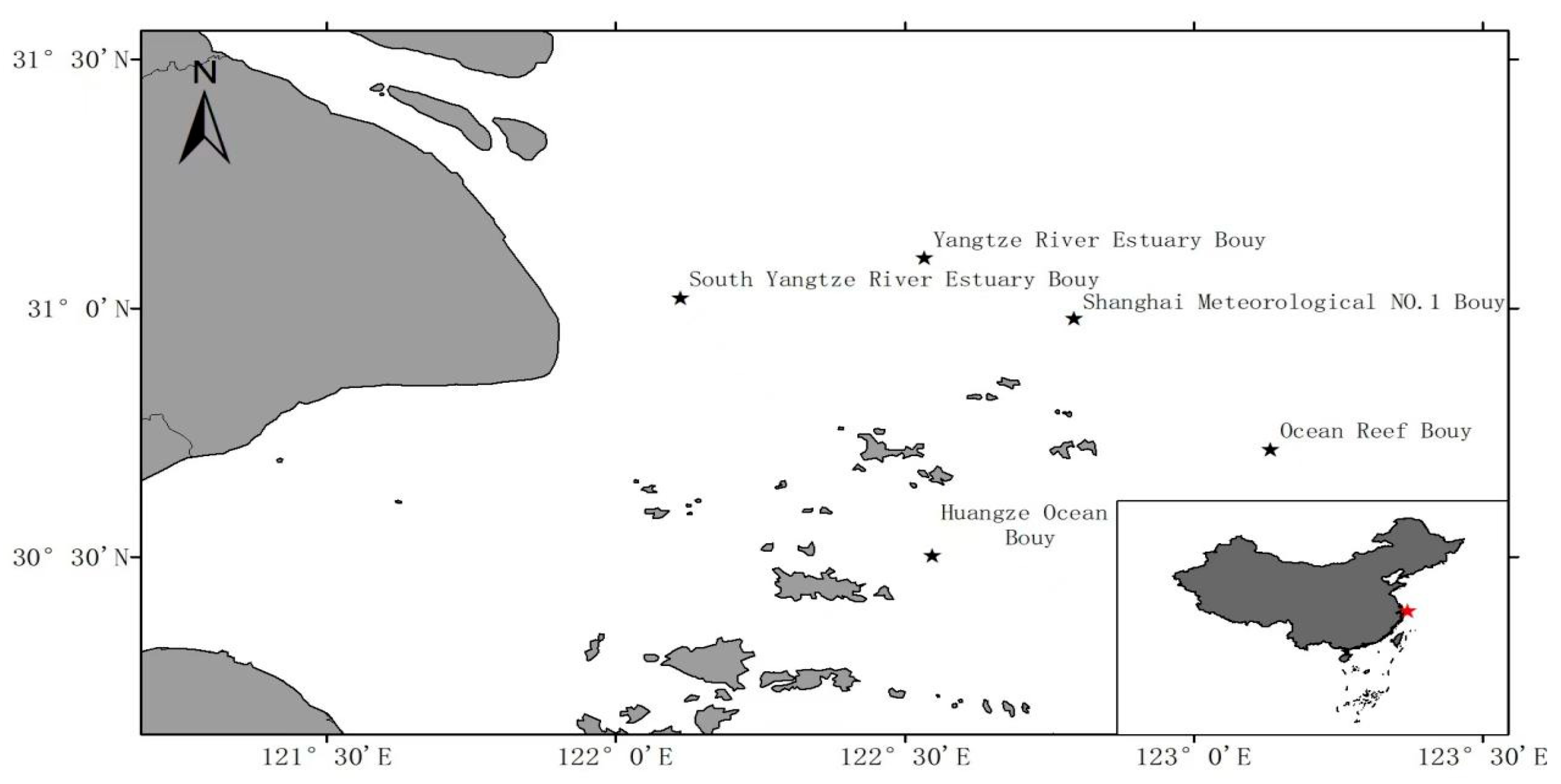
Figure 1. The geographical distribution of buoy stations (black and red stars indicate locations of the buoy stations and the Yangtze River Estuary of China respectively).
Atmosphere 14 00682 g001
Figure 2. Wavelet analysis of daily 10-m wind speed at the Yangtze estuary in winter half-years (from November to April of next year) of 2011–2017. (Shaded areas denoting above the confidence level of 90%, and dashed lines indicating the boundary effect).
Atmosphere 14 00682 g002
Figure 3. Significant period (median value shown) of low-frequency oscillations of 10-m wind speed corresponding to SGPs in the Yangtze River Estuary (unit: day). (Black dots denoting SGPs).
Atmosphere 14 00682 g003
Figure 4. Wind speed anomaly and 10~30 day LFO components at 8 phases of the 10~30 day low-frequency oscillations of wind speed associated with SGPs.
Atmosphere 14 00682 g004
Figure 5. 500 hPa geopotential height anomaly field at phase 1 (a); phase 3 (b); phase 5 (c); and phase 7 (d) of the 10~30 day low-frequency oscillations of the 10-m wind speed associated with SGPs (unit: gpm).
Atmosphere 14 00682 g005
Figure 6. 500 hPa geopotential height anomaly field at phase 1 (a); phase 3 (b); phase 5 (c); and phase 7 (d) of the 10~30 day low-frequency oscillation of wind speed associated with SGPs (unit: gpm).
Atmosphere 14 00682 g006
Figure 7. 200 hPa wave activity flux (vectors) at phase 1 (a); phase 3 (b); phase 5 (c); and phase 7 (d) of the 10~30 day low-frequency oscillation of wind speeds associated with SGPs (Contours indicate the disturbance flow function and arrows indicate wave activity flux).
Atmosphere 14 00682 g007
Figure 8. Schematic diagram of the key regions of SGPI construction. (Red boxes with “1” and “2” denoting the key regions of SGPI.).
Atmosphere 14 00682 g008
Figure 9. Sub-seasonal forecast verification of SGP hindcast and forecast in winter half-years of 2011–2021.
Atmosphere 14 00682 g009
Figure 10. The scatted diagram (red dots) of the sub-seasonal hindcast/forecast scores of SGPs in Figure 9 and SGPI strength during the 30 days before the initial forecast time (The black line indicating the linear fitting line, the numbers next to the red dots representing the hindcast/forecast year).
Atmosphere 14 00682 g010
Disclaimer/Publisher’s Note: The statements, opinions and data contained in all publications are solely those of the individual author(s) and contributor(s) and not of MDPI and/or the editor(s). MDPI and/or the editor(s) disclaim responsibility for any injury to people or property resulting from any ideas, methods, instructions or products referred to in the content.