Abstract
The Royal Belgian Institute of Natural Sciences launched its airborne sniffer program in 2015 whereby a custom-built sniffer sensor was installed onboard the Belgian coastguard aircraft enabling the measurement of SO2 and NOx emitted by ocean-going vessels (OGVs). The data gathered on non-compliant OGVs were subsequently sent to port inspection authorities, who were then able to trigger inspections more rapidly than had they not had the data from the aircraft. This study reveals the added value of airborne alerts on port inspection effectiveness, a subject that had not been previously documented. This article demonstrates that airborne alerts have not only led to increased sanctions but have also drastically improved the efficiency of port inspection authorities, leading to a 50% reduction in the enforcement cost per confirmed violation. Port inspection authorities were able to follow up on 46% of the generated Fuel Sulphur Content (FSC) alerts. Of the alerts that were followed up, 43% were confirmed as non-compliant after inspection. This means that 20% of the total number of generated airborne alerts, which includes those that were not able to be followed up, met conditions for legal sanctioning. In contrast, for NOx alerts, only limited follow-ups were conducted by port inspection authorities. None of the alerts were confirmed with those inspections, mainly due to the lack of inspection mechanisms for real-world NOx emissions under IMO and EU regulations. In addition, for this study, a large-scale remote FSC measurement validation analysis was conducted for the first time, comparing airborne FSC measurements and FSC reference data. In order to obtain FSC reference data, onboard measurements from exhaust gas cleaning systems (EGCSs) were collected, together with fuel samples from Belgian port inspection authorities. The validation analysis revealed that the empiric deviation in the airborne FSC measurements with the FSC reference data was 9%, which was significantly lower than the 25% uncertainty used in the reporting of the alerts. This study helps pave the way for an increased role of airborne monitoring in the MARPOL Annex VI enforcement chain.
1. Introduction
1.1. Background to MARPOL Annex VI
The SOx and NOx emission limits from ocean-going vessels (OGVs) are laid down by the International Maritime Organization (IMO) in the MARPOL Protocol of 1997 (MARPOL PROT 1997, as amended), described in the MARPOL Annex VI. Reference to Annex VI in this article will be to the Revised MARPOL Annex VI in 2008 and not to the 2021 Revised MARPOL Annex VI because airborne emission measurements took place before entry into force of the 2021 revision [1]. In MARPOL Annex VI, designated emission control areas (ECAs) were defined with more stringent standards for SOx and NOx.
MARPOL Annex VI Regulation 14 defines the SOx emission limits. As of 2008, the Baltic Sea and the North Sea were designated as sulfur emission control areas (SECAs) (Figure S1, upper). The maximum fuel sulfur content (FSC) of the marine fuels used by OGVs in SECAs was reduced in successive steps until it reached the current limit of 0.1% FSC. Instead of using compliant fuels, OGVs can also use natural gas or an exhaust gas cleaning system (EGCS) to achieve the same emission level as low-sulfur fuels (Table S1) [2,3,4,5]. The sulfur limit outside SECAs, initially set in 2005 to 3.5% [1,4,6], was reduced in 2020 to 0.5% by the so-called ‘Global Sulfur Cap’ [7] (Figure S1, middle). On 1 March 2020, the so-called “Carriage Ban” came into force, prohibiting the carriage of non-compliant fuels in the bunker tanks, unless the OGV is equipped with an EGCS [8].
Moreover, at the European level, SOx emissions from OGVs are regulated by the EU Sulphur Directive ((EU) 2016/802) and the Commission Implementing Decision ((EU) 2015/253), which lay down the rules regarding sampling and reporting of the sulfur content of marine fuels [9,10,11,12]. The latter stipulated that Member States must carry out documentary inspections on at least 10% of the total number of individual OGVs calling at Member States’ ports (Art 3.1, Implementing Decision). In addition, 40% of the inspected ships will be checked using approved (laboratory) fuel sampling methods for Member States that fully border the SECA area (Art 3.2(a)). However, the number of fuel samplings can be reduced by up to 50%, by subtracting the number of OGVs that have been checked for compliance using remote sensing or the rapid scan analysis (Art 3.3(a)) [11]. At the national level, Belgium further implemented MARPOL Annex VI and the Sulfur Directive ((EU) 2016/802) in 2020 [13].
MARPOL Annex VI Regulation 13 introduced NOx emission limits for OGVs and described dedicated NOx emission control areas (NECAs) where stricter limits apply for recently built OGVs (Tier III, see further in this section) [5]. Five years after the enactment of the North American and US Caribbean NECA on 1 January 2016 [14], the SECA in the Baltic Sea and the North Sea was expanded in 2021 with a NECA and renamed emission control area (ECA) [15,16]. To reduce NOx emissions in the OGV exhaust gases, engine manufacturers have the option to either tackle the combustion processes in the engine or to install NOx abatement systems such as a selective catalytic reduction (SCR) and/or exhaust gas recirculation (EGR) [17].
MARPOL Annex VI divides the merchant fleet into four categories, from tier I to tier III, and before tier I (tier 0), according to the construction of the ship based on the keel-laying date (KLD) or a similar stage of construction (Reg. 2.19). The emission limits per tier follow a decreasing curve in the function of the engine-rated speed (ERS or n), expressed in rotations per minute (RPM) (Figure S1, lower). In order to obtain the required Engine International Air Pollution Prevention (EIAPP) Certificate, a verification test is executed before the installation of the engines onboard the OGV, in accordance with the NOx Technical Code, MEPC.1/Circ.679 [18,19]. After the installation of the engines onboard, an International Air Pollution Prevention (IAPP) Certificate is issued by a classification society. In addition, the NOx Technical Code stipulates that all interchangeable parts that exert an influence on the NOx emissions, described as “engine components” (1.3.3, NOx Technical Code), must be listed in the NOx technical file and all modifications must be recorded and stored onboard together with the EIAPP Certificate and the IAPP Certificate [18,20]. Substantial modifications mean all modifications to the engine components that may cause NOx emissions to exceed the limit, in which case a new verification test is required (6.4.16.1, NOx Technical Code). In contrast, the replacement of engine components that do not alter the NOx emissions are not considered a substantial modification (1.3.2 NOx Technical Code). The verification tests are based on five different engine test cycles with four to five engine loads and corresponding weighting factors (WFs) (Table S2). It is crucial to highlight that only for Tier III, a “not to exceed” (NTE) limit is defined, which states that the NOx emission may not exceed the limit by more than 50% at any of the individual engine loads [18]. Another critical aspect of the Technical Code to highlight is that currently, no restrictions are described under the 25% main engine loading point for any of the tiers.
In contrast to the sulfur regulations, NOx emissions from ships are currently not regulated by an EU directive. However, discussions are ongoing to evaluate if MARPOL and its Annexes, thus including NOx emissions, can be included under a future revision of the Ship Source Pollution Directive (2005/35/EC) [21]. More importantly, on 18 December 2022, the European Commission, the European Parliament, and the Council of the EU finalized a Provisional Agreement on a broad set of policy proposals for the “Fit for 55” climate package, including a landmark reform of the EU Emissions Trading System (ETS) and the milestone introduction of the Carbon Border Adjustment Mechanism (CBAM), which still requires formal approval from the Parliament and the Council before entering into force. Particularly, once formally adopted, the new ETS system will, for the first time, integrate emissions from the maritime sector into its scope, with the obligation to surrender allowances rising from 40% of verified emissions in 2024 to 100% in 2026. Moreover, in addition to the gradual implementation of CO2 emission retributions, OGVs will also have to pay for their non-CO2 emissions, such as N2O and CH4, from 2027 [22,23,24]. At the end of 2024, it will be decided if other greenhouse gasses, such as NOx, and certain particles, such as Black Carbon (BC), will be included in the ETS [25,26,27].
1.2. Research Questions
In order to create an adequate compliance level for the MARPOL Annex VI Regulation 13 and 14, an effective enforcement strategy is required that incorporates a reasonable non-compliance detection rate. The legal sanctions need to be in proportion to the economic benefit that would result from an OGV being non-compliant to discourage violations. Such an effective enforcement strategy will not only contribute to environmental protection, human health, and economic benefits but will also contribute to a level playing field for the maritime transport sector [28,29,30,31,32]. Therefore, ensuring that all market actors follow the same set of rules and conditions is considered one of the backbones of international trade [33,34,35,36].
Remote measurements from either fixed stations or airborne platforms have been shown to provide an efficient solution to monitor the compliance of OGVs with regard to the emission regulations and, therefore, have the potential to contribute to the enforcement strategy and level playing field [37,38,39,40,41,42,43,44,45,46,47,48,49,50,51,52,53,54,55,56,57,58,59,60]. Even so, the use of airborne measurement data has not yet been recognized as independent legal evidence for observed possible non-compliant OGVs and is thus far merely used for risk-based targeting of inspections in ports. However, the impact of the provision in these airborne alerts on the effective results of port inspections of OGVs has not been examined in detail to date. The main research question of this study was to evaluate how and to which extent airborne measurement alerts have already contributed to the efficiency and results of inspections in Belgian and North Sea ECA ports. Looking ahead, this study also examines the full potential role of airborne monitoring for the targeting of inspections.
In addition, to increase the enforcing effect of airborne monitoring, the airborne measurements would need to obtain a legal evidence status, not only to serve as an alerting mechanism but also to become a direct enforcement action. An essential part of the process for receiving the status of legal recognition of airborne measurements is the validation of airborne measurement reliability in real-world conditions. So far, several studies have been executed comparing onboard measurements with remote measurements. However, these studies were limited to one or two OGVs and concerned only one OGV type [37,38,53,61,62,63,64]. The third research question of this study was therefore to evaluate how airborne measurements would relate to real-world emissions for a larger amount and more diverse sample of OGVs.
Finally, airborne operations and airborne measurements, in particular, are known to be costly endeavors. Previous studies have already demonstrated the advantage of scale in airborne measurements [31,42,43]. The third research question focuses on evaluating the overall cost-effectiveness of airborne operations compared to other remote measurement methods and onboard inspections.
2. Methods and Materials
2.1. Airborne Measurements
The Scientific Service of the Management Unit of the Mathematical Models of the North Sea (MUMM) of the Royal Belgian Institute of Natural Sciences (RBINS) is recognized by Belgian Law as one of the legally competent authorities for the monitoring and enforcement of MARPOL regulations at sea [65]. Since 1991, MUMM has been responsible for airborne surveillance of the Belgian North Sea area and neighboring waters in the so-called Bonn Agreement (BA) Quadripartite Zone of Joint Responsibility (BAQPZJR) (Figure S1, upper).
Since 2015, the RBINS has been conducting airborne surveillance operations to monitor sulfur emissions from OGVs in accordance with MARPOL Annex VI Regulation 14 [39]. In addition, from 2020 onwards, the RBINS has been conducting airborne surveillance operations to monitor NOx emissions from OGVs in accordance with MARPOL Annex VI Regulation 13 [39,40,41].
Based on the measurement uncertainty, thresholds were described that reflect not only the uncertainty level but also the level of non-compliance. Three flags of color were defined for both SO2 and NOx. For the lowest alert level, the yellow flag with a confidence interval (CI) of 68% (σ = 1) was used. For the orange flag, a CI of 95% was used (σ = 1.96); for the most excessive pollution alerts, a red color flag was defined based on the 99% CI (σ = 2.576) (Table 1). The uncertainties align with the results of other organizations and previous measurement campaigns using similar techniques [38,42,46,47,48,54].

Table 1.
Applied thresholds for FSC and NOx compliance monitoring.
Once a possible violation was observed, a flight report was sent to the port inspection authorities. In addition, the alert was shared in the Thetis-EU database and became accessible to all EU Member States (Section 2.3) [39,40,46]. The provision of airborne alerts may therefore be considered the first step in the enforcement chain. The onboard inspection executed by the port inspection authorities is the second step in the enforcement chain (Figure 1).
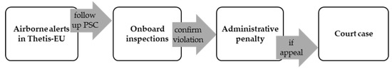
Figure 1.
Flow chart illustrating the 4 steps of the MARPOL Annex VI enforcement chain.
2.2. Port Inspections
The various international emission regulations for OGVs are mainly enforced by onboard inspections in ports. In general, this is done under the jurisdiction of port state control (PSC). In Belgium, inspections regarding the sulfur regulations are the responsibility of a separate service called ‘Environmental Safeguarding and Dangerous Goods’ within the department ‘Shipping Control’ of the Federal Public Service (FPS) Mobility and Transport. This separate service has eight environmental inspectors, which operate next to PSC and control compliance with the EU Sulfur Directive (EU) 2016/802. Not being part of PSC means that those inspectors cannot arrest vessels, but in the case of breaches in the sulfur regulations, they make police reports based on documentation requirements and fuel controls. These inspectors have no access to the Paris MoU Thetis database (PSC) but only to the Thetis-EU database (Section 2.3).
Inspections are executed in accordance with the IMO and EU guidelines, whereas fuel samples are collected from a location in the fuel supply lines as close to the main engine as possible. This location is always decided in close cooperation with the chief engineer and is most often either from a dedicated sampling point or close to the last booster filter. A fuel sample is collected in one sampling bottle (1 L), and after mixing, is dispersed over two other bottles; one bottle remains onboard to be used as counter-expertise if necessary. The other two bottles are taken along by the inspector, one of them is sent to an accredited laboratory for analysis using an X-ray fluorescence (XRF) spectrometer (accuracy of 0.01% FSC), and the other sample is stored and kept as a reference sample in case a violation was observed in the first sample [11,66].
In the case that an onboard inspection demonstrates non-compliance with an FSC above 0.15% FSC, the environmental inspectors shall make a police report. On the basis of this report, the administrative sanctioning department of FPS Mobility can impose an administrative fine. This sanctioning step can be considered the third step in the enforcement chain. If the accused party does not agree with the proposed administrative fine, this party can appeal using a suspending petition before the Court of First Instance, which can be considered as the fourth and final step in the enforcement chain, without a possibility of appeal (Art. 16, Law of 25/12/2016) [67] (Figure 1).
2.3. Thetis-EU
A dedicated webtool, called Thetis-EU, was created by the European Maritime Safety Agency (EMSA) to record information on the results of individual compliance verifications carried out by Member States’ competent authorities under the Sulphur Directive (EU) 2016/802. Thetis-EU also serves as a platform to exchange information on remote measurements from and between EU Member States. Thetis-EU should not be confused with Thetis, which is the ship inspection database of the Paris MoU. Thetis-EU was established following the Commission’s Implementation Decision, which stipulates that a system for the reporting of inspection results is mandatory. However, Member States have the discretionary power to choose whichever reporting system they prefer, and the use of Thetis-EU is therefore on a voluntary basis [11,12,68]. The inspection results and alerts in Thetis-EU are accessible to all EU Member States and two EEA EFTA States—Iceland and Norway. Data on inspections and compliance levels can be publicly accessed [68]. For detailed inspection results of specific OGVs, authorization has to be granted by the Thetis-EU National Competent Authority (NCA). For Belgium, this NCA lies with the FPS Mobility and Transport, and a request for read-only access is granted to the crewmembers of the coastguard aircraft.
When an OGV with an alert enters a port in another EU Member State, local port inspection authorities can see this alert and start an inspection. Therefore, Thetis-EU facilitates the link between step one and step two of the enforcement chain (Figure 1). It is noteworthy that the local authorities do not receive an active warning from Thetis-EU when an alerted OGV is heading to their jurisdiction. Instead, authorities have to check manually if alerted ships are calling at their ports. Consequently, there is no prioritization system for inspections as is the case with the Thetis system under the Paris MoU on PSC.
For optimizing the reporting to Thetis-EU and improving the efficiency of port inspections, in 2019, RBINS implemented an automatic upload of the airborne measurements to Thetis-EU. By doing so, Belgium was the first Member State to upload monitoring data directly into Thetis-EU. In addition to non-compliant alerts, these data also include compliant data. This compliant information is highly valuable for port inspectors as it allows a more efficient targeting of the inspections by ignoring OGVs that were recently found to be compliant.
2.4. FSC Data Validation with Reference Data
A validation analysis has been carried out to compare the airborne measurements with real-world reference FSC data. Two types of data were used for the collection of reference FSC data. For the first type, FSC information was collected from fuel samples. For the second type, SO2/CO2 ratios were collected from vessels equipped with an EGCS.
2.4.1. FSC Comparison with Fuel Samples
For the large majority of the airborne alerts, data were submitted to Thetis-EU. In the case that an onboard inspection was carried out in the next port of call, the fuel sampling results were entered in Thetis-EU by the port inspection administration. The results of those fuel sample analyses have been retrieved for warnings generated by the aircraft. As the alerts concerned mainly non-compliant data, this can create a bias in the data comparison. Therefore, additional fuel samples were taken by the Belgian environmental inspectors for airborne measurements of compliant OGVs.
2.4.2. EGCS Data
OGVs that are equipped with an EGCS are required to have a continuous emission measurement system (CEMS) that logs specific emission-related data (7, Data recording) [2]. This system is a vital part of the proper functioning of the EGCS, which is used to provide SO2 removal rate feedback to the EGCS control unit. This feedback is essential to ensure, on the one hand, that the emissions are never over the limits defined by IMO [2]. On the other hand, this also allows the OGV to optimize the EGCS capacity to avoid over-scrubbing, which would cause higher fuel consumption and discharge water with lower PH levels. Discharges of wastewater with low PH levels are not only corrosive for the piping but moreover, may also not be in accordance with the regulations. The IMO guidelines for EGCS stipulate that the minimum PH of the discharge wastewater is 6.5 or no less than 2 PH levels different from the inlet water (10.1.2) [2]. The CEMS data are logged according to the IMO guidelines for EGCS [2] and can be requested for verification by port inspection authorities. CEMS data include measurements of SO2 (in ppm) and CO2 (%Vol), which are used to calculate the SO2/CO2 ratio (1.3). In accordance with the 2015 IMO guidelines for EGCS, this ratio must be below 4.3 in the SECA (1.3) (Table S1) [2], which corresponds to an identical conversion used by the sniffer software (with the difference in the units). This procedure is described in Appendix II of Resolution MEPC. 259 (68) [2].
The data from the EGCS logs, therefore, provided an excellent set of reference data to validate the airborne measurement data. For this purpose, seven shipping companies were contacted to request if CEMS data from their OGVs could be provided for the times when they were measured with the aircraft. The shipping companies were selected based on the number of airborne measurements and OGV type (container, RoRos, tanker, and bulk carriers). Four companies agreed to cooperate and provided CEMS information for the period 2018–2022. Unfortunately, no tanker and no container OGVs were among the participating companies, as one of the companies requested to remain anonymous, and no information was shared with the other participating companies.
Although the IMO guidelines recommend that UTC time be used for the data logging (Art 7.2) [2,69], often a time correction had to be applied as it was observed that for some OGVs, the time and location of the log files did not match with the coordinates from the Automatic Identification System (AIS) of the OGV at the moment of the measurements. To correct for any short-term differences, an average SO2/CO2 ratio has been applied for the two CEMS measurements before and the two CEMS measurements after the moment of the airborne measurement. Some OGVs were equipped with multiple EGCSs, for which the average values of the different EGCSs were calculated. Most of the voluntarily provided information concerned compliant data. However, some non-compliant measurements were also included for which CEMS log data was obtained after a port inspection, including from container OGVs. As a consequence, only tanker OGVs were missing in the final dataset.
2.5. Statistical Analysis
A Kolmogorov–Smirnov test was used to assess the normality of the emission measurement data. With a p < 0.05, the data were considered not normally distributed. Therefore, non-parametrical tests were used. A two-tailed Kolmogorov–Smirnov test was used to compare the distribution in the measurements of different sources (i.e., ship inspection data versus airborne data). Distributions were discovered to be significantly different when p < 0.05 [70]. To determine a difference in the compliance rate between two distributions, a two-sided chi-square test was used. Statistical significance was defined when p < 0.05 [71,72]. When Type I errors are used, they refer to the number of false positives; when Type II errors are used, they refer to the number of false negatives [70].
To compare the correlation between (n) reference FSC (FSCref) and airborne measurements (FSCAC), a Pearson correlation coefficient (r) was used in addition to a modified Bland Altman (B&A) visualization. A B&A visualization is commonly used for the comparison of two measurement methods and provides an alternative for a correlation or linear regression with a corresponding coefficient of determination (R2). The main advantage is that it provides a quantification of the agreement between two methods based on the determination of Limits of Agreement (LOA) that can be evaluated according to a user predefined Maximum Allowable Difference (MAD). The B&A visualization furthermore allows for the evaluation of the absolute and proportional bias [73,74]. For a B&A visualization, the difference between the results of the two measurement methods is plotted against their average. The LOA are generally defined by the ±Standard Deviation (SD) (±LOA). For the LOA with the Confidence Interval (±LOA + CI), the SD is multiplied by the sigma value (σ) for which generally 1.96 is used. If the ±LOA and/or the ±LOA + CI are within the ±MAD, both measurement methods can be considered comparable.
For the modified B&A visualization in this study, the difference between the reference measurements and the airborne measurements was plotted against the average FSC. The standard B&A was modified for the use of the SD in combination with the Relative Standard Deviation (RSD). To create the MAD, the sulfur limit (S) was used as defined within the thresholds, for yellow flags (0.13–0.2% FSC), S is 0.1% FSC; for orange flags (0.2–0.3% FSC), S = 0.11% FSC; for red flags (>0.3% FSC), S is 0.15% FSC. The MAD was defined to ensure that the difference between the airborne measurement and the reference data is never more than S, avoiding, therefore, Type I errors.
3. Results and Discussion
3.1. Follow-Up on Airborne FSC Alerts by Port Inspection Authorities
3.1.1. Results of Onboard Inspections
For Belgium, it was defined, in accordance with the EMSA, that ca. 5500 OGVs are calling Belgian ports every year. According to the Commission Implementing Decision ((EU) 2015/253), inspections must be carried out on 10% of these port calls (Art 3.1), which amounts to 550 inspections per year. Belgian inspection authorities started with sulfur inspections in 2015, but as they only carried out five inspections in that year, 2016 is used as the starting point. In total, 12,148 onboard inspections were completed between 2016 and 2022 (Figure 2A). With an average of 1735 inspections per year, this is substantially higher than the 550 mandatory inspections. The Commission’s Implementation Decision further indicates a 40% fuel sampling effort for MS bordering a SECA (Art 3.2.), representing 220 fuel samples. However, a reduction of up to 50% may be applied when remote monitoring is used (Art 3.3), which comes down to 110 mandatory fuel samples per year [11]. In total, 871 fuel samples were taken between 2016 and 2022, or 124 fuel samples per year on average, therefore amply fulfilling the required number of fuel samples.
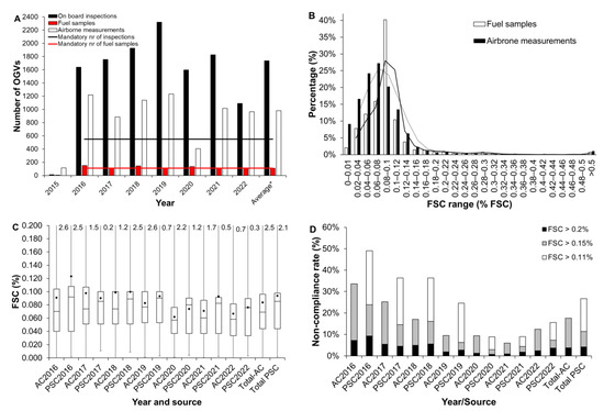
Figure 2.
Overview of the number of mandatory and executed onboard inspections (black) and fuel samples (red) undertaken by Belgian port inspection authorities and airborne measurements (white) (A). Comparisons of observed FSC values and moving averages of fuel samples with airborne measurements between 2016 and 2022 (B). Boxplot comparison of FSC between fuel samples and airborne measurements with 25, 75% percentile, median values, and average values (♦) (C). Comparison of compliance rates between port inspections and airborne monitoring between 2016 and 2022 (D).
During the global COVID-19 pandemic, the number of port calls in Belgian ports decreased by 8% in 2020 and by 5% in 2021 compared to 2019 [75]. Despite this, Belgium still managed to meet the pre-COVID set number of inspections and fuel samples, which contrasts with the impact of the pandemic within the Paris MoU, for which a 27% reduction in the number of PSC inspections was reported [76].
When in port, the overall FSC non-compliance is assessed based on the document inspections, and the compliance rate is very high; 99.5% of the OGVs had an FSC under 0.15%. When looking at the compliance rate based on fuel samples alone, compliance is substantially lower, with 92.2% of the OGVs under 0.15% FSC. The average FSC from the collected fuel samples was 0.096% FSC.
3.1.2. Results of Onboard Inspections
Regarding airborne monitoring, between 2016 and 2022, 6961 OGVs were checked for FSC, with an average of 978 OGVs per year. A total of 626.5 flight hours were spent on MARPOL Annex VI surveillance or an average of 89.5 flight hours per year, and of the measured OGVs, 93.6% were considered compliant, and the mean observed FSC was 0.084% FSC.
The Belgian average FSC and non-compliance levels are slightly higher when compared to other studies and measurement campaigns [42,51,52,54,77,78,79,80,81,82,83,84,85]. This is most likely related to (1) the closer distance to the SECA border, leading to a higher likelihood of observing OGVs who either delayed (outgoing traffic) or advanced (ingoing traffic) their fuel change-over procedures; (2) the closer proximity of the Belgian coastguard aircraft to the OGVs during the measurement, resulting in higher gas concentration peaks; and (3) the use of special plume simulation mixtures during the calibration, eliminating the measurement bias [39,40,86,87]. When looking at other NOx studies, similar NOx emission factors have been observed. Like the Belgian results, other studies have also indicated lower non-compliance levels for NOx compared to FSC. The most important finding, indicating higher non-compliance levels for Tier II and Tier III compared to Tier I, has also been confirmed in other studies [50,85,88,89,90,91,92,93].
Some authors have elaborated that environmental factors such as temperature (T) and relative humidity (RH) may influence the remote measurements of FSC [42,44,54]. In addition, both T and RH are known to have an impact on NOx emissions and are therefore included as a correction factor in the NOx Technical code [17,18,41,94]. For this reason, the seasonal and environmental effects on the airborne measurements were analyzed using an evaluation of the monthly average, median, and non-compliance levels. For the calculation of these monthly values, a total of 100 measurements were set as the minimum per month. For FSC, the months of March–November provided sufficient data, whereas for NOx, the months of March–October were used. The monthly averages, median, and non-compliance levels for FSC showed very little variation, with an SD of 0.01% FSC for both the average and median FSC and an SD of 1.8% for the FSC non-compliance level. For the monthly average and median NOx, an SD of 0.6 g NOx/kWh was found, and the SD of the NOx non-compliance was 1.4%. The visualization of the average, median, and non-compliance FSC showed higher levels in the summer compared to the winter (Figure S4A). However, the effect is weak, with a large variation in non-compliance between the summer months. For NOx, no seasonal relation could be observed (Figure S4B).
To evaluate the impact of the T and RH on the FSC and NOx measurements, the monthly average T and RH were normalized and plotted together with the normalized median and non-compliance rate for FSC and NOx [95]. This showed hardly any impact of the T and RH on the median FSC; however, a limited T effect on the FSC non-compliance rate was observed, and this effect corresponds with the observed seasonal effect (Figure S4C). The T and RH did not have any impact on either the median NOx or the NOx non-compliance rate (Figure S4D). In addition, the R2 values for the linear regression between these monthly FSC and NOx values and the monthly average T and RH were calculated to evaluate the impact of environmental factors on the airborne measurements (Table S3). This showed low to very low R2 values, with 0.3–0.4 for the median and average FSC and 0.02–0.2 for the median and average NOx. A higher but still low R2 of 0.6 was found for the non-compliance of FSC with T, confirming the seasonal effect. On the other hand, the R2 for the FSC non-compliance with RH was 0.00. The R2 was also 0.00 for the linear regression between the NOx non-compliance and T, as well as for the RH.
Due to the limited or lack of seasonal and environmental effects on the airborne measurements, their impact was not taken into account during the further data analysis in this study. This does not imply that there are no environmental or seasonal effects to be considered for the remote measurement of FSC and NOx. Merely, it can be stated that these factors had no significant impact on the remote measurement data in this study. This could be due to the relatively high measurement uncertainty and/or the limited seasonal variation over the Belgian waters from spring until fall.
3.1.3. Comparison of Port Inspection and Airborne Results
The significant difference in the number of fuel inspections between port inspections and airborne inspections immediately demonstrates the scale advantage of airborne monitoring. It takes 275-man hours per year to carry out 110 fuel samples in the port (only including the time of the inspection), while for 110 measurements, 10 flight hours would suffice, with a crew of four on board or 40-man hours, so almost 7 times more time efficiency.
When comparing the FSC measurement distribution between the aircraft and fuel inspections, they broadly show the same patterns. The aircraft measurements have the highest proportion in the 0.06–0.08% FSC interval (median = 0.086% FSC), and the fuel samples have a higher proportion in the 0.08–0.1% FSC interval (median = 0.069% FSC) (Figure 2B). This difference is also observed in the average FSC values, which indicates that the average FSC of the airborne measurements is 0.084% FSC, significantly lower than the average measured FSC in the port of 0.094% FSC (p < 0.001) (Figure 2C). To exclude the effect of the airborne alerts, the average FSC was calculated for the fuel samples excluding the samples carried out after airborne alerts, which was 0.087% FSC. Although the difference was lreadyy much smaller, it still appeared to deviate significantly from the average FSC from airborne measurements (p < 0.001) (Figure S2, upper), which indicates the presence of a slight negative measurement bias for the airborne measurements. This average FSC for the fuel inspections without alerts was furthermore compared with the average FSC for the fuel inspections that followed up on an alert, which was with 0.21% FSC significantly higher (p < 0.001) and even exceeding the 0.1% FSC legal limit substantially (Figure S2, lower), therefore demonstrating the added value of the airborne surveillance.
It is not easy to draw conclusions about the compliance rates between the airborne results and the results of either the onboard inspections or the fuel samples (Figure 2D). Onboard inspections may miss non-compliance if no suspicious aspects in the documents are observed (Type II errors). Fuel samples, on the other hand, may be biased as they are not taken randomly but are taken after suspicious aspects in the documents, after an alert from airborne monitoring, or due to previous deficiencies. When the overall compliance based on the document inspections is compared to the airborne compliance rate, the airborne compliance rate is significantly lower (p = 0.000). When the compliance rate based on the fuel samples is compared to the airborne results, the airborne compliance is significantly higher (p = 0.0281).
However, to compare the compliance rate of the airborne measurements with the unbiased fuel sampling, the number of fuel samples greater than 0.15% FSC, excluding the fuel samples initiated after the airborne alert was calculated as 94.1%. The number of airborne measurements exceeding 0.15% FSC was 94.2%, which is highly comparable. In general, the difference was not found to be significant (p = 0.8691).
3.1.4. Follow-Up on Alerts Based on Thetis-EU
All possible non-compliant OGVs observed with the coastguard aircraft were reported to the Belgian port inspection authorities by email. Only about 1/3 of the observed potentially non-compliant OGVs went to a Belgian port. In the case that the non-compliant OGVs were sailing to a Belgian port, inspectors of FPS Mobility prioritized these OGVs for inspection and carried out an inspection on board whenever it was operationally feasible. In case the non-compliant OGV was not sailing to a Belgian port, an alert was made in Thetis-EU. Initially, this was completed manually using FPS Mobility, but from 2019 onward, the results were automatically uploaded to Thetis-EU after each flight. Once an OGV was inspected in a Belgian or another EU port, inspectors reported this in Thetis-EU. For all airborne alerts, a manual check was carried out to see whether actions had been taken, as Thetis-EU does not (yet) contain a tool that can generate those exports. For the evaluation of the follow-up, a qualitative approach was used to see if the OGV was followed up within a reasonable time. For OGVs operating only in the ECA, a limit of 14 days was used; for OGVs operating on international routes, it was checked if the OGV was inspected upon their return to the ECA (within a maximum of 3 months).
In terms of analyzing the follow-up on airborne alerts by port inspection authorities, a distinction was made between Belgian and other EU ports of destination (Figure 3A). In 2015, only five inspections were carried out in Belgium. Moreover, the airborne measurement was taken in a test period without the results put into Thetis-EU, and thus 2015 is omitted from the analysis. In 2016, only 34 of 120 alerts were followed up (28%). This low follow-up was mainly due to the limited follow-up on alerts in Thetis-EU, as 24 alerts out of 46 alerts for Belgian ports were followed up, and only 10 out of 74 alerts for other EU ports were followed up. In 2017, the overall follow-up improved to 59%, with 16 out of 18 alerts followed up in Belgian ports and 13 out of 31 alerts in other EU ports. In 2018, the overall follow-up increased further to 60%. Again, the follow-up in Belgium was very high with 19 out of 21 alerts. In addition, the follow-up in other EU ports increased with 25 out of 52 alerts followed-up. In 2019, there were fewer alerts reported, resulting in a limited decrease in the follow-up to 55%, with 12 out of 19 alerts in Belgium, and 16 out of 32 alerts in other EU ports. In 2020, due to the global COVID-19 pandemic, the global follow-up fell substantially back to 38%: one alert was delivered to Belgian ports, which was followed up, and two out of seven alerts were followed up by other EU ports. In 2021, the overall follow-up increased again to 59%, three out of four alerts in Belgian ports were followed up, and in other EU ports, 7 out of 13 alerts were followed up. In 2022, more alerts were generated, whereas the follow-up fell back to 49%, with 8 out of 13 alerts followed up in Belgian ports and 15 out of 34 in other EU ports. During 2016–2022, 83 out of 122 reported FSC alerts to a Belgian port were followed up (68%), and 88 out of 243 alerts were followed up in other EU ports (36%) (Figure 3A). The overall follow-up of airborne alerts for OGVs with all ports of destinations combined is 46%, which can still be considered relatively high, as 20% of the observed OGVs had a port of destination outside the SECA.
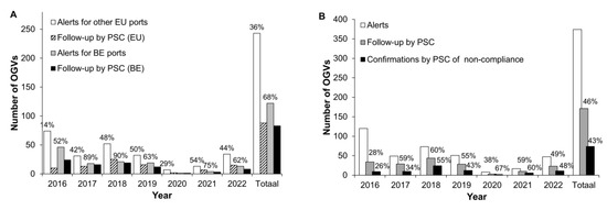
Figure 3.
Follow-up of alerts for OGVs in Belgian ports and follow-up of alerts for OGVs in other EU ports (A). Number of alerts send to port inspection authorities, number of alerts followed-up, and number of confirmations (B). Alerts for EGCS OGVs (% of the total number of alerts), number of alerts followed-up with port inspection, and number of EGCS OGVs confirmed after inspection (C). Improvement in the efficiency of PSC inspections (D).
3.1.5. Confirmation Rate of Airborne Alerts in Ports
The confirmation of the airborne alerts was analyzed based on the results of the fuel sampling, entered in Thetis-EU after an alert was followed up by port inspection authorities. An alert was considered to be confirmed as soon as the measurement of the fuel sampling was above 0.11% FSC. In Belgium, a public statement and financial penalty are only applied above 0.15% FSC, and this limit was investigated separately.
In the period 2016–2022, port inspection authorities in Belgium and in other EU countries were able to confirm the alert in 43% of the cases, after an inspection had been carried out onboard the OGV (Figure 3B). Noteworthy is that the confirmation rate is lower for Belgian ports (39%) compared to other ports (48%), which is likely due to the fact that most alerts for OGVs with a Belgian port of destination went to Antwerp (22% of the observed OGVs), while OGVs with another country as a destination went to Rotterdam (17% of the observed OGVs) (Figure S3). OGVs going to Antwerp must sail on the river Scheldt, which takes 5–6 h, adding several hours to the time lap between the measurement and the fuel sampling, hence decreasing the chance of confirming the non-compliance.
The reason why the port inspection authorities did not always confirm the initial alerts may be due to several factors. One of the factors is time: on average, the time between the alert and the onboard inspection was 49 days. In the meantime, the OGV might have completed the fuel changeover procedures or switched to compliant fuel. The median time to successfully confirm the non-compliance was 2 days. The high follow-up time was often a result of alerts for OGVs with a destination at a port outside the EU, and the OGV could only be inspected after entering an EU port. In other cases, the OGV was only in port for a very short time or arrived in the evening (or the weekend), and the inspectors did not have sufficient time or staff to organize an onboard inspection. In some cases, the lack of confirmation could be the result of a false positive alert (Type I error). One of the reasons for obtaining a false alert was high emissions of VOCs, resulting in higher SO2 readings. These false positives were eliminated from 2020 on after installing a customized hydrocarbon kicker [40]. Very high NOx non-compliances may also have impacted FSC measurements between 2016 and 2019. From 2020 on, this NO cross-sensitivity was also eliminated with the installation of the NOx sensor [40,41]. Nevertheless, both NO and VOCs have most likely only impacted the yellow flags. In some cases, ship incinerators may also affect SO2 readings. However, it is unlikely that this would result in multiple false readings as these are highly temporal events. By taking multiple measurements, these Type I errors are significantly reduced [40]
3.1.6. Follow-Up on EGCS OGV Alerts
The number of OGVs equipped with an EGCS or so-called scrubber increased drastically over the years. At the end of 2021, 30% of the global fleet was equipped with an EGCS system [96]. As OGVs equipped with an EGCS are able to use Heavy Fuel Oil (HFO) with an FSC of up to 3.5% or more, they pose a significant risk for high SO2 emissions in the case of non-compliance. Non-compliance may occur intentionally, for instance, to lower fuel consumption or when no action was taken after technical failures or system-generated alarms. Non-compliance can also occur unintentionally if the onboard emission monitoring system is not functioning properly. If non-compliance occurs, this will result in SO2 emissions that can be multiple times higher than emissions from non-compliant OGVs that are not equipped with an EGCS but most likely operating on Very Low Sulfur Fuel Oil (VLSFO) of 0.5% FSC outside the ECA. This means that, when observed as non-compliant, these non-EGCS OGVs are generally observed with FSC values between 0.13% FSC and 0.5% FSC.
A wide variety of shortcomings with EGCS OGVs are also observed by other EU Member States, such as Germany and the Netherlands. In order to draw awareness to these issues, in 2022, the Netherlands submitted an information document at MEPC 79 to address certain inspection issues of EGCS OGVs in ports [97].
Since the start of the Global Cap in 2020, the number of EGCS OGVs observed has increased dramatically. This shift was also clearly observed in the number of alerts generated for EGCS OGVs (Figure 3C). Before 2020, there were very few alerts for EGCS-OGVs, excluding some OGVs that were emitting higher levels of SO2 in their commissioning phase in 2015 and 2016. However, of the 2363 monitored OGVs in the period 2020–2022, 21% were equipped with an EGCS. In the period 2020–2022, 44 non-compliant EGCS-OGVs were observed, representing 59% of the total number of observed non-compliant OGVs, which indicates that the proportion of EGCS-OGV in the non-compliance observations is almost three times as high as the relative amount of observed EGCS OGVs. The overall rate of non-compliance observations for EGCS OGVs was 15% over the period 2020–2022, while the overall rate of non-compliant observations for non-EGCS OGVs was 1.8%, which is significantly lower (p = 0.000). When focusing on the higher observed FSC levels over the period 2020–2022, 12 out of 12 observed OGVs with an FSC above 0.5% were equipped with an EGCS. From a flag color perspective, 16 out of 21 red flags were EGCS OGVs, and 12 out of 18 orange flag OGVs were equipped with an EGCS. For yellow flags, 16 out of 38 were equipped with an EGCS.
EGCS OGVs are not only observed more often to be non-compliant they also provide more challenges for the onboard inspections. In accordance with the IMO guidelines on EGCS, OGVs are required to keep data logs on regulated parameters, which are among others: SO2/CO2 ratios, PH values of water in- and outlets, the concentration of Polycyclic Aromatic Hydrocarbons (PAHs), and suspended matter in the discharged water. OGVs are required to keep these logs for a minimum of 18 months onboard (7.4, 2015 EGCS Guidelines) [2,3,4,5,69]. Nevertheless, checking these logs is very time-consuming and has low efficiency in detecting deficiencies. Even with the use of airborne alerts, the sanctioning of EGCS OGVs is not easy. In some cases, the logs showed compliant values, and in some cases, the non-compliant values lasted only for a short time, and in one case, the non-compliance was confirmed but the OGV owners provided information that showed due diligence.
From 2016–2022, a total of 55 alerts were generated from OGVs with EGCS. For 39% of these alerts, an onboard inspection was initiated (with 40% in Belgian ports and 39% in other ports), which is 6% lower than for non-EGCS OGVs but with no significant difference (p = 0.6178). For 41% of the inspections following an alert, non-compliance was confirmed, which is 16% lower than for the non-EGCS OGVs but also not statistically different (p = 0.4154). This demonstrates that airborne monitoring provides an important added value in the enforcement of the EGCS regulations.
3.1.7. Improvement in Port Inspections
As mentioned in Section 3.1.1, the compliance rate of neither the fuel sample results nor the onboard documentary inspections reflected the actual random non-compliance rate of OGV at the port. It was therefore not easy to determine the direct benefits of aerial monitoring for port inspections. In Section 3.1.1, it was already demonstrated that the average FSC of all onboard fuel samples, including the fuel samples initiated after an airborne alert, was higher than the average FSC of the fuel samples that were executed without an alert. In addition, fuel sample compliance rates, including those taken after an airborne alert, were significantly higher than the airborne non-compliance rate. Furthermore, no difference was observed in the compliance rate between the fuel samples and the airborne measurements after omitting the fuel samples that were taken after an airborne alert. In Section 3.1.2, it was furthermore demonstrated that 43% of the airborne alerts were confirmed.
To demonstrate that airborne measurements have a positive effect on the efficiency of the inspections in ports, different approaches are used to support this link. In the first approach, the relative increase in the observed compliance percentage during port inspections, with or without the use of airborne alerts, is examined. Experience with the EU-funded CompMon project [43] shows that random non-compliance in the port is around 3%. With a confirmation rate of 43%, this would mean an improvement with factor 13 in the case that port inspection authorities would rely only on airborne monitoring alerts. With the relatively low number of alerts, Belgian port inspection authorities cannot rely solemnly on alerts from the aircraft to initiate an investigation (as shown in Section 3.1.2 only ca. 1/3 of the fuel samples are taken after an airborne alert). To examine the actual realized benefits of the airborne alerts for the Belgian port inspection authorities, the non-compliance rate from all port inspections, including the inspections initiated after an alert, is compared with the non-compliance rate of the port inspections excluding those initiated after an alert. This analysis shows an overall significant increase in the observed non-compliance in port inspections of ca. 53% (p = 0.0035) above 0.11% FSC, and a significant increase of 51% above 0.15% FSC (p = 0.044) (Figure 3D). If we look at the increase in violations above 0.2% FSC, the increase is still 48%, while the difference is not significant (p = 0.1342), which is purely a result of the lower number of high non-compliances.
In a second approach, the level of non-compliance was examined with a comparison of three compliance levels (0.11% FSC, 0.15% FSC and 0.20% FSC). The non-compliance level of OGVs above 0.11% FSC in port inspections initiated without airborne alert was 10.0%, while the non-compliance of inspections resulting from an alert was 84%. The non-compliance level above 0.15% FSC in the port inspections taken without airborne alert was 6%, while the inspections initiated after an airborne alert was 38%. The observed non-compliance level above 0.2% FSC in port inspections without an airborne alert was 4%, and the non-compliance of the inspections after airborne alerts was 22%. The improvement in the non-compliance rate by port inspections after an alert is significant for all levels (p = 0.000). This analysis shows that airborne monitoring can address both high and low FSC levels and can therefore be applied to identify large and small emitters where other warning mechanisms may be less successful.
For inspections of EGCS-OGVs, the added value of airborne monitoring in the enforcement chain is even more relevant. In total, 974 EGCS-OGVs have been inspected, representing 4% of the total number of inspections. Of all these inspections, six were executed after an alert was generated with airborne monitoring. All port inspections lead to three confirmed violations of EGCS-OGVs, of which two were a result of an alert and only one was found without the help of airborne alerts, therefore increasing the efficiency of port inspections of EGCS-OGVs by a factor of three.
3.1.8. Administrative Fines Imposed in Belgian Ports
Exhaustive information was collected from public statements (which is a statement of a criminal fact and a ticket for a fine issued by a law enforcement officer) and administrative fines issued for OGVs after an inspection in Belgian ports. The public statements and administrative fines imposed by Belgian port inspection authorities in the period 2016–2022 are shown in Table 2. It is crucial to highlight that not all public statements were subject to a fine. In 2016, the regime of administrative fines for violations of shipping laws was not yet in force in Belgium [67]. More importantly, it must be noted that not all confirmed non-compliances resulted in a public statement. No public statement was made if the FSC was between 0.1% FSC and 0.15% FSC and, as a consequence, no fine followed. For one confirmed case, the reference sample was contaminated and could not be re-analyzed, which was therefore dismissed. One case for an EGCS OGV was confirmed as non-compliant, but due diligence was proven, and the case was dismissed. In total, 32 public statements have been made for violations of MARPOL Annex VI, for a total amount of EUR 1,425,200. Among these, 12 violations (41%) resulted from an alert made by the Belgian Coastguard aircraft and one from an alert from the German Federal Maritime and Hydrographic Agency (BSH), resulting in an amount of EUR 482,800 (34%) (the total amount of the fines for 2022 was not available at the time of submission). In the period 2016–2022, no perpetrators appealed against the fines, so no cases went to court. Of the 32 public statements, three involved an EGCS-OGV, totaling fines of EUR 216,000; two of these OGVs were reported by the aircraft and represented a total fine of EUR 200,000.
Table 2.
Public statements and fines issued by Belgian port inspection authorities in the period 2016–2022.
In comparison: the total operational cost for the implementation of the sniffer program in 2016–2022 was EUR 981,848 (Table S4). The fines generated with the help of remote measurements account for approx. 50% of government expenditure on airborne monitoring.
3.2. Follow-Up Airborne NOx Alerts by Port Inspection Authorities
The IMO regulations regarding NOx emission are complex and do not include compliance checks in ports. Therefore, currently, it is practically impossible for port inspection authorities to check effective compliance in ports. In contrast to sulfur emissions from ships, there are no EU implementation regulations for NOx emissions from OGVs and no common European mandatory number of inspections have been defined. There is also no system for exchanging information on NOx inspection results and remote measurements.
There is no exhaustive information about compliance or non-compliance with the MARPOL NOx standards based on NOx inspections of OGVs in Belgian ports. The results of NOx inspections remain fragmentary and incomplete because these inspections by the Belgian PSC department and the Environmental Safeguarding and Dangerous Goods department are limited to an evaluation of the EIAPP and the IAPP certification documents issued by classification societies on behalf of the flag state authority (Recognized Organizations). This means that the only assessment of NOx compliance is based on remote measurements.
In the period 2020–2022, the Belgian Coastguard aircraft monitored NOx emissions of 2375 vessels of which 97.3% were found to be compliant. In the period of 2020–2022, 35 alerts for possible non-compliance were sent to port inspection authorities. More specifically, nine of these concerned OGVs with a Belgian port of destination, one Tier 0 OGV, one Tier I OGV, and seven Tier II OGVs.
Port inspection authorities in Belgium followed up on two of these alerts and carried out a documentary inspection. However, none of these inspections could confirm if the OGV was non-compliant or not. As Thetis EU does not yet include the possibility to share NOx alerts, no detailed follow-up statistics of NOx alerts by other countries could be obtained. No fines have been imposed for NOx emission violations to date.
In other ECA countries, for instance, in the United States, a more rigorous inspection regime is already in place, although the inspections are merely based on a profound documentary analysis by technical NOx experts from the US Coastguard. Possible non-compliant NOx alerts for OGVs with the US as a destination have been forwarded to the US Coastguard and resulted in two inspections. However, these inspections did not lead to any legal follow-up as the documents did not reveal any suspicious findings.
The very low follow-up on the alerts generated and the lack of any confirmation of non-compliance are due to the regulations themselves. In the case that the regulations would have included mandatory CEMS systems, port inspection authorities would have had considerably more possibilities to check for effective NOx compliance during onboard inspections. On top of this, the use of an NTE limit for Tier I and Tier II would provide even more potential for effective onboard inspections. Unfortunately, based on these results, it can be concluded that the NOx regulations are not enforceable by port inspection authorities within the existing international and European legal frameworks.
3.3. FSC Validation
3.3.1. Fuel Samples
During onboard inspections in Belgian ports, a fuel sample was taken for 145 airborne alerts. Unfortunately, not all fuel sampling data were useful, as in several cases the inspection was carried out several days to several months after the initial alert. In some cases, the sampling data could not be applied because the OGV was still performing a fuel change procedure at the time of the measurement, so the FSC values were not comparable on arrival at the port. However, a total of 51 fuel samples have been selected for comparison. Overall, the fuel sampling data relates very well to the airborne measurement data. With a low standard deviation of the difference between the reference data and the airborne measurements (SDDiff = 0.006% FSC), the relative standard deviation is also very low (RSD = 3%). The Pearson correlation coefficient (r) between the fuel samples and the airborne measurement is very high (r = 0.88) (Table 3).
Table 3.
Comparison of airborne data with reference data from EGCS and Fuel samples.
3.3.2. EGCS Data
EGCS data were collected from 16 different OGVs for 71 airborne measurements, However, also for the EGCS data, a comparison was not always possible due to several reasons. For one OGV, the time reference in the EGCS logs was not reliable and the GPS position was missing; for these airborne measurements, the exact reference measurement time could not be identified. For two OGVs, the EGCS logs contained only zero values, which could have been a result of either a problem with the gas analyzers of the CEMS or a result of the technical characteristics, such as the detection limit or measurement resolution of the CEMS system. In total, reference data were found suitable for 56 measurements from 13 OGVs. Similarly, the EGCS reference data related very well to the airborne data. The standard deviation of the difference was slightly lower (SDDiff = 0.004% FSC) compared to the fuel sampling data comparison, which was likely a result of the lower average FSC levels. The relative standard deviation, on the other hand, was marginally higher (RSD = 4%), thus demonstrating the proportional bias. The Pearson correlation coefficient was even higher than the fuel sampling data comparison (r = 0.997) (Table 3).
3.3.3. Combined Results
Both reference datasets (fuel samples and EGCS data) were combined to perform a comparison over the full measurement range. The combined dataset contained 107 measurements in total. A plot of the airborne measurement data against the combined reference data is provided in Figure 4A,B, which show the overall high correlation of both reference datasets with the airborne measurements. These plots also demonstrate that the fuel samples differed more from the perfect fit compared to the EGCS data, which is most likely a result from the longer time span between airborne measurement and the fuel sampling. Nevertheless, the fuel samples provided an important added value as they covered the higher section (non-compliant) of the FSC range for which only limited CEMS data were obtained.
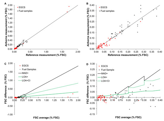
Figure 4.
Comparison of reference data from EGCS (in red ♦) and fuel samples (in black +) with the airborne measurement for the full FSC range; the perfect fit is visualized with a black line (x = y) (A). Comparison of reference data with airborne measurement for FSC values < 0.4% FSC (B). Modified B&A graph comparing the reference values with the airborne measurements for the total FSC range. The Limits of Agreement (LOA) are based on either the standard deviation or the relative standard deviation (the highest of the two applies), the confidence interval is added to the LOA in accordance with the CI as defined by the thresholds (LOA + CI) (C). Modified Bland Altman graph comparing the reference values with the airborne measurements for FSC values < 0.4% FSC (D).
The combined SDDiff was similar to that for the EGCS data (SDDiff = 0.004% FSC). The combined RSD was the same as that for the fuel samples (RSD = 3%). The combined Pearson correlation factor fell in between the individual correlation coefficients (r = 0.991). To validate the uncertainty levels used in the different color flag thresholds, the data were divided according the FSC level of the color flags. For the green flag, a minimum of 0.02% FSC was used to avoid errors due to the detection limit of either the sniffer sensor or the CEMS. This indicated that the SDdiff and RSD were below the applied uncertainty levels for all non-compliant thresholds, which was defined by the operational threshold (Tops) minus the sulfur limit (S) (Table 3).
A modified B&A graph is provided in Figure 4C,D. For these graphs, the difference in the two measurement methods were plotted against the average value together with: (1) the Limits of Agreement (+LOA); (2) the LOA added with the confidence interval (+LOA + CI); and (3) the maximum allowable difference (+MAD).
The standard B&A was modified using the RSD where this was larger than the SD. In addition, the different σ values were used for the CIs as defined in the thresholds instead of the standard 1.96 (with σ = 1 and a CI of 68% for yellow flags; σ = 1.96 and a CI of 95% for orange flags; and σ = 2.576 and a CI of 99% for red flags).
Finally, only the positive +LOA, +LOA + CI, and +MAD were visualized as the objective was to check for Type I errors and to evaluate the extent to which potential alerts have been sent for compliant vessels. This analysis showed that the +LOA + CI was well below the +MAD for all color flags. Moreover, all measurements were below the +MAD. Based on this analysis, it can be concluded that the effective uncertainty in the sniffer sensor is well below the calculated uncertainty used for the alert thresholds. It also demonstrates the existence of a proportional bias (higher alerts differed more than lower alerts), whereas this error remained well within the MAD. The systematic bias that was found in previous studies was, however, sufficiently removed with the application of the FSC correction [40].
3.4. NOx Validation
To validate NOx measurements, cooperation has been sought with the maritime industry. One Belgium engine manufacturer was willing to provide measurement data from CEMS systems installed on their OGVs. Unfortunately, these OGVs did not pass in the surveillance area of the Belgian coastguard aircraft during the airborne surveillance missions. NOx alerts of ships with destinations other than Belgium have also been reported by email to other European monitoring agencies using fixed sniffers. These fixed sniffer sensors are currently also measuring NOx but are not generating alerts such as those from the Belgian coastguard aircraft as they have no possibility to contact the OGV to request its Specific Fuel Consumption (SFC). Without this SFC information, the measurements have a large uncertainty. Moreover, the lack of EU regulations on NOx makes this a low priority for the inspection authorities of EU member states. For instance, in Germany, the BSH did take the initiative to follow up on some alerts for OGVs that were inbound to Germany. The comparison of these pairwise measurements is not as accurate as the comparison with EGCS or fuel samples as both sensors use the same measurement method. Nevertheless, for the concerned alerts, a relatively good comparison was found with the measurements in Germany (SDdiff = 5.55 g NOx/kWh and RSD = 22%), demonstrating that the NOx measurements used by fixed stations and airborne stations are useful for alerting high NOx non-compliant OGVs (Figure 5).
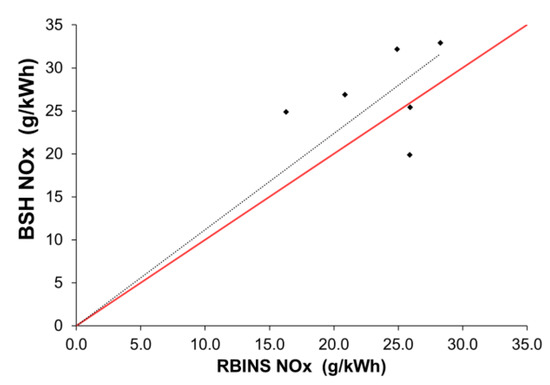
Figure 5.
Comparison of NOx measurements of RBINS (BE) with BSH (DE) (♦); the black dotted line represents the linear regression, and the red line represents a perfect correlation (x = y).
3.5. Cost Benefit Analysis
3.5.1. Comparison of Remote Compliance Monitoring with Port Inspections
An important aspect of the enforcement chain is the implementation cost. One of the incentives for the use of remote compliance monitoring is an improvement in the overall cost efficiency of the enforcement chain. The high labor effort is the most important cost factor in onboard inspections, followed by the cost of fuel sampling analyses by a certified laboratory (EUR 20–100) [43]. The total cost for the Belgian port inspection authorities amounted to approx. EUR 540 per FSC inspection in 2022. For NOx, no practical real-world emissions test is possible in port unless the OGV is equipped with a CEMS with a data logger. For these vessels (generally Tier III OGVs), the inspection effort can be compared to an inspection of an EGCS OGV. For the OGVs that are not equipped with a CEMS, the use of remote emission measurements can be considered as the only practical way to control real-world NOx emissions, as engine emission verification tests are too labor intensive to perform on a regular basis, and these tests are beyond the scope and capacity of port inspection authorities.
To calculate the cost per airborne measurement, a distinction is made between: (1) the net cost or the effective supplementary cost for RBINS for the sniffer flights per flight hour, including fuel costs, a breakdown of aircraft maintenance cost per flight hour, personal costs for the execution of the flights, amortization of sniffer hardware and software, gas calibrations, and sensor maintenance (Table S4) and (2) the full cost of the airborne operation program per hour, including overhead, among which are: all costs, including personal costs related to the program management and administration, fixed platform costs (such as insurance, aircraft stalling, and avionics data subscriptions), crew trainings, office computer hard- and software, and communication costs. The net cost can be regarded as the cost for RBINS to meet its national commitments, whereas the full cost is the “commercial” cost used when executing sniffer flights contracted by other countries. The overall cost per airborne FSC measurement was estimated to be EUR 122 for the net costs and EUR 188 for the full cost. From 2020 onward, both SO2 and NOx are measured, which resulted in a slightly lower number of inspections per hour. However, from that time, not one but two regulations were inspected for each OGV, thus decreasing the cost per inspected regulation to EUR 71 for the net cost and to EUR 109 for the gross cost (Table 4).
Table 4.
Cost efficiency calculation for different remote measurement techniques.
3.5.2. Comparison with Other Enforcement Methods
The outcome of the EU funded SCIPPER (Shipping Contributions to Inland Pollution Push for the Enforcement of Regulations) and CompMon (Compliance Monitoring) projects showed that airborne monitoring using fixed wing platforms is significantly more cost-effective than inspections in port and also when compared to airborne operations using medium range drones (vertical take-off and landing) and helicopters [31,43,91]. Based on the number of inspections and the costs of the operations in French waters, medium range drones are more expensive per inspection compared to onboard inspections. The reason why EU Member States prefer drones given their high cost per inspection lies in the EMSA RPAS (Remote Piloted Airborne Systems) program. The EU Member States are not charged for the deployment of the RPAS but only have to provide the facilities and the legal authorizations. By centralizing the RPAS operations, the prices quoted by EMSA are lower than if a Member State would implement this type of operations individually. It should be noted that the EMSA RPAS program only started in 2019, and with the experiences gained, the operational costs can be reduced in the coming years. The cost per inspection already showed a significantly reduced price of EUR 700–1000 per OGV according to the SCIPPER project outcome [31]. Fixed stations, on the other hand, are found to be the most cost-effective but have limited operational capabilities as they can only be used when shipping lanes pass close to the shore. The cost comparison made in the SCIPPER project demonstrated that this cost varied between EUR 20 and EUR 770 per OGV depending on the shipping density and the wind conditions at the location of the fixed station [31]. The cost for fixed stations used in this comparison is based on the cost of the fixed station operated by the TNO in the Netherlands on behalf of the Human Environment and Transport Inspectorate of the Ministry of Infrastructure and Water Management of the Netherlands (ILT) and the fixed station operated by Chalmers University in Denmark on behalf of the Danish Environmental Protection Agency (EPA). The operating cost and likewise the cost per inspection in the Netherlands in Rotterdam is substantially lower than the cost for the fixed station used in Denmark on the Great Belt Bridge due to the optimal wind orientation in Rotterdam, the higher maritime traffic density, and the easily accessible location.
3.5.3. Cost per Detected Violation
The cost efficiency of the airborne operations can also be expressed in the cost price per confirmed violation, which clearly demonstrated the added value of airborne monitoring (Table 5). The number of mandatory inspections according to the EU Directive is based on the number of port calls. For Belgium, the quota is 220 inspections with fuel sampling per year. However, as Belgium used remote monitoring, a reduction of 50% can be applied. For the non-compliance percentage of random fuel inspections, 2.7% was used. Therefore, 5.9 non-compliant OGVs would be identified. The total enforcement cost, in this case, would be EUR 118,000, thus resulting in a cost of EUR 20,000 per detected violation. In the case that port inspection authorities rely solemnly on airborne alerts, the confirmation rate would increase to 43%. With a reduced quota of 110 inspections, this would provide 47 confirmed non-compliant OGVs. To be able to provide sufficient alerts, the aircraft would need to operate for approx. 211.5 h. The resulting cost per confirmed violation would be EUR 8304, an improvement of almost 60%. However, the implementation of 211.5 flight hours would not be operationally or budgetary feasible. In addition, port inspection authorities also have to follow up on other types of alerts and cannot fit their planning completely based on the aircraft operations. With an allocated 70 flight hours per year, the aircraft would be able to provide approx. 1/3 of the alerts, resulting in a combined number of detected violations of 18.4 OGVs, which is already a drastic improvement. When looking at the total price per confirmed violation, this would amount to EUR 9622, which is an improvement of more than 50% compared to the base scenario without remote measurements. This would require all aircraft alerts to be followed up on by an onboard inspection, which for operational reasons may not always be possible. However, even with a follow-up rate of 80%, an improvement of 42% can be realized.
Table 5.
Cost calculation per confirmed violation.
4. Conclusions
Previous studies on airborne sniffer measurements, including recent sniffer improvements, have already demonstrated the reliability of airborne monitoring techniques for the enforcement of MARPOL Annex VI regulations 13 and 14. However, the effective improvement in enforcement of non-compliant OGVs remained unknown, and only limited field validation studies have been performed. This study makes the first ink between airborne sniffer measurements and the results of port inspections, which shows that about 46% of the alerts generated with the airborne monitoring are followed-up on by an inspection of the OGC, and about 43% of the alerts followed-up are confirmed by port inspection authorities. This study furthermore demonstrates that by including airborne alerts in the enforcement chain, the number of non-compliant detections in Belgian ports increased by 53%. When examining the sanctions issued by the FPS Mobility and Transport, 41% of all MARPOL Annex VI sanctions appear to be the result airborne alerts, which corresponds to 34% of the total amount of fines.
Compliance and follow-up on EGCS OGVs was also examined in this study. Due to the introduction of the Global Cap, the number of EGCS OGVs increased drastically, which coincided with a steep increase in the number of non-compliant EGCS-OGVs. The number of non-compliant EGCS OGVs was even higher than the number of non-compliant non-EGCS OGVs for the period of 2020 until 2022, while the frequency of observed EGCS OGVs in that period was only 30%. However, the onboard inspection of these OGVs poses major challenges for the port inspection authorities. The results clearly demonstrate that inspections of EGCS OGVs after airborne alerts improved the inspections drastically. Looking at sanctions, airborne alerts accounted for 2/3 of the sanctioned EGC-OGVs.
The results of this study also indicate that up to 80% of the observed potential non-compliant OGVs were not followed up or, if followed up, could not be confirmed with a fuel sample analysis. These results highlight the strong incentive to further explore the use of sniffer measurements as legal evidence for further tightening the MARPOL Annex VI enforcement chain. Therefore, a field validation was performed, demonstrating real-world measurement reliability. For that field validation, FSC measurements in the air are compared to FSC reference values from fuel samples and EGCS CEMS measurements. This analysis shows that the accuracy of the sensor is even better than expected.
For NOx, the situation is entirely different. Due to the lack of a mechanism for a practical compliance check by port inspection authorities in the IMO regulations and the absence of EU regulations in this regard, only very limited NOx inspections are carried out in ports. Moreover, these inspections are only based on documentary checks and cannot assess real-world NOx emissions and compliance, as would be the case with the use of remote measurements. In order for the real NOx emissions to be assessed by port inspection authorities, CEMS should become mandatory in international or European regulations. Consequently, the non-compliances observed by the aircraft remain only indicative and cannot be compared with the results of port inspections. In addition, no large-scale field validation could be conducted, but the comparison of high NOx alerts with other measurements in Germany have confirmed the Belgian NOx alerts and demonstrated the need for a more effective enforcement based on real-world emission measurements.
This study also analyzed the cost effectiveness of airborne monitoring and compared it to the cost of onboard inspections. Airborne measurements have been proven to be significantly cheaper than onboard inspections. Using airborne monitoring, the cost per detected violation can potentially be reduced by 40–50%. Although airborne monitoring is less cost-effective than fixed stations per inspection, airborne measurements provide more flexibility as they can operate over a full ECA. Airborne monitoring also provides more opportunities to obtain legal evidence, as it is possible to collect multiple measurements, dramatically increasing the reliability of non-compliance alerts.
This study has also demonstrated that airborne measurements can play a first role in the enforcement chain as scientifically proven sound legal evidence for further legal actions. The field validation performed in this study can be regarded as an initial assessment, while further large-scale field validation experiments for compliance with both SO2 and NOx emissions from a legal evidence perspective remain highly advisable. These large-scale field validation experiments require a substantial organization and are therefore best organized in the framework of an EU-funded project with the participation of other EU Member States.
Supplementary Materials
The following supporting information can be downloaded at: https://www.mdpi.com/article/10.3390/atmos14040623/s1, Figure S1. Emission Control Area (ECA) as defined by MARPOL Annex VI (Upper). Limits on the fuel content of marine fuels according to the MARPOL Annex VI regulation 14 (Middle). NOx emission limits according to MARPOL Annex VI Regulation 13 (Lower). Figure S2. Boxplot comparison of results of fuel samples executed without airborne alerts and the results of the airborne measurements, with minimum, maximum median, average (♦), and 25 and 75 percentiles (Upper). Comparison of the results from the fuel sample analysis executed by Belgian port inspection authorities initiated without and with the use of airborne alerts (Lower). Figure S3. Number OGVs and relative amount of the 20 most observed ports of destination (Upper) and country of destination (Lower). Figure S4. Monthly average, median, and non-compliance values for FSC (A) and NOx (B). Normalized values for median and non-compliance for FSC (C) and NOx (D) compared to the normalized monthly values for T and RH. The months of January, February, and December were not included for FSC, and additionally, the month of November was not included for NOx due to the low number of measurements for these months. Table S1. Emission ratios for EGCS systems Table S2. Test cycles and weighting factors according to the NOx Technical code. Table S3. R2 values for the linear regression between the monthly values for average FSC, median FSC, FSC non-compliance, average NOx, median NOx, NOx non-compliance, relative humidity (RH), and temperature (T). Table S4. Cost breakdown of the Belgian Sniffer program 2016–2022.
Author Contributions
Conceptualization, W.V.R.; data curation, W.V.R.; formal analysis, W.V.R.; funding acquisition, W.V.R., K.S. and R.S.; investigation, W.V.R., J.-B.M., A.V.N., K.S. and B.V.R.; methodology, W.V.R.; project administration, W.V.R. and K.S.; resources, W.V.R., J.-B.M., A.V.N., K.S. and B.V.R.; software, W.V.R.; validation, W.V.R.; visualization, W.V.R.; writing—original draft, W.V.R.; writing—review and editing, W.V.R., J.-B.M., A.V.N., K.S., B.V.R., R.S. and F.M. All authors have read and agreed to the published version of the manuscript.
Funding
The sniffer has been partially funded by the European Commission through the Connecting Europe Facility (CEF) program (2014 EU TM 0546 S). The NOx sensor has been funded by the Belgian minister in charge of the North Sea. The development of the upload script and the update of the mission management system on board for reporting alerts has been funded by the Environmental Compensation Fund of the Federal Public Service for the Environment.
Institutional Review Board Statement
Not applicable.
Informed Consent Statement
Not applicable.
Data Availability Statement
The airborne monitoring dataset is available at: https://doi.org/10.24417/bmdc.be:dataset:2687.
Acknowledgments
The authors wish to thank the pilots of the Belgian Defense Airforce Component: Geert Present, Alexander Vermeire, Pieter Janssens, and Dries Noppe for the safe and highly professional performance of the surveillance flights. The ministry of the North Sea is gratefully acknowledged for funding the NOx sensor. The Federal Public Service Environment is gratefully appreciated for funding the Thetis-EU upload tool and the upgrade of the mission management software on board the coastguard aircraft. Acknowledgment to the European Directorate General for Mobility and Transport (DG-MOVE) for funding the sniffer sensor. The European Maritime Safety Agency (EMSA) and Nabil Youdjou are gratefully acknowledged for setting up the automatic upload protocol for remote OGV emission measurements. Acknowledgment to the Human Environment and Transport Inspectorate of the Ministry of Infrastructure and Water Management of the Netherlands (ILT) for their approval to use the monitoring data collected by RBINS in charge of ILT. The authors wish to thank Christophe Swolfs, Steven Werkers, and Bart Colaers from the Federal Public Service for Mobility and Transport for their help with the interpretation of the international regulations and Belgian national laws, the provision of the port inspection data, and the collection of reference fuel samples. The authors wish to thank Albina Mjaki from the Brussels Institute of Environment (BIM) for her help with the calibration of the reference gasses. The authors wish to thank Andreas Weigelt of the German Federal Maritime and Hydrographic Agency (BSH) for providing NOx measurement data. The authors wish to thank Johan Mellqvist and Alexander A. Vladimir Conde from Chalmers University of Technology for their continuing help in maintaining and improving the sniffer sensor. Rebecca Gualandi is gratefully appreciated for the proofreading.
Conflicts of Interest
The authors declare that they have no known competing financial interest or personal relationships that could have appeared to influence the work reported in this paper.
References
- IMO. Protocol of 1997 to Amend the International Convention for the Prevention of Pollution from Ships of 2 November 1973, as Modified by the Protocol of 17 February 1978; International Maritime Organization: London, UK, 1997. [Google Scholar]
- MEPC. RESOLUTION MEPC.259(68) 2015 Guidelines for Exhaust Gas Cleaning Systems; Marine Environment Protection Committee; International Maritime Organization: London, UK, 2015; pp. 1–23. [Google Scholar]
- Endres, S.; Maes, F.; Hopkins, F.; Houghton, K.; Mårtensson, E.M.; Oeffner, J.; Quack, B.; Singh, P.; Turner, D. A New Perspective at the Ship-Air-Sea-Interface: The Environmental Impacts of Exhaust Gas Scrubber Discharge. Front. Mar. Sci. 2018, 5, 139. [Google Scholar] [CrossRef]
- MEPC. RESOLUTION MEPC.132(53) Amendments to the Annex of the Protocol of 1997 to Amend the International Convention for the Prevention of Pollution from Ships, 1973, as Modified by the Protocol of 1978 Relating Thereto; Marine Environmental Protection Committee; International Maritime Organization: London, UK, 2005; pp. 1–16. [Google Scholar]
- MEPC. RESOLUTION MEPC.194(61) Amendments to the Annex of the Protocol of 1997 to Amend the International Convention for the Prevention of Pollution from Ships, 1973, as Modified by the Protocol of 1978 Relating Thereto; Marine Environment Protection Committee; International Maritime Organization: London, UK, 2010; pp. 1–11. [Google Scholar]
- IMO. Annex VI Regulations for the Prevention of Air Pollution from Ships; International Maritime Organization: London, UK, 2008. [Google Scholar]
- MEPC. RESOLUTION MEPC.280(70) Effective Date of Implementation of the Fuel Oil Standard in Regulation 14.1.3 of MARPOL Annex VI; Marine Environment Protection Committee; International Maritime Organization: London, UK, 2016; pp. 1–3. [Google Scholar]
- MEPC. RESOLUTION MEPC.305(73) Amendments to the Annex of the Protocol of 1997 to Amend the International Convention for the Prevention of Pollution from Ships, 1973, as Modified by the Protocol of 1978 Relating Thereto; Marine Environment Protection Committee; International Maritime Organization: London, UK, 2018; pp. 1–5. [Google Scholar]
- EU. Council Directive 1999/32/EC of 26 April 1999 Relating to a Reduction in the Sulphur Content of Certain Liquid Fuels and Amending Directive 93/12/EEC.; Council of the European Union: Brussels, Belgium, 1999; pp. 13–18.
- EU. Directive 2005/33/EC of the European Parliament and of the Council of 6 July 2005; European Parliament: Strasbourg, French, 2005.
- EU. Commission Implementing Decision (EU.) 2015/253-of 16 February 2015-Laying down the Rules Concerning the Sampling and Reporting under Council Directive 1999/32/EC as Regards the Sulphur Content of Marine Fuels; The European Commission: Brussels, Belgium, 2015; pp. 45–59.
- EU. Directive (EU.) 2016/802 of the European Parliament and of the Council of 11 May 2016 Relating to a Reduction in the Sulphur Content of Certain Liquid Fuels; The European Parliament and the Council of the European Union: Brussels, Belgium, 2016; pp. 58–78.
- Royal Decree. Koninklijk Besluit Inzake MiliEU. Vriendelijke Scheepvaart; Belgisch Staatsblad: Brussels, Belgium, 2020; pp. 63339–63386.
- MEPC. RESOLUTION MEPC.202(62) Amendments to the Annex of the Protocol of 1997 to Amend the International Convention for the Prevention of Pollution from Ships, 1973, as Modified by the Protocol of 1978 Relating Thereto (Designation of the United States Caribbean Sea Emission Control Area and Exemption of Certain Ships Operating in the North American Emission Control Area and the United States Caribbean Sea Emission Control Area under Regulations 13 and 14 and Appendix VII of MARPOL Annex VI); Marine Environment Protection Committee; International Maritime Organization: London, UK, 2011; pp. 2–13. [Google Scholar]
- MEPC. RESOLUTION MEPC.70/5/Rev.1 Proposal to Designate the North Sea as an Emission Control Area for Nitrogen Oxides (Submitted by Belgium et al.); Marine Environment Protection Committee; International Maritime Organization: London, UK, 2016; pp. 1–71. [Google Scholar]
- MEPC. CIRCULAR MEPC.1/Circ.778/Rev.3 List of Special Areas, Emission Control Areas and Particularly Sensitive Sea Areas; Marine Environmental Protection Committee; International Maritime Organization: London, UK, 2018; pp. 1–5. [Google Scholar]
- Heywood, J. Internal Combustion Engine Fundamentals Second Edition, 2nd ed.; McGraw-Hill Education Ltd: London, UK, 2018. [Google Scholar]
- IMO. NOx Technical Code 2008—Amendments to the Technical Code on Control of Emission of Nitrogen Oxides from Marine Diesel Engines (NOx Technical Code 2008); International Maritime Organisation: London, UK, 2008. [Google Scholar]
- MEPC. CIRCULAR MEPC.1/Circ.679 Guidelines for the Application of the NOx Technical Code Relative to Certification and Amendments of Tier I Engines; Marine Environmental Protection Committee; International Maritime Organization: London, UK, 2009. [Google Scholar]
- MEPC. RESOLUTION MEPC.176(58) Amendments to the Annex of the Protocol of 1997 to Amend the International Convention for the Prevention of Pollution from Ships, 1973, as Modified by the Protocol of 1978 Relating Thereto (Revised MARPOL Annex VI); Marine Environment Protection Committee; International Maritime Organization: London, UK, 2008; pp. 1–46. [Google Scholar]
- EU. Revision of the Directive 2005/35/EC on Ship-Source Pollution and on the Introduction of Penalties for Infringements; The European Parliament and the Council of the European Union: Brussels, Belgium, 2022.
- Bloss, M. EU.-CO2-Handel Für Die Schiffahrt Kommt. 2022. Available online: https://michaelbloss.eu/de/presse/themenhintergrund/eu-co2-handel-fuer-die-schiffahrt-kommt (accessed on 22 December 2022).
- EU. Fit for 55 in 2030: Parliament Wants a More Ambitious Emissions Trading System; The European Parliament and the Council of the European Union: Brussels, Belgium, 2022. [Google Scholar]
- EU. Ractiv. EU. Agrees Carbon Market Overhaul in Bid to Hit 2030 Climate Goal; The European Parliament and the Council of the European Union: Brussels, Belgium, 2022.
- European Commission. Proposal for a Directive of the European Parliament and of the Council Amending Directive 2003/87/EC Establishing a System for Greenhouse Gas Emission Allowance Trading within the Union, Decision (EU.) 2015/1814 Concerning the Establishment and Operation of a Market Stability Reserve for the Union Greenhouse Gas Emission Trading Scheme and Regulation (EU.) 2015/757; The European Parliament and the Council of the European Union: Brussels, Belgium, 2021.
- Council of the European Union. Proposal for a Directive of the European Parliament and of the Council Amending Directive 2003/87/EC Establishing a System for Greenhouse Gas Emission Allowance Trading within the Union, Decision (EU.) 2015/1814 Concerning the Establishment and Operation of a Market Stability Reserve for the Union Greenhouse Gas Emission Trading Scheme and Regulation (EU.) 2015/757; The Council of the European Union: Brussels, Belgium, 2022.
- EU. Amendments Adopted by the European Parliament on 22 June 2022 on the Proposal for a Directive of the European Parliament and of the Council Amending Directive 2003/87/EC Establishing a System for Greenhouse Gas Emission Allowance Trading within the Union, Decision (EU.) 2015/1814 Concerning the Establishment and Operation of a Market Stability Reserve for the Union Greenhouse Gas Emission Trading Scheme and Regulation (EU.) 2015/757 (COM(2021)0551-C9-0318/2021-2021/0211(COD)); European Parliament: Brussels, Belgium, 2022.
- Repka, S.; Erkkilä-Välimäki, A.; Jonson, J.E.; Posch, M.; Törrönen, J.; Jalkanen, J.P. Assessing the costs and environmental benefits of IMO regulations of ship-originated SOx and NOx emissions in the Baltic Sea. Ambio 2021, 50, 1718–1730. [Google Scholar] [CrossRef] [PubMed]
- Viana, M.; Rizza, V.; Tobías, A.; Carr, E.; Corbett, J.; Sofiev, M.; Karanasiou, A.; Buonanno, G.; Fann, N. Estimated health impacts from maritime transport in the Mediterranean region and benefits from the use of cleaner fuels. Environ. Int. 2020, 138, 105670. [Google Scholar] [CrossRef] [PubMed]
- Sofiev, M.; Winebrake, J.J.; Johansson, L.; Carr, E.W.; Prank, M.; Soares, J.; Vira, J.; Kouznetsov, R.; Jalkanen, J.P.; Corbett, J.J. Cleaner fuels for ships provide public health benefits with climate tradeoffs. Nat. Commun. 2018, 9, 406. [Google Scholar] [CrossRef] [PubMed]
- Verbeek, R.; Van Dinther, D.; Mamarik, S.; Grigoriadis, A.; Weigelt, A.; Van Vliet, J.; Smyth, T.; Deakin, A.; Irjala, M. SCIPPER Project D5.3 Cost-Effectiveness of Different Approaches for Compliance; The European Parliament and the Council of the European Union: Brussels, Belgium, 2022. [Google Scholar]
- Corbett, J.J.; Fischbeck, P.S. Emissions from Ships. Science 1997, 278, 823–824. [Google Scholar] [CrossRef]
- Gillis, M. Let’s Play? An Examination of the ‘Level Playing Field’ in EU. Free Trade Agreements. J. World Trade 2021, 55, 715–740. [Google Scholar] [CrossRef]
- Van Miert, K. What Does a Level Playing Field Mean in the Global Economy? In Proceedings of the DAVOS World Economic Forum, Davos, Switzerland, 30 January 1998; Available online: https://ec.EU.ropa.EU./competition/speeches/text/sp1998_031_en.html (accessed on 15 December 2022).
- EU. Trade Defence—Ensuring a Level Playing Field; European Parliament: Brussels, Belgium, 2010.
- WHO. World Trade Report 2022-Climate Change and International Trade; World Health Organization: Geneva, Switzerland, 2022.
- Berg, N.; Mellqvist, J.; Jalkanen, J.P.; Balzani, J. Ship Emissions of SO2 and NO2: DOAS Measurements from Airborne Platforms. Atmos. Meas. Tech. 2012, 5, 1085–1098. [Google Scholar] [CrossRef]
- Balzani Lööv, J.M.; Alfoldy, B.; Gast, L.F.L.; Hjorth, J.; Lagler, F.; Mellqvist, J.; Beecken, J.; Berg, N.; Duyzer, J.; Westrate, H.; et al. Field Test of Available Methods to Measure Remotely SOx and NOx Emissions from Ships. Atmos. Meas. Tech. 2014, 7, 2597–2613. [Google Scholar] [CrossRef]
- Van Roy, W.; Schallier, R.; Van Roozendael, B.; Scheldeman, K.; Van Nieuwenhove, A.; Maes, F. Airborne Monitoring of Compliance to Sulfur Emission Regulations by Ocean-Going Vessels in the Belgian North Sea Area. Atmos. Pollut. Res. 2022, 13. [Google Scholar] [CrossRef]
- Van Roy, W.; Van Nieuwenhove, A.; Scheldeman, K.; Van Roozendael, B.; Schallier, R.; Mellqvist, J.; Maes, F. Measurement of Sulfur-Dioxide Emissions from Ocean-Going Vessels in Belgium Using Novel Techniques. Atmosphere 2022, 13, 1756. [Google Scholar] [CrossRef]
- Van Roy, W.; Scheldeman, K.; Van Roozendael, B.; Van Nieuwenhove, A.; Schallier, R.; Vigin, L.; Maes, F. Airborne Monitoring of Compliance to NOx Emission Regulations from Ocean-Going Vessels in the Belgian North Sea. Atmos. Pollut. Res. 2022, 13, 101518. [Google Scholar] [CrossRef]
- Beecken, J.; Irjala, M.; Weigelt, A.; Conde, V.; Mellqvist, J.; Proud, R.; Deakin, A.; Knudsen, B.; Timonen, H.; Sundström, A.-M.; et al. SCIPPER Project D2.1 Review of Available Remote Systems for Ship Emission Measurements; The European Parliament and the Council of the European Union: Brussels, Belgium, 2019. [Google Scholar]
- CompMon. Compliance monitoring pilot for Marpol Annex VI (CompMon), Connection European Facility, 2014-EU.-TM-0546-S; The European Parliament and the Council of the European Union: Brussels, Belgium, 2016.
- Mellqvist, J.; Conde, V. SCIPPER Project D2.2 Prototype of Revised Sniffer Type of Remote Monitor Demonstrator; The European Parliament and the Council of the European Union: Brussels, Belgium, 2022. [Google Scholar]
- Mellqvist, J.; Ekholm, J.; Salo, K.; Beecken, J. Identification of Gross Polluting Ships to Promote a Level Playing Field withing the Shipping Sector; Swedish National Road and Transport Research Institute: Linköping, Sweden, 2014. [Google Scholar]
- Beecken, J.; Mellqvist, J.; Salo, K.; Ekholm, J.; Jalkanen, J.-P. Airborne Emission Measurements of SO2, NOx and Particles from Individual Ships Using a Sniffer Technique. Atmos. Meas. Tech. 2014, 7, 1957–1968. [Google Scholar] [CrossRef]
- Beecken, J.; Mellqvist, J.; Salo, K.; Ekholm, J.; Jalkanen, J.-P.; Johansson, L.; Litvinenko, V.; Volodin, K.; Frank-Kamenetsky, D.A. Emission factors of SO2, NOx and particles from ships in Neva Bay from ground-based and helicopter-borne measurements and AIS-based modelling. Atmos. Chem. Phys. 2015, 15, 5229–5241. [Google Scholar] [CrossRef]
- Alföldy, B.; Lööv, J.B.; Lagler, F.; Mellqvist, J.; Berg, N.; Beecken, J.; Weststrate, H.; Duyzer, J.; Bencs, L.; Horemans, B.; et al. Measurements of air pollution emission factors for marine transportation in SECA. Atmos. Meas. Tech. 2013, 6, 1777–1791. [Google Scholar] [CrossRef]
- Duyzer, J.H.; Weststrate, J.H. Measurements of Fuel Sulphur Content by Measurements in the Plume; Technical report; TNO: Apeldoorn, The Netherlands, 2015. [Google Scholar]
- Van Dinther, D.; Duyzer, J.H.; De Bie, S.; Moerman, M.M.; Lollinga, J.P.; Maarschalkerweerd, T.V.P. Measurements of Emission Factors of Nitrogen Oxides of Seagoing Vessels in the Port of Rotterdam; TNO: Apeldoorn, The Netherlands, 2022. [Google Scholar]
- Weigelt, A. Sulphur emission compliance monitoring of ships in German waters—results from five years of operation. In Shipping and the Environment, Symposium on Scenarios and Policy Options for Sustainable Shipping (POL) Goteborg; BSH: Hamburg, Germany, 2019. [Google Scholar]
- Weigelt, A.; Thomsen, C.; Bliemeister, J. German Ship Emission Monitoring Network Remote Emission Measurements to Support MARPOL Annex VI Compliance Monitoring; BSH: Hamburg, Germany, 2021. [Google Scholar]
- Behrens, L.; Kattner, L.; Mathieu-Üffing, B.; Krause, K.; Meier, A.; Ochmann, S.; Ostendorf, M.; Peters, E.; Richter, A.; Schönhardt, A.; et al. Measurements of Shipping Emissions in the Marine Troposphere-Phase 2: Further Development of Remote Sensing Methods and Implementation into an Operational Network MeSmarT-II. Bremen. 2020. Available online: https://www.bsh.de/DE/PUBLIKATIONEN/_Anlagen/Downloads/Projekte/MeSmarT/Final_Report.html (accessed on 22 December 2022).
- Mellqvist, J.; Beecken, J.; Conde, V.; van Dinther, D.; Duyzer, J.; Griesel, S.; Irjala, M.; Knudsen, B.; Knudsen, J.; Moerman, M.; et al. SCIPPER Project D2.3—Quality assurance of remote monitoring systems and harmonised reporting; The European Parliament and the Council of the European Union: Brussels, Belgium, 2022. [Google Scholar]
- EMSA. RPAS Service Ship Emission Monitoring; European Maritime Safety Agency: Lisbon, Portugal, 2022.
- Enge, S.E. Sulphur Expert Meeting 2018. The Use of Drones for Sulphur Controls, Antwerp. 2018. [Google Scholar]
- Duyzer, J.; Hollander, K.; Marita, V.; Verhagen, H.; Hilbrand, W.; Hensen, A.; Kraai, A.; Kos, G. Assessment of Emissions of PM and NOx of Sea Going Vessels by Field Measurements; TNO: Apeldoorn, The Netherlands, 2007. [Google Scholar]
- Lööv, J.M.B.; Alfoldy, B.; Beecken, J.; Berg, N.; Berkhout, A.J.C.; Duyzer, J.; Gast, L.F.L.; Hjorth, J.; Jalkanen, J.P.; Lagler, F.; et al. Field test of available methods to measure remotely SO2 and NOx emissions from ships. Atmos. Meas. Tech. Discuss. 2013, 6, 9735–9782. [Google Scholar] [CrossRef]
- Au, C.N.; Delea, C.; Schneider, V.E.; Oeffner, J.; Jahn, C. A Web-oriented Architecture for Deploying Multiple Unmanned Vehicles as a Service. TransNav. Int. J. Mar. Navig. Saf. Sea Transp. 2021, 15, 155–162. [Google Scholar] [CrossRef]
- Sokhi, R.S.; Moussiopoulos, N.; Baklanov, A.; Bartzis, J.; Coll, I.; Finardi, S.; Friedrich, R.; Geels, C.; Grönholm, T.; Halenka, T.; et al. Advances in air quality research—current and emerging challenges. Atmos. Chem. Phys. 2022, 22, 4615–4703. [Google Scholar] [CrossRef]
- Smyth, T.; Bell, T.; Fishwick, J.; Yang, M. Reportingship Exhaust Gas Emissions Using Automatic Identification System Technology; Plymouth Marine Laboratory: Plymouth, UK, 2019; Unpublished report. [Google Scholar]
- Prata, A.J. Measuring SO2 ship emissions with an ultraviolet imaging camera. Atmos. Meas. Tech. 2014, 7, 1213–1229. [Google Scholar] [CrossRef]
- Walden, J.; Pirjola, L.; Laurila, T.; Hatakka, J.; Pettersson, H.; Walden, T.; Jalkanen, J.-P.; Nordlund, H.; Truuts, T.; Meretoja, M.; et al. Measurement report: Characterization of uncertainties in fluxes and fuel sulfur content from ship emissions in the Baltic Sea. Atmos. Chem. Phys. 2021, 21, 18175–18194. [Google Scholar] [CrossRef]
- Karjalainen, P.; Teinilä, K.; Kuittinen, N.; Aakko-Saksa, P.; Bloss, M.; Vesala, H.; Pettinen, R.; Saarikoski, S.; Jalkanen, J.P.; Timonen, H. Real-world particle emissions and secondary aerosol formation from a diesel oxidation catalyst and scrubber equipped ship operating with two fuels in a SECA area. Environ. Pollut. 2022, 292, 118278. [Google Scholar] [CrossRef]
- Royal Decree. Wet Tot Invoering van Het Belgisch Scheepvaartwetboek; Belgisch Staatsblad: Gent, Belgium, 2019; pp. 75432–75808.
- MEPC. CIRCULAR MEPC.1/Circ.864/Rev.1 Guidelines for on Board Sampling for the Verification of the Sulphur Content of the Fuel Oil Used on Board Ships; Marine Environment Protection Committee; International Maritime Organization: London, UK, 2019. [Google Scholar]
- Belgisch Staatsblad. Wet van 25 December 2016 Tot Vaststelling van Administratieve Geldboetes van Toepassing in Geval van Inbreuken Op de Scheepvaartwetten; Belgisch Staatsblad: Gent, Belgium, 2017; pp. 3439–3446. [Google Scholar]
- EMSA. Thetis-EU. 2022. Available online: Https://Portal.Emsa.europa.EU./Web/Thetis-EU (accessed on 16 December 2022).
- MEPC. RESOLUTION MEPC.184(59) Guidelines for Exhaust Gas Cleaning Systems; Marine Environment Protection Committee; International Maritime Organization: London, UK, 2009; pp. 1–26. [Google Scholar]
- Devore, J.; Berk, K.; Carlton, M. Modern Mathematical Statistics with Applications, 3rd ed.; Springer: Berlin/Heidelberg, Germany, 2011. [Google Scholar]
- Gardner, M.J.; Altman, D.G. Estimating with Confidence. BMJ 1988, 296, 1210–1211. [Google Scholar] [CrossRef] [PubMed]
- Sprinthall, R.C. Basic Statistical Analysis, 9th ed.; Pearson: London, UK, 2011. [Google Scholar]
- Martin Bland, J.; Altman, D.G. Statistical Methods for Assessing Agreement Between two Methods of Clinical Measurement. Lancet 1986, 327, 307–310. [Google Scholar] [CrossRef]
- Altman, D.G.; Bland, J.M. Measurement in Medicine: The Analysis of Method Comparison Studies. Statistician 1983, 32, 307. [Google Scholar] [CrossRef]
- EMSA. COVID-19 Impact on Shipping; European Maritime Safety Agency: Lisbon, Portugal, 2021.
- Port State Control Dealing with the Pandemic-Annual Report 2020; Paris MoU: Den Hague, The Netherlands, 2021.
- Airborne Monitoring of Sulphur Emissions from Ships in Danish Waters, 2019 Campaign Results; Explicit ApS: Lyngby-Taarbæk, Denmark, 2020.
- Airborne Monitoring of Sulphur Emissions from Ships in Danish Waters, 2020 Campaign Results; Explicit ApS: Lyngby-Taarbæk, Denmark, 2021.
- Airborne Monitoring of Sulphur Emissions from Ships in Danish Waters, 2018 Campaign Results; Explicit ApS: Lyngby-Taarbæk, Denmark, 2019.
- Airborne Monitoring of Sulphur Emissions from Ships in Danish Waters: 2017 Campaign Results; Danish Environmental Protection Agency: Lyngby-Taarbæk, Denmark, 2018.
- Airborne Monitoring of Sulphur Emissions from Ships in Danish Waters: 2021 Campaign Results; Danish Environmental Protection Agency: Lyngby-Taarbæk, Denmark, 2022.
- Mellqvist, J.; Conde, V. Surveillance of Sulfur Fuel Content in Ships at the Great Belt Bridge 2018; The Danish Environmental Protection Agency: Odense, Denmark, 2019.
- Mellqvist, J.; Conde, V. Surveillance of Sulfur Fuel Content in Ships at the Great Belt Bridge 2019; The Danish Environmental Protection Agency: Odense, Denmark, 2020. [Google Scholar]
- Mellqvist, J.; Beecken, J.; Conde, V.; Ekholm, J. Surveillance of Sulfur Emissions from Ships in Danish Waters 2017; The Danish Environmental Protection Agency: Odense, Denmark, 2018.
- Mellqvist, J.; Beecken, J.; Conde, V.; Van Dinther, D.; Duyzer, J.; Griesel, S.; Irjala, M.; Knudsen, B.; Knudsen, J.; Moerman, M.; et al. THE SCIPPER PROJECT Shipping Contributions to Inland Pollution Push for the Enforcement of Regulations; The European Parliament and the Council of the European Union: Brussels, Belgium, 2022. [Google Scholar]
- Van Roy, W.; Scheldeman, K. Compliance Monitoring Pilot for MARPOL Annex VI, Results MARPOL Annex VI Monitoring Report Belgian Sniffer Campaign 2016; The European Parliament and the Council of the European Union: Brussels, Belgium, 2016. [Google Scholar]
- Van Roy, W.; Scheldeman, K. Compliance Monitoring Pilot for MARPOL Annex VI, Best Practices Airborne MARPOL Annex VI Monitoring; The European Parliament and the Council of the European Union: Brussels, Belgium, 2016. [Google Scholar]
- Majamäki, E.; Jalkanen, J.-P. SCIPPER Project D4.2 Updated Inventories Onregional Shipping Activityand Port Regions; The European Parliament and the Council of the European Union: Brussels, Belgium, 2021. [Google Scholar]
- The Scipper Project. SCIPPER Project Finds High Nitrogen Oxides Emissions of Tier III Vessels from Remote Measurements in North European Seas; The European Parliament and the Council of the European Union: Brussels, Belgium, 2023. [Google Scholar]
- Winnes, H.; Fridell, E.; Verbeek, R.; Duyzer, J.; Weigelt, A.; Mamarikas, S.; Ntziachristos, L. SCIPPER Project D5.1 Gaps in Current Emission Enforcement Regulations and Impacts to Real-World Emissions; The European Parliament and the Council of the European Union: Brussels, Belgium, 2019. [Google Scholar]
- SCIPPER. 2023. Available online: https://www.scipper-project.EU (accessed on 30 January 2023).
- Grigoriadis, A.; Mamarikas, S.; Ntziachristos, L. Emission performance of major ship classes: An estimation based on a new set of emission factors and realistic activity profile data. IOP Conf. Ser. Earth Env. Sci. 2021, 899, 012005. [Google Scholar] [CrossRef]
- Knudsen, B.; Lallana, A.L.; Ledermann, L. NOx Emissions from Ships in Danish Waters Assessment of Current Emission Levels and Potential Enforcement Models; The Danish Environmental Protection Agency: Odense, Denmark, 2022.
- Asad, U.; Kelly, C.; Wang, M.; Tjong, J. Effects of Intake Air Humidity on the NOX Emissions and Performance of a Light-Duty Diesel Engine. In Proceedings of the ASME 2012 Internal Combustion Engine Division Fall Technical Conference, American Society of Mechanical Engineers, Vancouver, BC, Canada, 23–26 September 2012; pp. 235–242. [Google Scholar] [CrossRef]
- Agentschap Maritieme Dienstverlening en Kust. 2019. Available online: https://www.kustweerbericht.be/nl/rapporten (accessed on 2 May 2022).
- Ship and Bunker. Scrubber Equipped Tonnage Now 30% of Boxship Capacity. 2021. Available online: Https://Shipandbunker.Com/News/World/867193-Scrubber-Equipped-Tonnage-Now-30-of-Boxship-Capacity (accessed on 15 June 2022).
- MEPC. RESOLUTION MEPC.79/INF.4 Inspections of Exhaust Gas Cleaning Systems—First Experiences; Marine Environmental Protection Committee; International Maritime Organization: London, UK, 2022. [Google Scholar]


Disclaimer/Publisher’s Note: The statements, opinions and data contained in all publications are solely those of the individual author(s) and contributor(s) and not of MDPI and/or the editor(s). MDPI and/or the editor(s) disclaim responsibility for any injury to people or property resulting from any ideas, methods, instructions or products referred to in the content. |
© 2023 by the authors. Licensee MDPI, Basel, Switzerland. This article is an open access article distributed under the terms and conditions of the Creative Commons Attribution (CC BY) license (https://creativecommons.org/licenses/by/4.0/).