Abstract
Pollution in urban areas has been one of the most relevant problems of the last decade since it represents a threat to public health. Specifically, particulate matter (PM2.5) is a pollutant that causes serious health complications, such as heart and lung diseases. Centers for monitoring contaminants and climatic variables have been established to adopt measures to control the consequences of high levels of air pollution. However, these monitoring centers sometimes make decisions when pollution levels are already harmful to health, which may be related to sensor miscalibration and failures. This study presents a PM2.5 prediction system based on a state-space model—developed with real data from 2019—plus a Kalman filter to improve the prediction. The system was subsequently validated using real data captured in 2018 in Valle de Aburrá. Therefore, this is an important first step towards a more robust PM diagnosis and prediction system in the presence of false and mismatched data in the measurement.
1. Introduction
The exponential growth of the urban population has increased the demand for services related to industries and transportation systems, as well as the use of hydrocarbon resources. This has, in turn, caused urban areas to experience significant levels of air pollution. For instance, Valle de Aburrá in Colombia—an urban agglomeration made up of ten municipalities—faces many air quality issues due to an increase in the emission of polluting gases (e.g., CO, NO2, SO2, and O3) and particles smaller than 10 µm (PM10) or 2.5 µm (PM2.5) [1]. These pollutants, when released into the atmosphere (mainly by automobiles and industries), remain suspended in the air and are typically carried by the wind. However, during the change in season, the wind cannot carry the pollution away. This is because the topography of Valle de Aburrá and the low atmospheric turbulence caused by the change in season prevent the wind currents, and, therefore, the contamination, from moving out of the area. This phenomenon can occur two or three times a year.
The Institute of Hydrology, Meteorology and Environmental Studies (IDEAM) and the Aburrá Valley Early Warning System (SIATA) are two of the entities in charge of monitoring pollutants in the Aburrá Valley. They collect and analyze monitoring data using air quality variables to improve control policies and strategies. In particular, to prevent and mitigate air pollution, they use monitoring systems that measure pollutants (e.g., PM10, PM2.5, CO, NO, NO2, SO2, and O3) and meteorological variables (e.g., pressure, temperature, humidity, and wind speed), which serve as input to understand how climate affects concentrations of pollutants [2]. SIATA is comparable to monitoring systems such as the Urban Air Quality Management Capabilities Index (CECA) developed by the World Health Organization (OMS), which oversees coordinating the databases for air quality control and data on issues related to air quality, facilitates the exchange of information on air quality between countries, and expands the distribution of documents on monitoring and management of air quality in Latin America [3]. In the same way, the AIREBASE, which manages and administers information related to air quality but within the European Union, is also developed and monitored by the OMS [4]. Nonetheless, since these monitoring systems take information from the environment, they are faced with a large amount of interference (measurement noise). In addition, like any other measurement system, they need periodic maintenance and adjustment. Hence, the information obtained from these systems on the behavior of pollutants and the various meteorological variables may be distorted, resulting in the delivery of spurious or incomplete data [5].
In light of the above, different strategies have been developed worldwide to predict the behavior of contamination, especially PM2.5, which is the most harmful pollutant to human health [6]. For example, in study [7], a computational intelligence technique based on a recurrent neural network (RNN) and the particle swarm optimization algorithm was designed to predict the concentration of six air pollutants. The proposed technique includes two stages: (i) data collection from multiple stations and (ii) data preprocessing, which involves (a) separating each station with an independent approach, (b) handling missing values, and (c) normalizing the dataset to the range of (0, 1) using the MinMaxScalar method. In a previous study, a neural network model was developed to predict the concentrations of pollutants in India for 2013 using datasets containing meteorological data and concentrations of respirable suspended particulate matter (RSPM) and suspended particulate matter (SPM) from 2009 to 2013 [8]. The developed model helps to provide alerts and early warnings for air quality management. In another study, an innovative strategy to predict the amount of PM2.5 using images was proposed by [9]. According to such a strategy, by means of a neural network fed with images of polluted and unpolluted areas, a given model can be trained to detect the level of pollution in an area in real-time.
Similarly, models to predict particulate matter (PM) concentrations have been developed using linear regression along with random forest regression. For example, in previous research, the accuracy of the developed models in predicting variations in PM2.5 concentrations was 85.1% [10]; the reason for this was that the models were validated using different data from the samples. Studies have also been conducted to predict PM in countries with high levels of air pollution, such as China. In other recent research, an application was created using a genetic algorithm, which predicts the dynamics of PM2.5 concentrations, and a vector support machine, which predicts the trends of these dynamics [11]. By combining these two approaches, the authors of this study were able to develop a diagnostic and prediction model that was more accurate than models based on neural networks.
All of the applications and approaches mentioned above are based on large volumes of data. Therefore, there is a high probability that invalid data will be used in the analyses, which can lead to incorrect diagnoses or predictions. In addition, they do not focus on areas or regions where the phenomenon of thermal inversion occurs, as in the work of [12] where, based on a k-means algorithm, the air quality is evaluated in different winter seasons in Poland during thermal inversion, to detect concentrations of PM1.0 and PM2.5, demonstrating that thermal inversion has a high incidence in the increase in pollutants in the air. In the study by [13], by means of a multivariate regression, a pollutant forecast technique was designed during thermal inversion. However, as discussed above, existing prediction methods or approaches use large volumes of data and rely on heuristic techniques, such as neural networks and linear regression, which are based solely on data. The approach proposed in this paper begins by identifying a model that can be represented by a mathematical structure, such as a state-space model, to determine the interaction between input and output data. Since state-space models allow us to identify which variables contribute information to the prediction and which do not, our model requires less data. In addition, it allows the design of filtering and prediction techniques, such as the Kalman filter, which not only improves the prediction by filtering the data, but also predicts non-measurable variables by becoming a virtual sensor. Furthermore, there are no studies in the literature on the prediction of pollutant concentrations in Colombia let alone in the Aburrá Valley, a region whose unique topography makes it prone to experience increased air pollution. In this study, we developed a technique to predict PM concentrations.
This paper is organized as follows. Section 1 introduces the topic under study. In Section 2, the materials and methods are described. Then, in Section 3, a proposal for the development of the virtual sensor for the prediction of air quality in Valle de Aburrá and its validation with real data is presented. Finally, conclusions and future work are presented in Section 4.
2. Materials and Methods
This section first shows a review regarding the location and climatic phenomenon of Valle de Aburrá, then the analysis carried out on the air quality data and meteorological variables is exposed, and finally the models to predict the dynamics of PM2.5 are identified.
2.1. Valle de Aburrá
Valle de Aburrá, which is part of the natural basin of the Medellín River, has a surface area of 1165.5 km2, an approximate length of 60 km, and a variable width. This valley is surrounded by an irregular and sloping topography, with heights ranging from 1300 to 2800 m above sea level. Figure 1 shows a map of Valle de Aburrá and the ten municipalities that make it up.
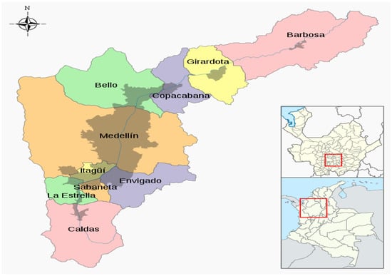
Figure 1.
Map of Valle de Aburrá.
Considering the characteristics mentioned above, Valle de Aburrá is a perfect case study for predicting PM concentrations [2]. Due to its topographical location, it experiences dry and rainy seasons. However, the main climatic phenomenon occurs during the transition between seasons, when a layer of low-altitude clouds covers the valley and reduces atmospheric turbulence, causing an increase in the concentration of polluting gases and particles produced inside the valley. These events are declared as critical air pollution episodes, and their occurrence has become an environmental risk factor that authorities and citizens are seriously concerned about.
Figure 2 shows the elevation map of Valle de Aburrá. The elevation has a minimum value of 1300 m and a maximum of 2800 m, as previously mentioned. This map makes it possible to analyze and support the phenomenon of thermal inversion because it shows how Valle de Aburrá is located at a height of approximately between 1500 m and 1000 m meters above sea level and its surroundings constitute a height of approximately between 2300 m and 2900 m above sea level, generating a kind of mountainous “wall” around Valle de Aburrá. This wall favors the phenomenon of thermal inversion since it makes the flow of air currents within the Valle de Aburrá difficult, increasing atmospheric pressure when it rains and generating an increase in relative humidity.
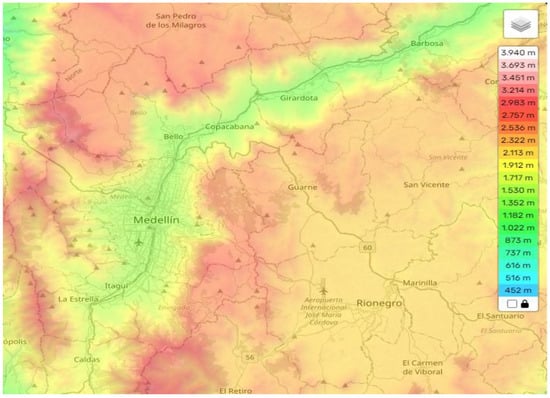
Figure 2.
Elevation map of Valle de Aburrá.
2.2. Data Analysis
This section presents the methods and techniques that were implemented to analyze PM2.5 data in Valle de Aburrá. First, we describe the sources we used to obtain such data and how we collected and processed them. Then, we perform a graphical analysis to better understand the behavior of the different variables that were considered in this study.
2.2.1. Air Quality Data
Valle de Aburrá extends from the municipality of Caldas in the south to the municipality of Barbosa in the north. There are around 36 air quality monitoring stations and 48 meteorological stations spread across its ten municipalities. Such stations include humidity and temperature sensors (thermo-hygrometers), pressure sensors (barometers), radiation sensors (pyrometers), and PM10 and PM2.5 sensors. These stations are managed by the SIATA, which is responsible for storing and analyzing the collected data. Since SIATA is a public entity, users are free to download and use such data [14].
For the purposes of this study, data on humidity, temperature, pressure, wind speed, and PM2.5 concentrations were downloaded. To evaluate the behavior of PM concentrations in Valle de Aburrá in particular, we downloaded the data captured by air quality station 48 and meteorological station 332 throughout 2019 and consolidated them into one dataset. This dataset was used to graphically analyze the behavior of the variables in the different areas of Valle de Aburrá and during the various seasons, as well as to identify models and train the neural network. Additionally, we downloaded the data captured by the northern (stations 73 and 82), southern (stations 229 and 78), and central (stations 68 and 12) air quality monitoring stations throughout 2018. This dataset was used to validate the performance of the techniques and the obtained results.
Figure 3 shows the location of the air quality monitoring stations throughout the Aburrá Valley (blue dots) and a real system for monitoring air quality and meteorological variables.
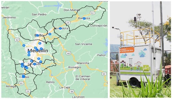
Figure 3.
Location of PM2.5 concentration monitoring stations around Valle de Aburrá [15].
In conclusion, we used two data sets: (i) one that contained data captured in 2019 from three meteorological and air quality stations and (ii) another that contained data captured in January, April, and June 2018 by three monitoring points along Valle de Aburrá. The resolution of the data or sampling time of the sensors are 1 h for each variable, this resolution is defined and limited by the SIATA database.
2.2.2. Graphical Analysis
The first dataset, which contained information for 2019, was employed to conduct a graphical analysis and examine two main aspects of the behavior of the meteorological variables and PM2.5 concentrations. The first aspect to be assessed was the relationship between the dynamics of the meteorological variables (humidity, temperature, pressure, and wind speed) and PM2.5 concentrations. By means of such analysis, it is possible to correlate the increase and decrease in PM2.5 concentrations with the increase and decrease in each meteorological variable.
The second aspect to be evaluated was the behavior of PM2.5 concentrations during the different seasons. For such purpose, the first database was divided into four seasons. As stated in [16], Valle de Aburrá experiences four distinct seasons during the year: (i) a first dry season, which begins during the last 15 days of December and ends during the first 15 days of March; (ii) a first rainy season, which begins during the last 15 days of March and ends during the first 15 days of May; (iii) a second dry season, which begins during the last 15 days of May and ends during the first 15 days of September; (iv) a second rainy season, which begins during the last 15 days of September and ends during the first 15 days of December.
Although this graphical analysis seeks to examine the behavior of the variables during the four seasons, the primary purpose of this study is to determine whether their behavior varies enough to identify a model and a neural network for each season.
2.3. Identification and Prediction of PM2.5 Dynamics
This section describes the process for the identification of a state-space model of PM2.5 dynamics to replicate the behavior of the variables and design state estimators. This section also illustrates the structure of the Kalman filter (state estimator), which can filter and predict unmeasurable or unknown variables. Once implemented, this estimator is called a virtual sensor.
2.3.1. Model Identification
State-space models mathematically express physical systems as series of input, output, and state variables linked by differential equations of any order in the time domain. These differential equations are combined in first-order matrix differential equations. The variables are represented as vectors and, when the dynamic system is linear and time-invariant, the algebraic equations are written as matrices [17].
In this case, we sought to identify a state-space model to obtain a mathematical expression in matrix form that predicted the behavior of PM2.5. The model was developed from the data because there were no phenomenological models based on differential equations validated in Valle de Aburrá. Different methods for the identification of dynamical systems with representation in state-space have been reported in the literature [18,19]. Currently, there are tools made under specialized software that guarantee the effectiveness of the methods. In this case, the MATLAB System Identification Toolbox was used. Therefore, we generated a system transfer function and labeled as input variables the humidity, temperature, pressure, wind speed, and PM2.5 data of 2019. Laplace transform generated a matrix relationship between each of the variables and the selected output, which, in this case, was PM2.5 data, delivering a discrete-time state-space system. The mathematical structure of a state-space system is as follows:
where is the system state vector, represents the input vector, denotes the output vector, is the discrete state matrix, represents the discrete input matrix, and is the discrete output vector.
2.3.2. State Estimator
State estimation is a branch of control theory that comprises different mathematical tools that can provide real-time information on difficult-to-measure variables using a dynamic model of the system and an available measurement of the real plant. State estimation is generally used in monitoring and control tasks of dynamic systems because it can predict, filter, and smooth unmeasurable or unknown signals and close control loops. When a state estimator is implemented in a real application as a predictor, it is called a model-based virtual sensor and serves to provide unavailable information and reduce the number of physical sensors in a given process, thus, reducing costs.
In this specific case, we employed a Kalman filter, which is an algorithm introduced by Rudolf E. Kálmán and used in control loops [20]. This, along with the concept of observability, is one of the most relevant developments by the researcher. The Kalman filter consists of two stages, prediction and correction, which can be described using a discrete linear system, as shown below:
The prediction stage consists of calculating the current state of the variables (Equation (5)) and the error covariance (Equation (6)) based on the error covariance at the previous instant. Here, represents the system state vector, denotes the input vector, is the output vector, and is the discrete-time state matrix. Therefore, = (I − A), = B represents the discrete-time input matrix and = C represents the discrete-time output vector.
In the correction stage, the Kalman gain (Equation (7)) is updated using the error covariance calculated in the prediction stage. In addition, measurements are taken, and the state estimate (Equation (8)) calculated in the prediction stage is corrected. Finally, the error covariance is updated (Equation (9)) using the Kalman gain and the error covariance calculated at the previous instant. The Q and R parameters of the Kalman filter are used to tune it. Q represents the model uncertainty, while R denotes the measurement uncertainty.
The stages and equations described above constitute the basic and general structure of the Kalman filter. However, due to its easy implementation and robustness, this algorithm has many variants, such as the extended Kalman filter and the unscented Kalman filter, as well as others that vary in some calculations, but they always maintain the described structure [21]. This is the basis on which the linear Kalman filter was developed.
2.3.3. Performance Indicators
Performance indicators are mathematical tools or algorithms that quantitatively evaluate the operation and performance of the estimators, considering the execution times and the accumulated error because they depend on the data and their performance is random [22]. Below are some performance indicators typically used to assess the performance of state estimators.
- I.
- Integral of the Time-Weighted Absolute Error
The integral of the time-weighted absolute error (ITAE) is a performance index weighted by time; therefore, it does not penalize the initial errors but those accumulated during the execution time. This indicator is obtained using the following mathematical expression:
where is the time vector of the system and is the estimation error.
- II.
- Integral of Absolute Error
The integral of absolute error (IAE) is an index that identifies the average variability of the response curve. In other words, it can measure the deviation of the process variables. The IAE is obtained by the following equation:
where corresponds to the absolute value of the estimation error and is the time vector of the system.
- III.
- Integral of Squared Error
The integral of squared error (ISE) can measure the deviation of the process variables and weigh the largest errors during the execution time. The following equation is employed to obtain this index:
where is the square of the estimation error and is the time vector of the system.
3. Results and Discussion
This section sequentially describes the development of a virtual sensor for PM2.5 prediction. It consists of five subsections:
3.1. Analysis and Correlation of Variables
We graphically analyzed the meteorological variables and the PM to establish a relationship between their dynamics. To this end, we plotted the behavior of each variable for 48 h.
Figure 4 compares PM (µg/m3), humidity (percentage %), and temperature (Degrees Celsius °C). This chart shows that PM has a directly proportional relationship with humidity and an indirectly proportional relationship with temperature. That is, when the environment humidity is higher, there is greater PM concentration; similarly, when the temperature is higher, there is lower PM concentration. The unit of measurement used for particulate matter is micrograms per cubic meter (µg/m3).
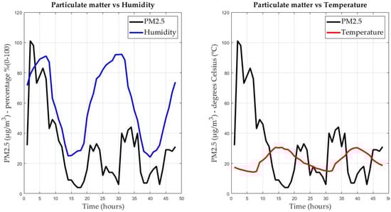
Figure 4.
Relationship between particulate matter, humidity, and temperature.
Figure 5 compares PM, pressure (hectopascals hPa), and wind speed (meters per second m/s). This chart shows that PM has a directly proportional relationship with pressure and an indirect relationship with wind speed. From the previous analysis, we can conclude that two variables increase PM concentration, while two variables decrease it.
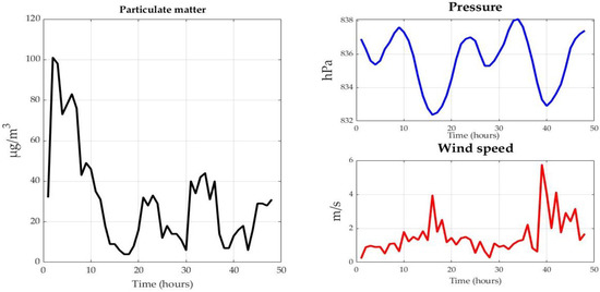
Figure 5.
Relationship between particulate matter, pressure, and wind speed.
Subsequently, we carried out an additional graphical analysis to observe the behavior of the meteorological variables (humidity, temperature, pressure, and wind speed) and the pollutants during the different seasons in Valle de Aburrá. The purpose of this analysis was to verify the variability in the minimum variables according to climatic changes because, as seen in the previous analysis, the dynamics of PM concentration may change depending on the behavior of some meteorological variables, which are subject to climatic changes. In addition, this analysis served to define whether a state-space model and a neural network could be developed for all seasons.
Figure 6 shows the PM dynamics in a one-week sample for each season. PM concentrations increased during rainy seasons 1 and 2 (red and green lines, respectively); however, no relevant differences were observed with respect to the dry seasons.
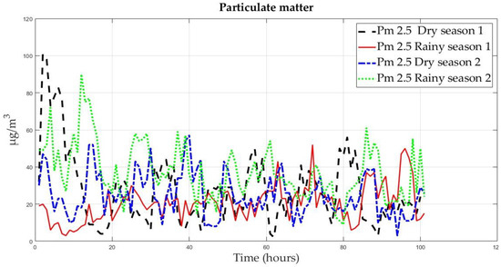
Figure 6.
Particulate matter dynamics in different seasons.
Figure 7 shows the humidity and temperature dynamics in the different seasons. Considering that Valle de Aburrá is located in the tropics, these variables do not present very varying dynamics.
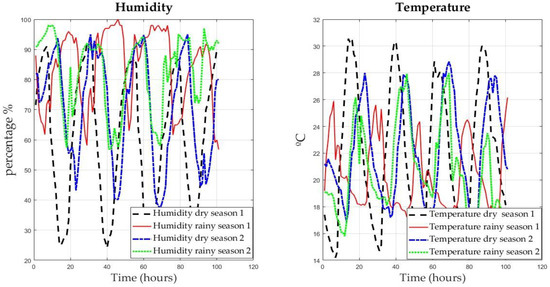
Figure 7.
Dynamics of humidity and temperature during the climatic seasons.
Figure 8 shows the pressure and wind speed dynamics in the different seasons. Note that, during the dry seasons, pressure decreases more than the other meteorological variables. Conversely, wind speed is more stable over the different seasons.
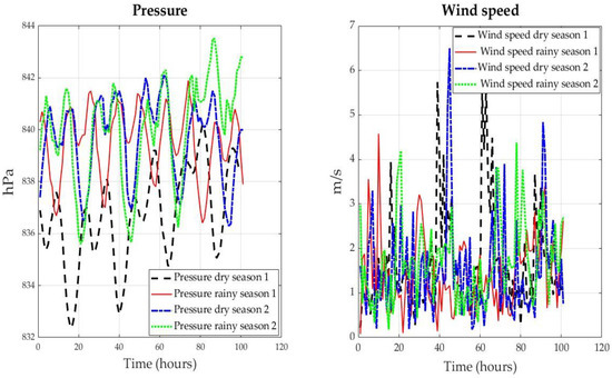
Figure 8.
Pressure and wind speed dynamics in different seasons.
3.2. PM Prediction Models
This section presents the models identified for the prediction of the PM2.5 concentration dynamics. Firstly, it introduces a prediction model based on a neural network. Subsequently, it describes the state-space model identified using the MATLAB System Identification Toolbox.
3.2.1. State-Space Model (Model SS)
Based on the 2019 data, we identified a state-space model to implement virtual sensors. The identification process started with the selection of the system inputs, meteorological variables, outputs (PM), and sampling times. Using the data and the Laplace transform, the toolbox generated a transfer function and the state matrices, respectively.
As shown in Figure 9, we identified three models to rule out the variables that added noise to the selection of the prediction model. The first model had four input variables, that is, the four meteorological variables; the second model had three input variables because wind speed was ruled out; the third model had two input variables, humidity and temperature. The subfigure on the left shows that the models with four and three input variables oscillated at the beginning of the forecast, which may be due to some of the meteorological variables contributing noise to the system. The subfigure on the right shows an extension of the previous description: the two-input model had much less oscillation and converged better to the real data. Therefore, the state-space model we implemented is the two-input model.
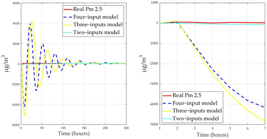
Figure 9.
Comparison of the identified models.
3.2.2. Kalman Filter
Considering that the two-input model is the one that best fits the data, the linear state-space system was rewritten using the following equations:
The dimension of the Ad matrix is 3 × 3, where humidity, temperature, and PM are related. The dimension of the Bd matrix is 3 × 2, where humidity and temperature are related. Lastly, the dimension of the Cd matrix is 1 × 3, where the measured variable is related. The values of the R and Q matrices were selected based on the algorithm’s performance. In other words, as the prediction improved, the values were increased until achieving the best result.
Equations (5)–(9) present the implementation of the Kalman Filter. Figure 10 shows that this filter (blue line) reduced the overshoot amplitude at the beginning of the prediction. In addition, its prediction was closer to the real data.
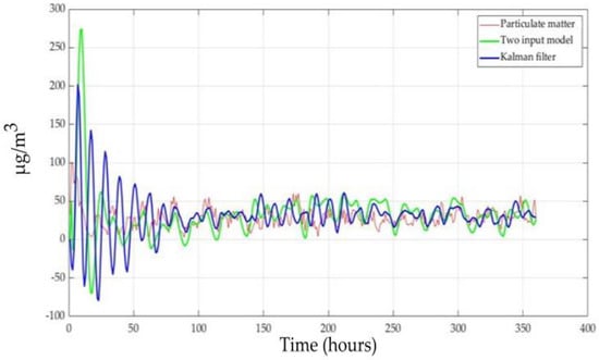
Figure 10.
Kalman filter prediction vs. model prediction.
3.3. Validation
The techniques were validated using the 2018 dataset to subject the system to unknown data. This dataset contains data captured in January, April, and June 2018 in the north, south, and center of Valle de Aburrá. The data were first filtered or smoothed because they contained measurement noise. Said filtering was carried out using the moving-window method, which takes a window of data from the dataset, calculates the average value of that window, and moves forward repeating the process, thus, removing invalid data and noise. The result of the data filtering is shown in Figure 11. The same procedure was replicated for the entire 2018 dataset.
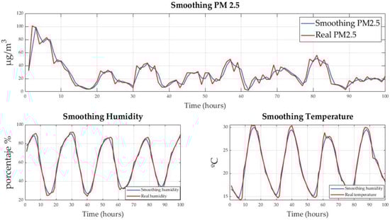
Figure 11.
Dynamics of smoothed variables.
Figure 12 shows the validation of the state-space model and the Kalman filter in the north of Valle de Aburrá for 15 days. This chart shows that the behavior of the model and the filter were similar to that of PM. Moreover, the filter corrected some sections of the simulation, significantly reducing the overshoot generated by the state-space model at the beginning.
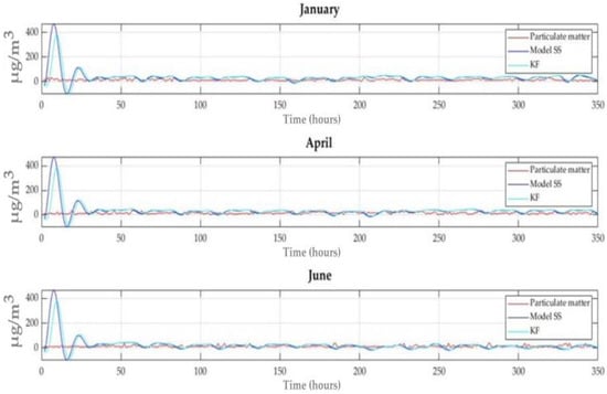
Figure 12.
Validation of the model and the filter in the north of Valle de Aburrá.
Figure 13 shows the validation of the state-space model and the Kalman filter in the south of Valle de Aburrá. Note that the prediction dynamics of the two techniques are consistent with those observed in the north. This overshoot or increase in the first 25 h is because the validation data is unknown to the system, so the prediction system (ss model and Kalman filter) takes about a day to adapt.
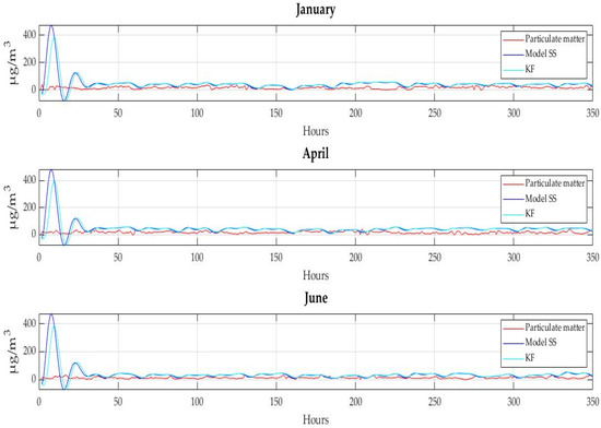
Figure 13.
Validation of the model and the filter in the south of Valle de Aburrá.
Figure 14 shows the validation of the state-space model and the Kalman filter in the center of Valle de Aburrá. This figure reveals abnormal behavior of PM in January, which may be due to sensor mismatch. The relevance of the filter and the model is then demonstrated because they accurately predicted the dynamics of PM, providing approximate information of better quality than that provided by the sensor at those instants of time.
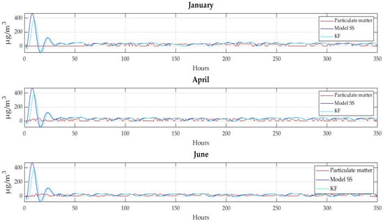
Figure 14.
Validation of the model and the filter in the center of Valle de Aburrá.
3.4. Performance Analysis
Table 1 presents the performance indicators in the north of Valle de Aburrá by validation month. Based on the ISE, we can say that there is variability between the estimator and the real data when big changes occur in the data. According to the ITAE, we can conclude that, although there is variability, the error accumulated during the estimator’s trajectory is not very significant, suggesting a reasonable estimation. The above is in agreement with the result of the IAE, whose low values demonstrate that there is little variability in the error along the trajectory.

Table 1.
Performance indicators in the north of Valle de Aburrá.
Table 2 presents the performance indicators in the south of Valle de Aburrá by validation month. In this case, the ISE, ITAE, and IAE are lower than those observed in the north, revealing better performance of the estimator and, therefore, better predictions. This may be related to the phenomenon; that is, the variables may have less variability or peaks, which would improve data acquisition and estimation.
Table 2.
Performance indicators in the south of Valle de Aburrá.
Table 3 presents the performance indicators in the center of Valle de Aburrá by validation month. In this case, the ISE, ITAE, and IAE values are higher than those obtained in the north and the south.
Table 3.
Performance indicators in the center of Valle de Aburrá.
4. Conclusions and Future Work
4.1. Conclusions
By comparing and segmenting the data, we found that the humidity and pressure variables have a directly proportional relationship with the increase in PM, while temperature and wind speed are inversely proportional. It is clarified that the results obtained are only validated in the context of Valle de Aburrá. Other locations may have different correlations due to their topographic and atmospheric conditions. In addition, we identified no significant differences among the variables throughout the different seasons of the year. Therefore, a PM behavior model can be adjusted for any season.
The behavior of the neural network and the state-space model are very similar. However, the neural network is not suitable for the design of virtual sensors. Conversely, the state-space model supports the development of Kalman filter-type virtual sensors to predict PM data.
The Kalman filter filters and predicts the dynamics of the state-space model; however, it has some tuning and sensitivity problems when it comes to predicting real PM2.5 data accurately. Furthermore, the Kalman filter can only follow the model data, maybe because the model has a deviation from the real data.
Assuming that this is the first state-space model for predicting contamination in Colombia, we can say that this is a first step towards a more robust PM prediction and diagnosis system.
4.2. Future Work
The actual implementation of the proposed algorithm is subject to permissions to acquire real-time data from SIATA. In this sense, as future work, it is expected to negotiate with the government entity the said permits for the next stage of this project.
Additionally, to achieve a better convergence in the prediction of the model and the virtual sensor, it is expected to explore two research routes. First, to obtain phenomenon-based model structures and identify parameters by means of artificial intelligence tools, and second, to implement more robust state estimation techniques, such as the particle filter [23] or moving horizon estimators (MHE) [24].
On the other hand, since the SIATA platform acquires measurements from sensors with different sampling times and measurements analyzed in the laboratory (offline measurements), another novel research route to explore are state estimation strategies that include asynchronous or non-uniform measurements [21]. Among them is the moving horizon estimator proposed by [25], where the information from offline sensors is used to update the initial conditions of the virtual sensor in each observation window.
Author Contributions
Conceptualization, M.L.G., E.R.A. and J.A.I.; methodology, C.M.H., M.L.G., E.R.A. and J.A.I.; formal analysis, C.M.H. and J.A.I.; software, C.M.H.; data curation, C.M.H. and M.L.G.; writing—original draft preparation, C.M.H.; writing—review and editing, C.M.H., M.L.G., E.R.A. and J.A.I.; visualization, C.M.H. and J.A.I. All authors have read and agreed to the published version of the manuscript.
Funding
This study was supported by the Instituto Tecnológico Metropolitano de Medellín within the framework of project P20220: “Sistema de monitoreo continuo y de predicción de la calidad del aire en Medellín a través de sensores virtuales para mejorar la estimación en línea de las variables ante incertidumbre paramétrica”.
Institutional Review Board Statement
Not applicable.
Informed Consent Statement
Not applicable.
Data Availability Statement
The data presented in this study are available from the corresponding author on reasonable request.
Conflicts of Interest
The authors declare no conflict of interest.
References
- Cardona, E.M. El área Metropolitana del Valle de Aburrá y las Provincias. Retos de unión social y política. Reflexión Política 2019, 21, 175–189. [Google Scholar] [CrossRef]
- Universidad Eafit. Informe Anual de Calidad del Aire 2021; Universidad Eafit: Medellín, Colombia, 2021. Available online: https://www.metropol.gov.co/ambiental/calidad-del-aire/informes_red_calidaddeaire/Informe-Anual-Aire-2021.pdf (accessed on 15 November 2022).
- Franco, J.F.; Gidhagen, L.; Morales, R.; Behrentz, E. Towards a better understanding of urban air quality management capabilities in Latin America. Environ. Sci. Policy 2019, 102, 43–53. [Google Scholar] [CrossRef]
- Karavas, Z.; Karayannis, V.; Moustakas, K. Comparative study of air quality indices in the European Union towards adopting a common air quality index. Energy Environ. 2020, 32, 959–980. [Google Scholar] [CrossRef]
- Gillen, B.; Snowberg, E.; Yariv, L. Experimenting with Measurement Error: Techniques with Applications to the Caltech Cohort Study. J. Politi-Econ. 2019, 127, 1826–1863. [Google Scholar] [CrossRef]
- Hime, N.J.; Marks, G.B.; Cowie, C.T. A Comparison of the Health Effects of Ambient Particulate Matter Air Pollution from Five Emission Sources. Int. J. Environ. Res. Public Health 2018, 15, 1206. [Google Scholar] [CrossRef] [PubMed]
- Al-Janabi, S.; Mohammad, M.; Al-Sultan, A. A new method for prediction of air pollution based on intelligent computation. Soft Comput. 2020, 24, 661–680. [Google Scholar] [CrossRef]
- Gogikar, P.; Tyagi, B.; Gorai, A.K. Seasonal prediction of particulate matter over the steel city of India using neural network models. Model. Earth Syst. Environ. 2019, 5, 227–243. [Google Scholar] [CrossRef]
- KGu, K.; Qiao, J.; Li, X. Highly Efficient Picture-Based Prediction of PM2.5 Concentration. IEEE Trans. Ind. Electron. 2018, 66, 3176–3184. [Google Scholar] [CrossRef]
- Yuchi, W.; Gombojav, E.; Boldbaatar, B.; Galsuren, J.; Enkhmaa, S.; Beejin, B.; Naidan, G.; Ochir, C.; Legtseg, B.; Byambaa, T.; et al. Evaluation of random forest regression and multiple linear regression for predicting indoor fine particulate matter concentrations in a highly polluted city. Environ. Pollut. 2019, 245, 746–753. [Google Scholar] [CrossRef] [PubMed]
- Jiang, H.; Wang, X.; Sun, C. Predicting PM2.5 in the Northeast China Heavy Industrial Zone: A Semi-Supervised Learning with Spatiotemporal Features. Atmosphere 2022, 13, 1744. [Google Scholar] [CrossRef]
- Nidzgorska-Lencewicz, J.; Czarnecka, M. Thermal Inversion and Particulate Matter Concentration in Wrocław in Winter Season. Atmosphere 2020, 11, 1351. [Google Scholar] [CrossRef]
- Yin, P.-Y.; Chang, R.-I.; Day, R.-F.; Lin, Y.-C.; Hu, C.-Y. Improving PM2.5 Concentration Forecast with the Identification of Temperature Inversion. Appl. Sci. 2021, 12, 71. [Google Scholar] [CrossRef]
- San Miguel, G.B. Lecciones Aprendidas Proyecto: Sistema de Alertas Tempranas de Medellin y el Valle de Aburrá-SIATA; Universidad Eafit: Antioquia, Colombia, 2016.
- Sistema de Alerta Temprana de Medellin, “SIATA.”. Available online: https://siata.gov.co/sitio_web/application/assets/img/contenido/Galeria/img_galeria_24.png (accessed on 15 November 2022).
- Alcaldía de Medellín. Plan de Acción Climatica Medellin 2020–2050; Alcaldía de Medellín: Medellín, Colombia, 2021. Available online: https://www.medellin.gov.co/es/wp-content/uploads/2021/09/PAC-MED_20210223.pdf (accessed on 15 November 2022).
- Alvarez, H.; Lamanna, R.; Vega, P.; Revollar, S. Metodología para la Obtención de Modelos Semifísicos de Base Fenomenológica Aplicada a una Sulfitadora de Jugo de Caña de Azúcar. Rev. Iberoam. Automática Inf. Ind. RIAI 2009, 6, 10–20. [Google Scholar] [CrossRef]
- Verhaegen, M. Filtering and System Identification: A Least Squares Approach; Cambridge University Press: Cambridge, UK, 2007; Volume 1. [Google Scholar]
- Ljung, L. Perspectives on system identification. Annu. Rev. Control. 2010, 34, 1–12. [Google Scholar] [CrossRef]
- Kalman, R. On the general theory of control systems. IRE Trans. Autom. Control. 1959, 4, 110. [Google Scholar] [CrossRef]
- Isaza, J.A.; Botero, H.A.; Alvarez, H. State Estimation Using Non-uniform and Delayed Information: A Review. Int. J. Autom. Comput. 2018, 15, 125–141. [Google Scholar] [CrossRef]
- Li, X.R.; Zhao, Z. Measures of Performance for Evaluation of Estimators and Filters. In Proceedings of the Signal and Data Processing of Small Targets 2001, San Diego, CA, USA, 26 November 2001. [Google Scholar] [CrossRef]
- Patwardhan, S.C.; Narasimhan, S.; Jagadeesan, P.; Gopaluni, B.; Shah, S.L. Nonlinear Bayesian state estimation: A review of recent developments. Control Eng. Pract. 2012, 20, 933–953. [Google Scholar] [CrossRef]
- Allan, D.A.; Rawlings, J.B. Moving Horizon Estimation. In Handbook of Model Predictive Control; Springer: Berlin/Heidelberg, Germany, 2019; pp. 99–124. [Google Scholar] [CrossRef]
- Isaza-Hurtado, J.; Botero-Castro, H.; Alvarez, H. Robust estimation for LPV systems in the presence of non-uniform measurements. Automatica 2020, 115, 108901. [Google Scholar] [CrossRef]
Disclaimer/Publisher’s Note: The statements, opinions and data contained in all publications are solely those of the individual author(s) and contributor(s) and not of MDPI and/or the editor(s). MDPI and/or the editor(s) disclaim responsibility for any injury to people or property resulting from any ideas, methods, instructions or products referred to in the content. |
© 2023 by the authors. Licensee MDPI, Basel, Switzerland. This article is an open access article distributed under the terms and conditions of the Creative Commons Attribution (CC BY) license (https://creativecommons.org/licenses/by/4.0/).