Abstract
We develop a new model for urban wind corridors analysis and detection of urban wind ventilation potential based on concepts and principles of network theory. Our approach is based solely on data extracted from spatial urban features that are easily obtained from a 3D model of the city. Once the spatial features have been extracted, we embed them onto a graph topology. This allows us to use theories and techniques of network theory, and in particular graph theory. Utilizing such techniques, we perform end-to-end network flow analysis of the wind potential across the city and, in particular, estimate the locations, strengths, and paths of the wind corridors. To calibrate our model, we use a dataset generated by a meso-scale climate model and estimate the model parameters by projecting the wind vector field of the climate model onto a graph, thus providing a meaningful comparison of the two models under a new metric. We illustrate our modeling approach on the city of Singapore and explain how the results are useful for climate-informed urban design.
1. Introduction
Wind plays an important role in city climatology due to its relevance for urban ventilation and transport processes, such as heat and pollutant transport [1]. Thus, understanding how to design urban ventilation patterns in order to improve wind flow is one of the key strategies for achieving good air quality [2,3], Urban Heat Island (UHI) mitigation [4,5], and Outdoor Thermal Comfort (OTC) [6,7], especially in densely-built urban areas. Such a relationship was further established in the studies by [8,9], where an association between area-level urban air ventilation and human health and mortality was made. Another important aspect is the use of wind as a clear source of energy that can reduce environmental emissions and energy costs, see [10]. Improving wind flow within the urban environment can assist in harvesting more renewable energy and should therefore be encouraged. The general pattern of wind in the city tends to be lower than in the suburban or rural areas, as a result of the aerodynamic response of wind to the urban structural form or morphology [11]. Buildings dominate the morphology of the city and also exert the largest resistance on air mass, which consequently reduces its velocity and compromises its ability to ventilate the urban canyon [12]. In the past, a lot of research has identified which urban parameters could best represent this building–airflow interaction [13,14] and has used these parameters to map the likely wind paths across the city [15].
One of the parameters that is known to be the best indicator of surface roughness for urban flow is the Frontal Area Index (FAI). One of the earliest concepts for the calculation of FAI was introduced by Grimmond and Oke [16]. Over the years, researchers came up with ideas to improve FAI generation to represent the urban roughness more accurately. Instead of summing up the entire facade area of every building, Burian [17] modified the FAI algorithm by only considering the building facets that are seen from a particular wind direction and by excluding the areas that are blocked by the windward buildings. In Hong Kong, ref. [18] introduced a new method to compute the Frontal Area Density (FAD), which only takes into account the facade area for a specific height band. They then used this parameter to develop a high-resolution FAD map that depicts the surface roughness of urban Hong Kong and correlated their results with wind tunnel experiments. In [19], the authors developed a method to calculate the FAI of buildings, infrastructure, and trees using an airborne Light Detection And Ranging (LiDAR) technique. Recently, ref. [20] presented different methods of calculating the FAI and made some recommendations regarding the optimal grid size. FAI is often used to determine wind paths because it considers the direction of the wind approaching the building facade. The surface area facing a particular wind direction can be seen as the blockage that can interfere the wind flow. Ref. [5] built on those similar concepts and developed a Least Cost Path (LCP) based approach to estimate the wind propagation throughout the city of Hong Kong. Interest in LCP-based wind corridor analysis has been consistently increasing over the years due to its simplicity, which makes it ideal for a wider implementation and users [12]. In [21], the authors developed a method that combines remote sensing and urban morphology information to calculate the LCP and construct ventilation corridors. However, validation of this approach by comparing the results with measurement data or other climate models has remained scarce.
Aside from the LCP-based method, there are several alternative approaches that researchers have explored for wind corridor analysis. In [22], the authors proposed using circuit theory to analyze large-scale urban ventilation environments. They used notions of conductivity and voltage as an analog to wind resistance and potential. Additionally, in [23], the authors improved the method presented in [22] and introduced new features such as the “neighborhood normalized current mode”. While this concept is interesting, it is not clear at all if it reflects the actual reality of how wind behaves and operates in an urban environment.
1.1. Limitations and Gaps in Current Research
While all the aforementioned papers present interesting and useful ideas in the direction of estimating wind corridors, there still exist a few significant issues that need to be addressed. Here we list the most important ones:
- Black box models-most studies on urban ventilation use off-the-shelf software, such as GIS tools [12]. This approach, while simple, introduces some limitations. The most important one is the inability to control, change, or adapt the methods used by those tools. This leads to a single common approach that is used in many of the papers, thus repeating the same set of problems and limitations that the GIS tools provide.
- Lacking physics effects of wind propagation- closely related to the previous point, most research on this topic has concentrated solely on urban friction as the driver of wind flow. While urban friction is a major contributor to wind flow patterns, it is not the only one. For example, one could also consider the force introduced in the prevailing wind direction and incorporate this effect into the model, in addition to the static urban friction.
- No calibration and validation framework- while many studies on urban ventilation have been presented, they have not been properly validated against real-world data. While some papers claim to have validated their results, this validation is mostly qualitative, based on visual inspection, rather than a quantitative validation that is based on first principles. Clearly, this aspect is not a simple one, and careful attention should be given to this important aspect.
What is the goal?
Research on urban wind and its impact on the local climate had been carried out for decades; see [24] for an overview. However, while urban atmospheric research has made significant progress, the knowledge transfer and implementation of these research findings into real practice still remains a big challenge. Some attempts have been made to make those results more accessible to domain specific experts by developing a standalone decision support tool; see, for example, [25,26,27,28,29]. Still, complications arise from the fact that architects and planners are working with wide design requirements and constraints, while researchers are usually studying only specific aspects of urban flow and consider only limited variables, case studies, and time periods. Hence, despite those attempts, it is difficult to generalize these research findings and make them applicable to non-experts.
Another issue is the complex method used in urban climate research. The majority of these experimental studies were done by either observational or computational methods. However, both methods require significant resources, such as time and cost. Design projects are usually done within an iterative process in a tight and fast-paced timeline. Thus, it is difficult to adopt these two methods into the design process. Also, special training needs to be undertaken to run these experiments properly, which normally is not part of the basic training for architects and planners.
What is needed?
Models that are simple, intuitive, and quick would be more helpful and beneficial for practitioners. To achieve this, some researchers have explored the idea of using spatial urban features that can be easily extracted from available open source data, and then using concepts from graph-based analysis methods, such as the well-known Least Cost Path (LCP) to predict the path of wind flow across the city [30]. This graph-based approach has significant advantages over computational climate models in terms of time and computational cost because there is no need to run heavy and complex simulations. Such methods are also intuitive and simple to understand, making the communication of the results to policymakers and decision makers simpler. Hence, such methods could be easily adopted by non-climatologists, such as planners and architects, to make scientific-based urban planning decisions.
This paper aims to introduce, from first principles, an analysis of regional-scale wind corridor networks that is more rigorous and accurate than previously presented. The directional information of the wind path as well as the urban feature, which is often neglected in the existing models, is one of the key components that we add to our model. Towards the end of this paper, we also present a new method of model calibration and validation with a meso-scale climate simulation by converting the wind vector field into a graph to allow for a meaningful comparison with our model.
1.2. Contributions
- We develop a wind corridor analysis framework from first principles of network theory and, in particular, graph theory.
- We develop an algorithm to estimate the connectivity (or porosity) of the city and analyze the ability of wind to access different spatial locations.
- We introduce important concepts and performance metrics of network theory that are relevant to the analysis of wind corridors.
- Using concepts from statistical learning, we develop a calibration and validation framework for the wind corridor model by estimating model parameters via a new discrepancy metric that offers an intuitive and fair comparison of the urban features-based model with a meso-scale climate model.
- We study the impact of the spatial resolution of the analysis on the wind corridor analysis and the impact of the spatial resolution on computation time.
- We study the impact that inaccuracies in the dataset can have on the wind corridor analysis and show that our method is robust against such distortions.
- We perform detailed theoretical computational complexity as well as practical time-run analysis of the proposed algorithm.
The rest of the paper is organized as follows: in Section 2, we present the methodology for the wind corridor algorithm. In Section 3, we present a statistical method for calibrating our model against a real dataset. In Section 4, we present detailed computational analysis of our algorithm. In Section 5, we present simulation results that include the calibration results, the sensitivity and uncertainty analysis of our model, and illustration of our framework for “what-if” scenarios. Finally, the paper ends with conclusions in Section 6.
1.3. Mathematical Notations Used
We now introduce many of the notations we will use in the rest of the paper. The symbols and denote the non-negative real and strictly positive integer numbers, respectively. The notation denotes a normally distributed R.V. with mean and variance given by and , respectively. By , we denote the statistical expectation of the random variable x. The symbol is the Iverson bracket, defined as:
We denote a matrix with m rows and n columns by . The -th entry of is denoted .
Definition 1
(Sub-matrix). Let have m rows and n columns. Define , such that both are nonempty. We name these sets as , and assume that and . Then we define sub-matrix of via .
Remark 1.
We shall use a special case of Definition 1, where and .
2. Methodology: Urban Feature Extraction and Network Theory Model
In this section, we develop the methodology for our wind corridor analysis. We are interested in finding likely air flow corridors based on the premise that wind across a city follows the path of least resistance [5]. This logic corresponds to computing the LCP, which finds the path of least resistance across a cost trajectory from a source point (SP) to a destination point (DP). By defining multiple SPs and DPs, we can find pathways that represent routes with strong ventilation potential and a high degree of connectivity. These are called wind corridors. Since we are considering multiple SPs and DPs, we need to define a metric that quantifies the contribution of each spatial location to the overall ventilation potential. Once such metric is known as the betweenness centrality of the LCPs. The shortest path betweenness centrality is a well-known metric in graph theory and has many applications in network theory [31]. A graphical representation of our framework is depicted in Figure 1, where the left panel is the wind corridor model and the right panel depicts the calibration of the model, which is presented in Section 3. Our approach is based on the following four steps:
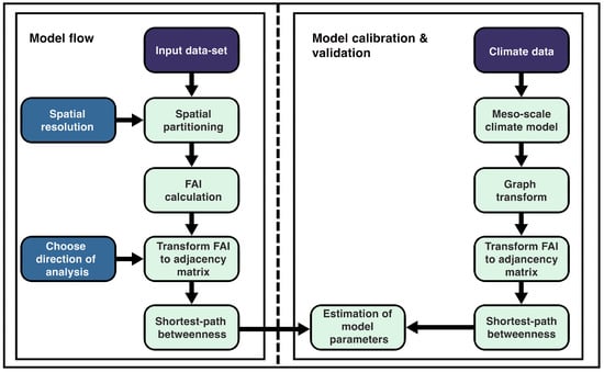
Figure 1.
System model. Left panel: the proposed framework where the input is the 3D dataset of building heights and the user needs to choose the spatial resolution and the direction of analysis. Right panel: the calibration of the proposed model against a meso-scale climate model.
- Morphology-based urban feature extraction: a digital topographic map is used to obtain the directional friction of the urban elements, which are used as spatial features.
- Network theory over graphs: using the information from the spatial features, we then model the urban topology as a weighted directional graph of a network flow.
- Shortest path analysis: using the graph structure, we calculate a multitude of source–destination shortest paths (in the sense of least resistance) in the direction of the prevailing wind.
- Calculation of betweenness centrality: given all the source–destination shortest paths, we calculate the centrality metric, known as the betweenness centrality, which can be interpreted as the wind corridors of the urban domain.
We now present details for each of the steps, which are also illustrated in Algorithm 1.
| Algorithm 1: Urban Wind Corridors Analysis via Network Theory |
Input: Buildings’ footprint dataset Required spatial resolution Direction of analysis Output: Shortest path betweenness matrix
|
2.1. Morphology-Based Urban Feature Extraction
In general, feature extraction refers to transforming the raw dataset into a much smaller dimension than the original dataset that can be processed, while preserving the information in the original dataset. In the context of our problem, the raw dataset is a 3D dataset that contains the buildings’ height information in high spatial resolution (e.g., 1 m). Our feature extraction procedure partitions the large dataset into smaller spatial cells and, for each cell, computes eight directional summary statistics that act as our urban morphology features. In particular, the feature we consider is known as the frontal area index (FAI) and is widely used in urban roughness parameterization [16]. We now present the details of how this feature is extracted from the dataset.
- Input dataset: given a 3D dataset that contains the buildings footprint (coverage) and respective heights inside the domain (e.g., Singapore), the dataset is represented by a matrix with rows, columns, and non-negative values (since the heights cannot be negative). Each entry in provides the height of the building at that spatial location (pixel) and is denoted by . In the case where a pixel does not contain a building, its value is zero.
- Spatial partitioning: the data matrix is partitioned into a set of non-overlapping sub-matrices; see Figure 2. We denote each matrix by , where the -th sub-matrix is obtained via Definition 1 as follows:where we define and This means that the spatial resolution of the dataset is finer than the grid’s.
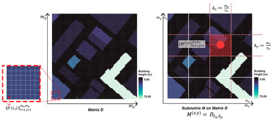 Figure 2. Left: Input dataset with spatial resolution of m. Right: Spatial partitioning into a set of matrices .
 - Total frontal area: the total frontal area (TFA) represents the area projected in the direction of the wind vector. We consider eight directions: , See Figure 3. A different number of directions can be obtained trivially, without any changes to the model. The TFA of the buildings in the -th cell at wind direction is given by the following two steps:
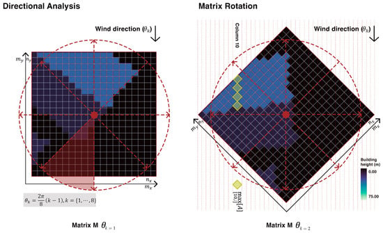 Figure 3. Left: Eight directions are considered; each covers 45 degrees of the plane. Right: Matrix rotation by degrees. Cells highlighted in yellow have the maximum value of this column. See Equation (4) for details.
- (a)
- Rotate matrix by degrees:where is the matrix rotation (projection) operator of matrix by degrees, where each -coordinate is rotated according to:and a new set of coordinates is obtained, .
- (b)
- Sum the maximum of each column of the rotated matrix (see Figure 4):
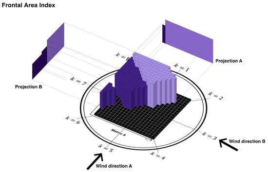 Figure 4. Projection of the maximum values into vertical 2D planes to calculate FAI in the direction .
where denotes the maximum value of the i-th column of matrix The matrix operation is described in other papers by , see [18]. - Frontal area index: the frontal area index (FAI) in direction can be written as a 3D matrix, where the coordinates indicate the spatial location and the k coordinate indicates the spatial direction:
Now that we have extracted the desired urban feature, that is, the FAI in each of the eight directions, we proceed with the analysis by modeling the urban ventilation via a graph.
2.2. Graph Theory over Network
Network theory provides the theoretical infrastructure for analyzing graphs and the flow of information in them. Informally, a graph is a structure that is formed with a set of vertices (or nodes) and a set of edges joining vertices that is used to model or represent a relationship [31]. Graphs are powerful data structures that provide the ability to express and represent various relationships (captured by the “edges”) between objects (represented by “nodes”). In the context of our problem, we model the vertices as a 2D grid, where each node represents a local, physical, spatial location. The edges represent the friction or the conductivity and connectivity among the different vertices. In particular, our setting is quite special in the sense that the resulting graph has a specific structure, known as the King’s graph [31]. This is due to the fact that each vertex has exactly eight neighbors, corresponding the the eight directions of spatial analysis.
Definition 2
(weighted directed graph [31]). A weighted directed graph , where is the set of N nodes (vertices), is the edge set, and is the weighted adjacency matrix with , if and zero otherwise.
In our model, we shall use a specific type of a graph structure called the King’s graph [31]. This type of graph arises in cases where the data are structured in a rectangular shape and each vertex has eight neighbors, arranged as a chess board. See Figure 5 for illustration.
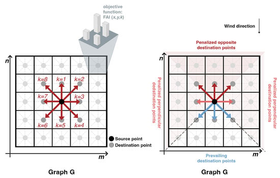
Figure 5.
Left: Representation of the King’s graph, with FAI as the cost of the edges. Right: Physics-inspired directional penalty weight matrix.
Definition 3
(King’s graph [31]). An King’s graph is a graph with vertices in which each vertex represents a square on an chessboard, and each edge corresponds to a legal move by a king. The King’s graph can be constructed by a strong product of two path graphs.
The cost of the edges is calculated based on the FAI . This requires us to translate the FAI values from the 3D structure into the 2D weight matrix . Noting that our graph structure is the King’s graph, the following result shows how this transformation can be obtained.
Definition 4
(Transforming FAI values to the weighted adjacency matrix ). The weight of an edge, is given by:
where we define:
where:
The procedure presented so far does not take into account the fact that we analyze the wind corridors in accordance with a particular choice of prevailing wind direction. We would like to incorporate this aspect into our model in a way that reflects this fact. Therefore, we add two penalty terms for cases where the directional change is or more than the prevailing wind direction, presented next. The logic of those terms is as follows:
- Penalize flow directions that are perpendicular to the prevailing wind direction, and define this penalty as
- Penalize flow directions that are opposite to the prevailing wind direction, and define this penalty as
Those penalties are incorporated into the graph model via the following penalty matrix.
Definition 5
(Directional penalty weight matrix). We define the following penalty weight matrix, which corresponds to analysis direction :
2.3. Shortest Path Analysis
The shortest path in graphs is a well-known and widely used problem that appears in many areas of science [31]. Although a more suitable and intuitive name for the same problem is the Least Cost Path (LCP), the shortest path is more commonly used, and we shall use them interchangeably. Generally, the edges represent the cost of traversing that edge. Depending on the application, the cost may be measured in time, money, physical distance (length), etc. The total cost of a path is the sum of the costs of all edges in that path, and the minimum cost path between two nodes is the path with the lowest total cost between those nodes. In our problem, the edges represent the friction of the connectivity path from one vertex to its neighbor, thus representing the “difficulty” of the wind passing through this edge. We now express the overall cost of a path that is composed of two components:
- The friction captured by the FAI as calculated in Section 2.1 and defined in Definition 4.
- The preservation of momentum as defined in Definition 5.
Definition 6
(Cost of graph paths). A path from a node to node in is made of a sequence of edges , and is denoted by . The total cost of the a path is a the sum of a function of the weights of the edges:
where .
Next we define the shortest path, which involves finding a path between two vertices (or nodes) in a graph such that the sum of the weights of its constituent edges is minimized.
Definition 7
(Shortest path on a graph). The shortest path from in is any path , such that:
where denotes the set of all paths between s and d.
Remark 2.
The optimization problem in Definition 7 can be formulated as a linear programming method and solved using dynamic programming methods, such as Dijkstra’s algorithm [32], the Bellman–-Ford algorithm [33], the algorithm [34], and others.
2.4. Setting the Source and Destination Sets for the LCP
To complete the specification of the LCP analysis, the sets of source points and destination points need to be determined. These sets depend on the direction of analysis, such that the set of source points is located along the boundaries of the domain that is aligned with the direction . The set of destination points is located also along the boundaries of the domain, aligned with direction , but from the other side; see Figure 6 for illustration for the case .
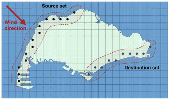
Figure 6.
The domain is the light green shape, partitioned into a King’s graph structure (black squares), denoted . The source (black dots) and destination (dark blue dots) sets are indicated for by the red arrow.
2.5. Calculation of Betweenness Centrality Metric
The concept of centrality is central for the analysis of networks. The notion of betweenness is one of the most prominent measures of centrality in networks, although many others also exist [30]. The concept of betweenness centrality is used as a measure of centrality in a graph, based on shortest paths [30]. For every pair of vertices in the graph, there exists at least one shortest path between the vertices. The betweenness centrality for each vertex is the number of these shortest paths that pass through the vertex. Simply put, betweenness centrality counts the fraction of shortest paths between a pair of nodes that an intermediate node lies on and sums these fractions over all node pairs that are defined a-priori.
Definition 8
(Shortest path betweenness [30]). Let be a set of starting points and be a set of destination points. Let be the number of shortest paths. Let be the number of shortest paths passing through some vertex other than . The (shortest path) betweenness, , of a vertex is defined to be:
where and are the length of the path. By , we denote the shortest path betweenness matrix, which represents how many shortest paths traverse through each node in the graph.
Remark 3.
We note that in Definition 8, the conventional shortest path betweenness uses , while the shortest path bounded distance betweenness uses .
3. Model Calibration and Validation Using Climate Model Data
The model that was developed in the previous section, while logical, needs to be tested against a real dataset in order to learn how accurately it reflects the urban wind flow under realistic conditions. The question that needs to be addressed is: How do we compare the results we obtain using the graph structure with climate data?
To this end, we need to be able to create a common ground for this comparison, and we propose to use the shortest path betweenness metric as the measure of discrepancy between the two. Therefore, we need to be able to translate a real-world dataset into the graph structure presented earlier and calculate the shortest path betweenness metric for it.
Clearly, the best way to perform such a comparison would be against real-world observations that have been collected from high-quality weather stations, densely deployed inside the domain. This scenario is not practical in most cases, since weather stations are usually sparsely deployed. For this reason, it would not be practical to use weather stations as the basis for a comparison to our model, since we will not be able to convert the data obtained from weather stations into a complete graph. Instead, what we can achieve practically is to compare our results with the best possible meso-climate model available. While climate models are less accurate than weather stations and introduce estimation errors, the process that we shall employ will significantly reduce these errors. This will be possible by averaging the climate model data over a long period of time, thus shrinking the uncertainty of the model output.
We now present a simple approach for transforming a spatio-temporal dataset that could be obtained by running a meso-scale climate model into a graph structure. This will serve as the baseline for achieving two goals: calibrating our algorithm and testing its agreement with our algorithm.
3.1. Deriving the Graph Weights from the Climate Model Wind Vector Field
We define the output of the climate model as a 3D matrix (spatio-temporal) index set, such that are the spatial 2D plane and is the time domain. Then we can express the vector of wind speed and direction in each cell as a vector:
In order to transform the climate model output to a graph structure, we need to map the wind speed and direction in each cell into eight weights, corresponding to the FAI values. To do that, we quantize the direction component into eight quasi-spaced bins, each covering 45, represented by , followed by time averaging, as follows:
where Now that the directional FAI values have been estimated, we can calculate the cost of the edges in the same manner as for the urban parameters. This is the basis for a meaningful comparison between the two models.
We note here that the inaccuracy of the climate model will not have a serious impact on the results because of the averaging over a long period of time T, which is the simulation length. The larger T is, the smaller the effect of the climate model errors would be.
3.2. Calibration of the Morphology-Based Model
We now explain and derive a rigorous algorithm to calibrate the morphology-based model. Recall that the three free model parameters are:
- The penalty term (see Definition 5).
- The penalty term (see Definition 5).
- The path length L (see Definition 8).
To obtain an optimal estimate of these values, we need to choose a sensible distance metric between the morphology-based model and the climate data-based model. While there are myriad choices, here we present a simple and common choice of distance metric.
Definition 9
( (Euclidean) distance). Given two matrices of the same dimensions, , the distance is defined as:
In the context of our problem, the two matrices are the shortest path betweenness matrices, one of the climate model and one of the urban morphology-based analysis.
3.3. The Calibration Process via Grid Search
In order to find the optimal set of parameters, we use the Least Squares (LS) optimization problem, where we consider eight directions of analysis and average over them the discrepancy between the two models’ output. We therefore obtain a set of eight shortest path betweenness matrices for each of the models, denoted by , and the LS optimization is given by:
where and .
A direct solution for this optimization problem is impossible, since it involves obtaining the derivatives with respect to of matrices , which themselves depend on the LCP algorithm used. Instead, a numerical solution is pursued. Since this optimization problem involves continuous decision variables , there are an infinite number of points in the domain, and complete enumeration is impossible. A common approach is to perform a grid search, essentially discretizing the domain. A grid search creates an equally spaced grid of points over the feasible region and evaluates the objective function at each point. Grid search is an exhaustive search method, so the required search time for obtaining the solution is deterministic and can be calculated. Since our problem is only three dimensional, this problem can be solved efficiently.
4. Theoretical Computational Complexity
In this section, we analyze the computational complexity of our algorithm from a theoretical perspective. This is very useful and helps us understand how the computational complexity of the algorithm scales with different choices of the model parameters, such as cell size.
Computational complexity represents the algorithm’s worst-case complexity. The Big O (denoted ) defines the run-time required to execute the algorithm as a function of the size of the input parameters and the number of steps it takes to complete; see [35] for details. Computational complexity measures how efficient an algorithm is for a large parameter space (asymptotic behavior), which means that this is a measure of the worst case [36]. To perform the analysis, we follow the steps presented in Algorithm 1 and analyze each individually:
- Feature extraction (Steps 2–12): The algorithm requires a nested triple loop that runs times. All operations are of with the exception of finding the maximum of unsorted array (Step 7), which has complexity. Therefore, the overall complexity of this step is .
- Graph theory over network (Steps 14–16): The algorithm requires a nested triple loop that runs times. All operations are of . Therefore, the overall complexity of this step is .
- Shortest path and betweenness centrality (Steps 17–22): The algorithm requires a nested loop with computational complexity of . The shortest path operation via the Dijkstra algorithm in Section 2.3 has a computational complexity of for a single source–destination [31]. For the King’s graph, we have and [31], and therefore we obtain that the computation complexity of the algorithm is
Combining all those elements we obtain that the computational complexity of the algorithm is given by
To complement the theoretical analysis, it is also important to provide practical analysis of the time complexity it takes to run the algorithm. This will be presented in the following section.
5. Simulation Results
In this section, we present detailed results regarding the performance of our methodology. The algorithm that we developed and is presented in Algorithm 1 was implemented in Python. As a real-world and practical example, we consider the analysis of wind corridors in Singapore. See Figure 6 for an illustration of the domain . The island of Singapore is located north of the Equator, between 109 N and 129 N, and 10336 E and 10425 E, at the southern tip of the Malaysian peninsula, and is considered tropical with a typical equatorial wet climate. The building information for our analysis was obtained from the publicly accessible open source platform Openstreetmap (https://www.openstreetmap.org, accessed on 1 February 2023).
This section is divided into the following parts:
- Model calibration using climate model spatio-temporal wind patterns.
- Practical algorithmic time complexity.
- Sensitivity analysis of the algorithm to the size of the cells.
- Uncertainty quantification analysis of the algorithm to errors in the urban morphology dataset.
- Illustration of how the algorithm can be used to analyze “what-if” scenarios by considering developments of new areas.
5.1. Calibration of the Model Using Meso-Scale Climate Model
We present the results of the calibration of our model using a meso-scale climate model. The climate model we use is the Multilayer Urban Canopy Model (MLUCM) embedded in Weather Research and Forecasting (WRF) version , which incorporates the Building Effect Parametrization (BEP) and the Building Energy Model (BEM) [37,38]. The details of the model set-up can be found in [39,40,41]. The spatial resolution of the WRF model is m. After estimating the model parameters in Equation (12), we found that the optimal parameters are . From the results of the experiment, it seems that, while there is a larger sensitivity of the quality of the fit to choices of , the sensitivity to the choice of L is quite low and may have negligible impact on the results. The results of the model calibration are depicted in Figure 7. The results show that, while the WRF model provides more detailed and nuanced information, the main characteristics are also found in the urban morphology-based approach. This means that our model can serve as a reasonable proxy for the computationally demanding climate model.
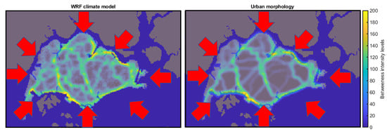
Figure 7.
Comparison of the network model (right panel) with the climate model (left panel). The results are based on the accumulation of all eight directions, .
5.2. Practical Algorithmic Time Complexity
The result we obtained in Equation (13) provides us with a bound on the asymptotic growth rates, that is, as . We are also interested in the non-asymptotic case. This requires running the algorithm for different configurations. One configuration that is of importance is the running time of the algorithm as a function of different cell sizes. To this end, we divide the analysis into two parts:
- Feature extraction.
- LCP analysis, where we consider four wind directions: NS, W–E, NE–SW and NW–SE.
We consider the cell size of . First, in Figure 8, we present the number of LCP pairs that need to be calculated for each cell size. This is important as it has a direct impact on the run-time of the algorithm, as we have shown in the computational complexity analysis earlier. Next, in Figure 9, we present the execution time as a function of cell size, where the algorithm was executed on an Intel(R) Core(TM) i7-8565U CPU@ GHz with 4 cores.
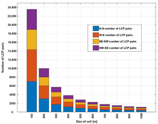
Figure 8.
Number of LCP pairs at four different spatial directions as a function of cell size, .
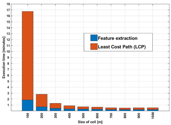
Figure 9.
Computational time in minutes as a function of cell size.
5.3. Sensitivity Analysis
We study the sensitivity to cell size; the question of interest is: does the choice of the size of the cell (i.e., ) have an impact on the results of the analysis, and to what extent? This question is also related to the computational complexity of the algorithm, as we saw in Section 4. We investigate the sensitivity to cell size by running the model for various values where, for simplicity, we set . In Figure 10, we present the N–S wind corridors for m. The results show that increasing the cell size reduces the level of detail. This makes sense, since the larger the cell size, the more we average the information in order to calculate the FAI values. One should interpret this result jointly with the computational time presented earlier and make an informed decision regarding the spatial resolution and time complexity trade-off that works best for their purposes.
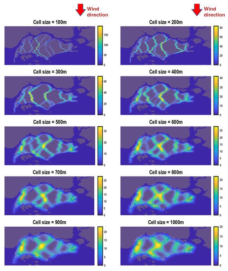
Figure 10.
North–south () wind corridors for different sizes of cells.
5.4. Uncertainty Quantification
We also studied the uncertainty quantification due to buildings’ height errors. The question of interest is: do errors (e.g., uncertainty) in the original 3D dataset have an impact on the results of the analysis, and to what extent? This question is of practical interest, since in many cases the dataset is obtained from open sources that may not be fully accurate. Generally speaking, uncertainty quantification (UQ) involves obtaining a set of randomly generated input values, passing them through our model, and obtaining the performance indices. To this end, we perform UQ of our algorithm, where we investigate the impact that variations in the input dataset have on the output of the model. This means that first we need to construct a model that represents how the uncertainty is manifested in the dataset, and how this uncertainty propagates to the performance index, defined as the shortest path betweenness matrix . We use the following model for generating samples from the dataset buildings’ heights:
where means the maximum of a and b; and denote the true (and unavailable) and the noisy (and available) urban morphology datasets, respectively. By , we denote the noise realization of each pixel. The max operation guarantees that the resulting process has no negative values, corresponding to negative heights. By increasing the values of , we consider a more “noisy” and less accurate dataset. When , we assume that the dataset is perfectly accurate, and that will serve as our benchmark.
Our goal is to compute the expectation of by averaging over all possible values of , which can be written as:
where is our model for calculating . Since a direct calculation of this quantity is impossible, we instead implement a Monte Carlo (MC) sampling procedure to approximate the above expression:
where N is the number of MC samples and is the n-th realization from the distribution presented in Equation (14). Samples from this density can be generated easily using a rejection mechanism from importance sampling [42]. The MC estimator is an unbiased estimator since the expected value of is equal to and, according to the strong law of large numbers, the average converges almost surely to the true expected value [42]. In Figure 11, we present the N–S wind corridors for m, where we vary the noise levels, , and set the number of MC samples, . The results show that, up to noise values of , the impact is quite small, and that for values larger than that, some of the details are lost. We further quantify this effect by comparing the distance between the noiseless case (e.g., ) with the other eight noisy scenarios. The results are depicted in Figure 12 and show an increase in the distance of the metric, which saturates at .
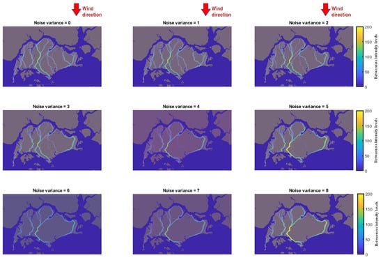
Figure 11.
Uncertainty quantification of the algorithm to noisy dataset , for spatial resolution m, under North–South () wind analysis.
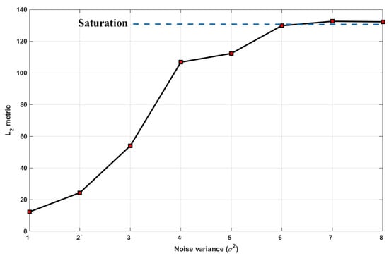
Figure 12.
Uncertainty quantification of the LCP algorithm to noisy dataset , measured via the metric in Definition 9, for spatial resolution m.
5.5. Wind Corridor Analysis for “What-If” Scenarios
To demonstrate how our model can be applied in the real world, we develop some “what-if” scenarios (WiS) for Singapore. We select large open spaces that are currently planned for future development, such as Paya Lebar Airbase District (PLAB) on the northeastern side of the island, and Tengah forest, located at the west side; see Figure 13. The buildings are copied from the existing district, namely the Central Business District (CBD), known as one of the densest built-up areas of the city. Next, we then increase the built-up areas in each of these districts. First, we take the baseline case and copy the CBD buildings onto the PLAB district only, and Tengah area only, in Scenarios 1 and 2, respectively. Lastly, for Scenario 3, we combine both Scenarios 1 and 2 so that the built-up density is high in both selected districts. These scenarios, however, were created solely for testing purposes, without any intention to be a sort of recommendation for future urban design and planning. Then, we cross-compare these WiS against the baseline scenario, which closely reflects the current state of the island.
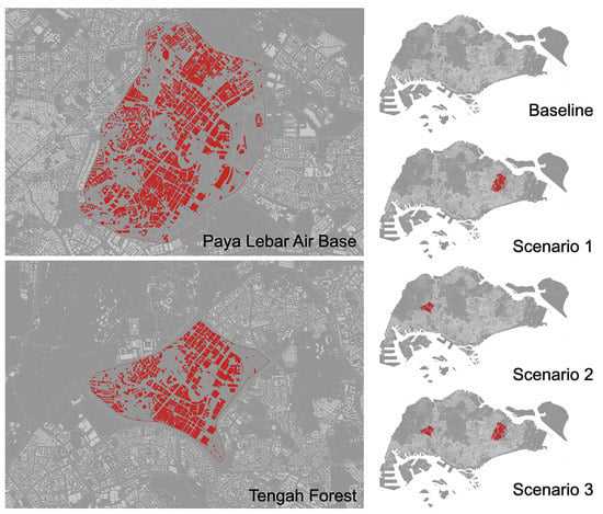
Figure 13.
Illustration of the “what-if” scenarios. The newly added built-ups were created only for testing purposes.
The results of this analysis are presented in Figure 14 and Figure 15, which show that the hypothetical developments can have a significant impact on existing wind corridors. Some wind corridors may be shifted, while some may be split into a collection of less intense ones. Those results show the benefit of our analysis and could have a significant impact on how decision makers and policymakers approach future planning of the city.
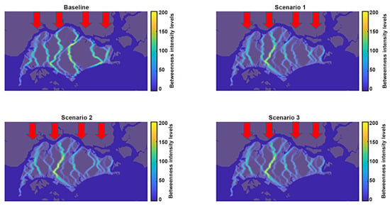
Figure 14.
“What-if” scenario: The prevailing wind is North–South, (), indicated by the red arrows.
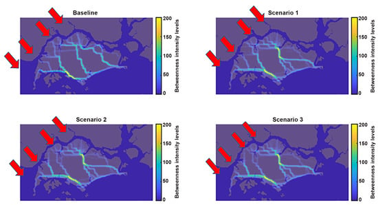
Figure 15.
“What-if” scenario: The prevailing wind is Northwest–Southeast, (), indicated by the red arrows.
5.6. Discussion and Insights
The goal of this paper was to develop a simple yet mathematically tractable framework to analyze wind corridors. We now summarize the main findings and make recommendations that could be useful for urban designers and policymakers.
- The proposed model is capable of achieving similar results as a meso-scale climate model under the proposed metric.
- The computational complexity of the proposed algorithm is on the order of minutes, while the same type of analysis would take days if not weeks via the numerical climate model.
- The model is robust to uncertainty in the input morphology data. This is important since, in many practical cases, only open source datasets are available and may contain inaccuracies and be noisy.
- Careful consideration should be given to the choice of the spatial resolution of the analysis: while high resolution results may be desirable, they come at the cost of a higher computational complexity burden. The user of the system should be regarding this trade-off and make the best decision for their purposes.
- We demonstrate how our framework could be used by urban planners to make informed decisions regarding how future design candidates may impact the wind flow inside the city. This may have a significant impact on how heat or pollution is removed from the city, contributing to the overall quality of life of the city’s residents.
- The algorithm we developed is suitable for any city around the world. It would be beneficial if more studies used this model and tested it on different configurations and different urban set-ups.
6. Conclusions
We presented a new model for urban wind corridor analysis and detection of urban wind ventilation potential. Our method is based on network theory and uses only data extracted from spatial urban features that can be easily obtained from a 3D model of the city. We performed end-to-end network flow analysis of the wind potential across the city and, in particular, estimated the locations, strengths, and paths of the wind corridors. We used a dataset generated by a meso-scale climate model to first estimate the model’s parameters and then validate the accuracy of our model by projecting the wind vector field of the climate model onto a graph, thus allowing for a meaningful comparison of the two models. We illustrated our modeling approach on the city of Singapore and explained how the results are useful for climate-informed urban design. Such designs are important as they help improve wind flow within the urban environment, which can improve thermal comfort as well as the harvesting of renewable energy. Future research directions include the incorporation of different urban features currently not considered by this model, such as ground elevation, trees, and water bodies. Further studies of the model in other cities around the world would increase and enhance its accuracy and usability.
Author Contributions
I.N.: conceptualization, methodology, software, validation, formal analysis, investigation, resources, data curation, writing—original draft, writing—review and editing, visualization. A.S.A.: conceptualization, methodology, software, validation, formal analysis, investigation, resources, data curation, writing—original draft, writing—review and editing, visualization. All authors have read and agreed to the published version of the manuscript.
Funding
This research was funded by the National Research Foundation (NRF) of Singapore under the Cooling Singapore project.
Institutional Review Board Statement
Not applicable.
Informed Consent Statement
Not applicable.
Data Availability Statement
Openstreetmap can be found here https://www.openstreetmap.org (accessed on 1 February 2023).
Acknowledgments
The research was conducted under the Cooling Singapore project, funded by Singapore’s National Research Foundation (NRF). Cooling Singapore is a collaborative project led by the Singapore–ETH Centre (SEC), with the Singapore–MIT Alliance for Research and Technology (SMART), TUMCREATE (established by the Technical University of Munich), the National University of Singapore (NUS), the Singapore Management University (SMU), and the Agency for Science, Technology, and Research (A*STAR).
Conflicts of Interest
The authors declare no conflict of interest.
References
- Fernando, H.J.; Zajic, D.; Di Sabatino, S.; Dimitrova, R.; Hedquist, B.; Dallman, A. Flow, turbulence, and pollutant dispersion in urban atmospheres. Phys. Fluids 2010, 22, 51301. [Google Scholar] [CrossRef]
- Buccolieri, R.; Sandberg, M.; Di Sabatino, S. City breathability and its link to pollutant concentration distribution within urban-like geometries. Atmos. Environ. 2010, 44, 1894–1903. [Google Scholar] [CrossRef]
- Yang, J.; Shi, B.; Shi, Y.; Marvin, S.; Zheng, Y.; Xia, G. Air pollution dispersal in high density urban areas: Research on the triadic relation of wind, air pollution, and urban form. Sustain. Cities Soc. 2020, 54, 101941. [Google Scholar] [CrossRef]
- Hsieh, C.M.; Huang, H.C. Mitigating urban heat islands: A method to identify potential wind corridor for cooling and ventilation. Comput. Environ. Urban Syst. 2016, 57, 130–143. [Google Scholar] [CrossRef]
- Wong, M.S.; Nichol, J.E.; To, P.H.; Wang, J. A simple method for designation of urban ventilation corridors and its application to urban heat island analysis. Build. Environ. 2010, 45, 1880–1889. [Google Scholar] [CrossRef]
- Ng, E. Policies and technical guidelines for urban planning of high-density cities—Air ventilation assessment (AVA) of Hong Kong. Build. Environ. 2009, 44, 1478–1488. [Google Scholar] [CrossRef]
- He, B.J.; Ding, L.; Prasad, D. Relationships among local-scale urban morphology, urban ventilation, urban heat island and outdoor thermal comfort under sea breeze influence. Sustain. Cities Soc. 2020, 60, 102289. [Google Scholar] [CrossRef]
- Wang, P.; Goggins, W.B.; Shi, Y.; Zhang, X.; Ren, C.; Lau, K.K.L. Long-term association between urban air ventilation and mortality in Hong Kong. Environ. Res. 2021, 197, 111000. [Google Scholar] [CrossRef]
- Zheng, Z.; Ren, G.; Gao, H.; Yang, Y. Urban ventilation planning and its associated benefits based on numerical experiments: A case study in beijing, China. Build. Environ. 2022, 222, 109383. [Google Scholar] [CrossRef]
- Elena, L. Renewable Energies and Architectural Heritage: Advanced Solutions and Future Perspectives. Buildings 2023, 13, 631. [Google Scholar]
- Oke, T.R.; Mills, G.; Christen, A.; Voogt, J.A. Urban Climates; Cambridge University Press: Cambridge, UK, 2017. [Google Scholar]
- Palusci, O.; Cecere, C. Urban Ventilation in the Compact City: A Critical Review and a Multidisciplinary Methodology for Improving Sustainability and Resilience in Urban Areas. Sustainability 2022, 14, 3948. [Google Scholar] [CrossRef]
- Bottema, M. Urban roughness modelling in relation to pollutant dispersion. Atmos. Environ. 1997, 31, 3059–3075. [Google Scholar] [CrossRef]
- Palusci, O.; Monti, P.; Cecere, C.; Montazeri, H.; Blocken, B. Impact of morphological parameters on urban ventilation in compact cities: The case of the Tuscolano-Don Bosco district in Rome. Sci. Total Environ. 2022, 807, 150490. [Google Scholar] [CrossRef] [PubMed]
- Ren, C.; Ng, E.Y.Y.; Katzschner, L. Urban climatic map studies: A review. Int. J. Climatol. 2011, 31, 2213–2233. [Google Scholar] [CrossRef]
- Grimmond, C.S.B.; Oke, T.R. Aerodynamic properties of urban areas derived from analysis of surface form. J. Appl. Meteorol. Climatol. 1999, 38, 1262–1292. [Google Scholar] [CrossRef]
- Burian, S.; Brown, M.; Linger, S. Morphological Analyses Using 3D Building Databases: Los Angeles California; LAUR020781; Los Alamos National Laboratory: Los Alamos, NM, USA, 2002. [Google Scholar]
- Ng, E.; Yuan, C.; Chen, L.; Ren, C.; Fung, J.C. Improving the wind environment in high-density cities by understanding urban morphology and surface roughness: A study in Hong Kong. Landsc. Urban Plan. 2011, 101, 59–74. [Google Scholar] [CrossRef]
- Peng, F.; Wong, M.S.; Wan, Y.; Nichol, J.E. Modeling of urban wind ventilation using high resolution airborne LiDAR data. Comput. Environ. Urban Syst. 2017, 64, 81–90. [Google Scholar] [CrossRef]
- Xu, F.; Gao, Z. Frontal area index: A review of calculation methods and application in the urban environment. Build. Environ. 2022, 224, 109588. [Google Scholar] [CrossRef]
- Fang, Y.; Gu, K.; Qian, Z.; Sun, Z.; Wang, Y.; Wang, A. Performance evaluation on multi-scenario urban ventilation corridors based on least cost path. J. Urban Manag. 2021, 10, 3–15. [Google Scholar] [CrossRef]
- Xie, P.; Yang, J.; Wang, H.; Liu, Y.; Liu, Y. A New method of simulating urban ventilation corridors using circuit theory. Sustain. Cities Soc. 2020, 59, 102162. [Google Scholar] [CrossRef]
- Xie, P.; Yang, J.; Sun, W.; Xiao, X.; Xia, J.C. Urban scale ventilation analysis based on neighborhood normalized current model. Sustain. Cities Soc. 2022, 80, 103746. [Google Scholar] [CrossRef]
- Blocken, B.; Carmeliet, J. Pedestrian wind environment around buildings: Literature review and practical examples. J. Therm. Envel. Build. Sci. 2004, 28, 107–159. [Google Scholar] [CrossRef]
- Nevat, I. Climate-informed urban design via probabilistic acceptability criterion and Sharpe ratio selection. Environ. Dev. Sustain. 2022, 24, 617–645. [Google Scholar] [CrossRef]
- Nevat, I.; Mughal, M.O. Urban Climate Risk Mitigation via Optimal Spatial Resource Allocation. Atmosphere 2022, 13, 439. [Google Scholar] [CrossRef]
- Ruefenacht, L.A.; Adelia, A.S.; Acero, J.A.; Nevat, I. Urban Design Guidelines for Improvement of Outdoor Thermal Comfort in Tropical Cities. Cybergeo Eur. J. Geogr. 2022. [Google Scholar] [CrossRef]
- Nevat, I.; Pignatta, G.; Ruefenacht, L.A.; Acero, J.A. A decision support tool for climate-informed and socioeconomic urban design. Environ. Dev. Sustain. 2021, 23, 7627–7651. [Google Scholar] [CrossRef]
- Nevat, I.; Ruefenacht, L.A.; Aydt, H. Recommendation system for climate informed urban design under model uncertainty. Urban Clim. 2020, 31, 100524. [Google Scholar] [CrossRef]
- Brandes, U. On variants of shortest-path betweenness centrality and their generic computation. Soc. Netw. 2008, 30, 136–145. [Google Scholar] [CrossRef]
- Estrada, E.; Knight, P.A. A First Course in Network Theory; Oxford University Press: Oxford, UK, 2015. [Google Scholar]
- Dijkstra, E.W. A note on two problems in connexion with graphs. In Edsger Wybe Dijkstra: His Life, Work, and Legacy; ACM: New York, NY, USA, 2022; pp. 287–290. [Google Scholar]
- Bellman, R. On a routing problem. Q. Appl. Math. 1958, 16, 87–90. [Google Scholar] [CrossRef]
- Hart, P.E.; Nilsson, N.J.; Raphael, B. A formal basis for the heuristic determination of minimum cost paths. IEEE Trans. Syst. Sci. Cybern. 1968, 4, 100–107. [Google Scholar] [CrossRef]
- Landau, E. Handbuch der Lehre von der Verteilung der Primzahlen; BG Teubner: Leipzig, Germany, 1909; Volume 1. [Google Scholar]
- Borwein, P.; Pi, B.P.; the AGM. A Study in Analytic Number Theory and Computational Complexity; John Wiley and Sons: New York, NY, USA, 1987. [Google Scholar]
- Salamanca, F.; Krpo, A.; Martilli, A.; Clappier, A. A new building energy model coupled with an urban canopy parameterization for urban climate simulations—Part I. formulation, verification, and sensitivity analysis of the model. Theor. Appl. Climatol. 2010, 99, 331–344. [Google Scholar] [CrossRef]
- Martilli, A. Numerical study of urban impact on boundary layer structure: Sensitivity to wind speed, urban morphology, and rural soil moisture. J. Appl. Meteorol. 2002, 41, 1247–1266. [Google Scholar] [CrossRef]
- Mughal, M.O.; Li, X.-.X.; Yin, T.; Martilli, A.; Brousse, O.; Dissegna, M.A.; Norford, L.K. High-resolution, multilayer modeling of Singapore’s urban climate incorporating local climate zones. J. Geophys. Res. Atmos. 2019, 124, 7764–7785. [Google Scholar] [CrossRef]
- Mughal, M.; Li, X.X.; Norford, L.K. Urban heat island mitigation in Singapore: Evaluation using WRF/multilayer urban canopy model and local climate zones. Urban Clim. 2020, 34, 100714. [Google Scholar] [CrossRef]
- Nevat, I.; Mughal, M.; Li, X.X.; Philipp, C.H.; Aydt, H. The Urban Heat Footprint (UHF)—A new unified climatic and statistical framework for urban warming. Theor. Appl. Climatol. 2020, 140, 359–374. [Google Scholar] [CrossRef]
- Forsythe, G.E. Von Neumann’s comparison method for random sampling from the normal and other distributions. Math. Comput. 1972, 26, 817–826. [Google Scholar]
Disclaimer/Publisher’s Note: The statements, opinions and data contained in all publications are solely those of the individual author(s) and contributor(s) and not of MDPI and/or the editor(s). MDPI and/or the editor(s) disclaim responsibility for any injury to people or property resulting from any ideas, methods, instructions or products referred to in the content. |
© 2023 by the authors. Licensee MDPI, Basel, Switzerland. This article is an open access article distributed under the terms and conditions of the Creative Commons Attribution (CC BY) license (https://creativecommons.org/licenses/by/4.0/).