Abstract
The Pacific Walker circulation (PWC) significantly affects the global weather patterns, the distribution of mean precipitation, and modulates the rate of global warming. In this study, we review and compare 10 different indices measuring the strength of the PWC using data from the ERA5 reanalyses for the period 1951–2020. We propose a revised velocity potential index, while we also discuss two streamfunction indices. We show that the normalized PWC indices largely agree on the annual-mean strength of the PWC, with the highest correlations observed between indices that measure closely linked physical processes. The indices tend to disagree the most during the periods of strong El Niño. Therefore, the trends in PWC strength vary depending on the chosen time frame. While trends for 1981–2010 show PWC strengthening, trends for 1951–2020 are mostly neutral, and the recent trends (2000–2020) show (insignificant) weakening of the PWC. The results hint at the multidecadal variability in the PWC strength with a period of approximately 35 years, which would result in continued weakening of the PWC in the coming decade.
1. Introduction
The Pacific Walker circulation (PWC) is the zonal part of the overturning tropical Pacific circulation, driven by zonal pressure gradients and characterized by the ascending motion in the warmer western Pacific to the east of around 150° E, and descending motion in the cooler eastern Pacific to the west of around 90° W [1,2]. The circulation cell is completed by the upper-tropospheric equatorial westerlies and lower-tropospheric equatorial easterlies. The strength of the PWC is determined by the magnitude of the horizontal and vertical motion involved.
The strength of PWC is closely linked to the Pacific ocean circulation through the Bjerknes feedback [3]. As such, the PWC has a major impact on the global climate. It affects precipitation distribution in the tropics, e.g., [4], and in extratropics through atmospheric teleconnections. It is coupled to the mean-sea level in the tropical Pacific, e.g., [5,6], and impacts ocean heat uptake, e.g., [7,8,9], carbon uptake and carbon outgassing [10], and the rate of climate-change-induced warming in tropics and extratropics, particularly in winter when the atmospheric heat-transporting stationary/transient eddies are stronger [11]. Therefore, a thorough understanding, description and accurate prediction of PWC is of great importance to society.
Several metrics have been used in the literature to describe the strength and temporal changes of the PWC. These metrics have been applied to various observational and reanalysis datasets over different time periods. For instance, Sohn and Park [12] related the PWC strength to the magnitude of horizontal water vapor transport in the lower return branch of the PWC. Using satellite data (from microwave imagers and infrared sounders) and reanalyses, they reported a PWC strengthening in the 1979–2007 period. Sohn et al. [13] reached similar conclusions for the 1979–2008 period using purely observational datasets and different metrics including sea-surface-temperature (SST) and sea-level-pressure (SLP) differences across the equatorial Pacific. Kociuba and Power [14] applied an identical SLP index and observed significant strengthening of the PWC during the 1980–2012 period. Other studies identified PWC strengthening using satellite-based observations of precipitation [15] and vertical water vapor transport in the ascending branch of the circulation [16]. A strengthening of the PWC in recent decades was also suggested by Chen et al. [17], Luo et al. [18], Meng et al. [19], L’Heureux et al. [20], Bayr et al. [21], Sandeep et al. [22], Chung et al. [23], Zhao and Allen [24], as well as by Falster et al. [25] using the isotopic analysis of δ18O. The strengthening of the PWC led to increased zonal sea-surface temperature (SST) gradients in the equatorial Pacific [2,26] and enhanced upwelling of the cold deep-ocean water in the Eastern Pacific, causing the so-called global warming hiatus in the 2000s and early 2010s [8,11,27].
On the other hand, a number of studies have reported a weakening trend of the PWC, particularly studies based on historical simulations using coupled climate models, as well as observation-based studies that used time frames, starting before 1960 and ending in 2000–2020. For example, Kociuba and Power [14] reported that any trend starting before 1951 and ending in 2012 was negative. Bellomo and Clement [28] related the vertical velocity in the PWC’s ascending branch to observed cloud cover and argued for a weakening PWC trend during the 1954–2008 period, consistent with the projections of PWC weakening by climate models due to anthropogenic climate change [21,29,30,31,32,33,34]. PWC weakening between 1950 and 2009 has also been suggested by Tokinaga et al. [35], who analyzed the SLP gradient over the tropical Pacific derived from the atmospheric general circulation model (AGCM) experiments forced by SSTs from the International Comprehensive Ocean–Atmosphere Data Set (ICOADS, [36]), which was applied instead of the more commonly used HadISST1 data [37]. Deser et al. [38] used evidence on the trends of marine cloudiness, precipitation, SLP, and SST gradients in the equatorial Pacific to conclude on 20th century PWC weakening. Similar conclusions for this time frame were reached also by Power and Kociuba [39] and DiNezio et al. [40], further supported by the isotopic analysis of corals in the tropical Pacific [41].
However, the above examples have led to some conflicting conclusions about the trends of PWC strength. The time series of PWC reflect a combination of a forced response to increasing greenhouse gas concentrations and internal climate variability, i.e., interannual variability (El Niño-Southern Oscillation (ENSO)) and decadal-to-multidecadal climate variability. This makes direct intercomparison of studies difficult, even for largely overlapping time frames. While a strengthening trend of the PWC after 1979 has been firmly established and was shown to be a combination of external anthropogenic forcing and interdecadal Pacific oscillation (IPO) [33,39], its projection for the near future is less clear due to possible opposing interplay of these factors [2,33]. Therefore, it is essential to systematically compare the PWC indices used in the literature and test the sensitivity of the derived trends to the analyzed time frame. This can be achieved by evaluating indices in the same reliable dataset, where different Earth-system components are fully coupled and which accurately verifies against various sets of observations.
With this goal in mind, we carry out such a comparison for the first time by performing a systematic inter-comparison of ten PWC indices used in the literature, using the latest generation of the European reanalyses, ERA5 [42], which meets the aforementioned requirements.
2. Pacific Walker Circulation Indices and Datasets
In this section, we present ten indices that are considered suitable given their recent applications and understanding of the tropical east-west circulation. Figure 1 illustrates the diversity of PWC indices in terms of physical fields and regions used for their evaluation.
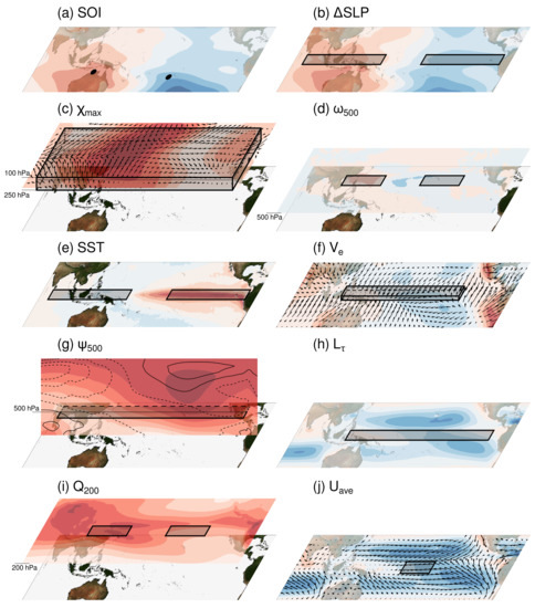
Figure 1.
Illustration of definitions of PWC indices. Plotted fields show average El niño state for each particular index and are meant to be just for illustrative purposes. Red shadings correspond to positive values and blue to negative. Black boxes represent areas for averaging and/or integration ( and ). For further explanation of definitions, see Section 2.1. (a) Anomalies in mean sea level pressure (contours every 0.25 hPa). Black points represent locations of Tahiti and Darwin. (b) Anomalies in mean sea level pressure (contours every 0.2 hPa). (c) Field of maximal deviation (in absolute value) of velocity potential from its zonal mean at 150 hPa (contours every ) and vectors of corresponding divergent wind. Black box represents the area inside which the maximal deviation of velocity potential is taken at every time step in order to compute the index. (d) Anomalies of at 500 hPa (contours every 0.015 Pa/s). (e) SST anomalies (contours every 0.2 K). (f) Vectors of effective wind for water vapor transport and magnitude of its zonal component (contours every 0.4 m/s). (g) Mass stream function from total wind (contours every ) and zonal wind (line contours every 4 m/s, negative values dashed), from 1000 to 100 hPa. (h) Zonal wind stress (contours every 0.025 N/m). (i) Specific humidity at 200 hPa (contours every 0.01 g/kg). (j) vectors of average surface wind and zonal wind speed (contours every 2 m/s).
2.1. Definitions of Indices
The following indices of Pacific Walker circulation are compared:
- 1.
- Point-based Southern oscillation index (SOI) from Troup [43]. The index is defined as the anomaly in the mean sea-level pressure difference between the Tahiti and Darwin stations (Figure 1a). The data are standardized for each month of the year using 1950–2021 as a base period. The closest model gridpoints are used for evaluation when computing the SOI from the reanalysis data (see Supplementary Information Figure S1 for justification).
- 2.
- Area-averaged Southern oscillation index ΔSLP from Vecchi et al. [31]. This index is defined as the difference between anomalies in mean sea-level pressure over the eastern and western equatorial Pacific (Figure 1b). The anomalies are calculated by averaging over two boxes, both extending from 5° S to 5° N in the meridional directions, and in the zonal direction from 80° E to 160° E (western Pacific box) and from 80° W to 160° W (eastern Pacific box). This index has widely been used due to the availability of long-term historical data on sea-level pressure.
- 3.
- Velocity potential index from Tanaka et al. [44]. The index is computed for 2D circulation at a single vertical level (typically pressure p level) by solving the Poisson equation:The index was originally defined by Tanaka et al. [44] as the yearly average of the maximum deviation of velocity potential from its zonal mean over the equatorial Pacific at 200 hPa level, between 25° S and 25° N, and 80° E and 80° W (named χ200). Here, the yearly averaging was applied as a 12-month running mean. As the maximum divergent outflow from a convective area over the Maritime continent is higher up in the troposphere (see Figure 2) and varies year-to-year, we constructed a data-adaptive index χmax that takes the maximal deviation of velocity potential from its zonal mean over the equatorial Pacific inside the box between 25° S and 25° N, and 80° E and 80° W, and 250 and 100 hPa at each time step as shown in Figure 1c. The justification of the index revision is described in Section 3.
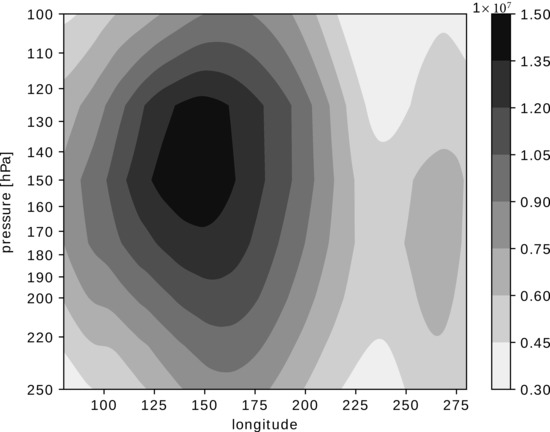 Figure 2. Maximal absolute value of (in s) between 25 S and 25 N, in the upper troposphere over equatorial Pacific, averaged over 1951–2020.
 - 4.
- Vertical velocity index from Wang [45] (named ω500). The index is calculated as the difference in average vertical pressure velocity anomalies between the eastern and western equatorial Pacific at 500 hPa (Figure 1d). The eastern Pacific is defined as an area between 120° W and 160° W, and from 5° S to 5° N. The western Pacific is defined between 120° E and 160° E, and from 5° S to 5° N.
- 5.
- The sea-surface temperature (SST) index is defined as the east-west difference in the SST, the same way as the ΔSLP index, but for the SST data (Figure 1e). The east-west SST gradient in the equatorial Pacific is strongly coupled to PWC through the Bjerknes feedback, and thus the SST data are often used as a proxy for the PWC strength [19,35,38,46].
- 6.
- Effective wind for the water vapor transport index following Sohn and Park [12]. The boundary layer easterlies in the lower return branch of the Walker circulation transport the water vapor from the eastern to the western Pacific to provide additional fuel for condensation heating, which maintains the Walker circulation. An increase or decrease in water vapor flux normalized by the total amount of vapor in the atmospheric column is regarded as the strengthening or weakening of circulation, respectively. The effective wind is defined aswhere PW(i) is precipitable water in a layer between the i-th and i + 1-th vertical levels, TPW is the total precipitable water in a column, and VD(i) is divergent wind at the i-th vertical level. The summation goes from the ground level upwards, in our case from 1000 hPa to 850 hPa (Figure 1f).Precipitable water is calculated aswhere is the water density, g is the gravity acceleration, is specific humidity, and and are boundaries of specific layer (). Total precipitable water is calculated in the same way, but the integration is done from (surface pressure) to the top of the atmosphere (). As we are interested in Walker circulation, we only used the zonal component of the divergent wind () and defined the index as an average value of effective zonal wind for water vapor transport in the tropical Pacific region from 120° E to 120° W, and from 5° S to 5° N, as demonstrated in Figure 1f.
- 7.
- Stream function index, based on the mass stream function:where a is the radius of the Earth, g is the gravity acceleration, and u is the zonal wind component averaged between 5° S and 5° N. We define the index (named ) as the maximal stream function at 500 hPa between 90° E and 80° W (Figure 1g). Originally, this index was defined using the zonal component of divergent wind [21,47,48]. In order to be able to align the index with other indices (which also include signals from other circulations), we opted for the zonal component of the total wind instead of its divergent part (their difference is shown in Figure 3).
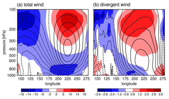 Figure 3. Vertical cross-section of the zonal wind (colors, in m/s) and the mass stream function (contours), averaged over the period 1950–2021 and over an area from 5 S to 5 N; (a) for total wind (contours every 2 × 10 kg/s) and (b) for divergent wind (contours every 0.4 × 10 kg/s).
 - 8.
- Zonally integrated (across the Pacific basin) wind stress following Clarke and Lebedev [49]. The index is defined aswhere is meridionally averaged zonal wind stress. Zonal integration is performed between 124° E and 90° W (Figure 1h). In the meridional direction, we chose to average between 5° S and 5° N to be consistent with other indices. Following Clarke and Lebedev [49], we computed wind stress aswhere is the air density (with a constant value of 1.2 kg/m as in Clarke and Lebedev [49]), is the drag coefficient (1.5 × 10), and is the horizontal surface wind vector at 10 m elevation ().
- 9.
- Upper-tropospheric specific humidity (denoted ). The deep convection in the ascending branch of the PWC transports the water vapor into the upper troposphere. Therefore, a change in the upper-tropospheric humidity may indicate a change in the circulation strength [13]. To eliminate the increase in specific humidity (a general increase in humidity due to global atmospheric warming), we formulated the index as the difference in upper tropospheric humidity at the top of the ascending and descending branches of Walker circulation. The Q200 PWC index is then defined as the difference in average specific humidity between two boxes over the eastern and western Pacific at 200 hPa (Figure 1i). We used the same horizontal boxes for specific humidity as those used for ω500.
- 10.
- Average surface zonal winds over the central equatorial Pacific (denoted Uave), after Chung et al. [23]. The index is applied by averaging 10 m wind over an area from 6° S to 6° N and from 180° to 150° W (Figure 1j).
2.2. Comparison of Distinct PWC Indices
The ten PWC indices can be grouped into two categories: (a) the direct circulation indices (χmax, ψ500, Lτ, Uave, Ve and ω500) that directly measure the velocity of the flow or associated flow function in any of the PWC branches, and (b) the indirect indices of the PWC magnitude derived from the atmospheric mass field or the lower boundary (Q200, SOI, ΔSLP and SST). The Q200 index measures PWC strength through the convective humidity-influx in the upper troposphere, whereas the SST index measures the PWC strength through coupled ocean–atmosphere interactions.
All indices described here are influenced also by other parts of the tropical general circulation, i.e., by the Hadley and Monsoon circulations [50,51,52]; however, the partitioning of dynamic field between different parts of the global circulation, e.g., [53,54,55], is beyond the scope of this study. The anthropogenic warming of the atmosphere and ocean, and increasing tropospheric water vapor directly affect the thermodynamic indices of PWC. For example, the increasing amount of water vapor in the tropical atmosphere increases the horizontal water vapor transport [30] and results in upper-tropospheric moistening [56], despite the reduced convective mass flux in the ascent regions [30,57].
The indices of PWC, described in the previous section, cannot be directly compared, as most of them attain physical units (ΔSOI, χ, ω500, SST, Ve, ψ, Lτ, Q200, Uave), whereas SOI is dimensionless by definition, and they can also span over different orders of magnitude. To make the indices comparable, we normalize them as in Equation (7):
where is the normalized index at time t, is the index value at time t, is the mean value of the index within the analyzed time frame and is the standard deviation of the index within the analyzed time frame.
The indices require different amounts of data for their evaluation. SOI is calculated from pressure measured at two particular locations and can thus be affected by the local microclimate, especially when computed directly from the station measurements. On the contrary, the indices from area-averaged data (SLP, , SST, , , , ) should better represent the changes of large-scale circulation. Some of the indices require onlyly one basic variable and are easily calculated (e.g., SOI, SLP, SST, , ), while others require derived products (e.g., , , , ) and/or more complex calculation (e.g., , ). It is, therefore, logical that, historically, the choice of the PWC index was influenced by the availability of data and computational resources.
2.3. Data
A dataset based on fully coupled atmosphere–ocean modeling, that is verified with observations, is required to intercompare a range of PWC indices. The latest ERA5 reanalysis, covering the period 1950–2021 [42,58,59], fulfills this requirement. The indices are derived from the pressure vertical velocity , the zonal and meridional winds and specific humidity, all provided on a regular latitude-longitude grid with 1 horizontal resolution and 27 vertical pressure levels from 100 to 1000 hPa. Sea surface temperature (SST) data and the mean-sea-level pressure (MSLP) data are used at the same horizontal grid [60,61]. Monthly means are computed from either daily 00 UTC data for horizontal winds or daily means for other variables. The mixed use of 00 UTC and daily mean data is justified by comparison of both datasets for the index at 500 hPa; however, the choice of 00 UTC or daily mean data has a negligible impact on the indices (see Figure S2).
We consider ERA5 to be sufficient for the analysis for several reasons. Simmons [62] showed that ERA5 verifies well with upper-tropospheric wind measurements in the tropics, with mean departure between observations and background or first-guess in data assimilation (i.e., short-range forecasts) for upper-tropospheric zonal winds being less than 1 m/s from the late 1990s onward. In addition, the supplemental material includes our verification of PWC indices based on surface winds in ERA5 and the independent wave- and anemometer-based sea surface wind product WASWind, [63] showing their close correspondence (Figure S3). The ERA5-derived SST indices also agree well with indices derived from HadISST data ([37]; see Figure S4 for comparison). The same applies to the SOI index based on ERA5 data, which has been verified against the index derived from raw station data. Similarly, the SLP index computed from ERA5 data accurately verifies against the index derived from HadSLP2 data [64] (for verification of both indices against observational datasets, see Figure S1).
In this study, the raw indices are computed for the 1950–2021 period. However, applying the 12-month running mean to the raw index values, as was done for the index, shortens its time series for six months at each end of the time frame. Therefore, we performed the comparison of indices for the 1951–2020 period.
The data analysis was performed using the following set of statistical tools. The spectral analysis was conducted on normalized monthly mean data using discrete Fourier transform. The spectral transform coefficients were then used to compute the power spectral density of time series of indices.
The correlation analysis was carried out by computing the Pearson correlation coefficient, which measures how the time series of two PWC indices (linearly) co-vary over time. We computed the Pearson correlation coefficients for time series of annual-mean index values. The null hypothesis of no correlation () was tested at the 0.05 significance level. The correlation analysis was performed using the pearsonr method from scipy.stats library [65]. Lead–lag relationships between the indices’ time series were not explored, as the indices are expected to reflect the realization of the same process.
The linear trends of PWC indices were computed as linear regression on time series of normalized annual-mean indices, using the linregress method from scipy.stats library [65]. Their statistical significance was tested with the modified, trend free, pre-whitening Mann–Kendall test from the Pymannkendall package [66,67].
3. Results
In this section, we present an analysis of the temporal evolution of the ten indices, including two revised indices. We also calculate the correlation coefficients between various indices. This is followed by an evaluation of trends and sensitivity analysis of the trends based on the period used for computation.
3.1. Time-Series of PWC Indices and Their Correlations
The time series of the normalized annual-mean PWC indices shown in Figure 4a demonstrate relatively good agreement in the evolution and relative strength of PWC during most of the period since 1950. Most of the indices spot strong El Niños in, for example, 1972, 1982/83, 1987, 1992, 1997/98, and 2015. The two indices that deviate most from the others are the stream function index based on the divergent zonal wind at 500 hPa and velocity potential at 200 hPa. Their poor agreement with other indices motivated their reformulation as described in the previous section and discussed further below.
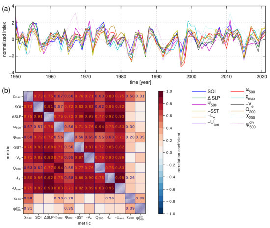
Figure 4.
(a) Time series of annual-mean PWC strength in ERA5 reanalysis between 1950 and 2021 for different PWC indices described in Section 2.1 as shown in the legend. (b) Correlations between annual means of different PWC indices. Statistically significant (at 95 % confidence level) correlation coefficients are written in the respective fields. The SST, , and indices are multiplied by (−1) for easier comparison with other indices. The and are shown dashed in (a), as they are replaced by better-defined equivalent indices and not used in the continuation.
For a more detailed view on the agreement of indices during El Niño/La Niña periods, monthly data should be examined (Figure 5). Generally, there is no clear link between the spread of indices and El Niño/La Niña periods, except for the three strongest El Niños in 1982/83, 1997/98 and 2015, when the spread clearly increased. The spread is also persistently higher in the 1950–1960 period, likely due to insufficient data coverage and the associated uncertainty in the ERA5 dataset prior to 1960.
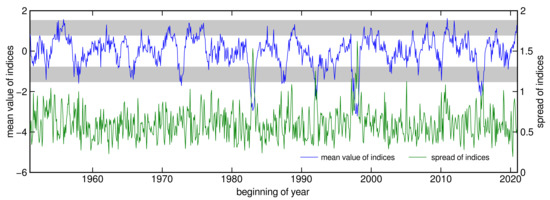
Figure 5.
Mean of normalized indices (without and ) and their spread. Both on monthly data. Area between one and two standard deviations from zero mean value is shaded gray.
By comparing the index values during El Niños and their mean climatological values (Figure S9), we find that some indices are more susceptible to interannual ENSO variability than others: during the strongest El Niños, , , and the SOI index show relatively smaller deviations from their respective mean index values than other indices. On the other hand, the Q, and indices show larger deviations from their respective mean.
Spectral analysis of monthly data (Figure 6) confirms that most of the indices have a strong signal in a 3.5-year period and 5-year period, representing the ENSO variability. Note that the SST index peaks at both periods among all PWC indices. Another smoothed spectral peak is observed at periods between 10 and 15 years in the SST and indices, which could be associated with the internal Pacific climate variability [68,69], whereas the sharp spectral peak at a 11-year period in other PWC indices may be associated with the 11-year solar cycle. However, different studies on the possible connection between Walker circulation and solar activity gave mixed conclusions [70,71,72,73]. To conclude, the large deviations of index values associated with the strong El Niños require caution when performing trend analysis. Whenever estimating long-term trends or inspecting the time series for multidecadal variability, one needs to (a) filter the ENSO variability from time series of indices as in, for example, [20], or (b) choose such a time interval that the strong El Niños do not occur at the beginning or the end of PWC time series, or (c) inspect the PWC strength over multiple time intervals in order not to skew the analysis (see also Section 3.3).
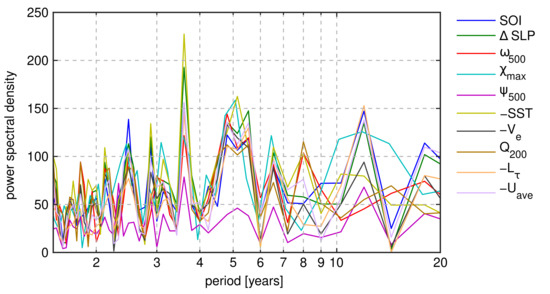
Figure 6.
Spectral analysis of time series of normalized indices, on monthly data.
The different indices that describe various aspects of PWC have varying correlations (Figure 4b). Correlations between indices derived from physically linked processes are generally high. For example, the pair of indices with the highest correlation coefficient () is and , which both describe surface easterlies. The index has a very high correlation () with the Q-index, as the amount of upper tropospheric humidity is directly related to the magnitude of vertical water vapor transport through convective mass flux. Similarly, the SLP index has a very high correlation ( to ) with the zonal surface wind index , the surface wind stress index , and the zonal boundary-layer moisture transport (represented by the effective wind ). This is expected, as the pressure difference (expressed by SOI, SLP) over the Pacific drives the near-surface equatorial easterlies. The more significant the pressure difference, the stronger the easterlies (), the wind stress (), and the water vapor transport (). The result confirms that the normalization in the index definition by the total water vapor successfully eliminates the global warming signal, which increases the global lower tropospheric moisture content through Clausius–Clapeyron scaling [30].
The correlations are somewhat lower between indices derived from distinct processes, for example, surface wind and upper-tropospheric humidity (). Moderate correlations are observed between , and SST and SLP indices with and , respectively. This suggests that the convective mass flux over the Maritime continent is controlled not only by the zonal SST gradient or associated SLP gradient, but also by the local meridional gradients in the western Pacific [50], as well as static stability and radiative cooling [30,57]. This is further supported by a rather moderate correlation () between the SST and indices.
The original index [44] and stream-function index [21,47] (both indicated with dashed line in Figure 4a) stand out from the rest and do not capture the strongest El Niños. After the year 2000, the -index also significantly exceeds the values of other indices. The velocity potential index is highly susceptible to the choice of upper-tropospheric pressure level (Figure 7), which is related to the strong vertical profile of the divergent outflow (Figure 2). The peak divergent outflow also occurs at different pressure levels year to year. Therefore, an index defined at some predetermined pressure level can miss the peak velocity potential in certain years. To alleviate it, we constructed a data-adaptive index, which takes the maximum of monthly mean at any level within the box area (defined in Section 2.1). This index correlates almost perfectly with the index (), meaning that the original velocity potential index () was applied too low in the troposphere. Our reformulated index verifies much better with other PWC indices (Figure 4b), and thus we suggest the reader to use the latter.
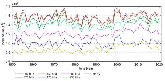
Figure 7.
Time series of annual-mean values of index at different vertical levels.
The stream-function index that is computed from the total zonal wind instead of the zonal divergent wind (as the original index is computed) also verifies better with the other PWC indices. The original index deviates from other PWC indices, particularly in the pre-satellite era in the 1960s and 1970s (see Figure 4a and Figure 8). Its correlations with other indices are small, and the only statistically significant correlations for annual means are with , and indices (r between 0.3 and 0.4), as shown in Figure 4b. For this reason and the reasons discussed in Section 2.1, we recommend the reader to use the revised stream-function index that is derived from the total zonal wind.
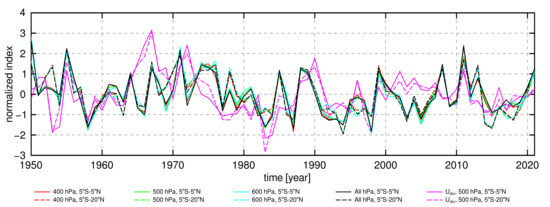
Figure 8.
Time series of different variations of normalized index from total zonal wind (annual means), at different vertical levels and for different meridional extent of areas over which wind was averaged. Vertical pressure level stands for indices computed as maximal mass stream function at a particular level, “All hPa” denotes index, computed as maximal stream function in the zonal-vertical cross-section, and “” denotes index, computed from the divergent component of zonal wind.
3.2. Sensitivity Analysis of PWC Indices
The PWC indices are typically defined at fixed vertical levels, where the underlying physical processes are the strongest on average. For example, the divergent outflow is strongest in the upper troposphere at around 150 hPa level (Figure 2), and the stream function has the largest amplitude at about the 500 hPa level. However, as the PWC strength and position oscillate on a year-to-year basis, the intercomparison of PWC indices may be skewed due to the displacement of maxima from the vertical levels on which indices are computed, as discussed in the previous subsection using the example of the index. To ensure that our results are not significantly affected by such displacements, we tested the sensitivity of the indices to meaningful changes in the vertical level. We examined this sensitivity for , , , and Q indices (see Figure 7, Figure 8, Figures S2 and S5). As tropical processes are mainly centered at the Inter-Tropical Convergence Zone (ITCZ), we also examined how the indices, originally defined in a narrow equatorial belt (5 S and 5 N) change when meridional borders of the areas considered are modified (e.g., 5 N and 20 N) to better align with the average position of the ITCZ. This was applied to , , , and Q indices (see Figures S6, Figure 8, Figures S7 and S5, respectively). In general, the indices are not very sensitive to the vertical level or horizontal area used for calculation, as long as the chosen level/area is similar to the level/area used in the original definition. This is supported by high-correlation coefficients between different variations of each index (not shown). The only exception is the index, which varies significantly with the vertical level used for computation, as already mentioned. Our sensitivity analysis confirms that the results on the PWC changes presented in this paper are not meaningfully impacted by mild shifts of vertical levels or meridional averaging.
3.3. Trends in PWC and Their Sensitivity to the WC
The PWC trends are analyzed using linear regression on time series of standardized annual-mean PWC indices. Figure 9 shows trends that start from various years from 1951 to 2000, with the end year of the time period fixed to 2020. The majority of the indices show neutral-to-negative trends for the starting years between 1951 and 1970, indicating that PWC has remained steady or has slightly been weakening over the past 70 to 50 years, in line with the conclusions of Kociuba and Power [14] based on the SLP index. Exceptions to this rule include the velocity-potential index and the SST index, which show the strengthening of PWC until the late 20th century. From 1980 to 2020, most indices suggest PWC strengthening. However, only the , and indices show statistically significant strengthening at the 95% confidence level (see Table 1). Similar conclusions apply also to the period between 1990 and 2020, where only five of the analyzed indices show statistically significant trends. In the most recent two decades (2000–2020 period), the majority of the indices suggest PWC weakening, although the uncertainty is relatively large.
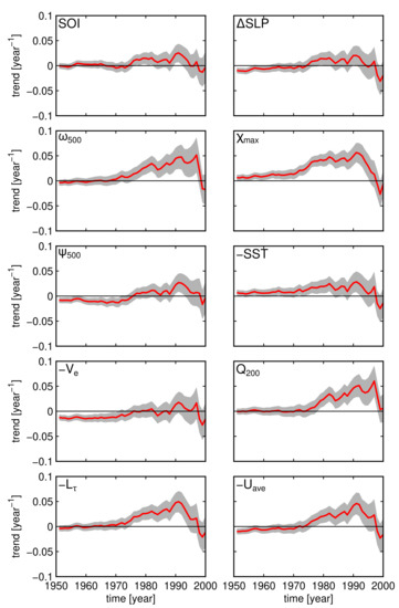
Figure 9.
Trends of Pacific Walker circulation (PWC) strength as a function of the starting year of the trend for different PWC indices. The end year of all linear trends is fixed to 2020. For example, the year 1970 on the x-axis represents the PWC trend calculated for 1970–2020. PWC trends for periods shorter than 20 years are not shown. Thick red lines represent the trend value, and the gray areas represent the uncertainty (i.e., plus or minus one standard deviation) of the estimated trend. SST, , and indices are multiplied by (−1) for easier comparison with other indices.

Table 1.
Trends of normalized indices of annual-mean Pacific Walker circulation strength for different periods shown in Figure 9 and Figure 10. The values in parentheses denote the standard error of the trend estimates. Stars denote a statistically significant trend at 95% confidence using the Mann–Kendall test. SST, , and indices are multiplied by (−1) for easier comparison with other indices. Units in columns denote linear trend (± 1 ) in units yr.
The question that arises next is how the trends change when we vary both the start year and the end year for the trend computation. This is illustrated in Figure 10. Three distinct areas can be identified in the figure, although they are not equally clear for all ten indices: (1) trends that start in the 1950s and end in the 1970s are mostly positive, indicating an increase in PWC strength; (2) trends that start approximately between 1960 and 1980, and end around 2010, are mostly negative and often statistically significant, suggesting a weakening of PWC; (3) trends that start between around 1980 and mid-to-late 1990s are again mostly positive, regardless of the end year. On the other hand, long-term trends that start before the mid-1970s and end after 2010 are insignificant and have even different signs. One can also notice semi-periodic white stripes, which are associated with the dominant ENSO variability and can skew our analysis of the long-term trends if the time frame for the trend evaluation is chosen arbitrarily.
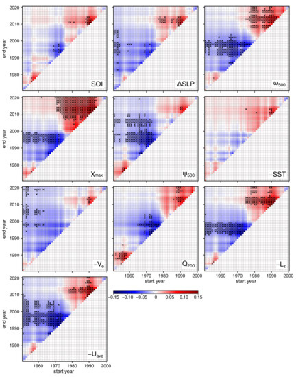
Figure 10.
Trends of Pacific Walker circulation (PWC) strength as a function of the starting year (x-axis) and end year (y-axis) of the trend for different PWC indices, similar as in [23]. PWC trends for periods shorter than 20 years are not shown. Crosses represent statistically significant trends at the 95% confidence level. SST, and indices are multiplied by (−1) for easier comparison with other indices. The checkered pattern is a result of ENSO variability. The first row in the matrix is a realization of Figure 9. The bottom-left top-right diagonal (0-diagonal) effectively represents a 20-year running trend, as in e.g., [20], whereas the k-diagonal represents a -year running trend.
The right diagonal line in any plot in Figure 10 shows 20-year running trends with start years from 1951 to 2000 (additionally plotted in Figure 11b). The variability of trends along this diagonal for most indices (except for point-based SOI) hints at possible 35-year multidecadal variability of the PWC: the early uptrend (red colours) is followed by approximately 16–20 years of downtrend (blue colors, start years 1963 to 1980), followed again by 16–20 years of uptrend (start years 1980 to 1996) and turning into a downtrend again (start year 1996). This hints at a multidecadal variability of the PWC with an approximately 35-year period which can also be seen in the 20-year running mean (Figure 11a). If so, blue patches in the upper-right corners of Figure 10 that indicate a PWC weakening, together with recent trends in Figure 9, suggest that a multidecadal trend reversal might be taking place. Although further analysis with a longer dataset is needed to confirm that the trends are associated with a multidecadal oscillation in PWC, our expectation of a weakened PWC in the coming years agrees with Wu et al. [33], who reached their conclusion by coupling the PWC with the interdecadal Pacific oscillation.
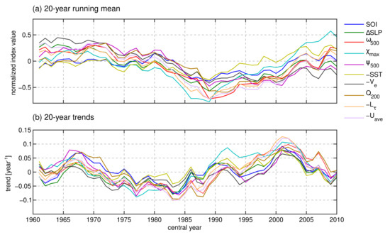
Figure 11.
(a) The 20-year running mean of normalized annual-mean index values and (b) 20-year running trends of normalized annual-mean index values. The x-axis defines the central year of running mean and trends.
4. Discussion and Conclusions
The study reviewed and compared ten different indices of the Pacific Walker circulation (PWC) strength over the 1951–2020 period using the ECMWF ERA5 reanalyses. We demonstrated that the indices derived from ERA5 are equivalent to indices deduced from the raw observation data. It was already shown before that ERA5 accurately verifies the observations of upper-tropospheric zonal winds, zonal surface winds, sea-level pressure, and sea-surface temperature (see Supplementary Information and [42,62]), which makes it compelling to use in the studies of climate change and climate dynamics.
We showed that the sensitivity of indices to reasonable changes in the choice of vertical level or horizontal averaging area is negligible. One exception is the velocity potential index, which displays strong sensitivity to the choice of the vertical level at which the index is computed. The index was originally defined at 200 hPa [44], but the newest state-of-the-art datasets suggest that the maximum divergent outflow associated with convection over the western Pacific is higher in the troposphere, at around 150 hPa. Similarly, the original definition of the stream function index is based on divergent wind [21,47] and, in comparison to other common PWC indices, misses an important part of the zonal tropical circulation associated with the PWC. Therefore, in this study, we argued to replace and indices with a data-adaptive index, and a stream-function index derived from the total zonal wind, respectively.
We showed that the normalized PWC indices agree regarding the variation of annual-mean PWC strength (see Figure 4a). The correlations are highest ( or more) between the indices that describe closely linked processes, as could be expected. The discrepancies among indices, i.e., their spread, are the largest during the strong El Niño events. The ENSO variability dominates the PWC variability; therefore, we argue that the estimation of PWC trends and long-term variability should ideally be based on ENSO-filtered time series. Alternatively, indices that display lower sensitivity to ENSO could be used, such as , , and SOI, or, a range of possible time periods should be considered to establish firm conclusions on trends, as shown in Figure 9 and Figure 10.
The sensitivity of trends to the applied time periods is often poorly explored in the literature. Our study shows that different indices, different lengths of the applied interval, and their start and end years, can greatly affect the trends and their significance. In the common climatological reference period 1981–2010, the majority of indices showed PWC strengthening. On a longer time scale, i.e., 1951–2020, the trend is mostly neutral and insignificant. Furthermore, the majority of indices suggest that the PWC might have been weakening during the last two decades (2000–2020). A continuation of this trend implies a reversal of the PWC into an El Niño-type state with decreased ocean heat uptake and more rapid global warming. We suggest that the observed variability in the trends of the PWC indices might be associated with the multidecadal variability of the PWC with a period of about 35 years. Longer data series are needed to confirm this result.
The recent (1981–2010) PWC strengthening is unequivocally opposed to climate model projections [74]. Whether the source of the discrepancy is multidecadal variability as seen in Figure 10 [19,23,33], forced response [75,76] or biases in the coupled ocean–atmosphere climate models [2,9,77,78,79], caution should be exercised for the detection and comparison of PWC trends in the models and reanalyses. We speculate a shift toward the weakening of the PWC. If realized, it will crucially impact the global distribution of precipitation in the tropics and extratropics, the ocean heat uptake, e.g., [7], the sea-level rise and the rate of global warming.
Supplementary Materials
The supporting information can be downloaded at: https://www.mdpi.com/article/10.3390/atmos14020397/s1. The supplementary information includes: comparison of Troup SOI computed from station data and derived from ERA5 data (Figure S1); comparison of SLP indices from HadSLP2 data and derived from ERA5 (Figure S1); comparison of indices computed at different vertical levels (Figure S2); comparison of indices computed from daily-mean ERA5 data and 00 UTC data (Figure S2); comparison of Uave index from ERA5 and WASWind data (Figure S3); comparison of SST index from ERA5 and HadISST data (Figure S4); comparison of Q index, computed at different vertical levels and for various horizontal areas (Figure S5); comparison of V index, computed on different horizontal areas (Figure S6); comparison of different variations of L index (Figures S7 and S8, which include references to [49,80]); comparison of monthly time series of normalized indices and their multi-index mean (Figure S9).
Author Contributions
Both authors (K.K. and Ž.Z.) contributed equally in activities leading to the production of this article. Conceptualization, Ž.Z.; methodology, K.K., Ž.Z.; software, K.K.; formal analysis, K.K., Ž.Z.; investigation, K.K, Ž.Z.; data curation, K.K., Ž.Z.; verification, K.K., Ž.Z.; writing—original draft preparation, K.K., Ž.Z.; writing—review and editing, K.K., Ž.Z.; visualization, K.K.; supervision, Ž.Z.; project administration, K.K., Ž.Z.; funding acquisition, K.K., Ž.Z. All authors have read and agreed to the published version of the manuscript.
Funding
This research has been supported by the Javna Agencija za Raziskovalno Dejavnost RS (Slovenian Research Agency: grant no. J1-9431 and Program P1-0188).
Institutional Review Board Statement
Not applicable.
Informed Consent Statement
Not applicable.
Data Availability Statement
ERA5 data (https://doi.org/10.24381/cds.bd0915c6 accessed on 17 January 2023, [58,59,60,61]) was downloaded from the Copernicus Climate Change Service (C3S) Climate Data Store (last access 27 June 2022). The results contain modified Copernicus Climate Change Service information 2022. Neither the European Commission nor ECMWF is responsible for any use that may be made of the Copernicus information or data it contains. Scripts for calculation of indices and data used to generate Figure 1, Figure 2, Figure 3, Figure 4, Figure 5, Figure 6, Figure 7, Figure 8, Figure 9, Figure 10 and Figure 11 and S1–S9 are published in Zenodo data repository: https://doi.org/10.5281/zenodo.7359879 accessed on 17 January 2023.
Acknowledgments
The authors thank Nedjeljka Žagar (Meteorological Institute, Center for Earth System Research and Sustainability, Universität Hamburg) for carefully reading the manuscript and suggesting additional analysis, and Matic Pikovnik (Slovenian Environment Agency, ARSO, and University of Ljubljana, Faculty of Mathematics and Physics) for sharing parts of the code that contributed to this research.
Conflicts of Interest
The authors declare no conflict of interest. The funders had no role in the design of the study; in the collection, analyses, or interpretation of data; in the writing of the manuscript; or in the decision to publish the results.
References
- Peixoto, J.P.; Oort, A.H. Physics of Climate; American Institute of Physics: College Park, MD, USA, 1992; p. 520. [Google Scholar]
- Seager, R.; Cane, M.; Henderson, N.; Lee, D.E.; Abernathey, R.; Zhang, H. Strengthening tropical Pacific zonal sea surface temperature gradient consistent with rising greenhouse gases. Nat. Clim. cahnge 2019, 9, 517–522. [Google Scholar] [CrossRef]
- Bjerknes, J. Atmospheric Teleconnetions from the Equatorial Pacific. Mon. Weather Rev. 1969, 97, 163–172. [Google Scholar] [CrossRef]
- Barichivich, J.; Gloor, E.; Peylin, P.; Brienen, R.J.; Schöngart, J.; Espinoza, J.C.; Pattnayak, K.C. Recent intensification of Amazon flooding extremes driven by strengthened Walker circulation. Sci. Adv. 2018, 4, eaat8785. [Google Scholar] [CrossRef] [PubMed]
- Merrifield, M.A. A Shift in Western Tropical Pacific Sea Level Trends during the 1990s. J. Clim. 2011, 24, 4126–4138. [Google Scholar] [CrossRef]
- Muis, S.; Haigh, I.D.; Guimarães Nobre, G.; Aerts, J.C.; Ward, P.J. Influence of El Niño-Southern Oscillation on Global Coastal Flooding. Earth’s Future 2018, 6, 1311–1322. [Google Scholar] [CrossRef]
- Meehl, G.A.; Arblaster, J.M.; Fasullo, J.T.; Hu, A.; Trenberth, K.E. Model-based evidence of deep-ocean heat uptake during surface-temperature hiatus periods. Nat. Clim. cahnge 2011, 1, 360–364. [Google Scholar] [CrossRef]
- England, M.H.; Mcgregor, S.; Spence, P.; Meehl, G.A.; Timmermann, A.; Cai, W.; Gupta, A.S.; Mcphaden, M.J.; Purich, A.; Santoso, A. Recent intensification of wind-driven circulation in the Pacific and the ongoing warming hiatus. Nat. Clim. cahnge 2014, 4, 222–227. [Google Scholar] [CrossRef]
- McGregor, S.; Timmermann, A.; Stuecker, M.F.; England, M.H.; Merrifield, M.; Jin, F.F.; Chikamoto, Y. Recent walker circulation strengthening and pacific cooling amplified by atlantic warming. Nat. Clim. cahnge 2014, 4, 888–892. [Google Scholar] [CrossRef]
- Betts, R.A.; Burton, C.A.; Feely, R.A.; Collins, M.; Jones, C.D.; Wiltshire, A.J. ENSO and the Carbon Cycle. Geophys. Monogr. Ser. 2020, 253, 453–470. [Google Scholar] [CrossRef]
- Kosaka, Y.; Xie, S.P. Recent global-warming hiatus tied to equatorial Pacific surface cooling. Nature 2013, 501, 403–407. [Google Scholar] [CrossRef]
- Sohn, B.J.; Park, S.C. Strengthened tropical circulations in past three decades inferred from water vapor transport. J. Geophys. Res. 2010, 115, D15112. [Google Scholar] [CrossRef]
- Sohn, B.J.; Yeh, S.W.; Schmetz, J.; Song, H.J. Observational evidences of Walker circulation change over the last 30 years contrasting with GCM results. Clim. Dyn. 2013, 40, 1721–1732. [Google Scholar] [CrossRef]
- Kociuba, G.; Power, S.B. Inability of CMIP5 Models to Simulate Recent Strengthening of the Walker Circulation: Implications for Projections. J. Clim. 2015, 28, 20–35. [Google Scholar] [CrossRef]
- Zhou, Y.P.; Xu, K.M.; Sud, Y.C.; Betts, A.K. Recent trends of the tropical hydrological cycle inferred from Global Precipitation Climatology Project and International Satellite Cloud Climatology Project data. J. Geophys. Res. Atmos. 2011, 116, 9101. [Google Scholar] [CrossRef]
- Zahn, M.; Allan, R.P. Changes in water vapor transports of the ascending branch of the tropical circulation. J. Geophys. Res. Atmos. 2011, 116, 18111. [Google Scholar] [CrossRef]
- Chen, J.; Del Genio, A.D.; Carlson, B.E.; Bosilovich, M.G. The Spatiotemporal Structure of Twentieth-Century Climate Variations in Observations and Reanalyses. Part I: Long-Term Trend. J. Clim. 2008, 21, 2611–2633. [Google Scholar] [CrossRef]
- Luo, J.J.; Sasaki, W.; Masumoto, Y. Indian Ocean warming modulates Pacific climate change. Proc. Natl. Acad. Sci. USA 2012, 109, 18701–18706. [Google Scholar] [CrossRef]
- Meng, Q.; Latif, M.; Park, W.; Keenlyside, N.S.; Semenov, V.A.; Martin, T. Twentieth century Walker Circulation change: Data analysis and model experiments. Clim. Dyn. 2012, 38, 1757–1773. [Google Scholar] [CrossRef]
- L’Heureux, M.L.; Lee, S.; Lyon, B. Recent multidecadal strengthening of the Walker circulation across the tropical Pacific. Nat. Clim. cahnge 2013, 3, 571–576. [Google Scholar] [CrossRef]
- Bayr, T.; Dommenget, D.; Martin, T.; Power, S.B. The eastward shift of the Walker Circulation in response to global warming and its relationship to ENSO variability. Clim. Dyn. 2014, 43, 2747–2763. [Google Scholar] [CrossRef]
- Sandeep, S.; Stordal, F.; Sardeshmukh, P.D.; Compo, G.P. Pacific Walker Circulation variability in coupled and uncoupled climate models. Clim. Dyn. 2014, 43, 103–117. [Google Scholar] [CrossRef]
- Chung, E.S.; Timmermann, A.; Soden, B.J.; Ha, K.J.; Shi, L.; John, V.O. Reconciling opposing Walker circulation trends in observations and model projections. Nat. Clim. cahnge 2019, 9, 405–412. [Google Scholar] [CrossRef]
- Zhao, X.; Allen, R.J. Strengthening of the Walker Circulation in recent decades and the role of natural sea surface temperature variability. Environ. Res. Commun. 2019, 1, 021003. [Google Scholar] [CrossRef]
- Falster, G.; Konecky, B.; Madhavan, M.; Stevenson, S.; Coats, S. Imprint of the Pacific Walker Circulation in Global Precipitation δ18O. J. Clim. 2021, 34, 8579–8597. [Google Scholar] [CrossRef]
- Lee, S.; L’Heureux, M.; Wittenberg, A.T.; Seager, R.; O’Gorman, P.A.; Johnson, N.C. On the future zonal contrasts of equatorial Pacific climate: Perspectives from Observations, Simulations, and Theories. NPJ Clim. Atmos. Sci. 2022, 5, 82. [Google Scholar] [CrossRef]
- Watanabe, M.; Kamae, Y.; Yoshimori, M.; Oka, A.; Sato, M.; Ishii, M.; Mochizuki, T.; Kimoto, M. Strengthening of ocean heat uptake efficiency associated with the recent climate hiatus. Geophys. Res. Lett. 2013, 40, 3175–3179. [Google Scholar] [CrossRef]
- Bellomo, K.; Clement, A.C. Evidence for weakening of the Walker circulation from cloud observations. Geophys. Res. Lett. 2015, 42, 7758–7766. [Google Scholar] [CrossRef]
- Knutson, T.R.; Manabe, S. Time-mean response over the tropical Pacific to increased CO2 in a coupled ocean-atmosphere model. J. Clim. 1995, 8, 2181–2199. [Google Scholar] [CrossRef]
- Held, I.M.; Soden, B.J. Robust responses of the hydrological cycle to global warming. J. Clim. 2006, 19, 5686–5699. [Google Scholar] [CrossRef]
- Vecchi, G.A.; Soden, B.J.; Wittenberg, A.T.; Held, I.M.; Leetmaa, A.; Harrison, M.J. Weakening of tropical Pacific atmospheric circulation due to anthropogenic forcing. Nature 2006, 441, 73–76. [Google Scholar] [CrossRef]
- Vecchi, G.A.; Soden, B.J. Global Warming and the Weakening of the Tropical Circulation. J. Clim. 2007, 20, 4316–4340. [Google Scholar] [CrossRef]
- Wu, M.; Zhou, T.; Li, C.; Li, H.; Chen, X.; Wu, B.; Zhang, W.; Zhang, L. A very likely weakening of Pacific Walker Circulation in constrained near-future projections. Nat. Commun. 2021, 12, 1–8. [Google Scholar] [CrossRef] [PubMed]
- Masson-Delmotte, V.; Zhai, P.; Pirani, A.; Connors, S.; Péan, C.; Berger, S.; Caud, N.; Chen, Y.; Goldfarb, L.; Gomis, M.; et al. IPCC, 2021: Climate Change 2021: The Physical Science Basis. Contribution of Working Group I to the Sixth Assessment Report of the Intergovernmental Panel on Climate Change; Cambridge University Press: Cambridge, UK, 2021. [Google Scholar]
- Tokinaga, H.; Xie, S.P.; Deser, C.; Kosaka, Y.; Okumura, Y.M. Slowdown of the Walker circulation driven by tropical Indo-Pacific warming. Nature 2012, 491, 439–443. [Google Scholar] [CrossRef]
- Woodruff, S.D.; Worley, S.J.; Lubker, S.J.; Ji, Z.; Eric Freeman, J.; Berry, D.I.; Brohan, P.; Kent, E.C.; Reynolds, R.W.; Smith, S.R.; et al. ICOADS Release 2.5: Extensions and enhancements to the surface marine meteorological archive. Int. J. Climatol. 2011, 31, 951–967. [Google Scholar] [CrossRef]
- Rayner, N.A.; Parker, D.E.; Horton, E.B.; Folland, C.K.; Alexander, L.V.; Rowell, D.P.; Kent, E.C.; Kaplan, A. Global analyses of sea surface temperature, sea ice, and night marine air temperature since the late nineteenth century. J. Geophys. Res. Atmos. 2003, 108, 4407. [Google Scholar] [CrossRef]
- Deser, C.; Phillips, A.S.; Alexander, M.A. Twentieth century tropical sea surface temperature trends revisited. Geophys. Res. Lett. 2010, 37, L10701. [Google Scholar] [CrossRef]
- Power, S.B.; Kociuba, G. What Caused the Observed Twentieth-Century Weakening of the Walker Circulation? J. Clim. 2011, 24, 6501–6514. [Google Scholar] [CrossRef]
- DiNezio, P.N.; Vecchi, G.A.; Clement, A.C. Detectability of Changes in the Walker Circulation in Response to Global Warming. J. Clim. 2013, 26, 4038–4048. [Google Scholar] [CrossRef]
- Liu, Z.; Jian, Z.; Poulsen, C.J.; Zhao, L. Isotopic evidence for twentieth-century weakening of the Pacific Walker circulation. Earth Planet. Sci. Lett. 2019, 507, 85–93. [Google Scholar] [CrossRef]
- Hersbach, H.; Bell, B.; Berrisford, P.; Hirahara, S.; Horányi, A.; Muñoz-Sabater, J.; Nicolas, J.; Peubey, C.; Radu, R.; Schepers, D.; et al. The ERA5 Global Reanalysis. Q. J. R. Meteorol. Soc. 2020, 146, 1999–2049. [Google Scholar] [CrossRef]
- Troup, A.J. The ‘southern oscillation’. Q. J. R. Meteorol. Soc. 1965, 91, 490–506. [Google Scholar] [CrossRef]
- Tanaka, H.L.; Ishizaki, N.; Kitoh, A. Trend and interannual variability of Walker, monsoon and Hadley circulations defined by velocity potential in the upper troposphere. Tellus A 2004, 56, 250–269. [Google Scholar] [CrossRef]
- Wang, C. Atmospheric circulation cells associated with the El Nino-Southern Oscillation. J. Clim. 2002, 15, 399–419. [Google Scholar] [CrossRef]
- Zhang, L.; Karnauskas, K.B. The Role of Tropical Interbasin SST Gradients in Forcing Walker Circulation Trends. J. Clim. 2017, 30, 499–508. [Google Scholar] [CrossRef]
- Yu, B.; Zwiers, F.W. Changes in equatorial atmospheric zonal circulations in recent decades. Geophys. Res. Lett. 2010, 37, 5701. [Google Scholar] [CrossRef]
- Eresanya, E.O.; Guan, Y. Structure of the Pacific Walker Circulation Depicted by the Reanalysis and CMIP6. Atmosphere 2021, 12, 1219. [Google Scholar] [CrossRef]
- Clarke, A.J.; Lebedev, A. Long-Term Changes in the Equatorial Pacific Trade Winds. J. Clim. 1996, 9, 1020–1029. [Google Scholar] [CrossRef]
- Sohn, B.J.; Yeh, S.W.; Lee, A.; Lau, W.K. Regulation of atmospheric circulation controlling the tropical Pacific precipitation change in response to CO2 increases. Nat. Commun. 2019, 10, 1108. [Google Scholar] [CrossRef]
- Pikovnik, M.; Zaplotnik, Z.; Boljka, L.; Žagar, N. Metrics of the Hadley circulation strength and associated circulation trends. Weather Clim. Dyn. 2022, 3, 625–644. [Google Scholar] [CrossRef]
- Zaplotnik, Z.; Pikovnik, M.; Boljka, L. Recent Hadley circulation strengthening: A trend or multidecadal variability? J. Clim. 2022, 35, 4157–4176. [Google Scholar] [CrossRef]
- Schwendike, J.; Govekar, P.; Reeder, M.J.; Wardle, R.; Berry, G.J.; Jakob, C. Local partitioning of the overturning circulation in the tropics and the connection to the Hadley and Walker circulations. J. Geophys. Res. Atmos. 2014, 119, 1322–1339. [Google Scholar] [CrossRef]
- Hu, S.; Cheng, J.; Chou, J. Novel three-pattern decomposition of global atmospheric circulation: Generalization of traditional two-dimensional decomposition. Clim. Dyn. 2017, 49, 3573–3586. [Google Scholar] [CrossRef]
- Hu, S.; Chou, J.; Cheng, J. Three-pattern decomposition of global atmospheric circulation: Part I—decomposition model and theorems. Clim. Dyn. 2018, 50, 2355–2368. [Google Scholar] [CrossRef]
- Chung, E.S.; Soden, B.; Sohn, B.J.; Shi, L. Upper-tropospheric moistening in response to anthropogenic warming. Proc. Natl. Acad. Sci. USA 2014, 111, 11636–11641. [Google Scholar] [CrossRef]
- Jenney, A.M.; Randall, D.A.; Branson, M.D. Understanding the Response of Tropical Ascent to Warming Using an Energy Balance Framework. J. Adv. Model. Earth Syst. 2020, 12, e2020MS002056. [Google Scholar] [CrossRef]
- Hersbach, H.; Bell, B.; Berrisford, P.; Biavati, G.; Horányi, A.; Muñoz Sabater, J.; Nicolas, J.; Peubey, C.; Radu, R.; Rozum, I.; et al. ERA5 Hourly Data on Pressure Levels from 1959 to Present. Available online: https://cds.climate.copernicus.eu/cdsapp#!/dataset/10.24381/cds.bd0915c6?tab=overview (accessed on 27 June 2022).
- Bell, B.; Hersbach, H.; Berrisford, P.; Dahlgren, P.; Horányi, A.; Muñoz Sabater, J.; Nicolas, J.; Radu, R.; Schepers, D.; Simmons, A.; et al. ERA5 Hourly Data on Pressure Levels from 1950 to 1978 (Preliminary Version). 2020. Available online: https://cds.climate.copernicus.eu/cdsapp#!/dataset/reanalysis-era5-pressure-levels-preliminary-back-extension?tab=overview (accessed on 27 June 2022).
- Hersbach, H.; Bell, B.; Berrisford, P.; Biavati, G.; Horányi, A.; Muñoz Sabater, J.; Nicolas, J.; Peubey, C.; Radu, R.; Rozum, I.; et al. ERA5 Hourly Data on Single Levels from 1959 to Present. Available online: https://cds.climate.copernicus.eu/cdsapp#!/dataset/reanalysis-era5-single-levels?tab=overview (accessed on 27 June 2022).
- Bell, B.; Hersbach, H.; Berrisford, P.; Dahlgren, P.; Horányi, A.; Muñoz Sabater, J.; Nicolas, J.; Radu, R.; Schepers, D.; Simmons, A.; et al. ERA5 Hourly Data on Single Levels from 1950 to 1978 (Preliminary Version). Available online: https://cds.climate.copernicus.eu/cdsapp#!/dataset/reanalysis-era5-single-levels-preliminary-back-extension?tab=overview (accessed on 27 June 2022).
- Simmons, A.J. Trends in the tropospheric general circulation from 1979 to 2022. Weather Clim. Dyn. 2022, 3, 777–809. [Google Scholar] [CrossRef]
- Tokinaga, H.; Xie, S.P. Wave- and Anemometer-Based Sea Surface Wind (WASWind) for Climate Change Analysis. J. Clim. 2011, 24, 267–285. [Google Scholar] [CrossRef]
- Allan, R.; Ansell, T. A New Globally Complete Monthly Historical Gridded Mean Sea Level Pressure Dataset (HadSLP2): 1850–2004. J. Clim. 2006, 19, 5816–5842. [Google Scholar] [CrossRef]
- Virtanen, P.; Gommers, R.; Oliphant, T.E.; Haberland, M.; Reddy, T.; Cournapeau, D.; Burovski, E.; Peterson, P.; Weckesser, W.; Bright, J.; et al. SciPy 1.0: Fundamental Algorithms for Scientific Computing in Python. Nat. Methods 2020, 17, 261–272. [Google Scholar] [CrossRef]
- Yue, S.; Wang, C. Applicability of Prewhitening to Eliminate the Influence of Serial Correlation on the Mann-Kendall Test. Water Resour. Res. 2002, 38, 4-1–4-7. [Google Scholar] [CrossRef]
- Hussain, M.M.; Mahmud, I. pyMannKendall: A python package for non parametric Mann Kendall family of trend tests. J. Open Source Softw. 2019, 4, 1556. [Google Scholar] [CrossRef]
- Zhang, Y.; Wallace, J.M.; Battisti, D.S. ENSO-like Interdecadal Variability: 1900–93. J. Clim. 1997, 10, 1004–1020. [Google Scholar] [CrossRef]
- Mantua, N.J.; Hare, S.R.; Zhang, Y.; Wallace, J.M.; Francis, R.C. A Pacific Interdecadal Climate Oscillation with Impacts on Salmon Production*. Bull. Am. Meteorol. Soc. 1997, 78, 1069–1080. [Google Scholar] [CrossRef]
- Van Loon, H.; Meehl, G.A.; Shea, D.J. Coupled air-sea response to solar forcing in the Pacific region during northern winter. J. Geophys. Res. Atmos. 2007, 112, D02108. [Google Scholar] [CrossRef]
- Roy, I.; Haigh, J.D. Solar Cycle Signals in the Pacific and the Issue of Timings. J. Atmos. Sci. 2012, 69, 1446–1451. [Google Scholar] [CrossRef]
- Misios, S.; Gray, L.J.; Knudsen, M.F.; Karoff, C.; Schmidt, H.; Haigh, J.D. Slowdown of the Walker circulation at solar cycle maximum. Proc. Natl. Acad. Sci. USA 2019, 116, 7186–7191. [Google Scholar] [CrossRef]
- Roy, I. Is it always slowdown of the Walker circulation at solar cycle maximum? Nat. Hazards 2021, 107, 2021–2026. [Google Scholar] [CrossRef]
- Gulev, S.K.; Thorne, P.W.; Ahn, J.; Dentener, F.J.; Domingues, C.M.; Gerland, S.; Gong, D.; Kaufman, D.S.; Nnamchi, H.C.; Quaas, J.; et al. Changing State of the Climate System. In Climate Change 2021: The Physical Science Basis. Contribution of Working Group I to the Sixth Assessment Report of the Intergovernmental Panel on Climate Change; Masson-Delmotte, V., Zhai, P., Pirani, A., Connors, S.L., Péan, C., Berger, S., Caud, N., Chen, Y., Goldfarb, L., Gomis, M.I., et al., Eds.; Cambridge University Press: Cambridge, UK; New York, NY, USA, 2021; Chapter 2. [Google Scholar]
- Mann, M.E.; Steinman, B.A.; Brouillette, D.J.; Miller, S.K. Multidecadal climate oscillations during the past millennium driven by volcanic forcing. Science 2021, 371, 1014–1019. [Google Scholar] [CrossRef]
- Orihuela-Pinto, B.; England, M.H.; Taschetto, A.S. Interbasin and interhemispheric impacts of a collapsed Atlantic Overturning Circulation. Nat. Clim. cahnge 2022, 12, 558–565. [Google Scholar] [CrossRef]
- Durack, P.J.; Wijffels, S.E.; Matear, R.J. Ocean salinities reveal strong global water cycle intensification during 1950 to 2000. Science 2012, 336, 455–458. [Google Scholar] [CrossRef]
- Watanabe, M.; Dufresne, J.L.; Kosaka, Y.; Mauritsen, T.; Tatebe, H. Enhanced warming constrained by past trends in equatorial Pacific sea surface temperature gradient. Nat. Clim. cahnge 2020, 11, 33–37. [Google Scholar] [CrossRef]
- Wills, R.C.J.; Dong, Y.; Proistosecu, C.; Armour, K.C.; Battisti, D.S. Systematic Climate Model Biases in the Large-Scale Patterns of Recent Sea-Surface Temperature and Sea-Level Pressure Change. Geophys. Res. Lett. 2022, 49, e2022GL100011. [Google Scholar] [CrossRef]
- Wright, D.G. and Thompson, K.R. Time-Averaged Forms of the Nonlinear Stress Law. J. Phys. Oceanogr. 1983, 13, 341–345. [Google Scholar] [CrossRef]


Disclaimer/Publisher’s Note: The statements, opinions and data contained in all publications are solely those of the individual author(s) and contributor(s) and not of MDPI and/or the editor(s). MDPI and/or the editor(s) disclaim responsibility for any injury to people or property resulting from any ideas, methods, instructions or products referred to in the content. |
© 2023 by the authors. Licensee MDPI, Basel, Switzerland. This article is an open access article distributed under the terms and conditions of the Creative Commons Attribution (CC BY) license (https://creativecommons.org/licenses/by/4.0/).