Mind the Large Gap: Novel Algorithm Using Seasonal Decomposition and Elastic Net Regression to Impute Large Intervals of Missing Data in Air Quality Data

Abstract

Air quality data sets are widely used in numerous analyses. Missing values are ubiquitous in air quality data sets as the data are collected through sensors. Recovery of missing data is a challenging task in the data preprocessing stage. This task becomes more challenging in time series data as time is an implicit variable that cannot be ignored. Even though existing methods to deal with missing data in time series perform well in situations where the percentage of missing values is relatively low and the gap size is small, their performances are reasonably lower when it comes to large gaps. This paper presents a novel algorithm based on seasonal decomposition and elastic net regression to impute large gaps of time series data when there exist correlated variables. This method outperforms several other existing univariate approaches namely Kalman smoothing on ARIMA models, Kalman smoothing on structural time series models, linear interpolation, and mean imputation in imputing large gaps. However, this is applicable only when there exists one or more correlated variables with the time series with large gaps.

1. Introduction

Air quality is one of the environmental determinants of population health. Exposure to poor air quality is associated with numerous adverse health effects. Studies have shown that exposure to particulate and gaseous pollutants may lead to increased risk of cardiovascular and respiratory morbidity and mortality [1,2,3,4]. Common air pollutants include carbon monoxide (CO), nitrogen oxide (NO), nitrogen dioxide (NO${}_2$), ozone (O${}_3$), sulfur dioxide (SO${}_2$), and particulate matter less than 2.5 $\mathsf{\mu }$m (PM${}_{2.5}$) and 10 $\mathsf{\mu }$m (PM${}_{10}$) in aerodynamic diameter. Analyses of these pollutants play an important role in managing and mitigating adverse health effects due to poor air quality.

Measurements of air quality variables (pollutants) are recorded using environmental sensors. Data collected through sensors often exhibit missing data due to failures of the devices. Most of the analysis techniques rely on complete data sets. For example, in time series, some of the methods for decomposing a time series would not work with missing data. Therefore, dealing with missing values plays an inevitable role in prepossessing air quality data sets. Unless carefully dealt with, missing values may introduce a substantial bias for the analysis. The most desired thing is to have a complete data set for the required analysis. However, in reality, this is often not the case.

There are three types of missing mechanisms namely Missing Completely at Random (MCAR), Missing at Random (MAR) and Missing Not at Random (MNAR) [5]. Let $Y={(y_1,\dots ,y_n)}^T$ denote a vector of complete data set with both observed ($Y_{obs}$) and the missing values ($Y_{mis}$) with probability density function $f_{\theta }$. The objective is to make inferences about the vector of the unknown parameter $\theta$. The missing indicator, $M={(M_1,\dots ,M_n)}^T$ defines a binary variable that denotes whether the value of a variable is observed or missing (i.e., $M_i=0$ if value $y_i$ is observed and $M_i=1$ if the value is missing). The conditional distribution of M given the complete data $Y,f(M/Y,\varphi )$ describes the missing data mechanism where $\varphi$, denotes the vector of unknown parameters that describe the probability of missing data [6].

MCAR:

$$P\left(M\right|Y_{obs},Y_{mis},\varphi )=P\left(M\right|\varphi )forallY,\varphi$$

(1)

MAR:

$$P\left(M\right|Y_{obs},Y_{mis},\varphi )=P\left(M\right|Y_{obs},\varphi )forall{Y}_{mis},\varphi$$

(2)

MNAR:

$$P\left(M\right|Y,\varphi )=P\left(M\right|Y_{obs},Y_{mis},\varphi )$$

(3)

In the MCAR scenario, the missingness occurs entirely randomly. That is, missing data are independent of both observed and unobserved (missing) data. In MAR, there is a systematic relationship between the propensity of a value to be missing and the observed data whereas in MNAR there is a relationship between the propensity of a value to be missing and its unobserved value. However, this terminology is criticized as MAR does not mean that the missing data are distributed at random [5,7]. These missing mechanisms are further explained in

Table 1. Examples for each missing mechanism under general setting and time series setting.

Missing Mechanism	General	Time Series
MCAR	Tube containing a blood sample of an individual who is under study is broken by accident so that the blood variables cannot be measured, Questionnaire of a survey participant is lost [8]	Sensor data are recorded from a field test and sent via radio signals to be recorded. The transmission fails on random occasions due to unknown reasons [9]
MAR	Income of an individual who is under study can be missing when the level of income is relatively high [8]	Particular sensor machine is shutdown on some weekends for maintenance the data are more likely to be missing on weekends [9]
MNAR	When predicting the outcome of a diagnostic test based on some patient characteristics, the test results are known for all the diseased subjects whereas unknown for a random sample of no-diseased subjects [8]	Temperature sensor fails to record values when the temperature is over 50 ${}^{\circ }$C [9]

using examples in the general setting and in the time series setting.

Identifying the missing mechanism is helpful in two ways. Firstly to select a proper imputation method and secondly to simulate data in a similar way so that imputation techniques can be compared using reference data [9]. The MCAR mechanism can be tested by comparing missing data subgroups using a series of independent t-tests [6,10]. Little (1988) proposed a single global test to check for the MCAR assumption which is currently being widely used [9,11]. The null distribution of this test is a sum of functions of independent F statistics for small samples whereas for large samples it becomes an asymptotic chi-squared distribution. This test is most appropriate when the variables are quantitative. It assumes multivariate normality and is sensitive to the departures from normality [11]. Furthermore, it may produce weak results when observed and missing groups are unbalanced and when the sample size is small [11,12].

Even though there are methods to detect MCAR mechanism, manual analysis of patterns of the data and domain knowledge is needed to detect MAR and MNAR. Visualization of missing data is still important to identify and make assumptions about the missing mechanism. There is no method to distinguish MAR and MNAR [13]. Most studies are based on MCAR or MAR and assumptions need to be made when the data is MNAR. Imputation algorithms usually perform better when the missing mechanism is ignorable, that is when MCAR or MAR. When it is non-ignorable (MNAR), special models are needed to identify why the data are missing and to guess what the likely values are.

There are well-established techniques to handle missing data in a time series. However, recovering large gaps of time series data is still challenging. Large gaps are ubiquitous in real-world scenarios due to data transmission failures [14]. This is the same for the air quality data as well. For example, in a daily pollutant measurement series, there may be missing data for several weeks or months due to a failure of a sensor. Most of the existing methods fail in recovering large gaps.

In this paper, a novel hybrid method based on seasonal decomposition and elastic net regression is proposed to recover large gaps of time series data, when there exist correlated variables. The main contribution of this paper is that it incorporates both the time series characteristics of the series itself and the information available on other highly correlated variables to impute large intervals of missing data. The strength of using elastic net regression which is a regularized regression method is that it minimizes the multicollinearity issues. This is important as the correlated predictors generally cause multicollinearity violating assumptions of basic regression models. To the best of the authors’ knowledge, no such methodology has been proposed in the literature.

The remainder of this paper is organized as follows. Section 2 presents important literature on missing data imputation with a specific focus given on time series data. Section 3 explains the methods related to the proposed algorithm and explains the algorithm in detail. Then, Section 4 presents the simulations carried out to evaluate the proposed methodology. Section 5 presents the results of the analysis and finally, Section 6 presents the conclusion.

2. Related Work

Numerous methods have been used in the literature to deal with missing values. One way is to ignore the missing data and carry out the analyses using available data. This is known as complete case analysis [8,12] which is applicable in most of the situations where the missing mechanism is MCAR and the percentage of missing values is as low as 5%. However, this will lead to incorrect parameter estimates if the missing mechanism is MAR or MNAR and creates estimation bias reducing the statistical power of the analysis [13]. Moreover, this is not applicable to time series data. Another method is imputation, which is replacing a missing value with a plausible value. Imputation is based on the idea that any observation can be replaced by a randomly selected observation from the same population of interest. It substitutes a missing value of a variable with a value drawn from an estimate of the distribution of this variable [8]. Imputation can be further divided into two categories as single imputation and multiple imputation methods. In the single imputation method, a single estimate for a missing value is made whereas in the multiple imputation method, a set of plausible values is made. The multiple imputation method is usually more advantageous as it provides information about the impact of missing values on parameter estimates [5,8].

Air quality data sets typically consist of time series measurements. In the case of time series, time is considered an implicit variable. Incorporating time series characteristics creates effective imputation methods. Kalman filter-based interpolation and decomposition-based linear interpolation are effective methods of dealing with missing data in univariate time series context [9,14]. Furthermore, Kalman smoothing on structural time series models and Kalman smoothing on ARIMA (Auto Regressive Integrated Moving Average) models perform well in MCAR situations [15]. The mean imputation method also has been widely used and performed well in most of the situations where the percentage of missing values is as low as 5% [16,17]. Widely used other methods to deal with air quality missing data include Nearest Neighbor [17,18,19], Regression-based methods [17,19,20], Self-Organizing Maps (SOM) and Multi-Layer Perceptron (MLP) [19], hybrid models with neural networks [21,22]. Deep learning methods which lead to most of the state of art solutions in many applications also have been used in this context. These imputation methods include Recurrent Neural Networks (RNN) [23] Long short-term memory (LSTM) networks [24,25], multi-directional RNN [26,27], Generative Adversarial Networks (GAN) [28,29,30,31] and Non-auto regressive deep generative models [32]. Moreover, some studies have used matrix completion methods with dimension reduction to recover blocks of missing values in time series data [33]. Singular Value Decomposition (SVD) is the most widely used method in matrix completion [34,35,36]. Other matrix completion methods include Centroid Decomposition (CD) [37,38] and Principal Component Analysis (PCA) [39,40]. Moreover, some recent other pattern-based methods that deal with missing values include Top-k Case Matching (TKCM) [41] algorithm and spatio-temporal multi-view-based learning (ST-MVL) method [42].

Even though some methods exist to recover large gaps, most of them are deep learning-based algorithms or iterative matrix completion-based algorithms. Some of these methods are computationally expensive and there may be a loss of accuracy to make them efficient [33]. There is a need of developing more statistical methods to deal with large gaps. For example, developing models to assess air pollution exposures has become a key research area in public health [43] and statistical approaches that deal with large gaps of missing data could be beneficial in this research area.

3. Materials and Methods

3.1. Seasonal-Trend Decomposition Procedure Based on Loess (STL)

STL is a filtering procedure for decomposing a time series ($Y_t$) into three additive components of trend ($Y^T$), seasonality ($Y^S$) and random component ($Y^R$) [44].

$$Y_t=Y^T+Y^S+Y^R$$

(4)

Figure 1 shows an example of a decomposed series using STL. The data in the first (top) panel represents daily average measurements of PM${}_{2.5}$ measured at Richmond site in Sydney from 2000 to 2020. The bottom panel shows the trend component while the third panel shows the seasonal component: variation in the data at or near the seasonal frequency, which in this case is one cycle per year. The second panel represents the random component (remainder) which is the remaining variation in the data beyond that in seasonal and trend components.

STL uses applications of the Loess smoother for the decomposition. Loess smoother applies locally weighted polynomial regressions at each point in the data set using the values closest to the point whose response is being estimated. Description of the procedure is described by Cleveland et al. in their paper [44]. STL procedure for decomposition is selected for this algorithm due to its applicability for different types of time series, fast computability, and strong resilience to outliers.

3.2. Elastic Net Regression

Let y be the dependant, $x_{j}s$ be the predictors and ${\beta }_{j}s$ be the regression coefficients of a linear regression model with p predictors. Least squares fitting procedure estimates ${\beta }_{j}s$ by minimizing residual sum of squares (RSS).

$$\widehat{y}=\widehat{{\beta }_o}+\sum _{j=1}^p\widehat{{\beta }_j}{x}_j$$

(5)

$$RSS=\sum _{i=1}^n{\left(y_i-{\beta }_o-\sum _{j=1}^p{\beta }_j{x}_{ij}\right)}^2$$

(6)

$$RSS+{\lambda }_1\sum _{j=1}^p\left|{\beta }_j\right|+{\lambda }_2\sum _{j=1}^p{\beta }_j^2$$

(7)

Elastic net regression estimates the coefficients by minimizing Equation (7). When ${\lambda }_1=0$, it becomes ridge regression and when ${\lambda }_2=0$, it becomes Lasso regression. The predictor variables are highly correlated with each other in this situation and therefore the elastic net regression gives the best model for this situation by overcoming the multicollinearity issues.

3.3. Performance Measure

The Root Mean Squared Error (RMSE) is used as a measure to compare the performance of the proposed algorithm with other existing methods. RMSE between imputed value ($y^{imp}$) and the respective observed value ($y^{obs}$) of a time series ($y_1,y_2,\dots ,y_n$) is given by

$$RMSE(y^{imp},y^{obs})=\sqrt{\frac{{\displaystyle \sum _{t=1}^n}{(y_t^{imp}-y_t^{obs})}^2}{n}}$$

(8)

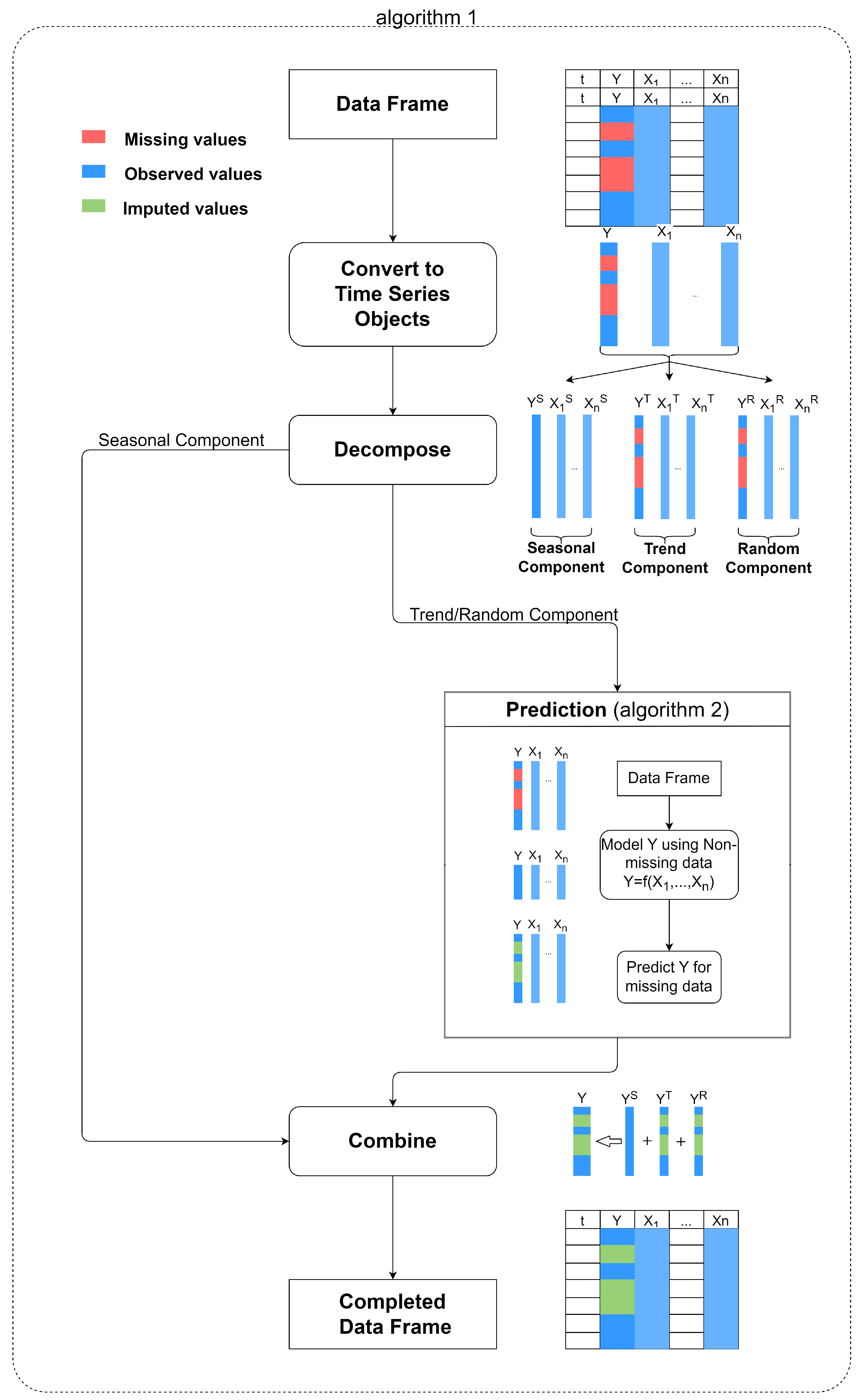
3.4. Proposed Algorithm

The proposed algorithm can be applied to a data set with some specific characteristics. Mainly, there should be one or more correlated time series variables with the time series to be imputed which has large gaps. In air quality data sets, often correlated variables are present. The focus of this algorithm is to impute relatively large gaps.

In this setting, we denote the time series variable to be imputed (with large gaps) as the dependent variable (Y) and the other correlated variables as predictors ($X_1,X_2,\dots ,X_n$). Ideally, the predictors are expected to be complete time series (no missing values) to apply this algorithm. However, this is highly unlikely in real data sets and there may be missing values in almost all the predictors. The first step is to apply well-established univariate imputation methods for each of the predictors and impute missing values when the percentage of missing values is as low as 5%. After this step, if the predictors are complete, then the proposed algorithm can be used. If this is not the case, in Section 5.1, further remedies are proposed. Assuming that the predictors are complete time series, the proposed algorithm can be illustrated as in Figure 2. The main steps of the proposed imputation algorithm can be summarised as follows:

• Decompose all the time series (dependant and predictors) into the seasonal, trend, and random components.
• Leave out the seasonal component and impute missing values in the deseasonalised data based on an elastic net regression model.
• Combine imputed deseasonalised data with the seasonal component and form the complete time series.

Algorithm 1 presents the overall proposed methodology for data imputation and Algorithm 2 presents the elastic net regression-based imputation method.

Algorithm 1 Main Imputation Algorithm

Input: Data frame with time index t, Dependant Y, Predictors $X_1,\dots ,X_n$ 1: $I_{Missing}:\leftarrow indicesofmissingobservationsofY$ 2: $I_{Observed}:\leftarrow indicesofavailableobservationsofY$ 3: Separate the variables ($Y,X_1,\dots ,X_n$) into time series objects 4: Decompose each of the time series objects into Seasonal, Trend, and Random components 5: $Y^S:\leftarrow SeosonalComponentofY$ 6: $Y^T:\leftarrow TrendComponentofY$ 7: $Y^R:\leftarrow RandomComponentofY$ 8: $X^S:\leftarrow SeosonalComponentofPredictors(X_1^S,\dots ,X_n^S)$ 9: $X^T:\leftarrow TrendComponentofPredictors(X_1^T,\dots ,X_n^T)$ 10: $X^R:\leftarrow RandomComponentofPredictors(X_1^R,\dots ,X_n^R)$ 11: Predict the missing values of $Y_T$ using $X_T$ (Algorithm 2) 12: Predict the missing values of $Y_R$ using $X_R$ (Algorithm 2) 13: $Y_{Imputed}\leftarrow Y^S+Y_{completed}^T+Y_{completed}^R$ Output: Complete data frame ($Y_{Imputed},X_1,\dots ,X_n$)

Algorithm 2 Imputing Trend/Random component

Input: Data frame with time index t, Dependant Y, Predictors $X_1,\dots ,X_n$ 1: $D_M\leftarrow Dataframecorrespondingto{I}_{Missing}$ 2: $D_{NM}\leftarrow Dataframecorrespondingto{I}_{Observed}$ 3: procedure PredictiveModel($D_{NM}$) 4:     $TrainData\leftarrow randomsplitof70\%data$ 5:     $TestData\leftarrow restofthe30\%data$ 6:     for each model 1 to N do 7:         Fit the model using TrainData 8:         Predict the output for TestData 9:         Calculate RMSE for TestData 10:     end for 11:     $BestModel\leftarrow modelwithleastRMSE$ 12:     return $BestModel$ 13: end procedure 14: Predict missing Y values in $D_M$ using $BestModel$ Output: Complete Y series ($Y_{completed}^{T}or{Y}_{completed}^R$)

The input for Algorithm 1 is a data frame with a time index (t). First, identify the indices of missing observations of Y. Then, all the variables are converted into separate time series objects which are then decomposed into a seasonal, a trend, and a random component. Seasonal-Trend decomposition procedure based on Loess (STL) [44] can be used for the decomposition of the time series. As it requires a complete series to do the STL decomposition, a simple approximation such as linear approximation can be used to approximate missing values of the Y series. The purpose of this approximation is only to decompose the series and to identify the seasonal component. These approximated values are replaced later with imputed values. Chandrasekaran et al. have also used this procedure to decompose a series with missing values in their Seasonal Moving Window Algorithm (SMWA) for imputing missing values of univariate time series [14]. Generally in decomposition-based forecasting models, the seasonal component is assumed to be unchanging or changing slowly. In most forecasting applications with meteorological variables, seasonally adjusted components are used for the prediction model, and then the output is combined with the seasonal component [45,46,47,48]. The imputation methodology proposed in this paper also uses the seasonally adjusted component for the prediction model. Moreover, the objective of the paper is to impute missing data in a given time series and not forecast. Therefore, once the seasonal component is identified by applying STL decomposition [44] which accounts for the changing seasonality as well, the rest of the components are used for the prediction model. Therefore, in the next step, trend and random components are fed into algorithm 2 while leaving out the seasonal component.

In Algorithm 2, either trend or random components of the dependant (Y) and predictors ($X_1,\dots ,X_n$) with time index are inputted as a data frame. Then, the data frame is divided into two parts based on the time index, one part with complete Y observations and the other part with missing Y observations. The complete data set is further divided into training and testing data sets. The training data set is used to build models to predict Y based on predictors $X_1,\dots ,X_n$ and the testing data set is used to evaluate the models using Root Mean Squared Error (RMSE). Different elastic-net regression models can be used as candidate models (N). In Section 4, three models were used with special cases of elastic net regression models by changing ${\lambda }_1$ and ${\lambda }_2$ parameters.

• Ridge regression with ${\lambda }_1=0$ and ${\lambda }_2>0$
• Lasso regression with ${\lambda }_2=0$ and ${\lambda }_1=>0$
• Elastic net regression with ${\lambda }_1>0$ and ${\lambda }_2>0$

Choosing optimal hyper-parameters and model validation was done using 10-fold cross-validation. The model with the lowest RMSE in the testing data set was used for the prediction (imputation).

3.5. Artificially Generating Missing Data

Performance evaluation of a missing value imputation technique can only be done for simulated missing data. Little and Rubin (2002) present the data structure for simulating missing values in a univariate data set, providing the MCAR mechanism.

Let $Y={(y_1,\dots ,y_n)}^T$ where $y_i$ denotes the value of a random variable for observation i, and let $M={(M_1,\dots ,M_n)}^T$ where $M_i=0$ for units that are observed and $M_i=1$ for units that are missing. Suppose the joint distribution of $f(y_i,M_i)$ is independent across units $i=1,2,\dots ,n$ so that the probability a value is observed does not depend on the values of Y or M for the other units [6].

$$f(Y,M|\theta ,\varphi )=f\left(Y\right|\theta )f\left(M\right|Y,\varphi )=\prod _{i=0}^{n}f\left(y_i\right|\theta )\prod _{i=0}^{n}f\left(M_i\right|y_i,\varphi )$$

(9)

Artificial missing data were simulated under MCAR mechanism using exponential distribution to evaluate the performance of the proposed algorithm. The exponential distribution with rate $\lambda$ has the density

$$f\left(x\right)=\lambda e^{-\lambda x}forx\ge 0.$$

(10)

The simulation procedure is further described in Section 4.

4. Experiments

It is necessary to have a complete data set to evaluate the proposed algorithm. However, it is almost impossible to have a complete data set of this nature. It is important to use a real data set with similar nature to demonstrate the algorithm. After examining daily PM${}_{2.5}$, PM${}_{10}$, and NEPH values for a 20-year period from 2000 to 2020 at 18 selected sites in the Sydney region, a data set from the 2014–2020 period at Earlwood site was selected where the percentages of missing values were equal or below 5%. Kalman smoothing on structural time series models in ImpueTS R package [49] is used to recover the missing values and then the data set is considered as the ground truth. PM${}_{2.5}$ series is selected as the Y series and PM${}_{10}$ and NEPH are used as the predictors. The reason to select PM${}_{2.5}$ as Y is that it consists of large gaps in real data, as investigated in Section 5.1. It is required to artificially create missing values to compare the performance of the proposed algorithm. The simulations are done under the MCAR mechanism using the exponential distribution. Moritz et al. (2015) also used this simulation procedure for their comparison of imputation methods in univariate time series [9]. Five scenarios were created using five different values for the rate parameter of the exponential distribution.

• Scenario1: Missing percentage 10% with rate 0.1
• Scenario2: Missing percentage 20% with rate 0.2
• Scenario3: Missing percentage 30% with rate 0.3
• Scenario4: Missing percentage 40% with rate 0.4
• Scenario5: Missing percentage 50% with rate 0.5

5. Results and Discussion

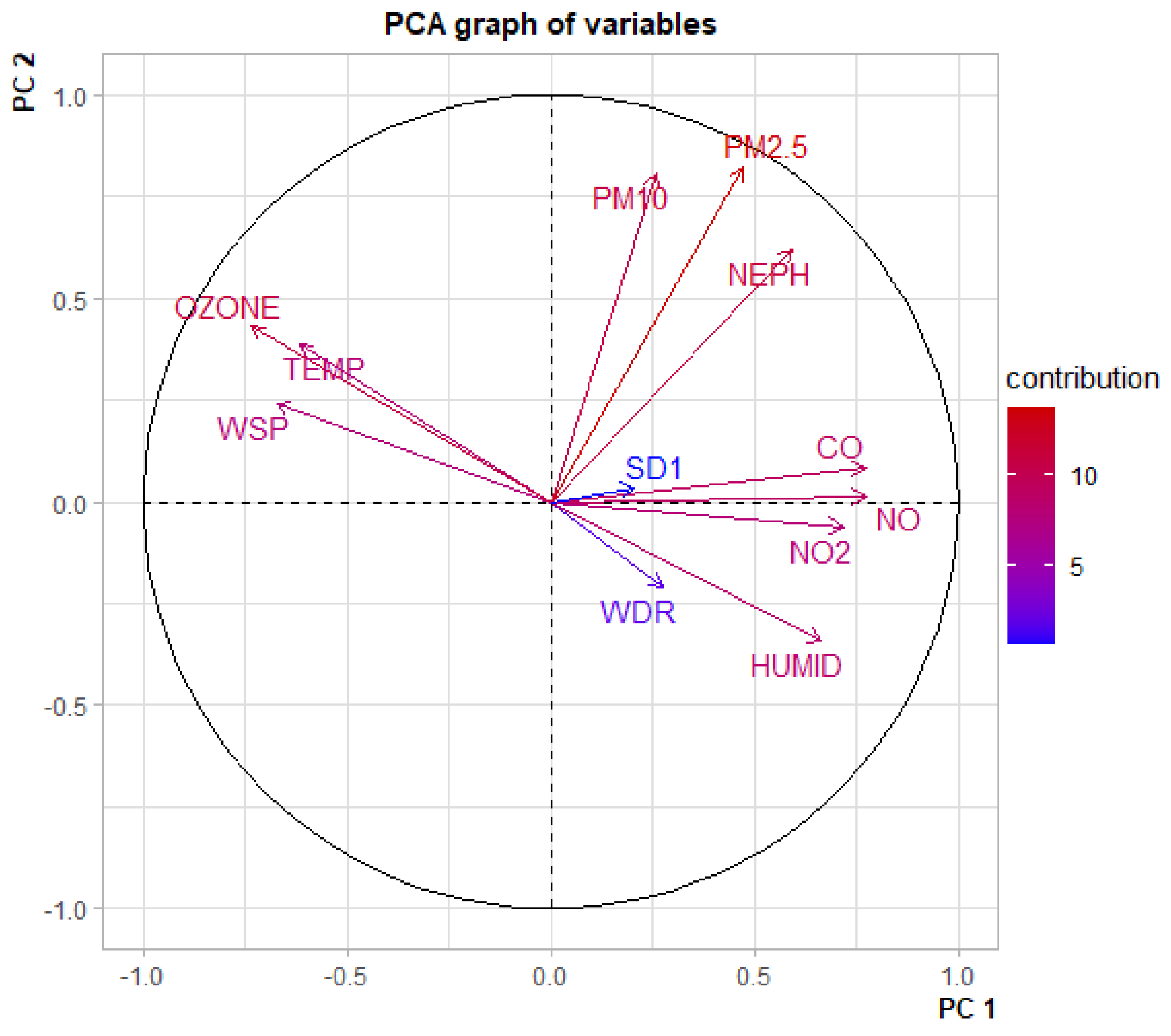
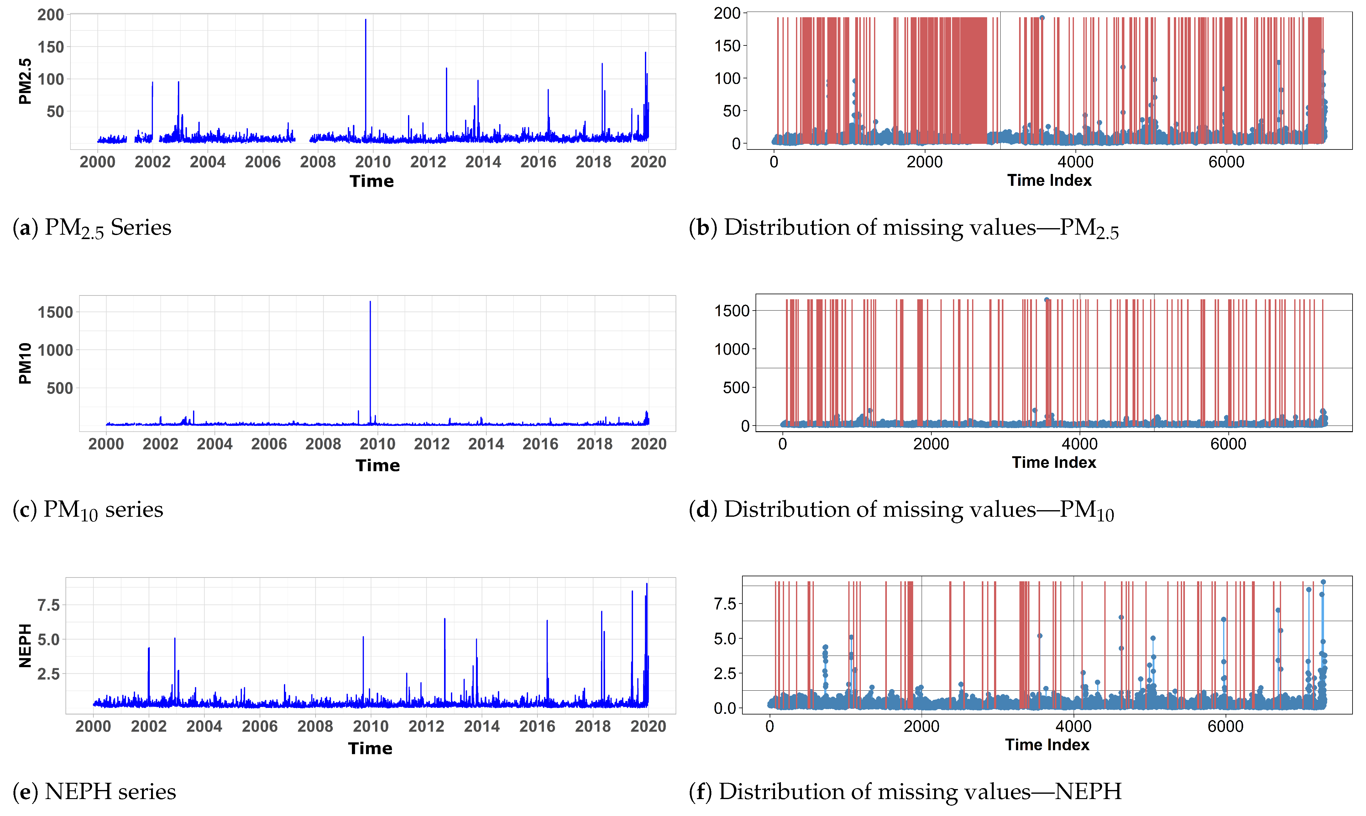
5.1. Exploratory Analysis

Exploratory analysis plays an important role in data-driven solutions. This section presents the results of an exploratory analysis carried out using a meteorology data set. The motivation to propose the methodology presented in this paper arose through this analysis. The considered meteorological data set includes hourly data recorded at the Liverpool monitoring site in the Sydney region, Australia. Principal component analysis (PCA) is an unsupervised technique that can be used to visualize data as well as dimension reduction. To identify the characteristics of the meteorological variables visually, PCA was carried out and the plots were analysed. Figure 3 shows a PCA plot with variables. The variables are shown in arrows while the contribution is represented by colours. The angle between the two arrows reflects the correlation between those two variables.

It can be seen that the following variable sets are highly correlated.

• CO, NO and NO${}_2$ are positively-correlated
• O${}_3$ (Ozone) and Temperature are positively correlated
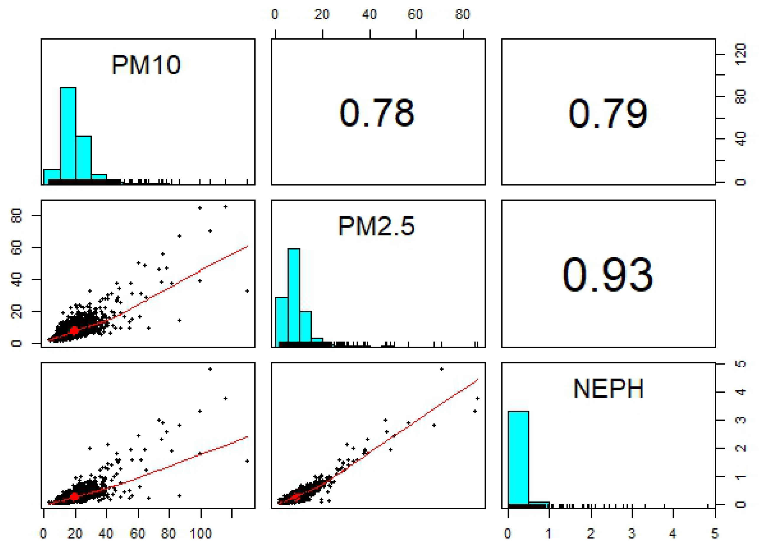
• PM${}_{2.5}$, PM${}_{10}$ and NEPH (a measure of visibility) are positively correlated
• Humidity is negatively correlated with O${}_3$ and Temperature

Similar results can be seen in other monitoring sites in the Sydney region. Therefore the proposed algorithm is particularly applicable to meteorological data sets like this.

Table 2. Missing Statistics of daily PM${}_{2.5}$, PM${}_{10}$ and NEPH observations at three monitoring sites in the Sydney region from 2000 to 2020.

Site	Variable
	PM${}_{2.5}$			PM${}_{10}$			NEPH
	Longest Gap	Frequent Gap	Missing Percent	Longest Gap	Frequent Gap	Missing Percent	Longest Gap	Frequent Gap	Missing Percent
RICHMOND	197	1 NA 179 times	12.4	18	1 NA 63 times	3.85	5	2 NA 28 times	2.07
BRINGELLY	6025	1 NA 11 times	83.1	24	2 NA 15 times	3.48	14	2 NA 31 times	3.01
EARLWOOD	83	1 NA 48 times	5	15	1 NA 41 times	3.29	5	1 NA 14 times	1.77

shows statistics of missing values of daily PM${}_{2.5}$, PM${}_{10}$ and NEPH observations at three selected monitoring sites in the Sydney region from 2000 to 2020.

It can be seen that in PM${}_{10}$ and NEPH, the percentage of missing values is lower than 5% whereas, in PM${}_{2.5}$, the percentage of missing values is relatively very high. Moreover, the longest gap size is also relatively very large for PM${}_{2.5}$ than that of the other two variables. Therefore, existing univariate imputation methods could be used to recover missing values in PM${}_{10}$ and NEPH which could be used as predictors to recover large gaps in PM${}_{2.5}$ (dependent). Figure 4 shows Pearson’s correlation coefficients and scatter plots among the variables. It further clarifies that the variables are highly positively correlated with reasonable positive coefficients. There may be situations where all the variables have percentages greater than 5%. In such situations, a sliding window can be considered such that at least one of the variables has low missing values.

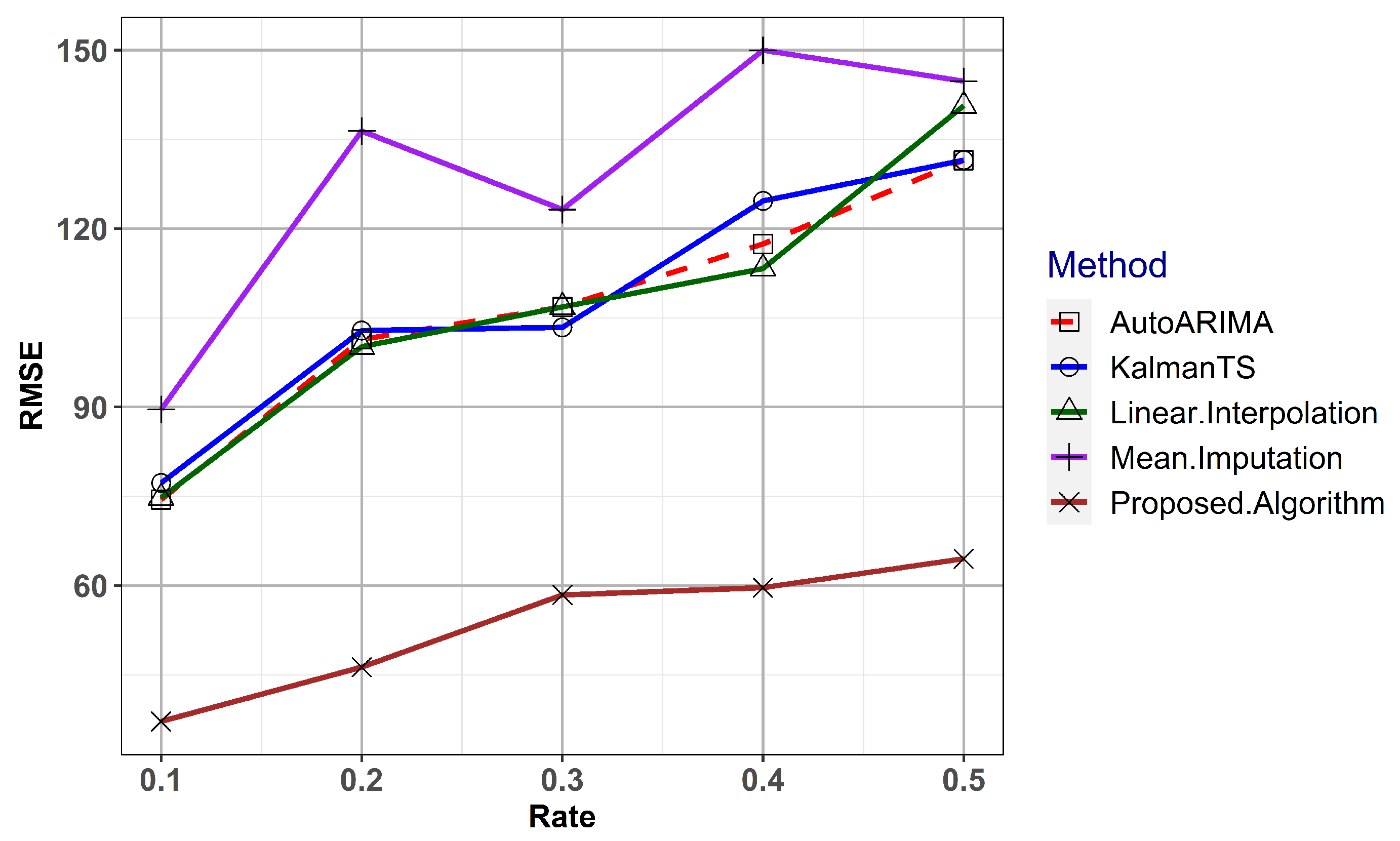
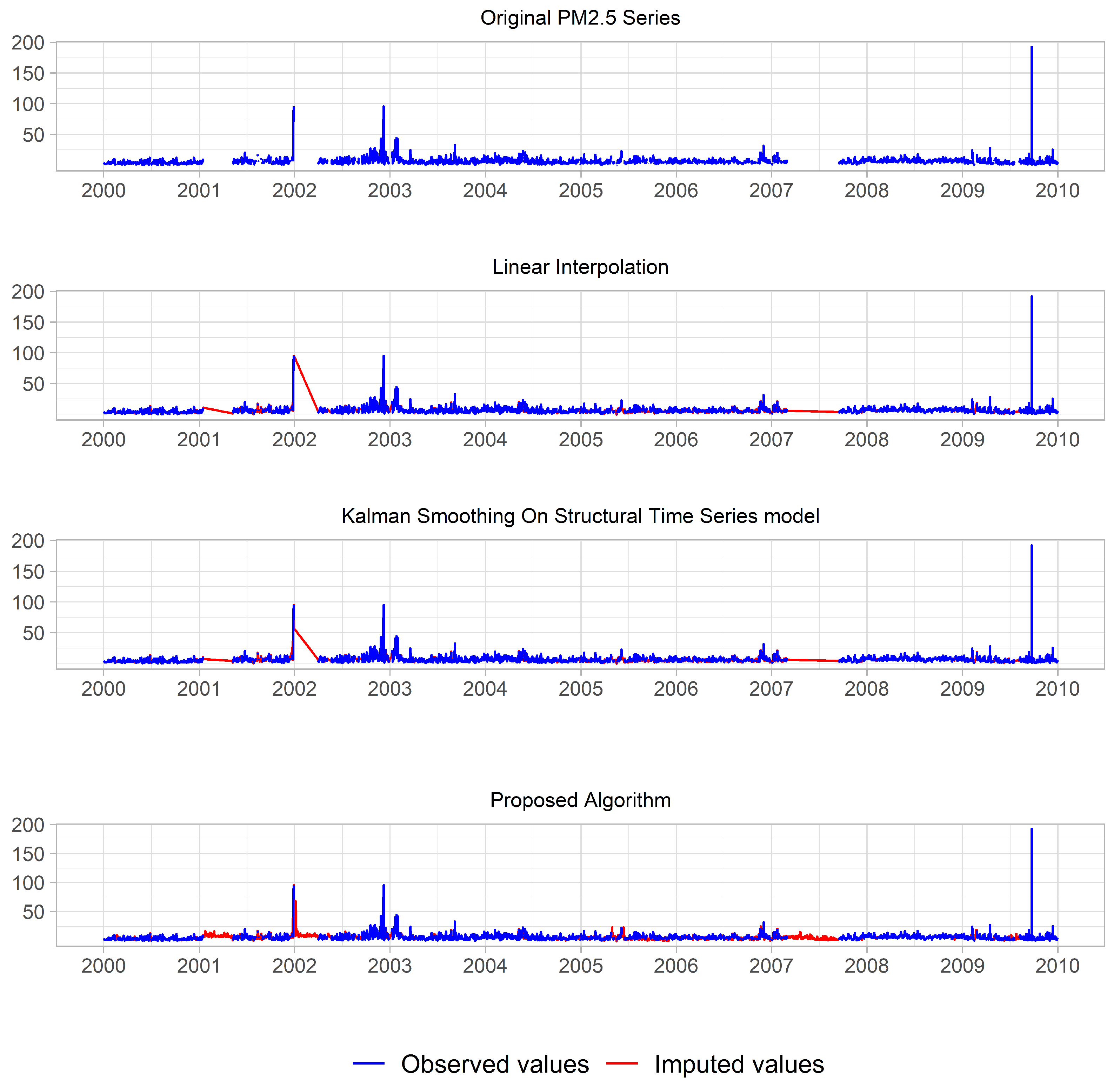
5.2. Performance Evaluation

The proposed algorithm was used to impute the missing values for each of the five different scenarios mentioned in Section 4 and the RMSE was calculated. In order to compare the performance with other existing methods, four well-established methods namely Kalman smoothing on ARIMA models, Kalman smoothing on structural time series models, linear interpolation, and mean imputation were used. Missing values were imputed for the five scenarios using the considered methods. The RMSE values for all the methods in five scenarios are given in Figure 5.

The proposed algorithm has yielded the lowest RMSE for all five scenarios whereas the mean imputation has yielded the largest RMSE values. Linear interpolation and the Kalman smoothing methods perform equally. It is clear that the proposed algorithm outperforms all the other considered methods. The reason is that the proposed algorithm incorporates the information of other correlated variables for the imputation while all the other methods consider only the time series characteristics.

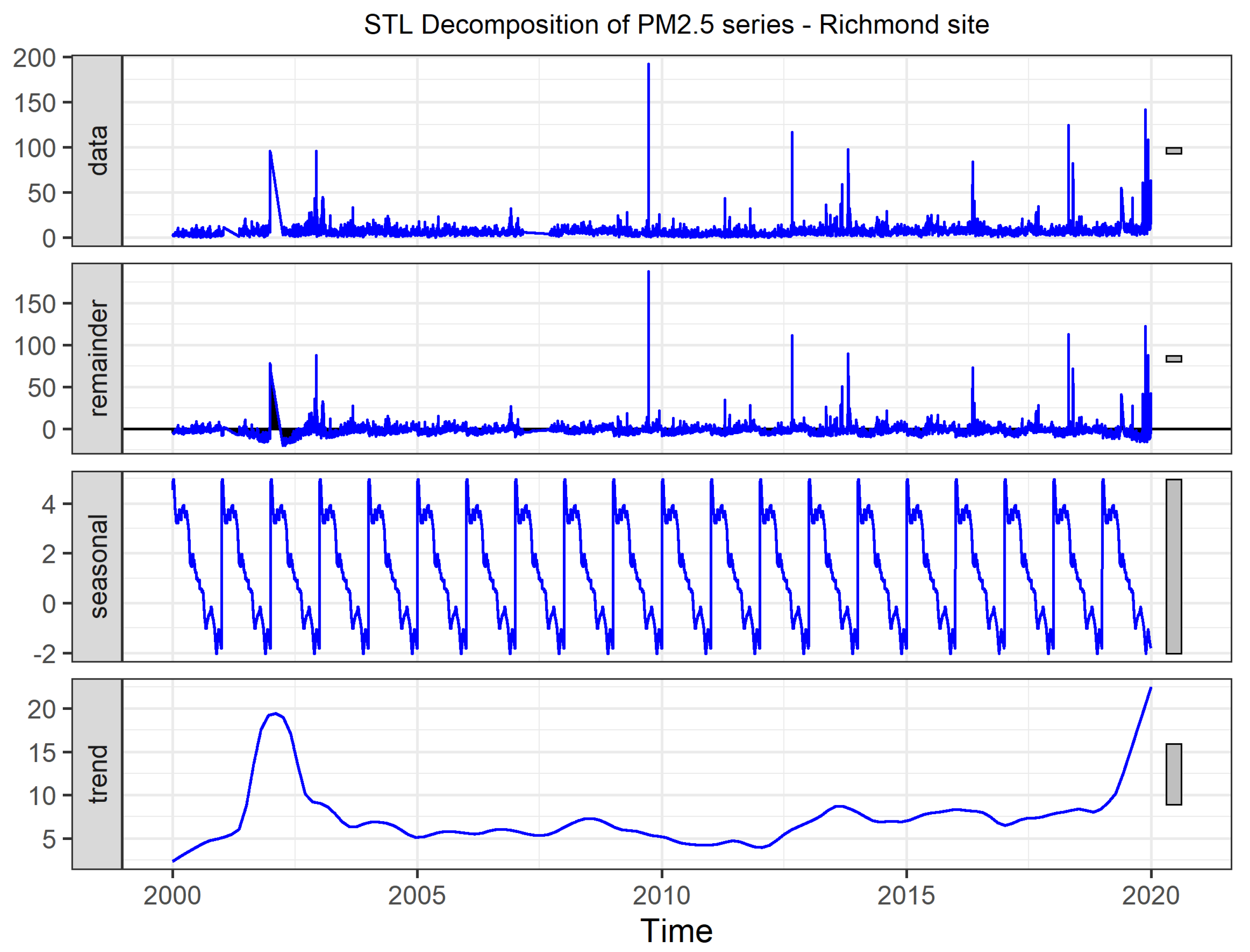
5.3. Real Application

In this Section, the applicability of the algorithm is further demonstrated using a real data set with large gaps. In the data set at the Richmond site, the percentage of missing values in PM${}_{2.5}$ is relatively large (12%) and the longest gap size is 197 days as shown in Table 2. In contrast, PM${}_{10}$ and NEPH have relatively low missing percentages and small gaps. The left-hand side three plots in Figure 6a,c,e show the PM${}_{2.5}$, PM${}_{10}$, and NEPH series from 1 January 2000 to 31 December 2019 and the right-hand side three plots (Figure 6b,d,f) shows the positions of the missing values in each series, highlighting missing regions by red vertical lines. As can be seen, the PM${}_{2.5}$ consists of large gaps while the other two series consist of small gaps.

The proposed algorithm was applied to recover the missing values in PM${}_{2.5}$ series. There is no way to compare the performance in this particular situation as the missing values are actually unknown. However, for a visual comparison, three other methods namely linear interpolation, Kalman smoothing on structural models, and Kalman smoothing on ARIMA models were used to recover the same series and the results were examined. Figure 7 shows the original PM${}_{2.5}$ series with missing values, imputation results of the three other methods, and imputation results of the proposed algorithm. It can be seen that the proposed method has produced more plausible values than the other methods.

6. Conclusions

Missing values are ubiquitous in most real-world scenarios, especially in air quality data sets. Recovery of missing values is an essential part of most of the analyses. Even though there exists a plethora of methods, the performances of those methods depend upon the nature of the data and the missing mechanism. When the percentage of missing values is higher and the gap size is larger, the existing methods perform poorly. The proposed method performs reasonably well in recovering large gaps as it incorporates both the time series characteristics and the information on other correlated variables to recover data. This algorithm can be recommended especially for meteorological data sets with correlated variables to impute large gaps. This method is not applicable in univariate situations.

References

1. Kalivitis, N.; Papatheodorou, S.; Maesano, C.N.; Annesi-Maesano, I. Air quality and health impacts. In Atmospheric Chemistry in the Mediterranean Region; Springer: Berlin/Heidelberg, Germany, 2022; pp. 459–486. [Google Scholar]
2. Hu, W.; Mengersen, K.; McMichael, A.; Tong, S. Temperature, air pollution and total mortality during summers in Sydney, 1994–2004. Int. J. Biometeorol. 2008, 52, 689–696. [Google Scholar] [CrossRef]
3. Ren, C.; Williams, G.M.; Tong, S. Does particulate matter modify the association between temperature and cardiorespiratory diseases? Environ. Health Perspect. 2006, 114, 1690–1696. [Google Scholar] [CrossRef]
4. Simpson, R.; Williams, G.; Petroeschevsky, A.; Best, T.; Morgan, G.; Denison, L.; Hinwood, A.; Neville, G.; Neller, A. The short-term effects of air pollution on daily mortality in four Australian cities. Aust. N. Z. J. Public Health 2005, 29, 205–212. [Google Scholar] [CrossRef]
5. Rubin, D. Inference and missing data. Biometrika 1976, 63, 581–592. [Google Scholar] [CrossRef]
6. Rantou, K. Missing Data in Time Series and Imputation Methods; University of the Aegean: Mytilene, Greece, 2017. [Google Scholar]
7. Rubright, J.D.; Nandakumar, R.; Gluttin, J.J. A simulation study of missing data with multiple missing X’s. Pract. Assess. Res. Eval. 2014, 19, 10. [Google Scholar]
8. Donders, A.R.T.; Van Der Heijden, G.J.; Stijnen, T.; Moons, K.G. A gentle introduction to imputation of missing values. J. Clin. Epidemiol. 2006, 59, 1087–1091. [Google Scholar] [CrossRef]
9. Moritz, S.; Sardá, A.; Bartz-Beielstein, T.; Zaefferer, M.; Stork, J. Comparison of different methods for univariate time series imputation in R. arXiv 2015, arXiv:1510.03924. [Google Scholar]
10. Dixon, W.J. BMDP Statistical Software Manual: To Accompany the… Software Release; University of California Press: Berkeley, CA, USA, 1988. [Google Scholar]
11. Little, R.J. A test of missing completely at random for multivariate data with missing values. J. Am. Stat. Assoc. 1988, 83, 1198–1202. [Google Scholar] [CrossRef]
12. Nakagawa, S. Missing data: Mechanisms, methods and messages. Ecol. Stat. Contemp. Theory Appl. 2015, 81–105. [Google Scholar]
13. Nakagawa, S.; Freckleton, R.P. Missing inaction: The dangers of ignoring missing data. Trends Ecol. Evol. 2008, 23, 592–596. [Google Scholar] [CrossRef]
14. Chandrasekaran, S.; Zaefferer, M.; Moritz, S.; Stork, J.; Friese, M.; Fischbach, A.; Bartz-Beielstein, T. Data Preprocessing: A New Algorithm for Univariate Imputation Designed Specifically for Industrial Needs. In Proceedings of the 26 Workshop Computational Intelligence, Dortmund, Germany, 24–25 November 2016. [Google Scholar]
15. Wijesekara, W.; Liyanage, L. Comparison of Imputation Methods for Missing Values in Air Pollution Data: Case Study on Sydney Air Quality Index. In Proceedings of the Future of Information and Communication Conference, San Francisco, CA, USA, 5–6 March 2020; Springer: Berlin/Heidelberg, Germany, 2020; pp. 257–269. [Google Scholar]
16. Norazian, M.N.; Shukri, Y.A.; Azam, R.N.; Al Bakri, A.M.M. Estimation of missing values in air pollution data using single imputation techniques. ScienceAsia 2008, 34, 341–345. [Google Scholar] [CrossRef]
17. Zakaria, N.A.; Noor, N.M. Imputation methods for filling missing data in urban air pollution data formalaysia. Urban. Arhit. Constr. 2018, 9, 159–166. [Google Scholar]
18. Junger, W.; De Leon, A.P. Imputation of missing data in time series for air pollutants. Atmos. Environ. 2015, 102, 96–104. [Google Scholar] [CrossRef]
19. Junninen, H.; Niska, H.; Tuppurainen, K.; Ruuskanen, J.; Kolehmainen, M. Methods for imputation of missing values in air quality data sets. Atmos. Environ. 2004, 38, 2895–2907. [Google Scholar] [CrossRef]
20. Wijesekara, L.; Liyanage, L. Air quality data pre-processing: A novel algorithm to impute missing values in univariate time series. In Proceedings of the 2021 IEEE 33rd International Conference on Tools with Artificial Intelligence (ICTAI), Virtual, 1–3 November 2021; pp. 996–1001. [Google Scholar]
21. Lei, K.S.; Wan, F. Pre-processing for missing data: A hybrid approach to air pollution prediction in Macau. In Proceedings of the 2010 IEEE International Conference on Automation and Logistics, Hong Kong, China, 16–20 August 2010; IEEE: Piscataway, NJ, USA, 2010; pp. 418–422. [Google Scholar] [CrossRef]
22. Shahbazi, H.; Karimi, S.; Hosseini, V.; Yazgi, D.; Torbatian, S. A novel regression imputation framework for Tehran air pollution monitoring network using outputs from WRF and CAMx models. Atmos. Environ. 2018, 187, 24–33. [Google Scholar] [CrossRef]
23. Che, Z.; Purushotham, S.; Cho, K.; Sontag, D.; Liu, Y. Recurrent neural networks for multivariate time series with missing values. Sci. Rep. 2018, 8, 6085. [Google Scholar] [CrossRef] [PubMed]
24. Yuan, H.; Xu, G.; Yao, Z.; Jia, J.; Zhang, Y. Imputation of missing data in time series for air pollutants using long short-term memory recurrent neural networks. In Proceedings of the 2018 ACM International Joint Conference and 2018 International Symposium on Pervasive and Ubiquitous Computing and Wearable Computers, Singapore, 8–12 October 2018; pp. 1293–1300. [Google Scholar]
25. Lee, M.; An, J.; Lee, Y. Missing-value imputation of continuous missing based on deep imputation network using correlations among multiple iot data streams in a smart space. IEICE Trans. Inf. Syst. 2019, 102, 289–298. [Google Scholar] [CrossRef]
26. Cao, W.; Wang, D.; Li, J.; Zhou, H.; Li, L.; Li, Y. Brits: Bidirectional recurrent imputation for time series. Adv. Neural Inf. Process. Syst. 2018, 31, 1–11. [Google Scholar]
27. Yoon, J.; Zame, W.R.; van der Schaar, M. Estimating missing data in temporal data streams using multi-directional recurrent neural networks. IEEE Trans. Biomed. Eng. 2018, 66, 1477–1490. [Google Scholar] [CrossRef]
28. Luo, Y.; Cai, X.; Zhang, Y.; Xu, J.; Yuan, X. Multivariate time series imputation with generative adversarial networks. Adv. Neural Inf. Process. Syst. 2018, 31, 1–12. [Google Scholar]
29. Luo, Y.; Zhang, Y.; Cai, X.; Yuan, X. E2gan: End-to-end generative adversarial network for multivariate time series imputation. In Proceedings of the 28th International Joint Conference on Artificial Intelligence, Macao, China, 10–16 August 2019; AAAI Press: Palo Alto, CA, USA, 2019; pp. 3094–3100. [Google Scholar]
30. Wu, Z.; Ma, C.; Shi, X.; Wu, L.; Zhang, D.; Tang, Y.; Stojmenovic, M. BRNN-GAN: Generative Adversarial Networks with Bi-directional Recurrent Neural Networks for Multivariate Time Series Imputation. In Proceedings of the 2021 IEEE 27th International Conference on Parallel and Distributed Systems (ICPADS), Beijing, China, 14–16 December 2021; IEEE: Piscataway, NJ, USA, 2021; pp. 217–224. [Google Scholar]
31. Miao, X.; Wu, Y.; Wang, J.; Gao, Y.; Mao, X.; Yin, J. Generative semi-supervised learning for multivariate time series imputation. In Proceedings of the AAAI Conference on Artificial Intelligence, Virtual, 2–9 February 2021; Volume 35, pp. 8983–8991. [Google Scholar]
32. Liu, Y.; Yu, R.; Zheng, S.; Zhan, E.; Yue, Y. Naomi: Non-autoregressive multiresolution sequence imputation. Adv. Neural Inf. Process. Syst. 2019, 32, 1–11. [Google Scholar]
33. Khayati, M.; Lerner, A.; Tymchenko, Z.; Cudré-Mauroux, P. Mind the gap: An experimental evaluation of imputation of missing values techniques in time series. In Proceedings of the VLDB Endowment, Online, 31 August–4 September 2020; Volume 13, pp. 768–782. [Google Scholar]
34. Troyanskaya, O.; Cantor, M.; Sherlock, G.; Brown, P.; Hastie, T.; Tibshirani, R.; Botstein, D.; Altman, R.B. Missing value estimation methods for DNA microarrays. Bioinformatics 2001, 17, 520–525. [Google Scholar] [CrossRef] [PubMed]
35. Mazumder, R.; Hastie, T.; Tibshirani, R. Spectral regularization algorithms for learning large incomplete matrices. J. Mach. Learn. Res. 2010, 11, 2287–2322. [Google Scholar] [PubMed]
36. Cai, J.F.; Candès, E.J.; Shen, Z. A singular value thresholding algorithm for matrix completion. SIAM J. Optim. 2010, 20, 1956–1982. [Google Scholar] [CrossRef]
37. Khayati, M.; Böhlen, M.; Gamper, J. Memory-efficient centroid decomposition for long time series. In Proceedings of the 2014 IEEE 30th International Conference on Data Engineering, Chicago, IL, USA, 31 March–4 April 2014; IEEE: Piscataway, NJ, USA, 2014; pp. 100–111. [Google Scholar]
38. Khayati, M.; Cudré-Mauroux, P.; Böhlen, M.H. Scalable recovery of missing blocks in time series with high and low cross-correlations. Knowl. Inf. Syst. 2020, 62, 2257–2280. [Google Scholar] [CrossRef]
39. Balzano, L.; Chi, Y.; Lu, Y.M. Streaming pca and subspace tracking: The missing data case. Proc. IEEE 2018, 106, 1293–1310. [Google Scholar] [CrossRef]
40. Zhang, D.; Balzano, L. Global convergence of a grassmannian gradient descent algorithm for subspace estimation. In Proceedings of the Artificial Intelligence and Statistics, Cadiz, Spain, 9–11 May 2016; PMLR: London, UK, 2016; pp. 1460–1468. [Google Scholar]
41. Wellenzohn, K.; Böhlen, M.H.; Dignös, A.; Gamper, J.; Mitterer, H. Continuous imputation of missing values in streams of pattern-determining time series. In Proceedings of the 20th International Conference on Extending Database Technology (EDBT 2017), Venice, Italy, 21–24 March 2017. [Google Scholar]
42. Ruan, W.; Xu, P.; Sheng, Q.Z.; Tran, N.K.; Falkner, N.J.; Li, X.; Zhang, W.E. When sensor meets tensor: Filling missing sensor values through a tensor approach. In Proceedings of the 25th ACM International on Conference on Information and Knowledge Management, Indianapolis, IN, USA, 24–28 October 2016; pp. 2025–2028. [Google Scholar]
43. Jerrett, M.; Arain, A.; Kanaroglou, P.; Beckerman, B.; Potoglou, D.; Sahsuvaroglu, T.; Morrison, J.; Giovis, C. A review and evaluation of intraurban air pollution exposure models. J. Expo. Sci. Environ. Epidemiol. 2005, 15, 185–204. [Google Scholar] [CrossRef]
44. Cleveland, R.B.; Cleveland, W.S.; McRae, J.E.; Terpenning, I. STL: A seasonal-trend decomposition. J. Off. Stat. 1990, 6, 3–73. [Google Scholar]
45. Zhang, W.; Wang, J.; Wang, J.; Zhao, Z.; Tian, M. Short-term wind speed forecasting based on a hybrid model. Appl. Soft Comput. 2013, 13, 3225–3233. [Google Scholar] [CrossRef]
46. Wang, J.; Zhang, W.; Wang, J.; Han, T.; Kong, L. A novel hybrid approach for wind speed prediction. Inf. Sci. 2014, 273, 304–318. [Google Scholar] [CrossRef]
47. Wang, J.; Qin, S.; Zhou, Q.; Jiang, H. Medium-term wind speeds forecasting utilizing hybrid models for three different sites in Xinjiang, China. Renew. Energy 2015, 76, 91–101. [Google Scholar] [CrossRef]
48. Prema, V.; Rao, K.U. Time series decomposition model for accurate wind speed forecast. Renew. Wind Water Sol. 2015, 2, 1–11. [Google Scholar] [CrossRef]
49. Moritz, S.; Bartz-Beielstein, T. imputeTS: Time series missing value imputation in R. R J. 2017, 9, 207. [Google Scholar] [CrossRef]
Figure 1. Decomposition of a time series into trend, seasonal, and remainder components: Top panel shows the original time series. The second panel shows the remainder. The third panel shows the seasonal component. Bottom panel shows the trend component.
Atmosphere 14 00355 g001
Figure 2. Schematic representation of the proposed algorithm.
Atmosphere 14 00355 g002
Figure 3. Principal Component Analysis plot of variables.
Atmosphere 14 00355 g003
Figure 4. Scatter Plot of Matrices (SPLOM) of PM 10 , PM 2.5 and NEPH. Pearson Correlation Coefficients above the diagonal, histograms on the diagonal, and bivariate scatter plots below the diagonal. Red lines represent the linear regression fits.
Atmosphere 14 00355 g004
Figure 5. Performance Comparison of the Proposed method against Kalman smoothing on ARIMA models, Kalman smoothing on structural time series models, Linear interpolation, and Mean imputation.
Atmosphere 14 00355 g005
Figure 6. Distribution of missing values of the variables PM 2.5 , PM 10 , and NEPH: Left-hand figures (a,c,e) show the original time series whereas Right-hand figures (b,d,f) show the distribution of missing values with red lines representing the positions of missing values and blue lines representing the original series.
Atmosphere 14 00355 g006
Figure 7. Visual comparison of the imputed values for a large gap using Linear interpolation, Kalman Smoothing On Structural Time Series model and the proposed algorithm.
Atmosphere 14 00355 g007