Article

Modeling and Assessment of PM10 and Atmospheric Metal Pollution in Kayseri Province, Turkey

1
Department of Environmental Engineering, Necmettin Erbakan University, 42090 Konya, Turkey
2
Department of Environmental Engineering, Engineering and Natural Science Faculty, Konya Technical University, 42250 Konya, Turkey
3
South Central Anatolia Clean Air Directorate, 42080 Konya, Turkey
*
Author to whom correspondence should be addressed.
Atmosphere 2023, 14(2), 356; https://doi.org/10.3390/atmos14020356
Submission received: 23 December 2022 / Revised: 3 February 2023 / Accepted: 7 February 2023 / Published: 10 February 2023

Abstract

:
Air pollution has numerous detrimental consequences for human health, visibility, climate, materials, plant health, and animal health. A portion of air pollution consists of metals, which are emitted into the environment via the combustion of fossil fuels, industrial activities, and the incineration of metal-containing products. In this work, the particulate matter and particle-related metal pollution from various sources, in the Turkish province of Kayseri, were determined. AERMOD modeling was also used to examine the distribution of PM10 around the Kayseri Organized Industrial Zone (OIZ). Particulate matter (PM10) samples were collected using MCZ dust collecting devices at six monitoring locations mainly affected by residential heating (Hürriyet, Talas, and Kocasinan), industry (OIZ), and traffic (Tramway and Cumhuriyet) during the autumn/winter months and at three monitoring locations mainly affected by residential heating (Kocasinan), industry (OIZ), and traffic (Tramvay) during the spring months. ICP-MS analysis was used to assess the concentrations of the heavy metals (Pb, As, Cd, and Ni) in samples collected over 6 different time periods of 16 days each. During the autumn/winter months, the concentrations of Pb near roadways were found to exceed the Air Quality Assessment and Management Regulation of Turkey (AQAMR) limit value. During all the sampling periods, the Ni and Cd concentrations were below the AQAMR limit values. At the points associated with winter heating, the concentrations exceeded the AQAMR limit value, which may result from coal combustion.

1. Introduction

Air pollution is one of the biggest threats to our world. It is bad for all living things, the climate, and buildings and structures. Parallel to the rapid increase in the world population in the 21st century, air pollution has become a worldwide problem because of increasing energy use, industrial development, and urbanization [1]. To improve air quality, it is necessary to identify and apportion the emission sources and to determine and implement the most effective pollution control strategies [2]. Pollutants exist in the air in gaseous, liquid, or solid form. They are classified into two groups: natural and anthropogenic. In addition to primary pollutants, which are directly emitted to the atmosphere by emission sources, secondary pollutants, formed by photochemical reactions of these pollutants in the atmosphere, are also important for urban air quality [3]. Primary pollutants include sulfur dioxide (SO2), nitrogen oxides (NOx), carbon monoxide (CO), carbon dioxide (CO2), and particulate matter (PM), although particulate matter can also be a secondary pollutant [4,5,6]. Moreover, the impact of organic pollutants, such as hydrocarbons and polycyclic aromatic hydrocarbons (PAHs), on air quality and human health is considerable [7,8].
Particulate matter (PM) is defined as a suspension formed by the fine solid or liquid substances in a gas, which arises from natural sources, such as the soil, the sea, and volcanoes, or from anthropogenic activities and is generally referred to as aerosol in the literature [9]. Particle sizes in atmospheric PM can vary greatly. PM10 and PM2.5 represent mass concentrations of particles with an aerodynamic diameter equal to or less than 10 and 2.5 μm, respectively. PM2.5 can remain in the atmosphere for weeks or months; PM10 can precipitate out of the atmosphere within a few hours [10]. PM has a high potential for adsorbing toxic metals, creating serious health problems [11]. Metal concentrations in PM of 30–35 μg/m3 were reported in the literature [6,12]. Manganese, copper, zinc, cadmium, chromium, iron, nickel, potassium, calcium, vanadium, barium, arsenic, selenium, and strontium are the most commonly found metals and metalloids in the pollution sources and have been studied widely. In Western Europe, North America, and the western Pacific, except for China, the annual mean total suspended particulate (TSP) concentrations range between 20 and 80 µg/m3 [12,13], and PM10 levels are between 10 and 55 µg/m3. High TSP and PM10 annual mean concentrations are found in Southeast Asia [12,13]. Epidemiological studies have discovered a link between PM pollution levels and deaths from cardiovascular and respiratory diseases [14]. All metals that cause environmental pollution and have toxic effects are called “heavy metals”. This group consists of more than 60 metals, including lead (Pb), cadmium (Cd), chromium (Cr), iron (Fe), cobalt (Co), copper (Cu), nickel (Ni), mercury (Hg), and zinc (Zn). Heavy metals have cumulative effects and, even in concentrations below the limit values, can have an impact on human health and the environment, in the medium–long term [15]. The most important industrial activities that affect the release of heavy metals into the environment are cement production, the iron and steel industry, thermal power plants, glass production, garbage disposal, and waste sludge incineration plants [16]. Heavy metals emitted into the air eventually reach the soil as well as, from there, animals and plants, before moving through the food chain to reach humans. They are also inhaled by animals and humans as airborne aerosols. Heavy metals also reach animals and humans through the contamination of drinking water by industrial wastewaters or contaminated particles involved in pollination [17,18]. Therefore, it is significantly important to monitor the heavy metals found in particulate matter to identify pollution sources and take preventive precautions.
Air quality distribution models are based on the calculation of the dispersion of the pollutant from a source to the receptor points in the impact area, under different atmospheric conditions, using mathematical techniques. These models are generally used in order to predict the possible pollution impact of the industrial facilities and to take preventive measures. The Environmental Protection Agency (EPA)’s AERMOD model is one of these models, and its data flow is provided in Figure S1 [19]. When it comes to predicting pollution concentrations, AERMOD has gained worldwide acceptance, particularly in industrialized nations [20]. The AERMOD modeling system is suggested for field impacts up to 50 km from a site (the emission source) [21]. There are several studies exploring the impacts of the dispersion of air pollutants in different types of areas. For example, in a study performed in the USA, the modeled hourly PM concentration was close to the measured PM concentrations downwind of the source [22]. In another study conducted in Pennsylvania, USA, by including planetary boundary layer turbulence and terrain effects, AERMOD could better predict how pollutants behave near their sources [23]. Moreover, the findings of a study carried out in Iran demonstrated consistent PM10 dispersion in all directions, which was to be expected given the flat modeling region. The simulated maximum PM10 concentrations were higher than the maximum threshold in the guidelines for a 24 h period [24].
In this study, PM10 was sampled during 12 periods of the autumn/winter and spring seasons in six monitoring locations (each mainly affected by residential heating, industry, or traffic emissions), in the Turkish province of Kayseri. Moreover, the metal content of these samples was analyzed according to the TS EN 14902:2006 Ambient Air Quality-Standard Method, and the results were evaluated with respect to Directive 2008/50/EC and the Air Quality Assessment and Management Regulation of Turkey (AQAMR) annual limit values. Moreover, an AERMOD modeling study was conducted to determine the distribution of PM10 pollution in the study area, according to two different scenarios.

2. Materials and Methods
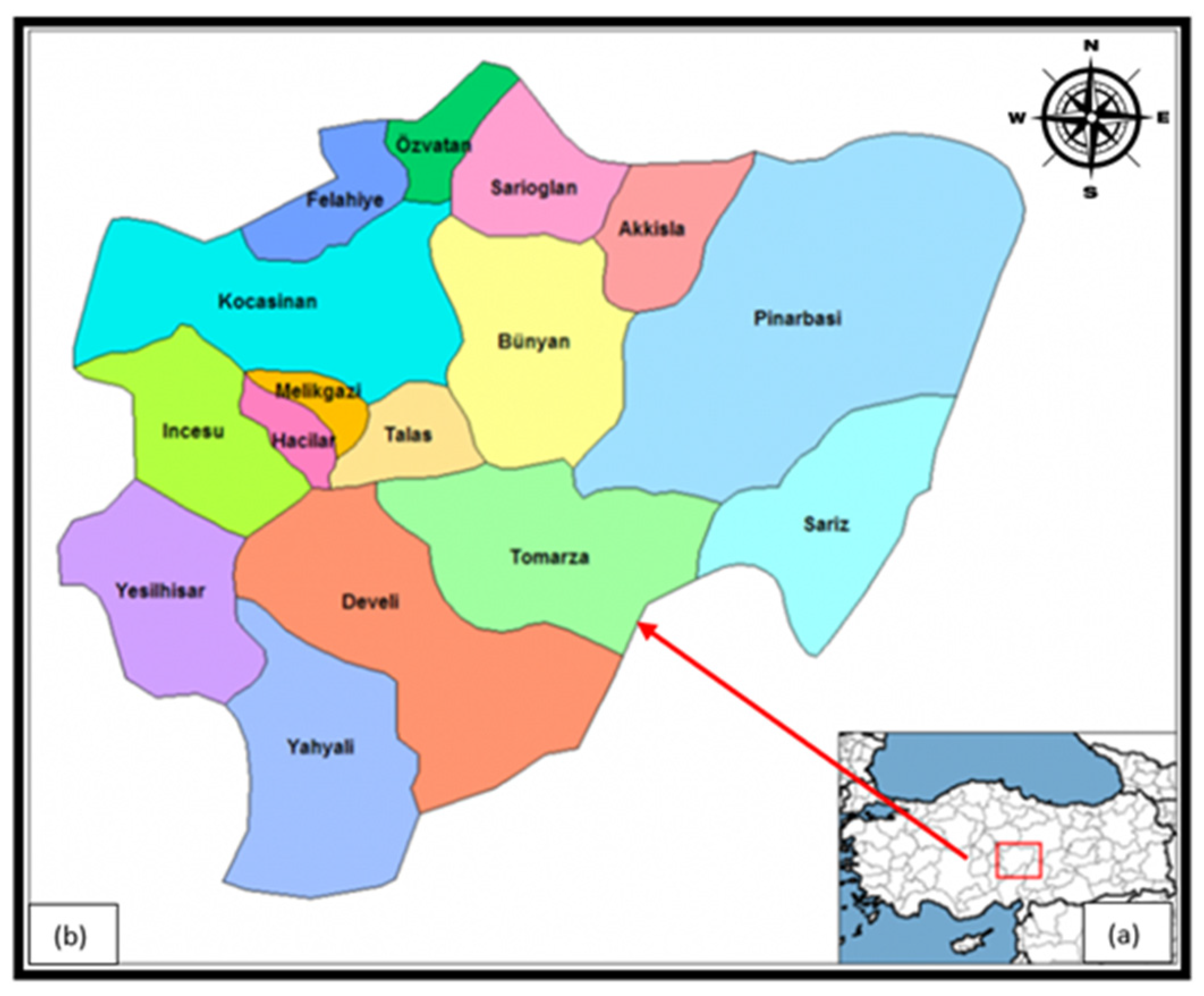
2.1. Study Area

Kayseri is in the upper Kızılırmak portion of Central Anatolia, where the southern section and the Taurus Mountains meet. It is surrounded by Sivas to the east and northeast, Yozgat to the north, Nevşehir to the west, Niğde to the southwest, and Adana and Kahramanmaraş to the south. The province of Kayseri, which is located between 34°56′–36°59′ E longitudes and 37°45′–38°18′ N latitudes, covers 2.2% of the country’s territory, with an area of 16,917 km2. The altitude of the city center is 1054 m above sea level [25].
Approximately 40% of the provincial area is agricultural land. Forest and heathland occupy the lowest ratio of land use [25]. The province has 16 districts, together with a central district. The map of Turkey and Kayseri Province is presented in Figure 1.
The provincial population growth between 2009–2019 was 16.7%, and, according to the Turkish Statistical Institution’s 2023 projection, the population is predicted to increase [27]. Kayseri is a province with developed industry, transportation, and energy infrastructures and rich underground resources. Kayseri, which has 3 Organized Industrial Zones (OIZs), 16 Industrial Sites, 1 Free Zone, and 1 Technology Development Zone, is a production leader in many sectors. There are significant investments in the fields of textiles, apparel, knitting, cleaning materials, electrical and communication products, agricultural tools and machinery, and defense as well as automotive industry in Kayseri.
The wind rose, prepared from the data of Kayseri Meteorology Station No. 17196, during the 1960–2015 period, is presented in Figure S2. According to this wind rose, the 1st degree prevailing wind direction was south, and the 2nd degree prevailing wind direction was west–northwest.
According to the hourly measurements performed by Kayseri Meteorology Station no. 17196, between 1 January 2019 and 31 December 2019, the annual average temperature measured in Kayseri was 11.9 °C. The highest monthly average temperature was 22.3 °C, in August, and the lowest monthly average temperature was −0.7 °C, in January. In Figure 2, the wind rose, prepared from the 2014 data of Kayseri Meteorology Station No. 17195, is presented, showing that the prevailing wind direction was west–southwest and east–northeast. The annual average wind speed was 3.0 m/s, and the daily maximum wind speed was 4.8 m/s.

2.2. Sampling Periods and Location of Six Sampling Points

Sampling was performed at six points: Organized Industrial Zone (OIZ), Hürriyet, Talas, Kocasinan, Tramvay, and Cumhuriyet (Figure 2). The coordinates of the sampling points, main pollution source type, and sampling schedule are presented in Table 1. The sampling points were selected with respect to the predominance of different pollution source types (industry, residential heating, and traffic), according to the characteristics of the respective areas.

2.3. Sampling Method

MCZ PM10 Sampler and PTFE membrane disc filters (47 mm in diameter) were used in the study. MCZ—Model LVS1—Low Volume Dust Sampler is a microcomputer-controlled device, and it performs sampling automatically. The gas flow is physically corrected by pressure and temperature compensation and is evaluated as a correction variable by the electronic control unit. The system is controlled by the control module (MicroPNS). A PM10 sampling head was used, with 2.3 m3/h flow rate, for a 24 h filter sampling duration [29]. In each sampling period, 16 daily samples were collected (corresponding to the capacity of the device), and samples were analyzed.
The sampler was placed in the field, in accordance with the instructions of the manufacturer, with special attention paid to the siting specifications [30]. The calibrated flowmeter was used by performing a leak test and verifying the sampler’s flow rate at least once every three months, in accordance with the instructions of the manufacturer. If the flow rate deviated by more than 5% from its nominal value, the sampler was calibrated by adjusting the flow rate. Periodic filter blanks at each sampling point were taken (at least once for every 20 filters used). In the filter log, the complete information about each sample was recorded, including the stop time, the flow rate, the sample air volume (in m3), any mechanical or electrical failures, the meteorological conditions during the sampling period, and any other information that may be relevant to a later evaluation of the sampling. The inlet impaction plate was cleaned and lubricated at least once every 15 days of sampling. In accordance with the recommendation of the manufacturer, the PM10 sample head was cleaned at least once every six months [30].

2.4. Chemical Analysis

Inductively coupled plasma mass spectrometry (ICP-MS) was used in the heavy metal analysis, and TS EN 14902:2006 Ambient Air Quality-Standard Method was applied for the measurement of Pb, Cd, As, and Ni in the PM10 fraction of suspended particulate matter, by the Environmental Reference Laboratory of Ministry of Environment and Urbanization, accredited by the Turkish Accreditation Agency (TÜRKAK) with the number AB-0262-T.

2.4.1. Pre-Treatment Procedure

The pre-treatment procedure was conducted at the Clean Air Center Directorate Laboratory of the Ministry of Environment and Urbanization.
Microwave dissolution process [30] (CEM MARS-6): In the pre-processing laboratory, filters were conditioned, and the particulate material on the filters was taken to the liquid phase using 10 mL mixture of HNO3 (10.8 M) and HCl (3.0 M).
Microwave fractionation program: The fractionation process was conducted with an 800 W microwave device. The device rose to 190 °C in 20 min and completed its program by waiting 25 min at this temperature.
The sample extracts were stored in the refrigerator and delivered to the Environment Reference Laboratory of Ministry of Environment and Urbanization by cold chain.

2.4.2. ICP-MS Analysis

For ICP-MS analysis, a Bruker Aurora M90 ICP-MS device was used. The samples taken into the liquid phase were transferred to plastic centrifuge tubes and were completed to 25 mL with ultrapure water. The samples were centrifuged at 3000 rpm for 15 min, and the filter residues were precipitated. An aliquot of 2 mL was adjusted up to 10 mL with ultrapure water, and 100 µL of internal standard at 500 µg/L concentration was added and analyzed in the ICP-MS device.
Quality control for ICP-MS device: After calibration, quality control solutions were created independently from the calibration solutions and analyzed to monitor the performance of the method.

2.5. PM10 Determination

Filters were weighed before and after sampling, and PM10 mass concentrations were determined according to the following equation:
PM 10   ( μ g / m 3 ) = B A * 10 6 Q * t
  • A = weighing before sampling (g);
  • B = weighing after sampling (g);
  • Q = flow rate (m3/h);
  • t = sampling period (24 h).
 Equation (2) was used for calculation of the metal concentrations in the sample.
Metal   concentration   ( μ g / m 3 ) = μ g filter Q   m 3 h * 1 / 24

2.6. Inversion Intensity

Under normal weather conditions, temperature tends to drop between 0.5 and 1.0 °C per 100 m of altitude [31]. “A temperature inversion” occurs when the temperature increases rather than decreases with height. If the inversion begins at or near the ground, vertical movements are negligible, water vapor and atmospheric pollutants are unable to rise, there is no horizontal transport, and, as a result, pollutant concentrations in the atmosphere increase, and an air pollution problem may occur [31]. The severity, duration, thickness, and height of the inversion directly affect the intensity of the air pollution experienced. The General Directorate of Meteorology determines inversion intensity for the risk of air pollution in city centers and some district centers, particularly in winter, to notify the public and ensure that the necessary measures are taken by the relevant institutions. The inversion intensity data were provided by the directorate [31].

2.7. AERMOD Model

AERMOD 9.6.0 model version [32] was used to determine the level of PM10 contribution of the industries in the OIZ. To create a model in AERMOD, the following steps are conducted (Figure S1 in the Supplementary Materials):
  • Output type (concentration, dry–wet precipitation, etc.), average time option, dispersion coefficient, and terrain options are entered into the model.
  • Contaminant type is selected, and pollutant sources are entered into the model. If the calculation is to be made for an urban area, the population value is inserted. Variable emissions, if any, are defined.
  • Receptor points are identified by cartesian or polar coordinates.
  • Meteorology files compiled by AERMET View or RAMMET View are entered into the model. The time interval to be modeled is selected (Table S4).
  • The desired output types are selected.
  • After the sources and receptor points are entered into the model, the AERMAP model is run.
  • Finally, the air quality model is run.
In the modeling, the contribution value to the 24 h average PM concentration is taken as the output. Seven hundred twenty receptors were considered in the model, and a distribution with a radius of approximately 11 km (uniform polar grid) was chosen. The meteorological and synoptic data used in modeling were obtained from the closest Erkilet Airport Meteorology Station (No. 17195). Two scenarios were created in the modeling program. The source points considered in these scenarios and their activity sectors are presented in Table S1 (Supplementary Materials).
Scenario 1: The pollutants of 18 facilities with high polluting impact within the scope of Annex-1 of the Environmental Permit and License Regulation, located in Kayseri OIZ and Kayseri Free Zone, were taken into consideration. All plants, except Erbosan, were selected from the plants with the highest pollution impact in the industrial area. In modeling, it was assumed that the total population affected by these facilities is 150,000 inhabitants. It was stated in the model that the facilities operate during all months of the year and at all hours of the day.
Scenario 2: Outside the OIZ and Kayseri Free Zone, 2 facilities with emissions of pollutants included in Annex-1 of the Environmental Permit and License Regulation, were taken into consideration. In this scenario, Kayseri sugar and zinc plants, which use high amounts of coal in their processes, were taken into account, outside the industrial zone. The model was run by stating that while the zinc facility works all days of the year, the sugar facility operates seasonally, in November, December, and January.

3. Results and Discussion

3.1. PM10 Concentrations and Inversion Intensity

The PM10 concentrations were compared with the daily limit value of 50 μg/m3, established by the Air Quality Assessment and Management Regulation (AQAMR, published in the Official Gazette on 6 June 2008, No. 26898) and in the EU Directive 2008/50/EC of 21 May 2008. The PM10 concentrations were also compared with the WHO daily guideline value of 45 μg/m3, which must not be exceeded more than 3–4 days per year [33].
The daily average concentration values at the sampling points for the autumn/winter and spring periods are compared in Figure 3. Daily average PM10 concentrations higher than the EU Directive daily limit (50 μg/m3) were observed in the autumn/winter period, for all locations. In each of the sampling points, the WHO daily guideline value was exceeded on 8 or more days, in the autumn/winter sampling periods (Figure 3). The highest PM10 concentrations were observed at the Hürriyet sampling point. The main pollution source type at this point is residential heating, so the results found may originate from combustion processes. Moreover, the results observed at the OIZ and Tramvay sampling points show that industry and traffic significantly contribute to PM10 pollution in the autumn/winter period. In the spring period, the PM10 concentrations were similar in the various locations and were below the EU Directive daily limit, but the WHO daily guideline value (45 μg/m3) was exceeded on 4 or more days at each location, especially at the OIZ. The average concentration observed at the OIZ (93.2 μg/m3) in the autumn/winter period is high, when compared with similar studies conducted around industrial facilities in different countries. For example, the following average daily PM10 concentrations were observed: 44.4 µg/m3 in Capana, Argentina [34]; 33.3 µg/m3 in Onda, Spain [35]; 54.9 µg/m3 in Elefsina, Greece [36]; and 76.0 µg/m3 in Pohang industrial area, Korea [37]. However, much higher average PM10 concentrations (169 µg/m3) were detected in the industrial area of Rio de Janeiro, Brazil [38].
The daily PM10 concentrations and inversion intensity values, for the autumn/winter and spring periods, are presented in Figure 4 and Figure 5, respectively.
The results indicate that, for the autumn/winter period, there is a weak or very weak correlation between inversion intensity and PM10 concentration at the sampling points for which the main pollution sources are residential heating and traffic, while, at the OIZ sampling point, a strong correlation was found. The OIZ is the only sampling point where industrial emissions predominate. The main reason for this difference might be the emissions from the stacks of the facilities, because the pollutants are emitted from higher heights. The correlation is positive (r = 0.718), indicating that higher PM10 concentrations were registered for higher inversion intensities, as expected. In fact, PM typically shows higher levels during the cold season, due to the lower mixing layer heights and stagnant episodes associated with thermal inversion [39].
The correlation coefficient (r) was determined for each sampling location (Table 2).

3.2. PM10 Metal Concentrations

The daily average metal concentrations for autumn/winter and spring periods are presented in Table 3. The concentrations of 18 metals and 3 metalloids in PM10 were analyzed at the sampling points. The major elements were Al, Fe, Mg, K, Na, and Ca.
The concentration of Al was higher at the OIZ sampling point, which is mainly affected by industry, which can be due to the emissions of the machine production, casting and metal working, cement, and chemical production facilities located in the area (Table S1). In fact, Al is a crustal tracer, but it can also be emitted by non-ferrous metal industries [40]. The concentration of Fe was higher at the Tramvay sampling point, which is mainly affected by traffic, and, in fact, Fe is considered a marker of brake wear [41]. The Mg and K concentrations were similar at all sampling points. K is a tracer of biomass burning and can be emitted by other combustion processes, namely, industrial [40]. The Na and Ca concentrations were higher at the sampling points where the main pollution source type is residential heating, although these elements are typically not associated with combustion processes but with sea aerosol (Na) and soil or the cement industry (Ca). Zn concentrations were relatively higher at the OIZ sampling point, probably due to the emissions of the zinc production, casting and metal working, paint, and plastic production facilities in the area.
The daily average concentrations of Pb, Ni, Cd, and As were compared with the annual limit values established in EU Directive 2008/50/EC (and AQAMR) [42], for the protection of human health (Table S2 in the Supplementary Materials). The average Pb concentration was found to be considerably higher at the OIZ in the autumn/winter period, relative to the other sampling points as well as to the spring period. The EU Directive annual limit value (0.5 µg/m3) was reached in the autumn/winter at the OIZ (Table 3). Moreover, the Pb concentrations measured at Tramvay and Cumhuriyet (traffic points) were also relatively high.
Pb is considered a tracer of brake wear [43] and is also emitted by motor oil combustion [44]. In a study in Pakistan, high Pb and Zn concentrations were determined close to a bus station [45]. The average Ni and Cd concentrations were below the directive limit value at all sampling locations during both periods. The average arsenic (As) concentration at the Kocasinan sampling point (which is affected by residential heating), in the autumn/winter, exceeded the directive annual limit value (6 ng/m3). In fact, As is a tracer of coal burning [40], so it would be appropriate to confirm this attribution by an analysis of the ash and coal used at Kayseri. Arsenic concentrations in Dhaka, Bangladesh, ranged from 4.3 ng/m3 (Dhanmondi) to 7.9 ng/m3 (Tejgaon) [46]. Unprecedented, high As concentrations (325 ng/m3) were detected at four sites in the Bangkok Metropolitan Region, Thailand [47].

3.3. AERMOD Model

The AERMOD distribution map created for scenario 1 is given in Figure 6. In scenario 1, the predicted maximum daily PM10 concentration was 18.0 μg/m3, which was registered on 28 November 2014. At the OIZ’s AQMS station, considered as a receptor point, the modeled maximum daily value was 3.0 μg/m3, which was registered on 28 November 2014. Other works used the AERMOD model for predicting the impact of the industrial point sources on the PM concentrations in the surrounding area. For instance, in Arak, Iran, the emission distribution of the power plant was modeled using AERMOD software over 8 h and annual average periods. The highest concentration of PM10, 12.8 μg/m3, was measured northwest of the power plant, 900 m from the facility [48]. In addition, Noorpoor and Rahman [49] found that AERMOD predicted PM10 concentrations of 43.68 μg/m3 at distances of 1500 m and 2100 m from an Iranian cement plant. Moreover, Lothongkum et al. published another study concerning PM10 from cement plants, where the PM10 concentration (just from the stacks’ emissions) was estimated as 11.40 μg/m3 [50].
The PM10 modeled values of 18.0 and 3.0 μg/m3 are very different from the PM10 sampled values in Figure 3. Only some specific industrial point sources were considered in the model, ignoring the contribution of other important emission sources as traffic and residential heating. The modeled 1 h and 24 h PM10 levels, peak receptor coordinates, and peak dates/hour are presented in Table 4.
The AERMOD distribution map created for scenario 2 is given in Figure 7. In scenario 2, the predicted maximum daily PM10 concentration was 1.0 μg/m3 on 4 January 2014. At the OIZ’s AQMS station, the modeled value was 0.1 μg/m3. Thus, the contribution of the industrial facilities outside the OIZ and Kayseri Free Zone (considered in scenario 2) to the PM10 levels is very small.

4. Conclusions

When the average PM10 concentrations that were measured in Kayseri, in 2020/2021, are considered, the average autumn/winter concentrations were always higher and above the EU Directive 2008/50/EC daily limit value (50 μg/m3). The highest PM10 concentration occurred at the Hürriyet sampling point, in the autumn/winter (117.9 μg/m3), reflecting the significant contribution of residential heating to air pollution. The PM10 concentrations were higher in the autumn/winter than in the spring, for all locations: 35.7% higher at Kocasinan (a sampling point mainly affected by residential heating), 54.0% higher at Tramvay (a sampling point mainly affected by traffic), and 51.4% higher at the OIZ (a sampling point affected by industry). In the autumn/winter, the lowest average PM10 concentration was determined at the Cumhuriyet (traffic) sampling point (55.1 μg/m3). In the spring period, the highest average PM10 concentration (45.3 μg/m3) was obtained at the OIZ (industry) point, which was slightly above the EU Directive daily limit value and the WHO daily guideline value. The metal concentrations in PM10 were determined by ICP-MS, and the major elements were Al, Fe, Mg, K, Na, and Ca. When the concentrations of the heavy metals (As, Ni, Cd, and Pb) were compared to the annual limit values in EU Directive 2008/50/EC, Pb and As were found to be higher in the autumn/winter. While As was found at high levels at the Kocasinan (heating) sampling point, Pb was detected above the limit at the OIZ (industry) sampling point. In the AERMOD modeling, the contribution of the 18 industrial point sources located at the OIZ to the maximum PM10 concentration was 18.0 µg/m3. In spite of the recognized health impact by PM10, PM2.5 is considered more relevant in this respect [51]; thus, further studies should be performed focusing on PM2.5 in the study area.

Supplementary Materials

The following supporting information can be downloaded at: https://www.mdpi.com/article/10.3390/atmos14020356/s1. Figure S1: AERMOD data flow chart; Figure S2: Wind rose showing dominant wind direction prepared from the meteorological data between 1960–2015; Table S1: The points used in AERMOD scenarios and their sectors; Table S2: Limit values for heavy metal pollution; Table S3: The PM10 emission rates (kg/h) for each point source; Table S4: Meteorology pathway of the AERMOD models.

Author Contributions

Conceptualization, F.K.; methodology, F.K. and F.Y.; formal analysis, F.K. and M.A.; investigation, F.K., F.Y. and İ.K.; data curation, F.K. and M.S.; writing—original draft preparation, F.K. and Z.C.A.; writing—review and editing, F.K. and Z.C.A.; visualization, F.K. and Z.C.A.; supervision, F.K. All authors have read and agreed to the published version of the manuscript.

Funding

Not applicable. We would like to thank the Ministry of Environment and Urbanization, General Directorate of Environmental Impact Assessment Permitting and Inspection, Laboratory Measurement and Monitoring Department, and Environmental Reference Laboratory for their support.

Institutional Review Board Statement

Not applicable.

Informed Consent Statement

Not applicable.

Data Availability Statement

Not applicable.

Conflicts of Interest

The authors declare no conflict of interest.

References

  1. McMurry, P.H. A review of atmospheric aerosol measurements. Atmos. Environ. 2000, 34, 1959–1999. [Google Scholar] [CrossRef]
  2. Güngör, A.; Sevindir, H.C. Modeling Sulfur Dioxide (SO2) and Particulate Matter (PM) Concentration in the atmosphere at the Isparta Province by using Multi-Linear Regression. Suleyman Demirel Univ. J. Nat. Appl. Sci. 2013, 17, 95–108. Available online: https://dergipark.org.tr/en/pub/sdufenbed/issue/20800/222054 (accessed on 29 January 2022).
  3. Sitaras, I.E.; Siskos, P.A. The role of primary and secondary air pollutants in atmospheric pollution: Athens urban area as a case study. Environ. Chem. Lett. 2008, 6, 59–69. [Google Scholar] [CrossRef]
  4. Sonwani, S.; Saxena, P. Identifying the sources of primary air pollutants and their impact on environmental health: A review. Int. J. Eng. Tech. Res. 2016, 6, 111–130. Available online: https://www.apsi.tech/material/introductory/IdentifyingtheSourcesofPrimaryAirPollutants.pdf (accessed on 15 February 2022).
  5. Urone, P. The Primary Air Pollutants—Gaseous Their Occurrence, Sources, and Effects. In Air Pollution V1: Air Pollutants, Their Transformation and Transport; Academic Press: New York, NY, USA, 2015; Volume 1, p. 23. [Google Scholar]
  6. Kunt, F.; Ayturan, Z.C.; Yümün, F.; Karagönen, İ.; Makgün, S.M. Measurement and evaluation of particulate matter and atmospheric heavy metal pollution in Konya Province, Turkey. Environ. Monit. Assess. 2021, 193, 637. [Google Scholar] [CrossRef]
  7. Du, W.; Wang, J.; Zhuo, S.; Zhong, Q.; Wang, W.; Chen, Y.; Wang, Z.; Mao, K.; Huang, Y.; Shen, G.; et al. Emissions of particulate PAHs from solid fuel combustion in indoor cookstoves. Sci. Total Environ. 2021, 771, 145411. [Google Scholar] [CrossRef]
  8. Lin, N.; Chen, Y.; Du, W.; Shen, G.; Zhu, X.; Huang, T.; Wang, X.; Cheng, H.; Liu, J.; Xue, C.; et al. Inhalation exposure and risk of polycyclic aromatic hydrocarbons (PAHs) among the rural population adopting wood gasifier stoves compared to different fuel-stove users. Atmos. Environ. 2016, 147, 485–491. [Google Scholar] [CrossRef]
  9. Seinfeld, J.H.; Pandis, S.N. Atmospheric Chemistry and Physics, from Air Pollution to Climate Change, 2nd ed.; John Wiley and Sons Inc.: Hoboken, NJ, USA, 2006; Available online: https://www.worldcat.org/title/atmospheric-chemistry-and-physics-from-air-pollution-to-climate-change/oclc/929985301 (accessed on 20 February 2022).
  10. WHO. Air Quality Guidelines Global Update 2005; World Health Organization: Geneva, Switzerland, 2005; ISBN 9289021926. [Google Scholar]
  11. Li, H.; Qian, X.; Wang, Q. Heavy Metals in Atmospheric Particulate Matter: A Comprehensive Understanding Is Needed for Monitoring and Risk Mitigation. Environ. Sci. Technol. 2013, 47, 13210–13211. [Google Scholar] [CrossRef]
  12. Popoola, L.T.; Adebanjo, S.A.; Adeoye, B.K. Assessment of atmospheric particulate matter and heavy metals: A critical review. Int. J. Environ. Sci. Technol. 2018, 15, 935–948. [Google Scholar] [CrossRef]
  13. Sivertsen, B. Presenting air quality data. In NILU-F 6/2002, National Training Course on Air Quality Monitoring and Management; Norwegian Institute for Air Research: Kjeller, Norway, 2002. [Google Scholar]
  14. Chen, L.C.; Lippmann, M. Effects of metals within ambient air particulate matter (PM) on human health. Inhal. Toxicol. 2009, 21, 1–31. [Google Scholar] [CrossRef]
  15. Shrivastav, R. Atmospheric heavy metal pollution: Development of chronological records and geochemical monitoring. Resonance 2001, 2, 62–68. Available online: https://www.ias.ac.in/article/fulltext/reso/006/04/0062-0068 (accessed on 25 February 2022). [CrossRef]
  16. Bradl, H.B. Sources and origins of heavy metals. Interface Sci. Technol. 2005, 6, 1–27. [Google Scholar] [CrossRef]
  17. Jaishankar, M.; Tseten, T.; Anbalagan, N.; Mathew, B.B.; Beeregowda, K.N. Toxicity, mechanism and health effects of some heavy metals. Interdiscip. Toxicol. 2014, 7, 60. [Google Scholar] [CrossRef]
  18. Cheng, S. Heavy metal pollution in China: Origin, pattern and control. Environ. Sci. Pollut. Res. 2003, 10, 192–198. [Google Scholar] [CrossRef]
  19. Cimorelli, A.J.; Perry, S.G.; Venkatram, A.; Weil, J.C.; Paine, R.J.; Wilson, R.B.; Brode, R.W. AERMOD: A dispersion model for industrial source applications. Part I: General model formulation and boundary layer characterization. J. Appl. Meteorol. 2005, 44, 682–693. [Google Scholar] [CrossRef]
  20. Gulia, S.; Shrivastava, A.; Nema, A.K.; Khare, M. Assessment of Urban Air Quality around a Heritage Site Using AERMOD: A Case Study of Amritsar City, India. Environ. Model. Assess. 2015, 20, 599–608. [Google Scholar] [CrossRef]
  21. Dos Santos Cerqueira, J.; de Albuquerque, H.N.; de Assis Salviano de Sousa, F. Atmospheric pollutants: Modelling with Aermod software. Air Qual. Atmos. Health 2019, 12, 21–32. [Google Scholar] [CrossRef]
  22. Hadlocon, L.; Zhao, L.; Bohrer, G.; Kenny, W.; Garrity, S.; Wang, J.; Wyslouzil, B.; Upadhyay, J. Modeling of particulate matter dispersion from a poultry facility using AERMOD. J. Air Waste Manag. Assoc. 2015, 65, 206–217. [Google Scholar] [CrossRef]
  23. Michanowicz, D.R.; Shmool, J.L.; Tunno, B.J.; Tripathy, S.; Gillooly, S.; Kinnee, E.; Clougherty, J.E. A hybrid land use regression/AERMOD model for predicting intra-urban variation in PM2.5. Atmos. Environ. 2016, 131, 307–315. [Google Scholar] [CrossRef]
  24. Barjoee, S.S.; Azimzadeh, H.; Kuchakzadeh, M.; MoslehArani, A.; Sodaiezadeh, H. Dispersion and Health Risk Assessment of PM10 Emitted from the Stacks of a Ceramic and Tile industry in Ardakan, Yazd, Iran, Using the AERMOD Model. Iran. South Med. J. 2019, 22, 317–332. [Google Scholar] [CrossRef]
  25. Çed ve Çevre İzinlerinden Sorumlu Şube Müdürlüğü. Kayseri İli 2019 Yılı Çevre Durum Raporu; Türkiye Cumhuriyeti Kayseri Valiliği Çevre ve Şehircilik il Müdürlüğü: Kayseri, Turkey, 2020. Available online: https://webdosya.csb.gov.tr/db/ced/icerikler/kayser-_2019_-cdr-20200918174358.pdf (accessed on 20 January 2022).
  26. Republic of Türkiye Ministry of Agriculture and Forestry. Available online: https://kayseri.tarimorman.gov.tr/Menu/29/Kayseri-Ve-Tarim (accessed on 20 January 2022).
  27. TUİK. Nüfus Projeksiyonları. Available online: https://data.tuik.gov.tr/Kategori/GetKategori?p=Nufus-ve-Demografi-109 (accessed on 20 January 2022).
  28. Google Earth. Available online: https://www.google.com/maps/place/Kayseri+Osb%2Fmelikgazi%2Fkayseri/@38.6919731,35.3230511,21898m/data=!3m1!1e3!4m5!3m4!1s0x152b05a45ac0b537:0x17c96b076ed7a7f2!8m2!3d38.7132674!4d35.3575974?hl=tr (accessed on 25 December 2021).
  29. Umwelttechnik, M.C.Z. MCZ—Model LVS1—Low Volume Dust Sampler. Available online: https://www.environmental-expert.com/products/mcz-model-lvs1-low-volume-dust-sampler-66918 (accessed on 25 January 2022).
  30. EN 14902; Ambient Air Quality–Standard Method for the Measurement of Pb, Cd, As, and Ni in the PM 10 Fraction of Suspended Particulate Matter; Sist: Ljubljana, Slovenia, 2005; Available online: https://standards.iteh.ai/catalog/standards/cen/374ad39c-7a3c-4eb4-9421-5ff2bec3f12e/en-14902-2005 (accessed on 15 January 2023).
  31. MGM. Kentsel Hava Kirliliği Riski için Enverziyon Tahmini. Available online: https://www.mgm.gov.tr/site/yardim1.aspx?=Enverziyon (accessed on 15 January 2023).
  32. Lakes Environmental Consultant Inc. AERMOD Processor, Version 9.6.0; Lakes Environmental Software: Waterloo, ON, Canada, 2018. [Google Scholar]
  33. WHO. WHO global air quality guidelines. In Particulate Matter (PM2.5 and PM10), Ozone, Nitrogen Dioxide, Sulfur Dioxide and Carbon Monoxide; Executive Summary; World Health Organization: Geneva, Switzerland, 2021. [Google Scholar]
  34. Smichowski, P.; Marrero, J.; Gomez, D. Inductively coupled plasma optical emission spectrometric determination of trace element in PM10 airborne particulate matter collected in an industrial area of Argentina. Microchem. J. 2005, 80, 9–17. [Google Scholar] [CrossRef]
  35. Rodríguez, S.; Querol, X.; Alastuey, A.; Viana, M.-M.; Alarcón, M.; Mantilla, E.; Ruiz, C.R. Comparative PM10–PM2.5 source contribution study at rural, urban and industrial sites during PM episodes in Eastern Spain. Sci. Total Environ. 2004, 328, 95–113. [Google Scholar] [CrossRef] [PubMed]
  36. Manalis, N.; Grivas, G.; Protonotarios, V.; Moutsatsou, A.; Samara, C.; Chaloulakou, A. Toxic metal content of particulate matter (PM10), within the Greater Area of Athens. Chemosphere 2005, 60, 557–566. [Google Scholar] [CrossRef] [PubMed]
  37. Lim, J.-M.; Lee, J.-H.; Moon, J.-H.; Chung, Y.-S.; Kim, K.-H. Airborne PM10 and metals from multifarious sources in an industrial complex area. Atmos. Res. 2010, 96, 53–64. [Google Scholar] [CrossRef]
  38. Toledo, V.E.; Júnior, P.B.D.A.; Quiterio, S.L.; Arbilla, G.; Moreira, A.; Escaleira, V.; Moreira, J.C. Evaluation of levels, sources and distribution of toxic elements in PM10 in a suburban industrial region, Rio de Janeiro, Brazil. Environ. Monit. Assess. 2007, 139, 49–59. [Google Scholar] [CrossRef]
  39. Lyamani, H.; Fernández-Gálvez, J.; Pérez-Ramírez, D.; Valenzuela, A.; Antón, M.; Alados, I.; Alados-Arboledas, L. Aerosol properties over two urban sites in South Spain during an extended stagnation episode in winter season. Atmos. Environ. 2012, 62, 424–432. [Google Scholar] [CrossRef]
  40. Calvo, A.I.; Alves, C.; Castro, A.; Pont, V.; Vicente, A.M.; Fraile, R. Research on aerosol sources and chemical composition: Past, current and emerging issues. Atmos. Res. 2013, 120, 1–28. [Google Scholar] [CrossRef]
  41. Grigoratos, T.; Martini, G. Brake wear particle emissions: A review. Environ. Sci. Pollut. Res. 2015, 22, 2491–2504. [Google Scholar] [CrossRef]
  42. T.C. Official Gazette. Hava Kalitesi Değerlendirme ve Yönetimi Yönetmeliği (Number: 26898). Available online: https://www.mevzuat.gov.tr/mevzuat?MevzuatNo=12188&MevzuatTur=7&MevzuatTertip=5 (accessed on 20 January 2022).
  43. Song, F.; Gao, Y. Size distributions of trace elements associated with ambient particular matter in the affinity of a major highway in the New Jersey–New York metropolitan area. Atmos. Environ. 2011, 45, 6714–6723. [Google Scholar] [CrossRef]
  44. Handler, M.; Puls, C.; Zbiral, J.; Marr, I.; Puxbaum, H.; Limbeck, A. Size and composition of particulate emissions from motor vehicles in the Kaisermühlen-Tunnel, Vienna. Atmos. Environ. 2008, 42, 2173–2186. [Google Scholar] [CrossRef]
  45. Qadeer, A.; Saqib, Z.A.; Ajmal, Z.; Xing, C.; Khalil, S.K.; Usman, M.; Huang, Y.; Bashir, S.; Ahmad, Z.; Ahmed, S.; et al. Concentrations, pollution indices and health risk assessment of heavy metals in road dust from two urbanized cities of Pakistan: Comparing two sampling methods for heavy metals concentration. Sustain. Cities Soc. 2020, 53, 101959. [Google Scholar] [CrossRef]
  46. Salam, A.; Hossain, T.; Siddique, M.N.A.; Alam, A.M.S. Characteristics of atmospheric trace gases, particulate matter, and heavy metal pollution in Dhaka, Bangladesh. Air Qual. Atmos. Health 2008, 1, 101–109. [Google Scholar] [CrossRef] [Green Version]
  47. Chuersuwan, N.; Nimrat, S.; Lekphet, S.; Kerdkumrai, T. Levels and major sources of PM2.5 and PM10 in Bangkok Metropolitan Region. Environ. Int. 2008, 34, 671–677. [Google Scholar] [CrossRef]
  48. Siahpour, G.; Jozi, S.A.; Orak, N.; Fathian, H.; Dashti, S. Estimation of environmental pollutants using the AERMOD model in Shazand thermal power plant, Arak, Iran. Toxin Rev. 2022, 41, 1269–1279. [Google Scholar] [CrossRef]
  49. Noorpoor, A.; Rahman, H.R. Application of AERMOD to local scale diffusion and dispersion Modelling of air pollutants from cement factory stacks (Case study: Abyek Cement Factory). Pollution 2015, 1, 417–426. Available online: https://journal.ut.ac.ir/article_54667_4075345a58295fa6cf1f34e3810fd929.pdf (accessed on 20 January 2023).
  50. Mutlu, A. Analysis of Air Pollutants Level in Balikesir Using Advanced Level Air Dispersion (AERMOD) and Long-Term Meteorological Data Processor (AERMET) Models. In Proceedings of the 3rd International Conference on Environmental Science and Technology, Budapest, Hungary, 19–23 October 2017; pp. 159–164. Available online: https://www.icoest.eu/sites/default/files/2017_icoest_proceeding_v3.pdf (accessed on 20 January 2023).
  51. Hailin, W.; Zhuang, Y.; Ying, W.; Yele, S.U.N.; Hui, Y.U.A.N.; Zhuang, G.; Zhengping, H.A.O. Long-term monitoring and source apportionment of PM2. 5/PM10 in Beijing, China. J. Environ. Sci. 2008, 20, 1323–1327. [Google Scholar] [CrossRef]
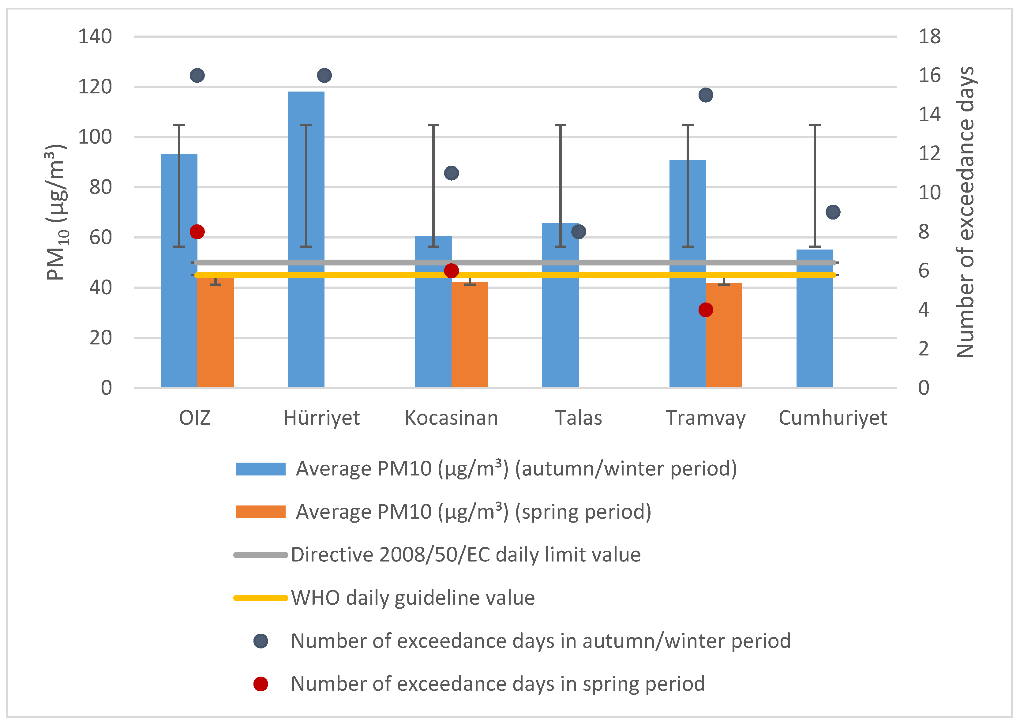
Figure 1. (a) Turkey map and location of Kayseri Province; (b) districts of Kayseri [26].
Atmosphere 14 00356 g001
Figure 2. Wind rose prepared according to the 2014 data of Meteorology Station no. 17195, in Kayseri Province; locations of the six sampling points [28].
Atmosphere 14 00356 g002
Figure 3. Comparison of daily average PM10 concentrations with the EU Directive daily limit value, the WHO daily guideline value for PM10, and the number of exceedance days.
Atmosphere 14 00356 g003
Figure 4. PM10 daily concentrations at Kayseri sampling points and inversion intensity (autumn/winter period).
Atmosphere 14 00356 g004
Figure 5. PM10 daily concentrations at Kayseri sampling points and inversion intensity (spring period).
Atmosphere 14 00356 g005
Figure 6. The AERMOD dispersion map created for scenario 1 (Red crosses represent the facilities considered in the model).
Atmosphere 14 00356 g006
Figure 7. The AERMOD dispersion map created for scenario 2 (Red crosses represent the facilities considered in the model).
Atmosphere 14 00356 g007
Table 1. Coordinates of the sampling points, pollution source types, and the sampling schedule.
Sampling PointsCoordinatesMain Pollution Source TypeSampling Schedule
OIZ X: 38.740437
Y: 35.375453
Industry07.10.2020 to 22.10.2020
28.05.2021 to 11.06.2021
Hürriyet X: 38.714757
Y: 35.470575
Heating07.10.2020 to 22.10.2020
19.11.2020 to 04.12.2020
TalasX: 38.698954
Y: 35.553436
Heating11.11.2020 to 26.11.2020
04.02.2021 to 19.02.2021
KocasinanX: 38.744597
Y: 35.481918
Heating11.11.2020 to 26.11.2020
04.02.2021 to 19.02.2021
28.05.2021 to 11.06.2021
TramvayX: 38.720589
Y: 35.481611
Traffic25.02.2021 to 12.03.2021
28.05.2021 to 11.06.2021
CumhuriyetX: 38.721486
Y: 35.486120
Traffic25.02.2021 to 12.03.2021
Table 2. Correlation coefficients between PM10 and inversion intensity.
Sampling PointsCorrelation Coefficient (r)
Autumn/WinterSpring
OIZ0.72Strong0.03Very weak
Hürriyet0.33Weak
Talas0.24Very weak
Kocasinan−0.02Very weak0.10Very weak
Tramvay0.49Weak0.01Very weak
Cumhuriyet0.06Very weak
Table 3. Daily average metal and metalloid concentrations for autumn/winter and spring periods.
Metals and MetalloidsAutumn/Winter Period Daily Avg. Metal ConcentrationsSpring Period Daily Avg. Metal
Concentrations
AverageStandard Deviation
(ng/m3)(ng/m3)
OIZHürriyetKocasinanTalasTramvayCumhuriyetOIZKocasinanTramvay
Aluminum (Al)11191020456557773657908741712771213
Antimony (Sb)4.09.07.06.08.05.03.02.04.05.02.3
Arsenic (As)2.03.07.04.05.04.02.01.01.03.02.0
Barium (Ba)7183283952334821434720
Boron (B)191417241411137.07.0145.5
Cadmium (Cd)1.01.02.01.01.01.01.0below DL1.01.00.5
Calcium (Ca)1678390216311502below DLbelow DLbelow DLbelow DLbelow DL9681347
Chromium (Cr)22108.09.09.010128.010114.3
Cobalt (Co)194.01.01.01.01.03.01.02.04.05.9
Copper (Cu)212417233327271235257.3
Iron (Fe)1134139563410991634961101370913871107326
Lead (Pb)5533352631263721223210.4
Magnesium (Mg)43743622629743330845747944739189.5
Mangan (Mn)402816212921382026278.2
Molybdenum (Mo)1.02.01.02.02.01.01.0below DL1.01.00.7
Nickel (Ni)126.06.07.0107.09.05.05.07.02.4
Potassium (K)37443245235543537934122427536375.7
Selenium (Se)below DLbelow DL1.0below DLbelow DLbelow DLbelow DLbelow DLbelow DLbelow DL0.3
Sodium (Na)158275371169below DLbelow DL475493365368352.2
Vanadium (V)3.03.03.05.06.03.02.02.02.03.01.4
Zinc (Zn)23586808399912609113212969.4
Table 4. AERMOD modeled PM10 levels, peak receptor coordinates, and dates/hour for scenarios 1 and 2.
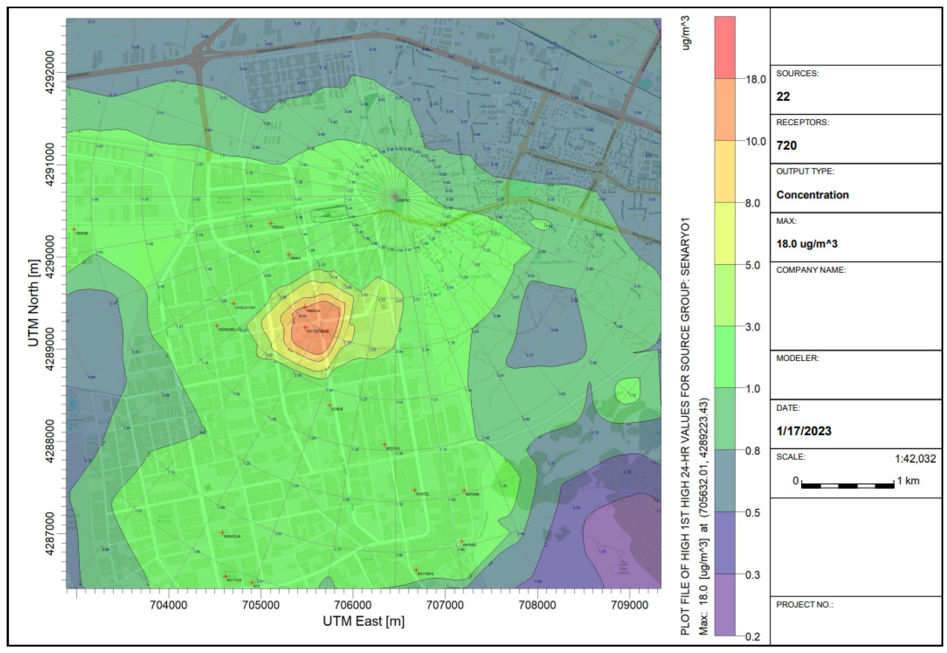
PM10—Concentration—Source Group: Scenario 1
Averaging
Period
RankPM10 (μg/m3)X
(m)
Y
(m)
ZELEV
(m)
ZFLAG
(m)
ZHILL
(m)
Date,
Start Hour
1 h1st52.00485705,632.014,289,223.431047.700.001621.0014 May 2014, 23
24 h1st17.99654705,632.014,289,223.431047.700.001621.0028 November 2014, 24
1 h10th49.75697705,632.014,289,223.431047.700.001621.009 September 2014, 1
24 h10th11.91304705,632.014,289,223.431047.700.001621.0012 November 2014, 24
1 h35th45.14457705,632.014,289,223.431047.700.001621.0013 February2014, 18
24 h35th9.46881705,632.014,289,223.431047.700.001621.0011 September 2014, 24
1 h50th43.88258705,632.014,289,223.431047.700.001621.0016 October 2014, 1
24 h50th8.87223705,632.014,289,223.431047.700.001621.003 October 2014, 24
Annual 5.64820705,632.014,289,223.431047.700.001621.00
PM10—Concentration—Source Group: Scenario 2
Averaging
Period
RankPM10 (μg/m3)X
(m)
Y
(m)
ZELEV
(m)
ZFLAG
(m)
ZHILL
(m)
Date,
Start Hour
1 h1st3.01835696,637.224,287,078.261042.300.001042.3012 November 2014, 11
24 h1st1.03820696,120.394,286,890.151053.500.001060.004 January 2014, 24
1 h10th2.50546696,637.224,287,078.261042.300.001042.305 December 2014, 10
24 h10th0.36564697,154.054,287,266.371034.400.001034.4012 November 2014, 24
1 h35th1.73207696,120.394,286,890.151053.500.001060.004 January 2014, 16
24 h35th0.19729696,120.394,286,890.151053.500.001060.0013 November 2014, 24
1 h50th1.57954696,120.394,286,890.151053.500.001060.003 January 2014, 4
24 h50th0.14811697,154.054,287,266.371034.400.001034.4024 January 2014, 24
Annual 0.05184696,120.394,286,890.151053.500.001060.00
Disclaimer/Publisher’s Note: The statements, opinions and data contained in all publications are solely those of the individual author(s) and contributor(s) and not of MDPI and/or the editor(s). MDPI and/or the editor(s) disclaim responsibility for any injury to people or property resulting from any ideas, methods, instructions or products referred to in the content.

