Exact Expressions for Lightning Electromagnetic Fields: Application to the Rusck Field-to-Transmission Line Coupling Model

Abstract

An exact analytical expression for the electric field of the return stroke as excited by a propagating step current source is derived in this paper. This expression could be advantageously used to evaluate the disturbances caused by lightning on overhead lines. There are three equivalent procedures to evaluate the voltages induced by lightning on power lines, namely, the Agrawal–Price–Gurbaxani model, the Taylor–Satterwhite–Harrison model, and the Rachidi model. In the case of a vertical return stroke channel, the coupling model developed by Rusck becomes identical to these three coupling models. Due to its simplicity, the Rusck model is frequently used by engineers to study the effects of lightning on power distribution and transmission lines. In order to reduce the time involved in the electromagnetic field calculation, the Rusck model is incorporated with an analytical expression for the electromagnetic fields of the return stroke excited by a propagating step current pulse. Our research work shows that the Rusck expression can be used to calculate the peak values of lightning induced voltages to an accuracy of about 10%. However, the use of this analytical expression to calculate the time derivatives of lightning induced voltages may result in errors as large as 50%. The derived expression in this paper can be used to correct for this inaccuracy. We also provide an exact expression for the electric field at any given point in space when the propagating current is an impulse function. This expression can be combined with the convolution integral to obtain the electric field corresponding to waveforms similar to measured return stroke currents.

1. Introduction

Lightning is one of the natural causes of disturbance and disruption in power transmission and distribution lines [1,2,3]. Lightning can affect these systems either through direct strikes or indirectly through electromagnetic field coupling [4]. The mitigation of these indirect effects requires information concerning the temporal behavior of the lightning induced voltages in power transmission and distribution lines. Since the direct measurements of these voltages and currents in live power systems are difficult, engineers have developed procedures to evaluate the features of these disturbances through computer simulations. Such analyses require information on the electromagnetic fields generated by lightning return strokes and coupling models to represent the interaction of these electromagnetic fields with the lines. There are several field-to-line coupling models in the literature, namely those introduced by Rusck [5], Agrawal et al. [6], Taylor et al. [7], and Rachidi [8]. The latter three models have been shown to be equivalent to each other, even though each represents the field-to-line coupling equations in terms of different excitation sources [9]. The Rusck model, which neglects one of the source terms, is equivalent to the other three only in the case where the lightning channel is vertical [10]. However, since the analysis of indirect effects of lightning on power distribution and transmission lines is commonly conducted by assuming that the lightning channel is vertical, Rusck’s coupling model can be used in these engineering studies without any disadvantages in comparison to the other coupling models. This fact, combined with its simplicity, made this model an important engineering tool in the assessment of lightning induced voltages in power transmission and distribution lines [1,2,3,11,12,13]. As mentioned earlier, in order to evaluate lightning induced voltages on power transmission lines, in addition to the field-to-line coupling model, one needs to know the electromagnetic fields generated by lightning at different distances from the lightning channel (along the line). In general, these fields are calculated using return stroke models. There are many return stroke model types in the literature. These models can be classified into gas dynamic models (or physics based models), Electromagnetic models, waveguide models, transmission line models, and engineering models [14,15,16,17]. Due to their simplicity and their ability to successfully reproduce the salient features of the lightning electromagnetic pulse (LEMP), return stroke models belonging to the engineering model type are frequently used in practical studies. The engineering models can be divided into current propagation, current generation, and current dissipation types [14]. It is the current propagation type models that are being used frequently in the analysis of lightning-induced voltages in power systems. The most frequently used current propagation type models are the transmission line model (TL model) [18] and its modifications, namely, the modified transmission line model with exponential current decay (MTLE model) [19,20] and the modified transmission line model with linear current decay (MTLL model) [21]. Cooray and Orville [22] developed a modified transmission line model where both the current attenuation and dispersion are taken into account. More recently, a new modified transmission line model (called the MTLD model) in which the current attenuation function is derived from the lightning electromagnetic field was developed by Cooray et al. [23].

In the analysis of induced over-voltages in power lines due to lightning, the electromagnetic fields generated by lightning appear as inputs to the coupling model. Since this requires the calculation of electromagnetic fields from lightning at a large number of distances, the use of analytical expressions for the electromagnetic fields generated by return stroke models makes the calculation process much faster [24,25,26]. In Rusck’s field-to-line coupling model, the electromagnetic fields are calculated using the classical TL model. In its original formulation, the return stroke current in the Rusck model is assumed to be a step function and analytical field expressions are derived for the vertical field over a perfectly conducting ground. This field expression can be extended to any other return stroke current waveform by using the Duhammel’s integral [12].

It is also important to mention that Rusck’s coupling model is based on the assumption of a perfectly conducting ground. The electromagnetic field generated by lightning at a given distance will be modified both by the conductivity of the ground [27] and the terrain features [28,29]. The most important effect of the finitely conducting ground is the generation of a horizontal electric field that has a considerable influence on the magnitude and features of the induced voltages [1]. Even though the Rusck model was originally developed to work with lines over a perfectly conducting ground, it can easily be modified to account for the finitely conducting ground by adding the contributions from the horizontal electric field into the induced voltages [30].

The analytical expression given by Rusck provides a quick means to compute the electric field from the lightning return stroke. However, as mentioned earlier, the field expression of Rusck is not exact and, as we will show later, it can lead to significant errors (as large as 50%) in the field derivatives. The goal of the present paper is to provide accurate field expressions for the TL model excited by a step current pulse and thus remove this drawback in the Rusck’s coupling model.

In the paper, we will also provide an exact expression for the electric field at any given point in space when the propagating current is an impulse function. This expression can be combined with the convolution integral to get the electric fields corresponding to current waveshapes similar to those measured in lightning return strokes. The field equations will be obtained over a perfectly conducting ground. The reason for this choice is the following: First, the original Rusck formulation was given assuming a perfectly conducting ground. Second, to account for the presence of a finitely conducting ground, the common approach is to use the Cooray–Rubinstein formula [31,32], which actually uses as inputs the field components (magnetic field and horizontal electric field) evaluated for a perfectly conducting ground.

It is important to point out that the goal of this paper is to present exact electromagnetic field expressions for a transmission line return stroke model where the current is described by a step function. This is identical to the return stroke model used by Rusck in his lightning field-to-transmission line coupling model. Note that we will give the equations necessary in the derivation of the final expressions since this will enable other researchers to reproduce and implement the procedure in their research work.

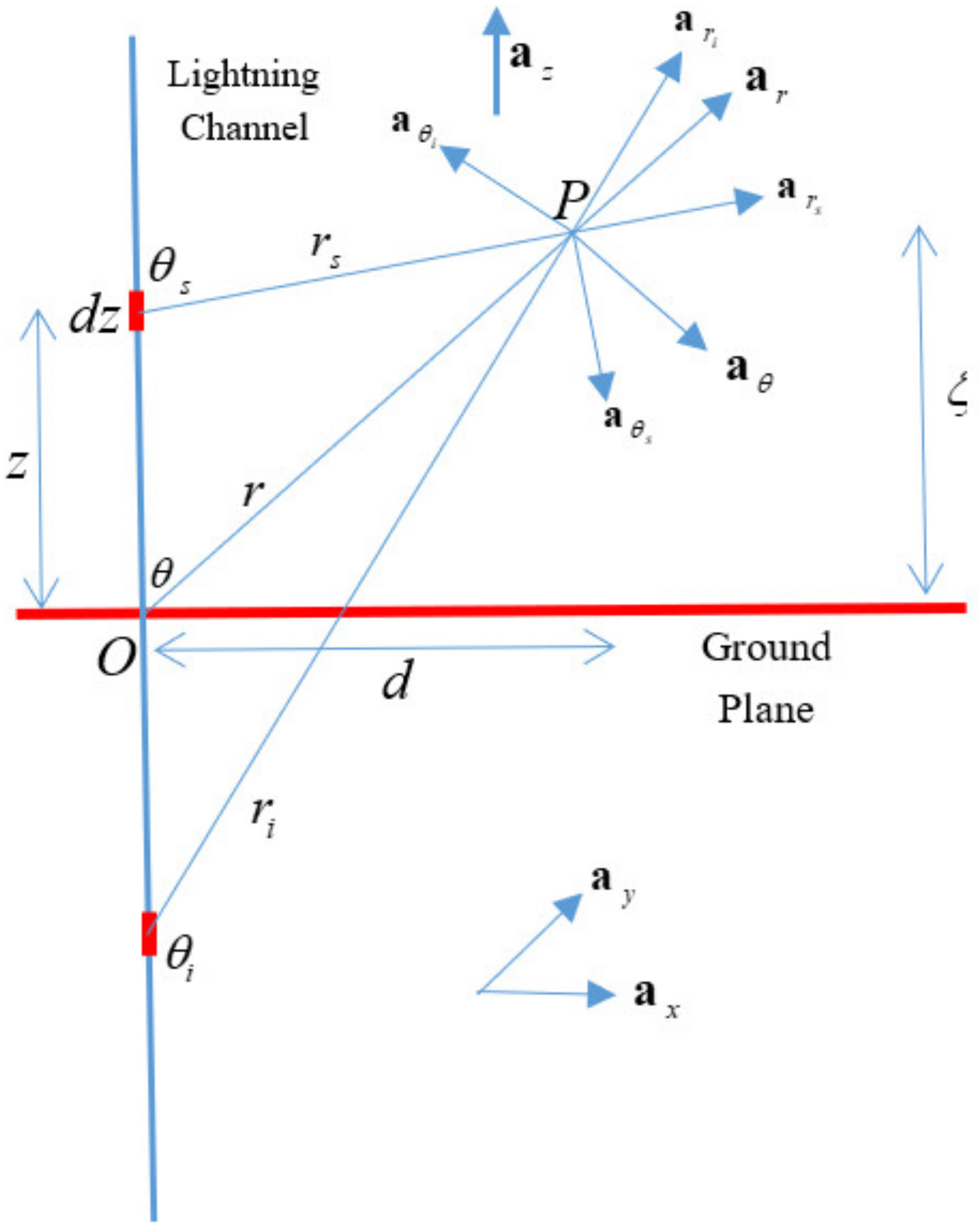
2. Problem Formulation

Let us consider the transmission line (TL) model of the return stroke. In this model, the return stroke is simulated by a current pulse that propagates upwards with uniform speed and without dispersion or attenuation. In the calculation of voltages induced by lightning on power lines, the induced voltages within the first few tens of microseconds are of interest. Due to this, there is no need to consider the effects of the channel termination inside the cloud. For this reason, without loss of generality, we can assume that the return stroke channel extends to infinity. According to this model, the return stroke current at any given height z along the return stroke channel is given by

$$\begin{array}{c}i(z,t)=0\mathrm{for}t\le z/v\hfill \\ i(z,t)=i_b(t-z/v)\mathrm{for}t>z/v\hfill \end{array}$$

(1)

In the above equation, $i_b(t)$ is the current at the channel base, $v$ is the return stroke speed, and $z$ is the height along the return stroke channel. In the present analysis, we consider the channel–base current to be a step function with an amplitude $i_0$. With such channel–base current, Equation (1) reduces to

$$\begin{array}{c}i(z,t)=0\mathrm{for}t\le z/v\hfill \\ i(z,t)=i_0\mathrm{for}t>z/v\hfill \end{array}$$

(2)

The next step is to derive an expression for the electromagnetic fields generated by this current distribution.

3. Electric Field of the Return Stroke

The geometry relevant to the problem at hand is shown in Figure 1. The vertical lightning channel is located over a perfectly conducting ground plane. The z-axis is directed perpendicularly out of the ground plane and the unit vector directed along the positive z-axis is $a_z$. The lightning strike point coincides with the origin O of the coordinate system. The point of observation $P$ is located on the x-z plane, at a height $\zeta$ from the ground and at a horizontal distance d from the lightning strike point. Due to rotational symmetry, the fact that we have selected the observation point to be in the x-z plane does not affect the generality of the results to be derived. The distance $OP$ from the strike point O to the observation point is $r$. A generic infinitesimal channel element located at a height z is denoted by $dz$ and the distance from this channel element to the point of observation is denoted by $r_s$. The effect of the perfectly conducting ground plane is taken into account by the image of the return stroke channel with respect to the ground plane. The distance from the image of the infinitesimal channel element to the point of observation is $r_i$. The vectors $a_r$, $a_{r_s}$, and $a_{r_i}$ are directed along the direction of increasing $r$, $r_s$, and $r_i$ respectively. The vectors $a_{\theta }$, $a_{{\theta }_s}$, and $a_{{\theta }_i}$ can be calculated by way of $a_r\times (a_r\times a_z)$,$a_{r_s}\times (a_{r_s}\times a_z)$, and $a_{r_i}\times (a_{r_i}\times a_z)$, respectively. The distances $r_s$ and $r_i$ are given by

$$r_s=\sqrt{d^2+{(\zeta -z)}^2}$$

(3)

$$r_i=\sqrt{d^2+{(\zeta +z)}^2}$$

(4)

The angles ${\theta }_s$ and ${\theta }_i$ are given by

$${\theta }_s=co{s}^{-1}\left(\left\{\zeta -z\right\}/r_s\right)$$

(5)

$${\theta }_i=co{s}^{-1}\left(-\left\{\zeta +z\right\}/r_i\right)$$

(6)

The goal of this paper is to derive an analytical expression for the vertical electric field at point P. First, we will give the approximate expression derived by Rusck [5] for this field component. After that, we will develop an exact expression for this field component.

3.1. Expressions for the Vertical and Horizontal Electric Fields Based on Rusck’s Formulation

According to Rusck, the vertical electric field as a function of time at point P, following the physics sign convention, is given by [5] (see also [11])

$$\begin{array}{c}{E}_{v,Rusck}(\zeta ,t)=E_0(\zeta ,t_0)\hfill \\ +\frac{Z_E{i}_0\lambda }{4\pi v_r}\left\{{\left[{(vt-\zeta )}^2+\lambda d^2\right]}^{-\frac{1}{2}}+{\left[{(vt+\zeta )}^2+\lambda d^2\right]}^{-\frac{1}{2}}\right\}\hfill \end{array}$$

(7)

with

$$\begin{array}{c}{E}_0(\zeta ,t_0)=-\frac{Z_E{i}_0\lambda }{4\pi v_r}\hfill \\ \left\{{\left[{(v{t}_0-\zeta )}^2+\lambda d^2\right]}^{-\frac{1}{2}}+{\left[{(v{t}_0+\zeta )}^2+\lambda d^2\right]}^{-\frac{1}{2}}\right\}\hfill \end{array}$$

(8)

In the above equations, $t_0=\sqrt{d^2+{\zeta }^2}$, $v_r=v/c$, $\lambda =1-\frac{v^2}{c^2}$, and $Z_E$ is the impedance of free space.

Following the same procedure used by Rusck to obtain the vertical electric field, one can derive an expression for the horizontal electric field [33]. This results in the following expression for the electric field parallel to the ground and directed away from the lightning channel (i.e., along the x-axis when the point of observation P is located on the x–z plane

$$\begin{array}{c}{E}_{h,Rusck}(\zeta ,t)=\hfill \\ \frac{Z_E{i}_0}{2\pi v_r}\left[\frac{\lambda d}{\left\{\left(vt-\zeta +\sqrt{{(\zeta -vt)}^2+\lambda d^2}\right)\left(\sqrt{{(\zeta -vt)}^2+\lambda d^2}\right)\right\}}\right]\hfill \\ +\frac{Z_E{i}_0}{2\pi v_r}\left[\frac{d}{\left\{\left(\sqrt{{\zeta }^2+d^2}\right)\left(\zeta -\sqrt{{\zeta }^2+d^2}\right)\right\}}\right]\hfill \\ -\frac{Z_E{i}_0}{2\pi v_r}\left[\frac{\lambda d}{\left\{\left(vt+\zeta +\sqrt{{(\zeta +vt)}^2+\lambda d^2}\right)\left(\sqrt{{(\zeta +vt)}^2+\lambda d^2}\right)\right\}}\right]\hfill \\ +\frac{Z_E{i}_0}{2\pi v_r}\left[\frac{d}{\left\{\left(\sqrt{{\zeta }^2+d^2}\right)\left(\zeta +\sqrt{{\zeta }^2+d^2}\right)\right\}}\right]\hfill \end{array}$$

(9)

This expression was derived by Barbosa and Paulino [33] by taking the gradient of the scalar potential at point P.

3.2. Exact Expressions for the Electric Field at Any Point in Space

At present, there are four methods developed in the literature to evaluate the electromagnetic fields once the spatial and temporal distribution of the current are given [34,35,36]. These are known as the dipole (Lorentz) technique, the continuity equation technique and two versions of the procedures based on moving and accelerating charges. Although the various components that constitute the total field are different in each technique, all these techniques give rise to the same total field. Here, we will use the moving and accelerating charge procedure, which will make it possible to express the resulting electromagnetic fields analytically. In the case of the transmission line model [18] excited by a step current pulse, the total electric field consists of radiation field and velocity field components. The radiation field is generated by the accelerating charges and the velocity field is generated by the uniformly moving charges. In the problem under consideration, there are no fields generated by static charges because there is no accumulation of charges along the return stroke channel. Since the current moves with constant speed along the channel and since radiation only comes from accelerating charges, the radiation from the channel is generated only at the initiation of the lightning current at the bottom of the channel. The radiation field generated at point P by the initiation of the source current is given by [36]

$$E_{s,r,\theta }(t,\zeta )=\frac{i(t-r/c)v\sin \theta }{4\pi {\epsilon }_0{c}^{2}r(1-v_r\cos \theta )}{a}_{\theta }$$

(10)

The component of this field directed along the z-axis (the vertical field) is given by

$$E_{s,r,z}(t,\zeta )=-\frac{i(t-r/c)v{\sin }^2\theta }{4\pi {\epsilon }_0{c}^{2}r(1-v_r\cos \theta )}$$

(11)

Note that in Equation (11) and in the subsequent equations, the first of the comma-separated sub-indexes indicates whether the field is from the source or from the image (in this case, ‘s’ stands for source and ‘i’ stands for image). The second sub-index indicates if the field is the radiation ($‘r’$) or the velocity field ($‘v’$). The third sub-index, when present, denotes the specific component of the field.

The velocity field generated by the current element $dz$ located at a height z along the channel is given by

$$d{E}_{s,v}^{}(t,\zeta )=-\frac{i(0,t-z/v-r_s/c)\lambda }{4\pi {\epsilon }_o{r}_s^{2}c{\left[1-v_r\cos {\theta }_s\right]}^2}{a}_z+\frac{i(0,t-z/v-r_s/c)\lambda }{4\pi {\epsilon }_o{r}_s^{2}v{\left[1-v_r\cos {\theta }_s\right]}^2}{a}_{r_s}$$

(12)

The total velocity field generated by the source at point P directed along the z-axis is then given by

$$E_{s,v,z}^{}(t,\zeta )=-{\displaystyle \underset{0}{\overset{z_{su}(t)}{\int }}\frac{dzi(0,t-z/v-r_s/c)\lambda }{4\pi {\epsilon }_o{r}_s^2{\left[1-v_r\cos {\theta }_s\right]}^2}\left[\frac{1}{c}-\frac{\cos {\theta }_s}{v}\right]}$$

(13)

In the above equation, the upper integration limit $z_{su}(t)$ (the subscripts s and u stand for source and upper limit, respectively) is the length of the source channel that contributes to the electric field at point P at time t. This length can be obtained by solving the equation

$$z_{su}(t)/v+r_{su}(t)/c-r/c=t$$

(14)

with

$$r_{su}(t)=\sqrt{{(\zeta -z_{su}(t))}^2+d^2}$$

(15)

Plugging Equation (15) into Equation (14) leads to the following quadratic equation,

$$\begin{array}{c}{z}_{su}^2(t)\left\{1/v^2-1/c^2\right\}+z_{su}(t)\left\{2\zeta /c^2-2(t+r/c)/v\right\}\hfill \\ +\left\{{(t+r/c)}^2-{\zeta }^2/c^2-d^2/c^2\right\}=0\hfill \end{array}$$

(16)

which can be solved to obtain $z_{su}$.

Now, in our case, the current is a step function and Equations (11) and (13) can be written as

$$E_{s,r,z}(t,\zeta )=-\frac{i_{0}v{\sin }^2\theta }{4\pi {\epsilon }_0{c}^{2}r(1-v_r\cos \theta )}$$

(17)

$$E_{s,v,z}^{}(t,\zeta )=-{\displaystyle \underset{0}{\overset{z_{su}(t)}{\int }}\frac{dz{i}_0\lambda }{4\pi {\epsilon }_o{r}_s^2{\left[1-v_r\cos {\theta }_s\right]}^2}\left[\frac{1}{c}-\frac{\cos {\theta }_s}{v}\right]}$$

(18)

Similarly, the image channel also contributes to the field and the two corresponding field components are

$$E_{i,r,z}(t,\zeta )=-\frac{i_{0}v{\sin }^2\theta }{4\pi {\epsilon }_0{c}^{2}r(1+v_r\cos \theta )}$$

(19)

$$E_{i,v,z}^{}(t,\zeta )=-{\displaystyle \underset{0}{\overset{z_{iu}(t)}{\int }}\frac{dz{i}_0\lambda }{4\pi {\epsilon }_o{r}_1{\left[1-v_r\cos {\theta }_i\right]}^2}\left[\frac{1}{c}-\frac{\cos {\theta }_i}{v}\right]}$$

(20)

In the above equation, $z_{iu}(t)$ (the subscripts i and u stand for image and upper limit, respectively) is the length of the image channel that contributes to the electric field at point P at time t. This length can be obtained by solving the equation

$$z_{iu}(t)/v+r_{iu}(t)/c-r/c=t$$

(21)

with

$$r_{iu}(t)=\sqrt{{(\zeta +z_{iu}(t))}^2+d^2}$$

(22)

Substitution of Equation (22) into Equation (21) results in the following quadratic equation that can be solved to obtain $z_{iu}(t)$,

$$z_{iu}^2(t)\left\{1/v^2-1/c^2\right\}+z_{iu}(t)\left\{-2\zeta /c^2-2(t+r/c)/v\right\}+\left\{{(t+r/c)}^2-{\zeta }^2/c^2-d^2/c^2\right\}=0$$

(23)

Adding the contributions of the source and the image given by Equations (17) and (19), the vertical component of the total radiation field is then given by

$$E_{r,z}(t,\zeta )=-\frac{i_{0}v{\sin }^2\theta }{2\pi {\epsilon }_0{c}^{2}r(1-v_r^2{\cos }^2\theta )}$$

(24)

Similarly, the vertical component of the total velocity field is given by

$$\begin{array}{c}{E}_{v,z}^{}(t,\zeta )=-\frac{i_0\lambda }{4\pi {\epsilon }_o}{\displaystyle \underset{0}{\overset{z_{su}(t)}{\int }}\frac{dz}{r_s^2{\left[1-v_r\cos {\theta }_s\right]}^2}\left[\frac{1}{c}-\frac{\cos {\theta }_s}{v}\right]}\hfill \\ -\frac{i_0\lambda }{4\pi {\epsilon }_o}{\displaystyle \underset{0}{\overset{z_{iu}(t)}{\int }}\frac{dz}{r_i^2{\left[1-v_r\cos {\theta }_i\right]}^2}\left[\frac{1}{c}-\frac{\cos {\theta }_i}{v}\right]}\hfill \end{array}$$

(25)

Equations (24) and (25) define the vertical electric field generated by the return stroke at any given point in space.

The horizontal electric field (directed away from the channel) at point P generated by the source can be obtained directly from Equation (10) and the result is

$$E_{s,r,h}(t,\zeta )=\frac{i(t-r/c)v\sin \theta \cos \theta }{4\pi {\epsilon }_0{c}^{2}r(1-v_r\cos \theta )}$$

(26)

The horizontal component of the velocity field generated by the current element $dz$ located at a height z along the channel can be obtained from Equation (12) and it is given by

$$d{E}_{s,v,h}^{}(t,\zeta )=\frac{i(0,t-z/v-r_s/c)\lambda \sin \theta }{4\pi {\epsilon }_o{r}_s^{2}v{\left[1-v_r\cos {\theta }_s\right]}^2}dz$$

(27)

The horizontal component of the total velocity field generated by the source at point P is then given by

$$E_{s,v,h}^{}(t,\zeta )={\displaystyle \underset{0}{\overset{Z_{su}(t)}{\int }}\frac{dzi(0,t-z/v-r_s/c)\lambda \sin \theta }{4\pi {\epsilon }_o{r}_s^{2}v{\left[1-v_r\cos {\theta }_s\right]}^2}}$$

(28)

Similarly, the image channel also contributes to the horizontal field and the two corresponding field components are

$$E_{i,r,h}(t,\zeta )=\frac{i_{0}v\sin \theta \cos \theta }{4\pi {\epsilon }_0{c}^{2}r(1+v_r\cos \theta )}$$

(29)

and

$$E_{i,v,h}^{}(t,\zeta )=-{\displaystyle \underset{0}{\overset{Z_{iu}(t)}{\int }}\frac{dz{i}_0\lambda \sin {\theta }_i}{4\pi {\epsilon }_o{r}_{i}v{\left[1-v_r\cos {\theta }_i\right]}^2}}$$

(30)

The horizontal component of the total radiation field is then given by

$$E_{r,h}(t,\zeta )=\frac{i_{0}v\sin \theta \cos \theta }{2\pi {\epsilon }_0{c}^{2}r(1-v_r^2{\cos }^2\theta )}$$

(31)

and the horizontal component of the total velocity field is given by

$$E_{v,h}^{}(t,\zeta )=\frac{i_0\lambda }{4\pi {\epsilon }_{o}v}{\displaystyle \underset{0}{\overset{Z_{su}(t)}{\int }}\frac{dz\sin {\theta }_s}{r_s^2{\left[1-v_r\cos {\theta }_s\right]}^2}}-\frac{i_0\lambda }{4\pi {\epsilon }_{o}v}{\displaystyle \underset{0}{\overset{Z_{iu}(t)}{\int }}\frac{dz\sin {\theta }_i}{r_i^2{\left[1-v_r\cos {\theta }_i\right]}^2}}$$

(32)

These expressions for the vertical and horizontal electric fields are exact and they can be used to test the validity of Rusck’s expressions numerically. This is done in the next section.

4. Comparison of Rusck’s Expression with the Exact Vertical Electric Field at any Given Point in Space

In the analysis of the coupling of lightning electromagnetic fields (LEMP) to transmission and distribution lines, it is the first 10 microseconds or so that are of interest in the development of procedures to mitigate the effects of these voltages. This is the case because, in most of the cases, the peak of the lightning induced voltages and the peak derivative are reached within this time. For this reason, we will concentrate here mainly on those initial microseconds of the electric field.

Figure 2 shows the vertical electric field at ground level calculated at different distances for a step current using the two formulations presented earlier, namely (i) Rusck’s original formulas (Equations (7) and (9)), and (ii) the derived expressions using the field components associated with moving and accelerating charges (Equations (24) and (25)). In this calculation, the propagation speed of the current pulse is assumed to be 1.5 × 10⁸ m/s. Figure 3 depicts the vertical electric field obtained from the two formulations when the step function return stroke current is replaced by currents corresponding to those of first and subsequent return strokes. In the case of first return stroke, the speed of propagation was fixed at 1.0 × 10⁸ m/s. The derivatives of the vertical electric field of a subsequent return stroke, obtained from the two formulations are shown in Figure 4 and the results pertinent to the horizontal electric field are shown in Figure 5 (the used expressions are (31) and (32)). According to these results, the error in the vertical electric field when using the Rusck model is less than about 10% and the error in the horizontal electric field is about 15%, indicating that the Rusck formulation can provide acceptable accuracy in calculating the peak voltages induced in power lines by lightning flashes. On the other hand, note that the error in the electric field time derivative calculated using the Rusck formulation is about 50%. These error levels in the field derivatives are reflected in the derivatives of the correcponding induced voltages calculated using the Rusck model. A higher accuracy can be achieved using the electromagnetic field equations presented in this paper.

In some studies, the electric fields corresponding to more realistic return stroke current waveforms are obtained by using the Duhammel’s theorem. Analytical representations for typical first return and subsequent return stroke currents can be found in [37]. Using these current waveforms together with the Duhammel’s integral, we obtained the electric field at different distances corresponding to first and subsequent return strokes. Two examples of the results obtained are shown in Figure 5. Again, observe that the errors resulting in the peak value of the electric field when using the Rusck formulation are less than about 10%.

One advantage of the Rusck’s electric field expression is that it is anlytical and it does not involve the numerical solution of integrals similar to those in Equations (18) and (20). Fortunately, the integrals in these equations can be solved analytically for the case of a step current and this makes it possible to create an exact analytical expression for the electric field of that current waveform. This is done in the next section.

5. Exact Analytical Expression for the Electric Field of a Step Current Pulse at any Point in Space

First, observe that it is only the velocity field which is given as an integral whereas the radiation field can easily be obtained from the analytical expresion given by Equations (24) and (31). In order to solve the integrals in the velocity field, let us rewrite them with angles ${\theta }_s$ and ${\theta }_i$ as variables of integration. This can be done easily using the relationships $\tan {\theta }_s=d/(\zeta -z)$ and $\tan {\theta }_i=-d/(\zeta +z)$. The resulting integrals are

$$\begin{array}{c}{E}_{v,z}^{}=-\frac{i_0\lambda H(t-r/c)}{4\pi {\epsilon }_o}{\displaystyle \underset{{\theta }_{sl}}{\overset{{\theta }_{su}(t)}{\int }}\frac{d{\theta }_s}{d{\left[1-v_r\cos {\theta }_s\right]}^2}\left[\frac{1}{c}-\frac{\cos {\theta }_s}{v}\right]}\hfill \\ -\frac{i_0\lambda H(t-r/c)}{4\pi {\epsilon }_o}{\displaystyle \underset{{\theta }_{il}}{\overset{{\theta }_{iu}(t)}{\int }}\frac{d{\theta }_i}{d{\left[1-v_r\cos {\theta }_i\right]}^2}\left[\frac{1}{c}-\frac{\cos {\theta }_i}{v}\right]}\hfill \end{array}$$

(33)

In the above equation, $H(t)$ represents the unit step function. Its properties are: $H(t)=0$ for $t<0$ and $H(t)=1$ for $t\ge 0$. Note that the angles ${\theta }_{su}(t)$ and ${\theta }_{iu}(t)$ are time-dependent variables because their values change as the return stroke channel grows upwards (i.e., as $z_{su}(t)$ and $z_{iu}(t)$ increase). These integrals can be evaluated analytically and the total velocity electric field at times $t\ge r/c$ can be written as (with $k=i_{0}H(t-r/c)/4\pi {\epsilon }_{0}d$)

$$\begin{array}{c}{E}_{v,z}(t,\zeta )=\hfill \\ k\left[\frac{1}{c}\frac{2}{\sqrt{\lambda }}{\tan }^{-1}\left\{\tan \left(\frac{{\theta }_{su}(t)}{2}\right)\sqrt{\frac{1+v_r}{1-v_r}}\right\}+\frac{1}{v}\frac{\lambda \sin {\theta }_{su}(t)}{1-v_r\cos {\theta }_{su}(t)}\right]\hfill \\ -k\left[\frac{1}{c}\frac{2}{\sqrt{\lambda }}{\tan }^{-1}\left\{\tan \left(\frac{{\theta }_{sl}}{2}\right)\sqrt{\frac{1+v_r}{1-v_r}}\right\}+\frac{1}{v}\frac{\lambda \sin {\theta }_{sl}}{1-v_r\cos {\theta }_{sl}}\right]\hfill \\ k\left[\frac{1}{c}\frac{2}{\sqrt{\lambda }}{\tan }^{-1}\left\{\tan \left(\frac{{\theta }_{iu}(t)}{2}\right)\sqrt{\frac{1+v_r}{1-v_r}}\right\}+\frac{1}{v}\frac{\lambda \sin {\theta }_{iu}(t)}{1-v_r\cos {\theta }_{iu}(t)}\right]\hfill \\ -k\left[\frac{1}{c}\frac{2}{\sqrt{\lambda }}{\tan }^{-1}\left\{\tan \left(\frac{{\theta }_{il}}{2}\right)\sqrt{\frac{1+v_r}{1-v_r}}\right\}+\frac{1}{v}\frac{\lambda \sin {\theta }_{il}}{1-v_r\cos {\theta }_{il}}\right]\hfill \end{array}$$

(34)

Observe that in the above equations, ${\theta }_{sl}$=$\theta$ (the subscript l stands for the lower limit) and ${\theta }_{il}=(\pi -\theta )$. The angles ${\theta }_{su}(t)$ and ${\theta }_{iu}(t)$ are given by

$${\theta }_{su}(t)=co{s}^{-1}\left(\left\{\zeta -Z_{su}(t)\right\}/r_{su}(t)\right)$$

(35)

$${\theta }_{iu}(t)=co{s}^{-1}\left(-\left\{\zeta +Z_{iu}(t)\right\}/r_{iu}(t)\right)$$

(36)

The lengths $z_{su}(t)$ and $z_{iu}(t)$ are given by

$$z_{su}(t)=\frac{-B_s\pm \sqrt{B_s^2-4A_0{C}_0}}{2A_0}$$

(37)

$$z_{iu}(t)=\frac{-B_i\pm \sqrt{B_i^2-4A_0{C}_0}}{2A_0}$$

(38)

where

$$A_0=(1/v^2-1/c^2)$$

(39)

$$B_s=2\zeta /c^2-2(t+r/c)/v$$

(40)

$$B_i=-2\zeta /c^2-2(t+r/c)/v$$

(41)

$$C_0={(t+R/c)}^2-{\zeta }^2/c^2-d^2/c^2$$

(42)

With these parameters ($r_{su}(t)$ and $r_{iu}(t)$ are defined in Equations (14) and (21)), the total vertical electric field at any point in space can be obtained by adding the contribution of the radiation field to the expression given by Equation (34). With this, the total vertical electric field is given by

$$E_z(t,\zeta )=E_{v,z}(t,\zeta )-\frac{i_{0}H(t-r/c)v{\sin }^2\theta }{2\pi {\epsilon }_0{c}^{2}r(1-v_r^2{\cos }^2\theta )}$$

(43)

Equation (43) expresses the vertical electric field at any point in space. It is important to point out that the above analytical expression is valid for any point in space for $v<c$.

In a similar manner, we can derive an analytical expression for the horizontal electric field. Again, note that it is only the velocity field which is given as an integral whereas the radiation field can easily be obtained from the analytical expresion given by Equation (10). In order to solve the integrals in the horizontal velcocity field, let us again rewite them with angles ${\theta }_s$ and ${\theta }_i$ as variables of integration. This can be done easily using the relationships $\tan {\theta }_s=d/(\zeta -z)$ and $\tan {\theta }_i=-d/(\zeta +z)$. The resulting integrals are

$$E_{v,h}^{}=\frac{i_0\lambda H(t-r/c)}{4\pi {\epsilon }_{o}v}{\displaystyle \underset{{\theta }_{sl}}{\overset{{\theta }_{su}(t)}{\int }}\frac{d{\theta }_s\sin {\theta }_s}{d{\left[1-v_r\cos {\theta }_s\right]}^2}}-\frac{i_0\lambda H(t-r/c)}{4\pi {\epsilon }_{o}v}{\displaystyle \underset{{\theta }_{il}}{\overset{{\theta }_{iu}(t)}{\int }}\frac{\sin {\theta }_{i}d{\theta }_i}{d{\left[1-v_r\cos {\theta }_i\right]}^2}}$$

(44)

These integrals can be solved analytically and the resulting expression for the velocity horizontal electric field is

$$\begin{array}{c}{E}_{v,h}(t,\zeta )=\frac{k}{v{v}_r}\left[\frac{1}{1-v_r\cos {\theta }_{sl}}-\frac{1}{1-v_r\cos {\theta }_{su}}\right]\hfill \\ -\frac{k}{v{v}_r}\left[\frac{1}{1-v_r\cos {\theta }_{il}}-\frac{1}{1-v_r\cos {\theta }_{iu}}\right]\hfill \end{array}$$

(45)

The total horizontal electric field at any point in space can be calculated by adding the contribution of the radiation field to the above equation. That is

$$E_h(t,\zeta )=E_{v,h}(t,\zeta )+\frac{i_{0}H(t-r/c)v\sin \theta \cos \theta }{2\pi {\epsilon }_0{c}^{2}r(1-v_r^2{\cos }^2\theta )}$$

(46)

Equation (46) provides an exact analytical exporession for the horizontal electric field at any point in space.

Electric Field at Ground Level

When the point of observation is at ground level (i.e., $r=d$), $\theta =\pi /2$ and ${\theta }_{sl}={\theta }_{il}=\pi /2$. Moreover, $z_{su}(t)=z_{iu}(t)$ and ${\theta }_{su}(t)={\theta }_{iu}(t)$. Denoting the latter two distances and angles by $z_u(t)$ and ${\theta }_u(t)$, the velocity electric field at ground level can be expressed as

$$\begin{array}{c}{E}_{v,z}(t,0)=2k\left[\frac{1}{v}\frac{\lambda \sin {\theta }_u(t)}{1-v_r\cos {\theta }_u(t)}+\frac{1}{c}\frac{2}{\sqrt{\lambda }}{\tan }^{-1}\left\{\tan \left(\frac{{\theta }_u(t)}{2}\right)\sqrt{\frac{1+v_r}{1-v_r}}\right\}\right]\hfill \\ -2k\left[\frac{\lambda }{v}+\frac{1}{c}\frac{2}{\sqrt{\lambda }}{\tan }^{-1}\left\{\sqrt{\frac{1+v_r}{1-v_r}}\right\}\right]\hfill \end{array}$$

(47)

In the above equation, the cosine of the angle ${\theta }_u(t)$ is given by

$${\theta }_u(t)={\cos }^{-1}(-z_u(t)/\sqrt{z_u^2(t)+d^2})$$

(48)

with

$$z_u(t)=\frac{-B_0\pm \sqrt{B_0^2-4A_0{C}_0}}{2A_0}$$

(49)

where

$$A_0=(1/v^2-1/c^2)$$

(50)

$$B_0=-2(t+r/c)/v$$

(51)

$$C_0={(t+R/c)}^2-d^2/c^2$$

(52)

With these parameters, Equation (45) gives the exact expression of the vertical velocity electric field at a distance $d$ at ground level. The total vertical electric field is given by

$$E_z(t,0)=E_{v,z}(t,0)-\frac{i_{0}H(t-r/c)v}{2\pi {\epsilon }_0{c}^{2}d}$$

(53)

Obviously, the horizontal electric field goes to zero when the point of observation is at ground level.

6. Exact Analytical Expression for the Electric Field of an Impulse Current Pulse at any Point in Space

In the analysis of induced voltages by lightning using the Rusck’s coupling equations, the electric field of the step current is converted to the electric field pertinent to a typical return stroke current by using Duhammel’s theorem. In such analysis, it is convenient to have the electric field response for a delta impulse current instead of a step current. Knowing the impulse current response, the field due to any other current can be obtained using the convolution integral.

Now, the expressions given by Equations (11) and (13) describe the vertical electric field at any point in space generated by the source current. When the current in the return stroke channel is an impulse, the electric field generated by the source current can be written as

$$E_{s,r,z}(t,\zeta )=-\frac{\delta (t-r/c)v{\sin }^2\theta }{4\pi {\epsilon }_0{c}^{2}r(1-v_r\cos \theta )}$$

(54)

$$E_{s,v,z}^{}(t,\zeta )=-{\displaystyle \underset{0}{\overset{z_{su}(t)}{\int }}\frac{dz\delta (t-z/v-r_s/c)\lambda }{4\pi {\epsilon }_o{r}_s^2{\left[1-v_r\cos {\theta }_s\right]}^2}\left[\frac{1}{c}-\frac{\cos {\theta }_s}{v}\right]}$$

(55)

In the above equations, $\delta (t)$ represents the Dirac impulse function. Observing that $z_{su}(t)$ is the solution of the equation $t-z/v-r_s/c=0$, the integral in the above equation can be solved directly and the result is

$$E_{s,v,z}^{}(t,\zeta )=-\frac{\lambda H(t-r/c)}{4\pi {\epsilon }_o{r}_{su}^2(t){\left[1-v_r\cos {\theta }_{su}(t)\right]}^2}\left[\frac{1}{c}-\frac{\cos {\theta }_{su}(t)}{v}\right]$$

(56)

Similarly, the velocity field produced by the image channel is given by

$$E_{i,v,z}^{}(t,\zeta )=-\frac{\lambda H(t-r/c)}{4\pi {\epsilon }_o{r}_{iu}^2(t){\left[1-v_r\cos {\theta }_{iu}(t)\right]}^2}\left[\frac{1}{c}-\frac{\cos {\theta }_{iu}(t)}{v}\right]$$

(57)

Thus, the total electric field at the point of observation at times $t\ge r/c$ is given by

$$\begin{array}{c}{E}_z(t,\zeta )=-\frac{\delta (t-r/v)v{\sin }^2\theta }{2\pi {\epsilon }_0{c}^{2}r(1-v_r^2{\cos }^2\theta )}\hfill \\ -\frac{\lambda H(t-r/c)}{4\pi {\epsilon }_o{r}_{su}^2(t){\left[1-v_r\cos {\theta }_{su}(t)\right]}^2}\left[\frac{1}{c}-\frac{\cos {\theta }_{su}(t)}{v}\right]\hfill \\ -\frac{\lambda H(t-r/c)}{4\pi {\epsilon }_o{r}_{iu}^2(t){\left[1-v_r\cos {\theta }_{iu}(t)\right]}^2}\left[\frac{1}{c}-\frac{\cos {\theta }_{iu}(t)}{v}\right]\hfill \end{array}$$

(58)

All the variable parameters in this equation were defined in the previous section. Equation (58) gives the vertical electric field at any point in space when the return stroke current is a delta impulse. The electric field corresponding to any other current waveform can be obtained from this using the convolution integral. In a similar manner, one can obtain the horizontal electric field at any given point in space and the resulting expresssion is given by

$$\begin{array}{c}{E}_h(t,\zeta )=\frac{\delta (t-r/v)v\sin \theta \cos \theta }{2\pi {\epsilon }_0{c}^{2}r(1-v_r^2{\cos }^2\theta )}+\frac{\lambda H(t-r/c)\sin {\theta }_{su}(t)}{4\pi {\epsilon }_o{r}_{su}^2(t)v{\left[1-v_r\cos {\theta }_{su}(t)\right]}^2}\hfill \\ -\frac{\lambda H(t-r/c)\sin {\theta }_{iu}(t)}{4\pi {\epsilon }_o{r}_{iu}^2(t)v{\left[1-v_r\cos {\theta }_{iu}(t)\right]}^2}\hfill \end{array}$$

(59)

If the point of observation is at ground level, the horizontal electric field goes to zero and the vertical electric field reduces to (with the notation ${\theta }_{su}(t)={\theta }_{iu}(t)={\theta }_u(t)$ and $r_{su}(t)=r_{iu}(t)=r_u(t)$)

$$\begin{array}{c}{E}_z(t,0)=-\frac{\delta (t-d/c)v}{2\pi {\epsilon }_0{c}^{2}d}\hfill \\ -\frac{\lambda H(t-d/c)}{2\pi {\epsilon }_o{r}_u^2(t){\left[1-v_r\cos {\theta }_u(t)\right]}^2}\left[\frac{1}{c}-\frac{\cos {\theta }_u(t)}{v}\right]\hfill \end{array}$$

(60)

All the parameters in Equation (60) were defined in the previous section.

7. Discussion

The analytical expressions given in the previous sections are exact and valid for any point in space except along the vertical axis where the lightning channel is located (i.e., $\theta$ = 0). Moreover, it is important to point out that when the speed of propagation of the pulse is equal to the speed of light, the total electric field reduces to the radiation field. However, one cannot make $v=c$ in Equation (34) because the analytical expression for the integral is obtained for the case where $v\ne c$. Of course, this will not reduce the generality of the expression because the field expression for the velocity fields goes to zero when $v=c$ and there is no need to perform the integration in the first place. Observe also that the use of the charge acceleration and moving technique in this paper simplified the analysis to a great extent because, had we used the dipole equations, it would have been necessary to perform integration with field terms also varying as the current derivative and current integral terms.

It is important to point out that in the analysis we have used the electromagnetic field formulation based on accelerating charges instead of the more convensional dipole approximation. This choice made it possible to derive the final field expressions in a closed and compact form. However, both the charge acceleration equations and the dipole approximations give rise to identical results for the total electromagnetic fields at any given point in space. This was demonstrated analytically in reference [38].

8. Conclusions

In the Rusck’s field-to-transmission line coupling model, the electric field used in the coupling equations is obtained from an expression derived by Rusck [5] for the electric field of a step current propagating up along a vertical channel with constant velocity. Our results indicate that Rusck’s field equation is not exact. As a consequence, the induced over-voltages suffer from inaccuracies which are of the order of 10% for the peak over-voltages and as high as 50% for voltage derivatives.

Based on the results obtained in this paper, one can conclude that the Rusck formulation is a suitable approximation if the interest is to evaluate the peak values of induced over-voltages in power lines. However, if the interest is to study the rate of change of the over-voltages, the exact formulation presented here is recommended.

References

1. Nucci, C.A.; Rachidi, F.; Rubinstein, M. Interaction of Lightning-Generated Electromagnetic Fields with Overhead and Underground Cables; IET: London, UK, 2012. [Google Scholar]
2. Paulino, J.O.S.; Barbosa, C.F.; Lopes, I.J.S.; Boaventura, W.C.; Cardoso, E.N.; Guimarães, M.F. Lightning protection of overhead distribution lines installed on high resistivity soil. Electr. Power Syst. Res. 2022, 209, 107952. [Google Scholar] [CrossRef]
3. Paulino, J.O.S.; Barbosa, C.F. Effect of high-resistivity ground on the lightning performance of overhead lines. Electr. Power Syst. Res. 2019, 172, 253–259. [Google Scholar] [CrossRef]
4. Paulino, J.O.S.; Barbosa, C.F.; Lopes, I.J.S.; Boaventura, W.C. Assessment and analysis of indirect lightning performance of overhead lines. Electr. Power Syst. Res. 2015, 118, 55–61. [Google Scholar] [CrossRef]
5. RUSCK, S. Induced Lightning Over-Voltages on Power-Transmission Lines with Special Reference to the Over-Voltage Protection of Low Voltage Networks; KTH: Stockholm, Sweden, 1958. [Google Scholar]
6. Agrawal, A.; Price, H.; Gurbaxani, S. Transient response of multiconductor transmission lines excited by a nonuniform electromagnetic field. In Proceedings of the 1980 Antennas and Propagation Society International Symposium, Quebec, Canada, 2–6 June 1980; Volume 18, pp. 432–435. [Google Scholar]
7. Taylor, C.; Satterwhite, R.; Harrison, C. The response of a terminated two-wire transmission line excited by a nonuniform electromagnetic field. IEEE Trans. Antennas Propag. 1965, 13, 987–989. [Google Scholar] [CrossRef]
8. Rachidi, F. Formulation of the field-to-transmission line coupling equations in terms of magnetic excitation field. IEEE Trans. Electromagn. Compat. 1993, 35, 404–407. [Google Scholar] [CrossRef]
9. Cooray, V.; Rubinstein, M.; Rachidi, F. Field-to-Transmission Line Coupling Models With Special Attention to the Cooray–Rubinstein Approximation. IEEE Trans. Electromagn. Compat. 2020, 63, 484–493. [Google Scholar] [CrossRef]
10. Cooray, V. Calculating lightning-induced overvoltages in power lines. A comparison of two coupling models. IEEE Trans. Electromagn. Compat. 1994, 36, 179–182. [Google Scholar] [CrossRef]
11. Nucci, C.A.; Rachidi, F. On the contribution of the electromagnetic field components in field-to-transmission line interaction. IEEE Trans. Electromagn. Compat. 1995, 37, 505–508. [Google Scholar] [CrossRef]
12. Piantini, A. Extension of the Rusck Model for calculating lightning-induced voltages on overhead lines considering the soil electrical parameters. IEEE Trans. Electromagn. Compat. 2016, 59, 154–162. [Google Scholar] [CrossRef]
13. Nucci, C.A.; Rachidi, F.; Ianoz, M.; Mazzetti, C. Comparison of two coupling models for lightning-induced overvoltage calculations. IEEE Trans. Power Deliv. 1995, 10, 330–339. [Google Scholar] [CrossRef]
14. Cooray, V. Return stroke models with special attention to engineering applications. In The Lightning Flash, 2nd ed; Cooray, V., Ed.; IET: London, UK, 2014. [Google Scholar]
15. Zhang, Q.; Shi, L.; Chen, H.; Qiu, S. Channel charge density behind commonly used return stroke engineering model. Electr. Power Syst. Res. 2022, 210, 108109. [Google Scholar] [CrossRef]
16. Brignone, M.; Mestriner, D.; Procopio, R.; Delfino, F. A review on the return stroke engineering models attenuation function: Proposed expressions, validation and identification methods. Electr. Power Syst. Res. 2019, 172, 230–241. [Google Scholar] [CrossRef]
17. Huang, L.; Meng, J. Bidirectional Return-Stroke Model for the Calculation of Lightning Electromagnetic Fields. IEEE Trans. Electromagn. Compat. 2020, 62, 2483–2490. [Google Scholar] [CrossRef]
18. Uman, M.A.; McLain, D.K. Magnetic field of lightning return stroke. J. Geophys. Res. 1969, 74, 6899–6910. [Google Scholar] [CrossRef]
19. Rachidi, F.; Nucci, C.A. On the Master, Uman, Lin, Standler and the modified transmission line lightning return stroke current models. J. Geophys. Res. Atmos. 1990, 95, 20389–20393. [Google Scholar] [CrossRef]
20. Nucci, C.A.; Rachidi, F. Interaction of electromagnetic fields with electrical networks generated by lightning. In The Lightning Flash: Physical and Engineering Aspects; IEE Press: London, UK, 2003; Volume 8. [Google Scholar]
21. Rakov, V.A.; Dulzon, A.A. A Modified Transmission Line Model for Lightning Return Stroke Field Calculation. In Proceedings of the 9th International Symposium on Electromagnetic Compatibility, Zurich, Switzerland, 12–14 March 1991; pp. 229–235. [Google Scholar]
22. Cooray, V.; Orville, R.E. The effects of variation of current amplitude, current risetime, and return stroke velocity along the return stroke channel on the electromagnetic fields generated by return strokes. J. Geophys. Res. Atmospheres 1990, 95, 18617–18630. [Google Scholar] [CrossRef]
23. Cooray, V.; Rubinstein, M.; Rachidi, F. Modified Transmission Line Model with a Current Attenuation Function Derived from the Lightning Radiation Field—MTLD Model. Atmosphere 2021, 12, 249. [Google Scholar] [CrossRef]
24. Rubinstein, M.; Uman, M.A. Transient electric and magnetic fields associated with establishing a finite electrostatic dipole, revisited. IEEE Trans. Electromagn. Compat. 1991, 33, 312–320. [Google Scholar] [CrossRef]
25. Napolitano, F. An analytical formulation of the electromagnetic field generated by lightning return strokes. IEEE Trans. Electromagn. Compat. 2010, 53, 108–113. [Google Scholar] [CrossRef]
26. Andreotti, A.; Assante, D.; Mottola, F.; Verolino, L. An exact closed-form solution for lightning-induced overvoltages calculations. IEEE Trans. Power Deliv. 2009, 24, 1328–1343. [Google Scholar] [CrossRef]
27. Rachidi, F.; Nucci, C.A.; Ianoz, M.; Mazzetti, C. Influence of a lossy ground on lightning-induced voltages on overhead lines. IEEE Trans. Electromagn. Compat. 1996, 38, 250–264. [Google Scholar] [CrossRef]
28. Cooray, V. On the various approximations to calculate lightning return stroke-generated electric and magnetic fields over finitely conducting ground. In Lightning Electromagnetics; IET: London, UK, 2012. [Google Scholar]
29. Li, D.; Luque, A.; Rachidi, F.; Rubinstein, M.; Azadifar, M.; Diendorfer, G.; Pichler, H. The propagation effects of lightning electromagnetic fields over mountainous terrain in the earth-Ionosphere waveguide. J. Geophys. Res. Atmos. 2019, 124, 14198–14219. [Google Scholar] [CrossRef] [PubMed]
30. Cooray, V.; Rachidi, F.; Rubinstein, M. Formulation of the field-to-transmission line coupling equations in terms of scalar and vector potentials. IEEE Trans. Electromagn. Compat. 2017, 59, 1586–1591. [Google Scholar] [CrossRef]
31. Cooray, V.; Scuka, V. Lightning-induced overvoltages in power lines: Validity of various approximations made in overvoltage calculations. IEEE Trans. Electromagn. Compat. 1998, 40, 355–363. [Google Scholar] [CrossRef]
32. Rubinstein, M. An approximate formula for the calculation of the horizontal electric field from lightning at close, intermediate, and long range. IEEE Trans. Electromagn. Compat. 1996, 38, 531–535. [Google Scholar] [CrossRef]
33. Barbosa, C.F.; Paulino, J.O.S. Effect of Rusck’s Approximation on the Indirect Lightning Performance Assessment of Aerial Power Lines. IEEE Trans. Electromagn. Compat. 2020, 63, 181–188. [Google Scholar] [CrossRef]
34. Thottappillil, R.; Rakov, V.A. On different approaches to calculating lightning electric fields. J. Geophys. Res. Atmos. 2001, 106, 14191–14205. [Google Scholar] [CrossRef]
35. Cooray, V.; Cooray, G.; Rubinstein, M.; Rachidi, F. Generalized electric field equations of a time-varying current distribution based on the electromagnetic fields of moving and accelerating charges. Atmosphere 2019, 10, 367. [Google Scholar] [CrossRef]
36. Cooray, V.; Cooray, G. The electromagnetic fields of an accelerating charge: Applications in lightning return-stroke models. IEEE Trans. Electromagn. Compat. 2010, 52, 944–955. [Google Scholar] [CrossRef]
37. Heidler, F. Traveling current source model for LEMP calculation. In Proceedings of the Proceeding 6th International Zurich Symposium on Electromagnetic Compatibility, Zurich, Switzerland, 5–7 March 1985. [Google Scholar]
38. Cooray, V.; Cooray, G.; Rubinstein, M.; Rachidi, F. On the Apparent Non-Uniqueness of the Electromagnetic Field Components of Return Strokes Revisited. Atmosphere 2021, 12, 1319. [Google Scholar] [CrossRef]
Figure 1. Geometry relevant to the parameters used to describe the electric field.
Atmosphere 14 00350 g001
Figure 2. Vertical electric field at the point of observation when the return stroke current is a step function. (i) d = 30 m, ζ = 20 m; (ii) d = 50 m, ζ = 10 m; (iii) d = 50 m, ζ = 20 m; (iv) d = 100 m, ζ = 10 m. The speed of propagation of the pulse is 1.5 × 10⁸ m/s. Curve marked (a) in red represents the exact and (b) in black represents the Rusck approximation.
Atmosphere 14 00350 g002
Figure 3. (i) The vertical electric field generated by a first return stroke at the point d = 30 m, ζ = 10 m. The speed of propagation of the return stroke is 1.0 × 10⁸ m/s. (ii) The vertical electric field generated by a subsequent return stroke at the point d = 30 m, ζ = 20 m. The speed of propagation of the return stroke is 1.5 × 10⁸ m/s. The curve marked (a) in red represents the exact and (b) in black represents the Rusck approximation.
Atmosphere 14 00350 g003
Figure 4. The derivative of the vertical electric field at the point of observation for a subsequent return stroke. (i) d = 50 m, ζ = 20 m; (ii) d = 100 m, ζ = 10 m. The speed of propagation of the pulse is 1.5 × 10⁸ m/s. The curve marked (a) in red represents the exact and (b) in black represents the Rusck approximation.
Atmosphere 14 00350 g004
Figure 5. The horizontal electric field at the point of observation for a subsequent return stroke. (i) d = 50 m, ζ = 10 m; (ii) d = 100 m, ζ = 10 m. The speed of propagation of the pulse is 1.5 × 10⁸ m/s. The curve marked (a) in red represents the exact and (b) in black represents the Rusck approximation.
Atmosphere 14 00350 g005
Disclaimer/Publisher’s Note: The statements, opinions and data contained in all publications are solely those of the individual author(s) and contributor(s) and not of MDPI and/or the editor(s). MDPI and/or the editor(s) disclaim responsibility for any injury to people or property resulting from any ideas, methods, instructions or products referred to in the content.