
Study of Ionosphere Irregularities over the Iberian Peninsula during Two Moderate Geomagnetic Storms Using GNSS and Ionosonde Observations

 , , and
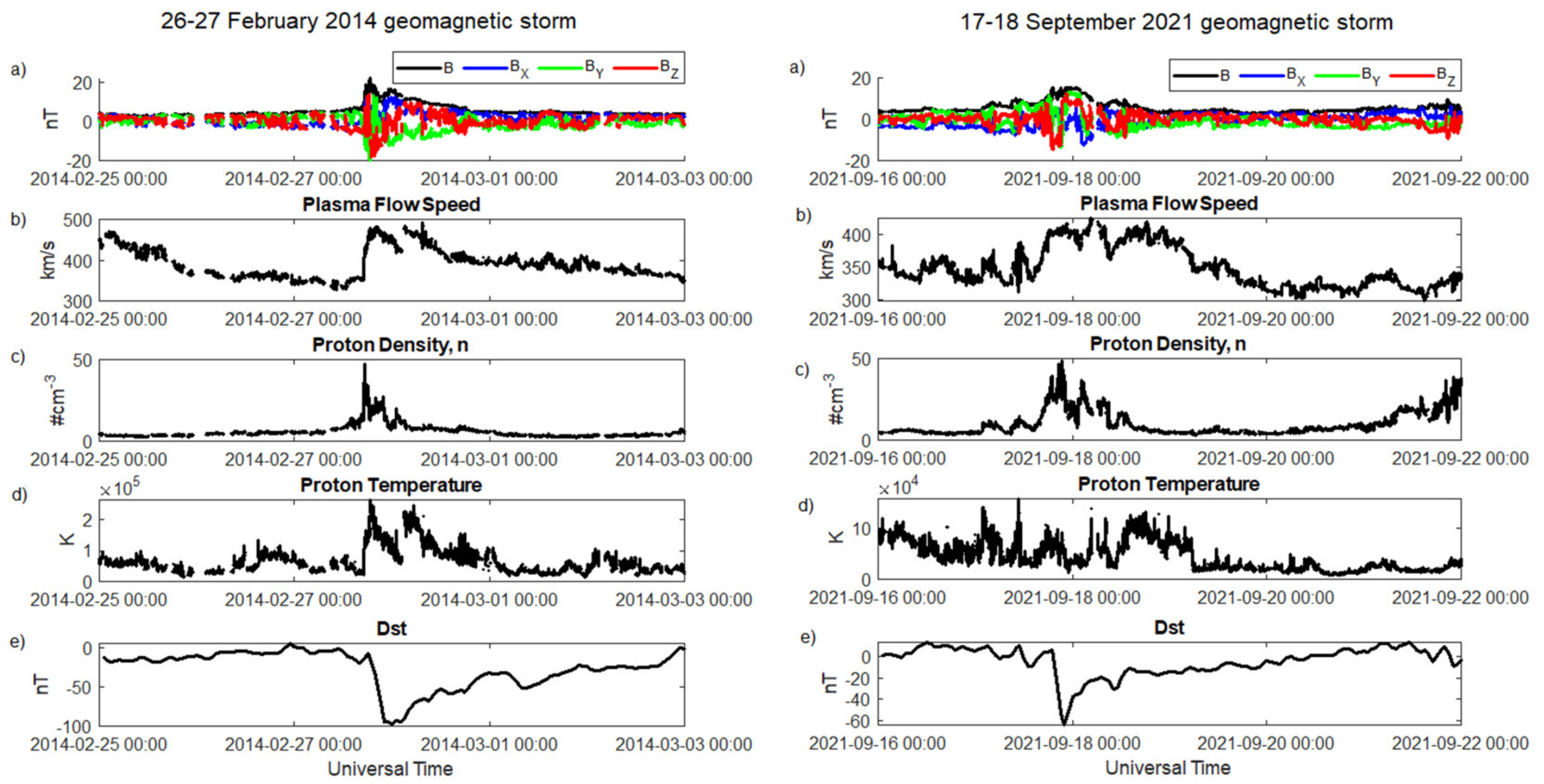
Abstract
1. Introduction
2. Materials and Methods
2.1. Geomagnetic Storms
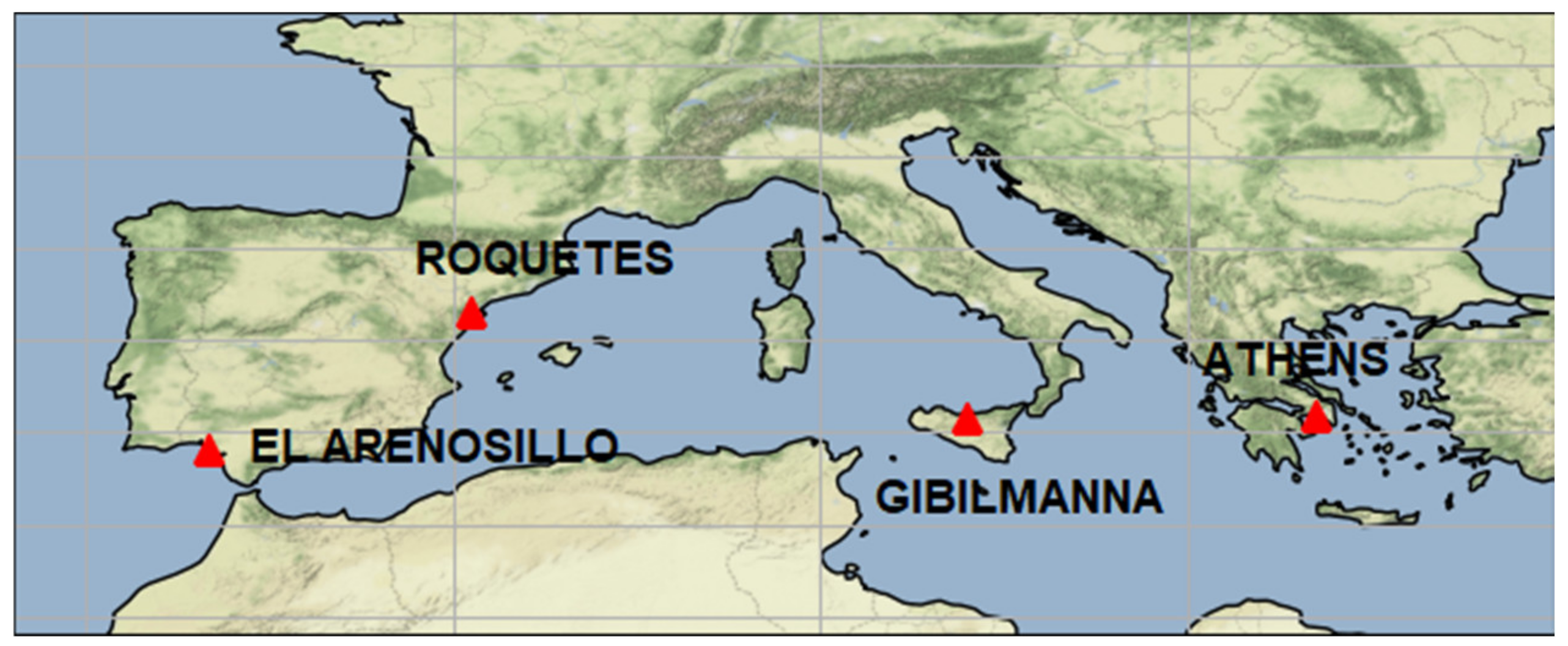
2.2. Ionosonde Data
2.3. TEC Data
2.4. GIMs
3. Results
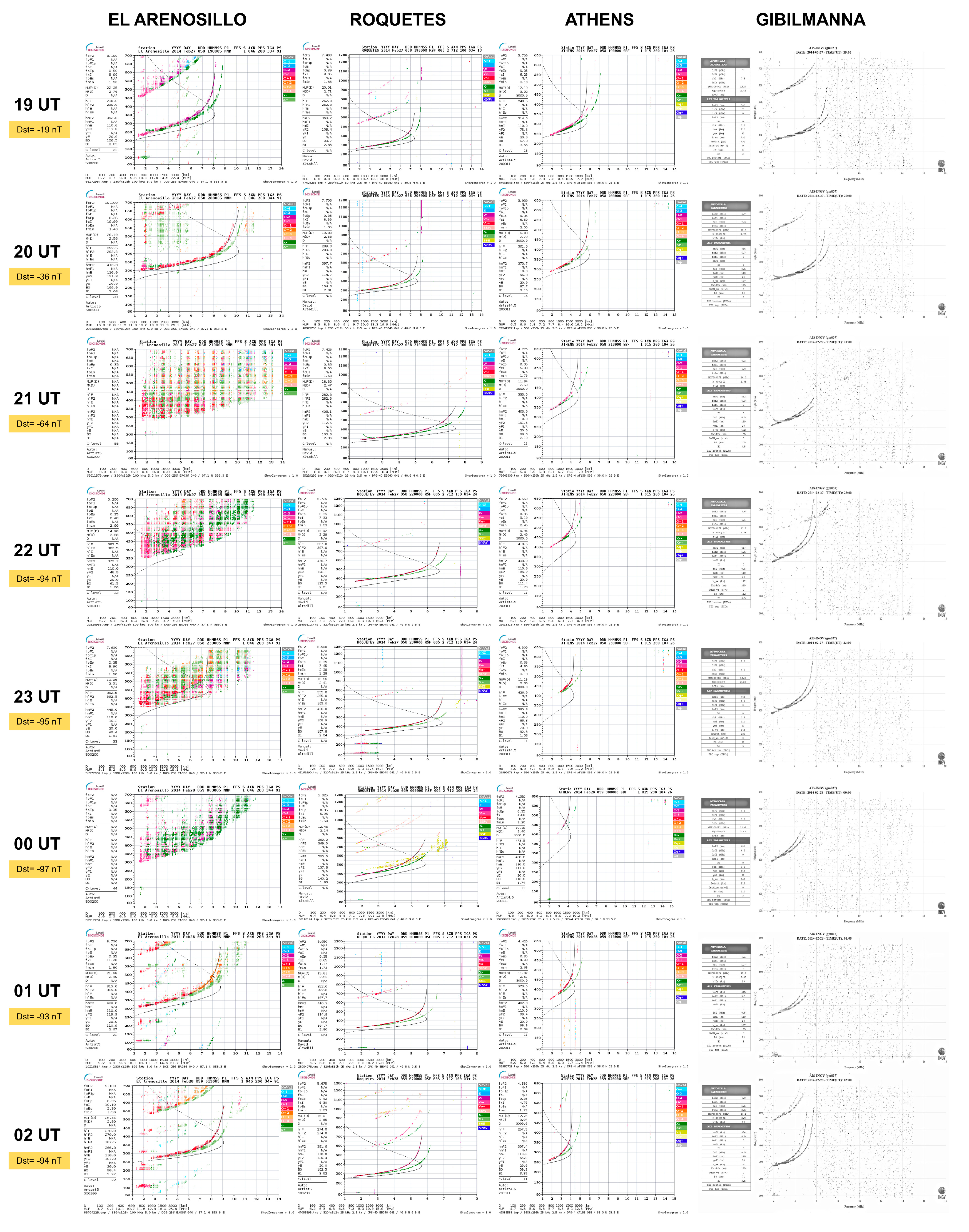
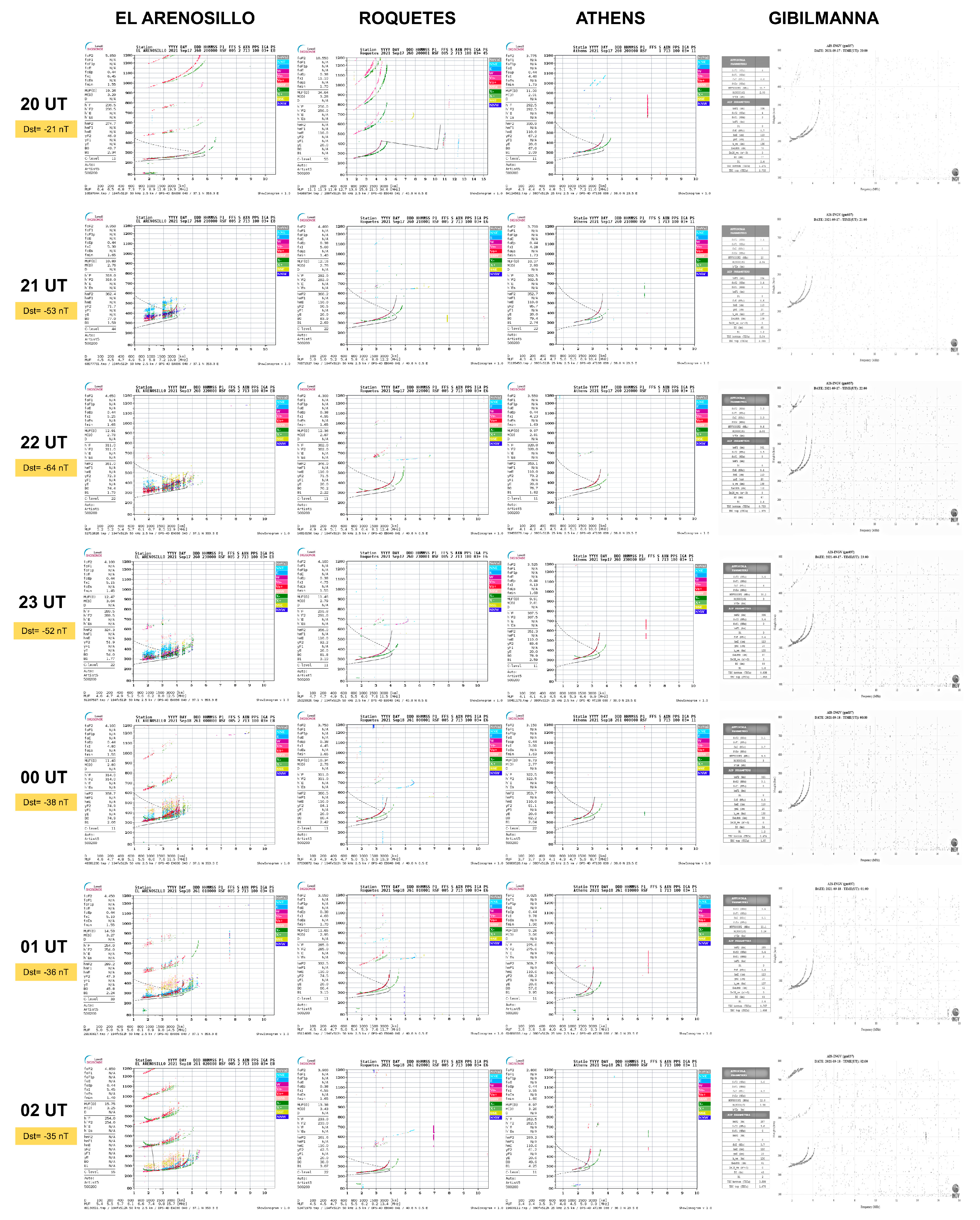
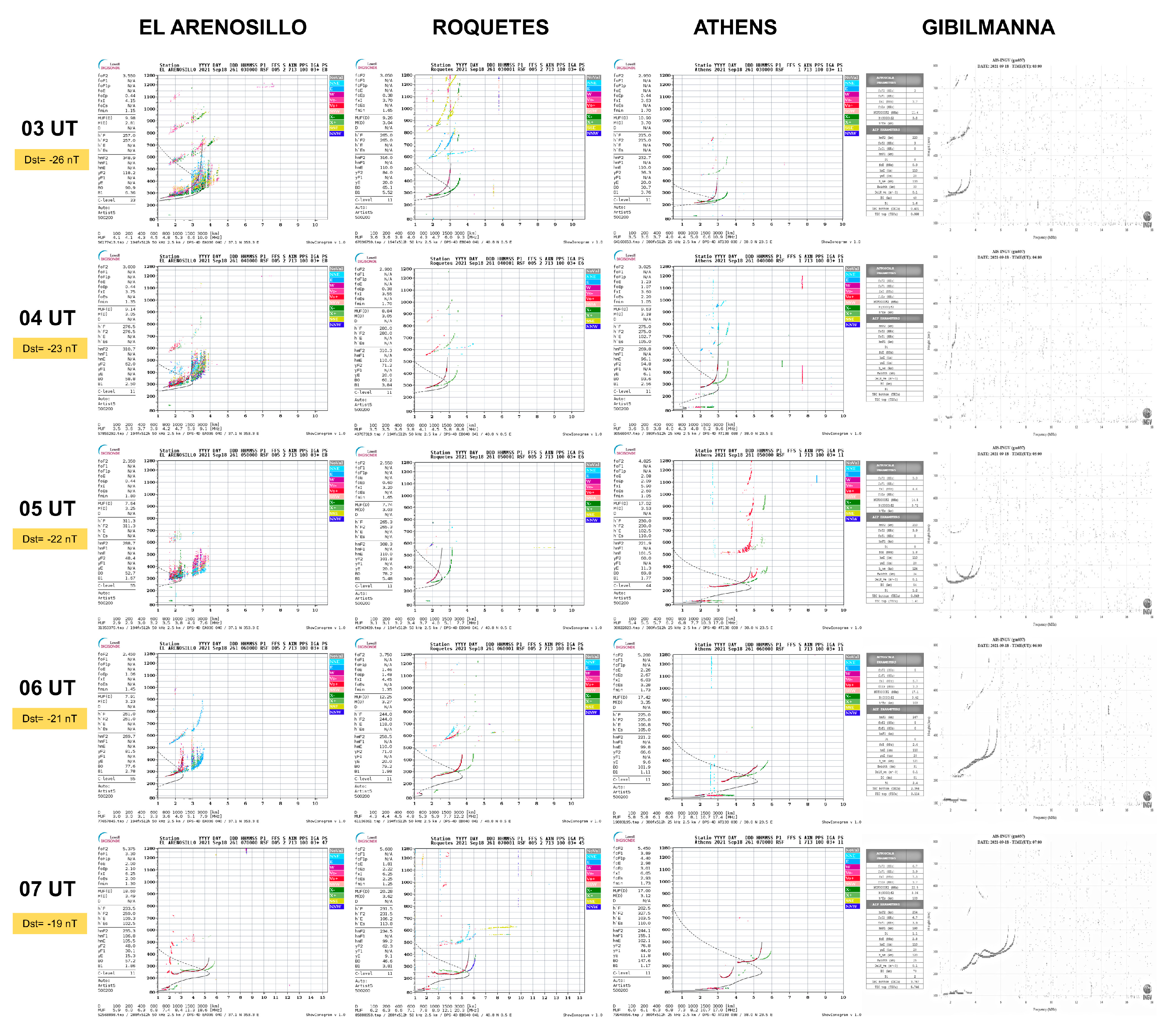
3.1. Ionosonde Results
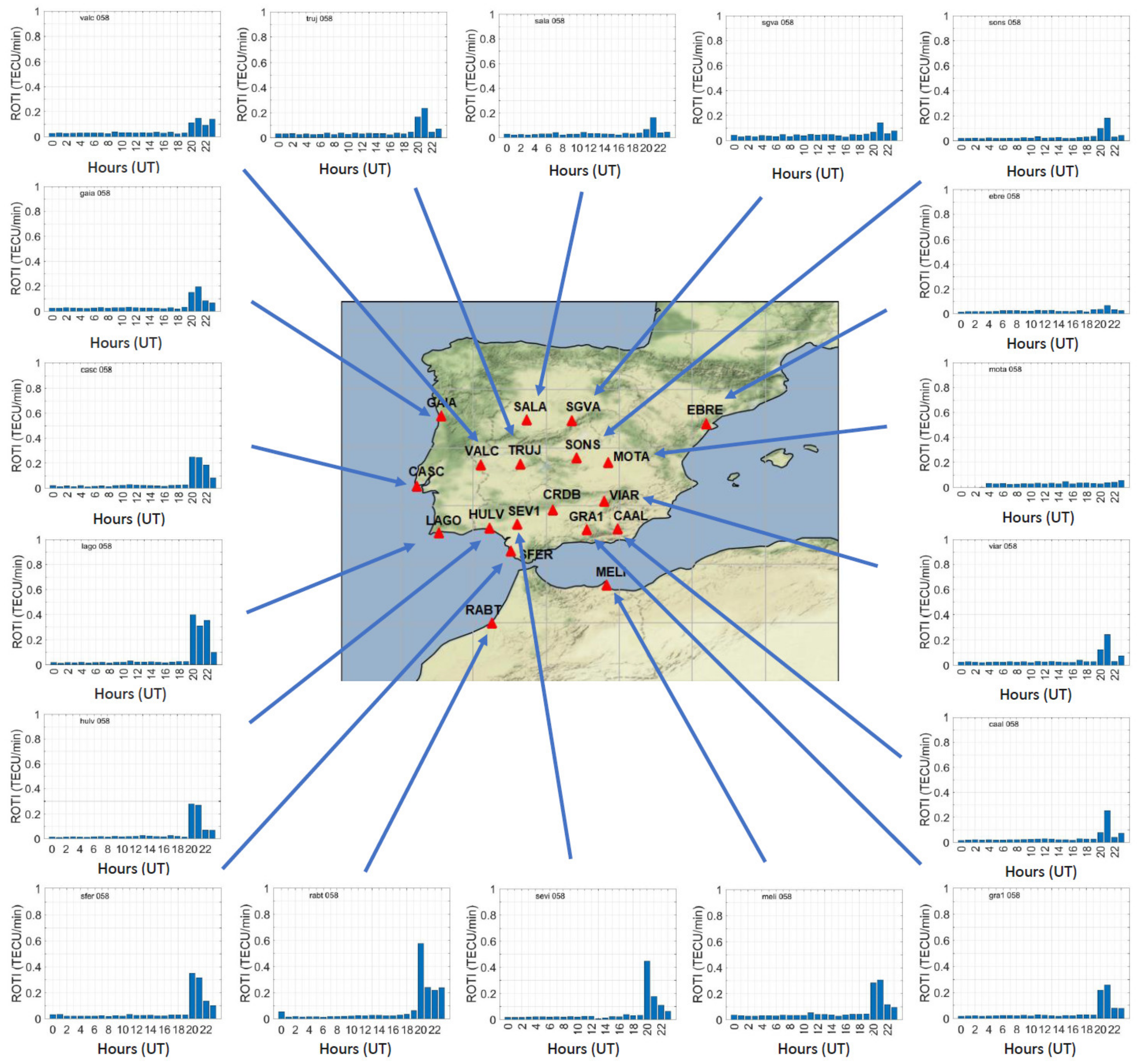
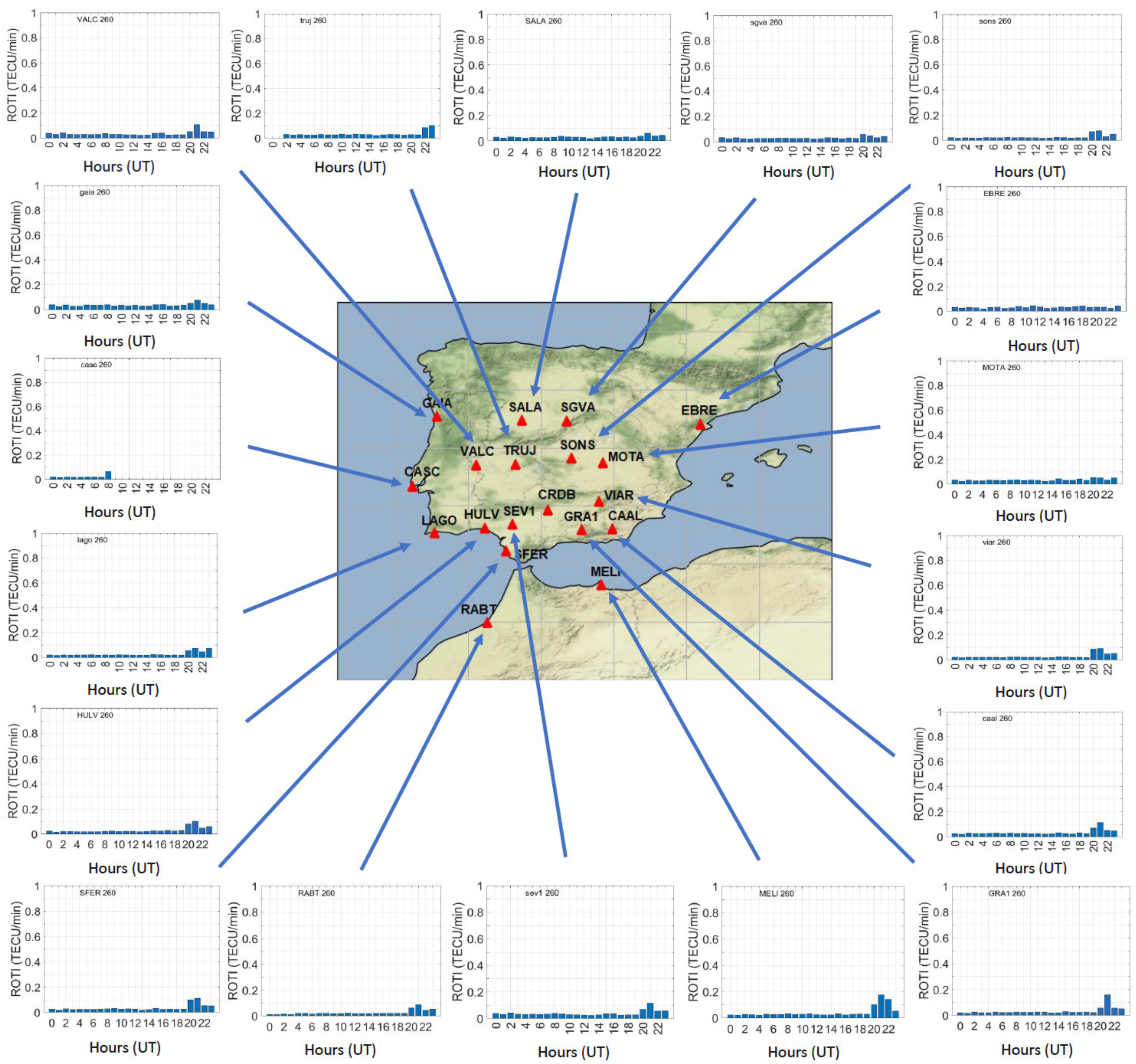
3.2. TEC Results and ROTI
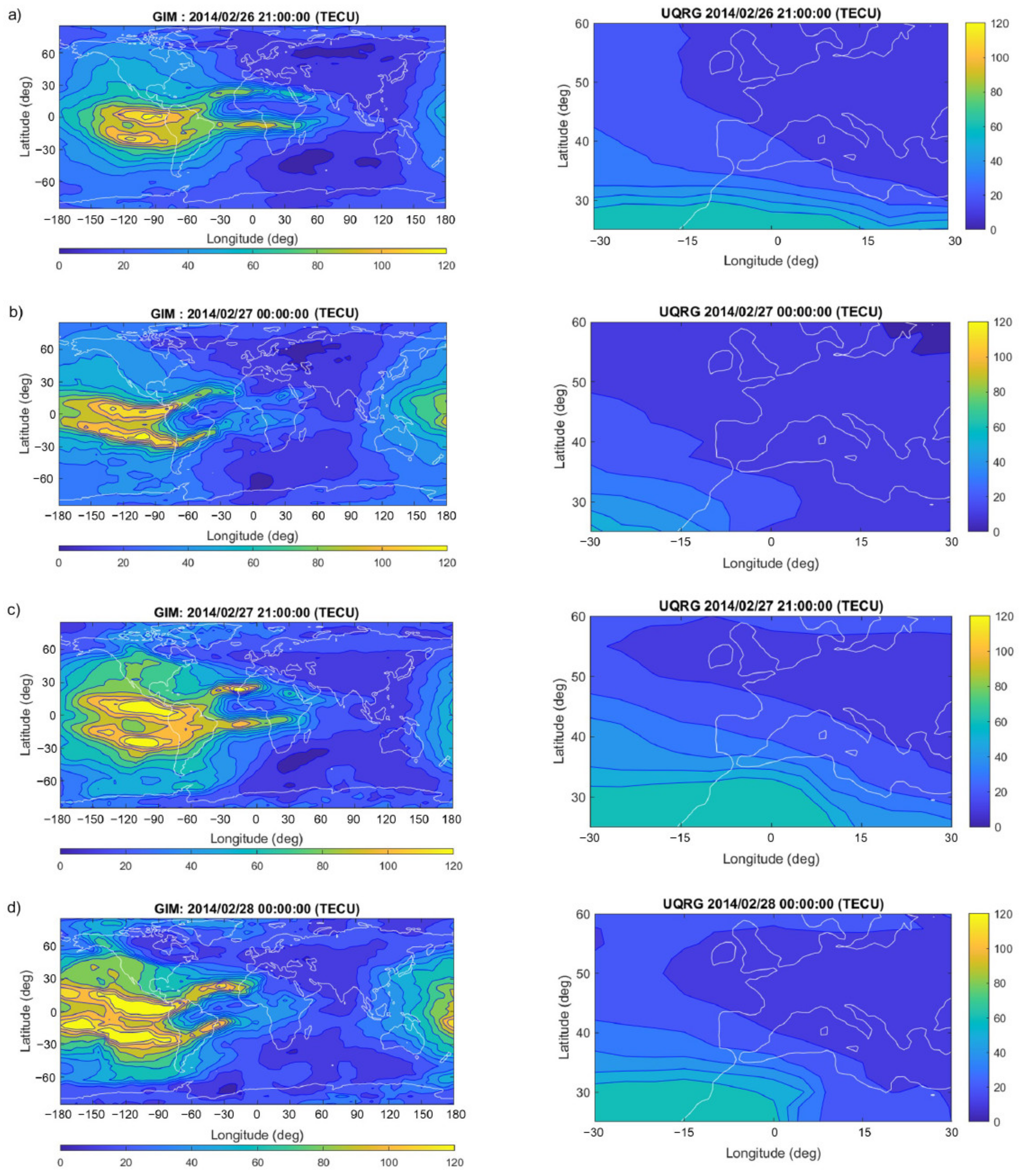
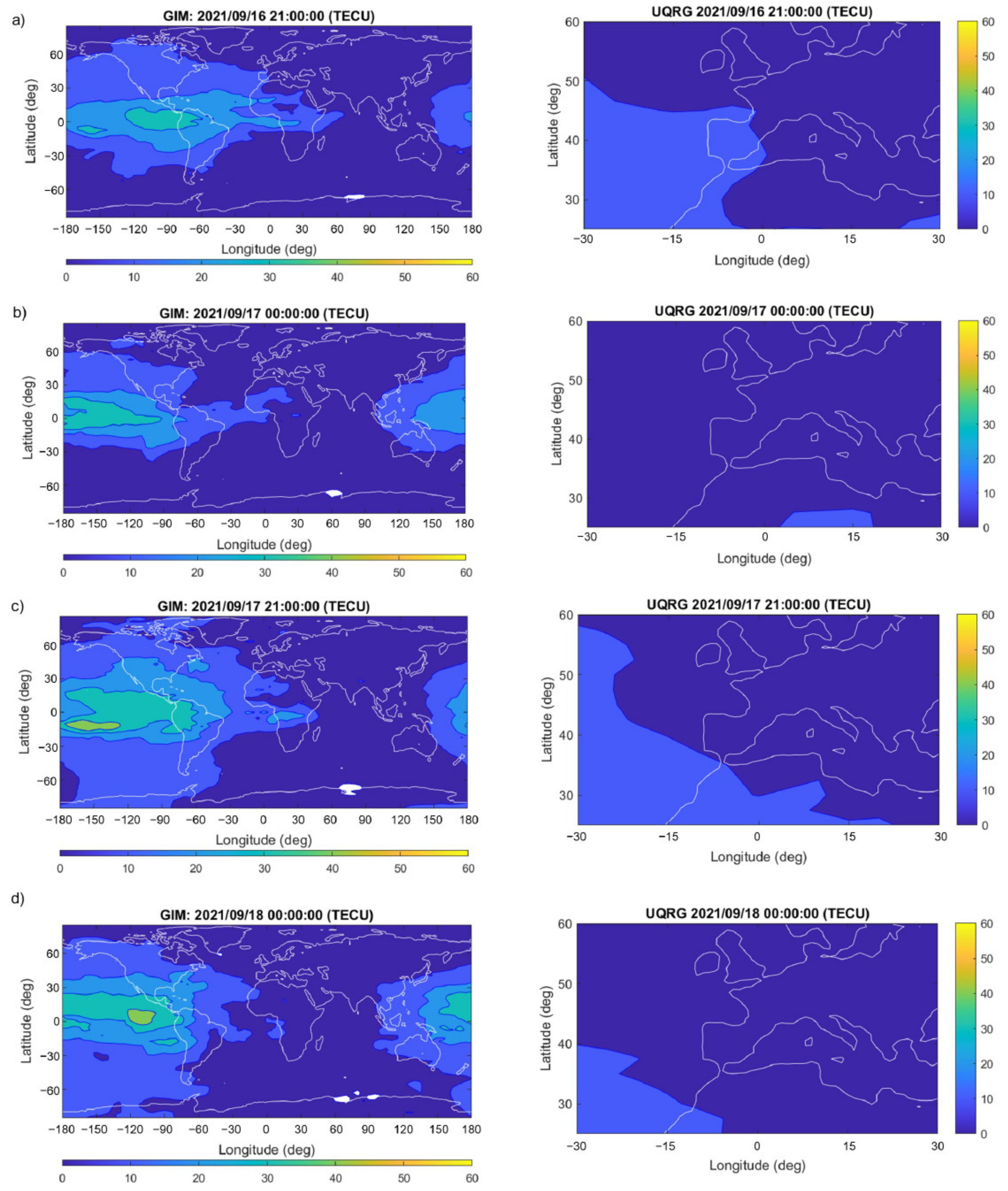
3.3. GIMs
4. Discussion
5. Conclusions
Supplementary Materials
Author Contributions
Funding
Institutional Review Board Statement
Informed Consent Statement
Data Availability Statement
Acknowledgments
Conflicts of Interest
References
- Aarons, J. The longitudinal morphology of equatorial F-layer irregularities relevant to their occurrence. Space Sci. Rev. 1993, 63, 209–243. [Google Scholar] [CrossRef]
- Booker, H.G.; Wells, H.W. Scattering of radio waves by the F-region of the ionosphere. J. Geophys. Res. 1938, 43, 249–256. [Google Scholar] [CrossRef]
- Lan, T.; Jiang, C.; Yang, G.; Sun, F.; Xu, Z.; Liu, Z. Latitudinal Differences in Spread F Characteristics at Asian Longitude Sector during the Descending Phase of the 24th Solar Cycle. Universe 2022, 8, 485. [Google Scholar] [CrossRef]
- Alfonsi, L.; Spogli, L.; Pezzopane, M.; Romano, V.; Zuccheretti, E.; De Franceschi, G.; Cabrera, M.A.; Ezquer, R.G. Comparative analysis of spread-F signature and GPS scintillation occurrences at Tucumán, Argentina. J. Geophys. Res. Space Phys. 2013, 118, 4483–4502. [Google Scholar] [CrossRef]
- Woodman, R.F.; La Hoz, C. Radar observations of F region equatorial irregularities. J. Geophys. Res. 1976, 81, 5447–5466. [Google Scholar] [CrossRef]
- Weber, E.J.; Buchau, J.; Eather, R.H.; Mende, S.B. North-south aligned equatorial airglow depletions. J. Geophys. Res. Space Phys. 1978, 83, 712–716. [Google Scholar] [CrossRef]
- Booker, H.G. Turbulence in the ionosphere with applications to meteor-trails, radio-star scintillation, auroral radar echoes, and other phenomena. J. Geophys. Res. 1956, 61, 673–705. [Google Scholar] [CrossRef]
- Aarons, J.; Mendillo, M.; Yantosca, R.; Kudeki, E. GPS phase fluctuations in the equatorial region during the MISETA 1994 campaign. J. Geophys. Res. Space Phys. 1996, 101, 26851–26862. [Google Scholar] [CrossRef]
- Pi, X.; Mannucci, A.J.; Lindqwister, U.J.; Ho, C.M. Monitoring of global ionospheric irregularities using the worldwide GPS network. Geophys. Res. Lett. 1997, 24, 2283–2286. [Google Scholar] [CrossRef]
- Abe, O.E.; Rabiu, A.B.; Radicella, S.M. Longitudinal Asymmetry of the Occurrence of the Plasma Irregularities over African Low-Latitude Region. Pure Appl. Geophys. 2018, 175, 4355–4370. [Google Scholar] [CrossRef]
- Thanh, D.N.; Le Huy, M.; Amory-Mazaudier, C.; Fleury, R.; Saito, S.; Chien, T.N.; Thi Thu, H.P.; Le Truong, T.; Thi, M.N. Characterization of ionospheric irregularities over Vietnam and adjacent region for the 2008-2018 period. Vietnam. J. Earth Sci. 2021, 43, 1–20. [Google Scholar] [CrossRef]
- Balan, N.; Liu, L.; Le, H. A brief review of equatorial ionization anomaly and ionospheric irregularities. EPP 2018, 2, 257–275. [Google Scholar] [CrossRef]
- Migoya-Orué, Y.O.; Radicella, S.M.; Coïsson, P. Low latitude ionospheric effects of major geomagnetic storms observed using TOPEX TEC data. Ann. Geophys. 2009, 27, 3133–3139. [Google Scholar] [CrossRef]
- Abdu, M.A. Major phenomena of the equatorial ionosphere thermosphere system under disturbed conditions. J. Atmos. Solar Terr. Phys. 1997, 59, 1505–1519. [Google Scholar] [CrossRef]
- Tanaka, T. Low-latitude ionospheric disturbances: Results for March 22, 1979, and their general characteristics. Geophys. Res. Lett. 1986, 13, 1399–1402. [Google Scholar] [CrossRef]
- Lin, C.H.; Richmond, A.D.; Heelis, R.A.; Bailey, G.J.; Lu, G.; Liu, J.Y.; Yeh, H.C.; Su, S.-Y. Theoretical study of the low- and midlatitude ionospheric electron density enhancement during the October 2003 superstorm: Relative importance of the neutral wind and the electric field. J. Geophys. Res. 2005, 110, A12312. [Google Scholar] [CrossRef]
- Cherniak, I.; Zakharenkova, I. First observations of super plasma bubbles in Europe. Geophys. Res. Lett. 2016, 43, 137–145. [Google Scholar] [CrossRef]
- Kashcheyev, A.; Migoya-Orué, Y.; Amory-Mazaudier, C.; Fleury, R.; Nava, B.; Alazo-Cuartas, K.; Radicella, S.M. Multivariable comprehensive analysis of two great geomagnetic storms of 2015. J. Geophys. Res. Space Phys. 2018, 123, 5000–5018. [Google Scholar] [CrossRef]
- Azzouzi, I.; Migoya-Orue, Y.; Amory Mazaudier, C.; Fleury, R.; Radicella, S.M.; Touzani, A. Signatures of solar event at middle and low latitudes in the Europe-African sector, during geomagnetic storms, October 2013. Adv. Space Res. 2015, 56, 2040–2055. [Google Scholar] [CrossRef]
- Orús, R.; Hernández-Pajares, M.; Juan, J.; Sanz, J. Improvement of global ionospheric VTEC maps by using kriging interpolation technique. J. Atmos. Sol.-Terr. Phys. 2005, 67, 1598–1609. [Google Scholar] [CrossRef]
- Sur, D.; Hammou Ali, O.; Binti Sarudin, I.; Rupiewicz, J.; Bravo, M.; Toriashvili, L.; Sun, X. Effects of Geomagnetic Storm on Equatorial Ionization during 27 February–1 March, 2014. In Proceedings of the AGU Fall Meeting 2018, Washington, DC, USA, 10–14 December 2018. [Google Scholar]
- SpaceWeather.com. Available online: https://www.spaceweather.com/archive.php?view=1&day=17&month=09&year=2021 (accessed on 11 October 2022).
- Ciraolo, L.; Azpilicueta, F.; Brunini, C.; Meza, A.; Radicella, S.M. Calibration errors on experimental slant total electron content (TEC) determined with GPS. J. Geod. 2007, 81, 111–120. [Google Scholar] [CrossRef]
- Hernández-Pajares, M.; Juan, J.M.; Sanz, J.; Orus, R.; Garcia-Rigo, A.; Feltens, J.; Komjathy, A.; Schaer, S.C.; Krankowski, A. The IGS VTEC maps: A reliable source of ionospheric information since 1998. J. Geod. 2009, 83, 263–275. [Google Scholar] [CrossRef]
- Malki, K.; Bounhir, A.; Benkhaldoun, Z.; Makela, J.J.; Vilmer, N.; Fisher, D.J.; Kaab, M.; Elbouyahyaoui, K.; Harding, B.J.; Laghriyeb, A.; et al. Ionospheric and thermospheric response to the 27–28 February 2014 geomagnetic storm over north Africa. Ann. Geophys. 2018, 36, 987–998. [Google Scholar] [CrossRef]
- Basu, S.; Kelly, M.C. Review of equatorial scintillation phenomena in light of recent developments in the theory and measurement of equatorial irregularities. J. Atmos. Terr. Phys. 1977, 39, 1229–1247. [Google Scholar] [CrossRef]
- Fejer, B.G.; Scherliess, L.; de Paula, E.R. Effects of the vertical plasma drift velocity on the generation and evolution of equatorial spread F. J. Geophys. Res. 1999, 104, 19859–19869. [Google Scholar] [CrossRef]
- Magdaleno, S.; Herraiz, M.; Altadill, D.; de la Morena, B.A. Climatology characterization of equatorial plasma bubbles using GPS data. J. Space Weather Space Clim. 2017, 7, A3. [Google Scholar] [CrossRef]
- Sripathi, S.; Sreekumar, S.; Banola, S. Characteristics of equatorial and low-latitude plasma irregularities as investigated using a meridional chain of radio experiments over India. J. Geophys. Res. Space Phys. 2018, 123, 4364–4380. [Google Scholar] [CrossRef]
- Shi, J.K.; Wang, G.J.; Reinisch, B.W.; Shang, S.P.; Wang, X.; Zherebotsov, G.; Potekhin, A. Relationship between strong range spread F and ionospheric scintillations observed in Hainan from 2003 to 2007. J. Geophys. Res. 2011, 116, A08306. [Google Scholar] [CrossRef]
- Paul, K.S.; Haralambous, H.; Oikonomou, C.; Paul, A.; Belehaki, A.; Ioanna, T.; Kouba, D.; Buresova, D. Multi-station investigation of spread F over Europe during low to high solar activity. J. Space Weather Space Clim. 2018, 8, A27. [Google Scholar] [CrossRef]
- Dungey, J.W. Convective diffusion in the equatorial F region. J. Atmos. Terr. Phys. 1956, 9, 304–310. [Google Scholar] [CrossRef]
- Perkins, F. Spread F and ionospheric currents. J. Geophys. Res. 1973, 78, 218–226. [Google Scholar] [CrossRef]
- Cherniak, I.; Zakharenkova, I. Development of the storm-induced ionospheric irregularities at equatorial and middle latitudes during the 25–26 August 2018 major geomagnetic storm. Space Weather 2022, 20, e2021SW002891. [Google Scholar] [CrossRef]


Disclaimer/Publisher’s Note: The statements, opinions and data contained in all publications are solely those of the individual author(s) and contributor(s) and not of MDPI and/or the editor(s). MDPI and/or the editor(s) disclaim responsibility for any injury to people or property resulting from any ideas, methods, instructions or products referred to in the content. |
© 2023 by the authors. Licensee MDPI, Basel, Switzerland. This article is an open access article distributed under the terms and conditions of the Creative Commons Attribution (CC BY) license (https://creativecommons.org/licenses/by/4.0/).
Share and Cite
Campuzano, S.A.; Delgado-Gómez, F.; Migoya-Orué, Y.; Rodríguez-Caderot, G.; Herraiz-Sarachaga, M.; Radicella, S.M. Study of Ionosphere Irregularities over the Iberian Peninsula during Two Moderate Geomagnetic Storms Using GNSS and Ionosonde Observations. Atmosphere 2023, 14, 233. https://doi.org/10.3390/atmos14020233
Campuzano SA, Delgado-Gómez F, Migoya-Orué Y, Rodríguez-Caderot G, Herraiz-Sarachaga M, Radicella SM. Study of Ionosphere Irregularities over the Iberian Peninsula during Two Moderate Geomagnetic Storms Using GNSS and Ionosonde Observations. Atmosphere. 2023; 14(2):233. https://doi.org/10.3390/atmos14020233
Chicago/Turabian StyleCampuzano, Saioa A., Fernando Delgado-Gómez, Yenca Migoya-Orué, Gracia Rodríguez-Caderot, Miguel Herraiz-Sarachaga, and Sandro M. Radicella. 2023. "Study of Ionosphere Irregularities over the Iberian Peninsula during Two Moderate Geomagnetic Storms Using GNSS and Ionosonde Observations" Atmosphere 14, no. 2: 233. https://doi.org/10.3390/atmos14020233
APA StyleCampuzano, S. A., Delgado-Gómez, F., Migoya-Orué, Y., Rodríguez-Caderot, G., Herraiz-Sarachaga, M., & Radicella, S. M. (2023). Study of Ionosphere Irregularities over the Iberian Peninsula during Two Moderate Geomagnetic Storms Using GNSS and Ionosonde Observations. Atmosphere, 14(2), 233. https://doi.org/10.3390/atmos14020233