Article

A Low-Cost Calibration Method for Temperature, Relative Humidity, and Carbon Dioxide Sensors Used in Air Quality Monitoring Systems

by
Rosa Amalia González Rivero
1,
Luis Ernesto Morera Hernández
1,
Olivier Schalm
2,*,
Erik Hernández Rodríguez
1,
Daniellys Alejo Sánchez
1,
Mayra C. Morales Pérez
1,
Vladimir Nuñez Caraballo
3,
Werner Jacobs
2 and
Alain Martinez Laguardia
1
1
Department of Chemistry, Universidad Central “Marta Abreu” de Las Villas, Road to Camajuaní Km 5.5, Santa Clara 54830, Villa Clara, Cuba
2
Antwerp Maritime Academy, Noordkasteel Oost 6, 2030 Antwerpen, Belgium
3
Meteorological Center, Marta Abreu Street, Santa Clara 50100, Villa Clara, Cuba
*
Author to whom correspondence should be addressed.
Atmosphere 2023, 14(2), 191; https://doi.org/10.3390/atmos14020191
Submission received: 22 December 2022 / Revised: 8 January 2023 / Accepted: 10 January 2023 / Published: 17 January 2023

Abstract

:
Low-cost sensors provide an affordable alternative to monitor environmental parameters with acceptable performance. There is a substantial amount of literature where low-cost sensors are compared with high-end reference measurements. However, not all organizations have access to such reference infrastructure. We propose low-cost calibration methods for temperature, relative humidity, and CO2 to allow them to collect their own reliable data. These methods are based on simple techniques and procedures that allow temperature calibration to be achieved in the range of 0 to 50 °C, relative humidity from 0 to 90%, and CO2 between 0 and 1100 ppm. The materials used to create the calibration setups can be purchased online, at hardware stores, and in pharmacies. The reliability of the calibration methods was evaluated using several indicators, such as the airtightness of the calibration box, similarity with the factory calibration, similarity with the reference, similarity between different sensors, replicability of the calibration method, and the similarity with a golden standard. In addition, the results of the low-cost calibration methods were compared with the more advanced calibration methods. A short measurement campaign in the city of Santa Clara, Cuba, demonstrated that such calibrations transform in-house developed monitoring systems into valid low-cost scientific instruments for decision-making. This work creates opportunities for institutions and researchers hosted in low- and mid-income countries to build and validate their own equipment to reliably solve local problems.

1. Introduction

Due to the increase in anthropogenic emissions of pollutants into the atmosphere, the evaluation of ambient air quality has become an important environmental concern during the last decades [1,2,3,4,5]. Many countries have a network of reference monitoring stations that measure air quality in real time. However, the high installation and maintenance costs of these stations mean that low- and middle-income countries are less covered by such stations. In those regions, alternative technologies such as low-cost monitoring systems can be used instead [6,7,8,9,10]. Some define a low-cost sensor as <$100 and a low-cost monitor consisting of one or more sensors and communication/data components as <$1000 [11]. The need for low-cost monitoring devices also exists in specific sectors in high-income countries. For example, temperature (T) and relative humidity (RH) monitoring in museums, archives, or churches are critical to assess the aggressiveness of ambient air toward heritage objects [12,13,14,15]. Unfortunately, investments in measuring instruments are frequently limited by the available budgets [16]. Another example is the reduction of the risk of losing expensive instruments by attaching low-cost devices (e.g., the Ozonesonde) to a weather balloon for measuring environmental parameters at high altitudes [17,18]. With the low-cost open hardware technology that exists on the market, citizens and pupils can build their own monitoring systems to measure the local air quality of their interest [19]. Several citizen science platforms such as Sensor. Community or PurpleAir are currently used in research [20,21,22,23].
Scientific literature regarding the use of low-cost sensors is growing. A search in the database of ScienceDirect resulted in around 500 hits for 2021 when using the keyword “low-cost sensor”, including several reviews [24,25,26,27,28,29]. It is striking that quite a few publications emphasize the (calibration) limitations and the performance problems of such sensors [30,31,32]. These studies demonstrate that such sensors do not achieve the same data quality as obtained by reference methods, which is to be expected. In contrast to this negative way of evaluating low-cost sensors, one can also evaluate the possibilities of such technology and show how they can be used to build low-cost scientific instruments that are good enough to evaluate air quality [33]. Sensors and calibrations are complementary and equally important. The search for literature in ScienceDirect using the term “low-cost calibration” resulted in only four hits for 2021, and only one was related to air quality [34]. This suggests that the popularity of comparing low-cost sensors with state-of-the-art technology is higher than the development of low-cost calibration methods for low-cost sensors. This work aims to develop low-cost calibration methods so that institutes or areas without access to high-end equipment can perform their own reliable measurement campaigns.
The calibration of low-cost sensors with state-of-the-art reference instruments and the calibration of low-cost sensors with low-cost calibration methods correspond to the distinction between maximizers and satisficers [35]. A maximizer is someone who wants only the very best and who strives to make a choice that will give them the maximum benefit later on. One evaluates all possible options before one makes a decision. A satisficer is someone who makes a decision or takes action as soon as an option meets his criteria. Once one has found the option that is good enough, one stops his quest for better alternatives. A satisficer does not necessarily settle for mediocrity. His criteria can be very high, but as soon as one finds a low-cost scientific instrument that has the qualities he wants, one is satisfied. What he wants is an air quality monitoring system at a low-cost with high reliability that provides data that can be used by decision-makers who are responsible for improving the air quality. To obtain such a system, the satisficer can enhance the reliability of the monitoring system with a restricted budget by suppressing noise or removing spikes in the acquired data using data processing techniques. Another way to improve the data quality is to calibrate the sensors with low-cost methods. However, such calibration methods have been rarely mentioned in the literature.
A maximizer will only be satisfied when one can perform his analyses with the best possible measuring instruments that are available on the market [36]. When one is obliged to use low-cost sensors, one will strive for sensor calibration using state-of-the-art technology. He will compare sensors with reference measurements in laboratory conditions where environmental parameters are changed in a controlled way [37,38]. An alternative comparative test is to perform co-location experiments near national air quality measuring stations, where pollutants in the air are determined with sufficient accuracy [20,39,40]. Reference instruments can also be built inside a van to make them mobile so that co-location experiments can be performed at any location that is needed [41,42]. Different kinds of calibration procedures are applied to the parallel measurements performed in a laboratory or in co-location [9,28,43]: simple linear regression, multi-linear regression [44], or machine learning [10,45,46] methods. A drawback of the maximizer’s methods is that his way of working is impossible when one has no access to high-end equipment. In addition, the advantages of low-cost sensors decrease when expensive calibration methods are required.
This contribution focuses on the satisficer’s way of thinking, where data quality obtained by low-cost sensors is improved without the aid of expensive state-of-the art equipment. For example, the T inside a closed box can easily be manipulated using a heater or a Peltier cooler, while a simple glass thermometer acts as the reference device. The RH in a sealed container can be changed in a controlled way using saturated salt solutions [16,47,48,49,50,51,52,53,54]. An alternative method to control the RH is with glycerol solutions [55,56,57,58,59,60], which appear to be more convenient because one product can generate any kind of RH. For CO2, methods to generate small but known amounts of gas using disposable medical equipment, such as plastic syringes, have been reported [61]. The setup proposed in this contribution can also be used to generate NO2 and SO2 in small but known amounts [62]. For gaseous pollutants, ambient air analyzed with classical methods of wet chemistry analysis, such as titrations [63], turbidity [64], colorimetry [65,66,67,68], or fluorimetry [69], can be used as a reference measurement. In addition, several indicators (e.g., airtightness of the closed box) are defined, which gives an insight into the reliability of the calibration methods. Further to the development of low-cost calibration methods for T, RH, and CO2, the usefulness of the calibration methods is illustrated in a case study where these parameters were monitored at several locations in the city of Santa Clara, Cuba. The measurement campaigns illustrate that in-house developed monitoring systems can be used to generate reliable and useful data without the need for expensive reference measurement devices, even when the quality of the collected data is most probably lower than that of reference instruments.

2. Materials and Methods

2.1. Sensors Used with the Low-Cost Monitoring System

The low-cost monitoring system that was used in the experiments consisted of an Arduino MEGA2560 (provided by Tinytronics, Eindhoven, The Netherlands) as the computer unit and interface board, a real-time clock, and an SD-card for data storage. The total price of the monitoring system was below €200. More information about the monitoring system can be found elsewhere [70,71,72]. Different sensors were coupled to the monitoring system during the calibration experiments (see Table 1). To distinguish the five different AM2315 sensors (provided by Tinytronics, Eindhoven, The Netherlands) that were used, a number was attributed to them.

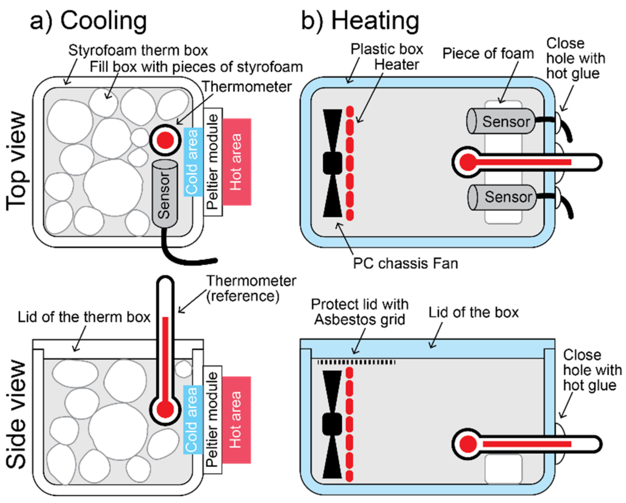
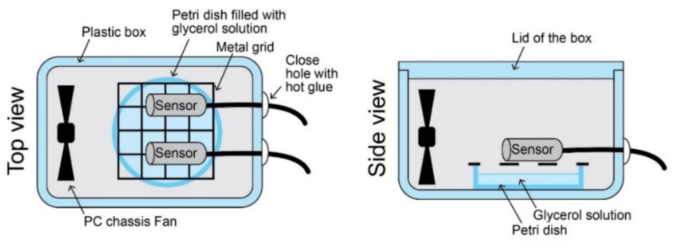
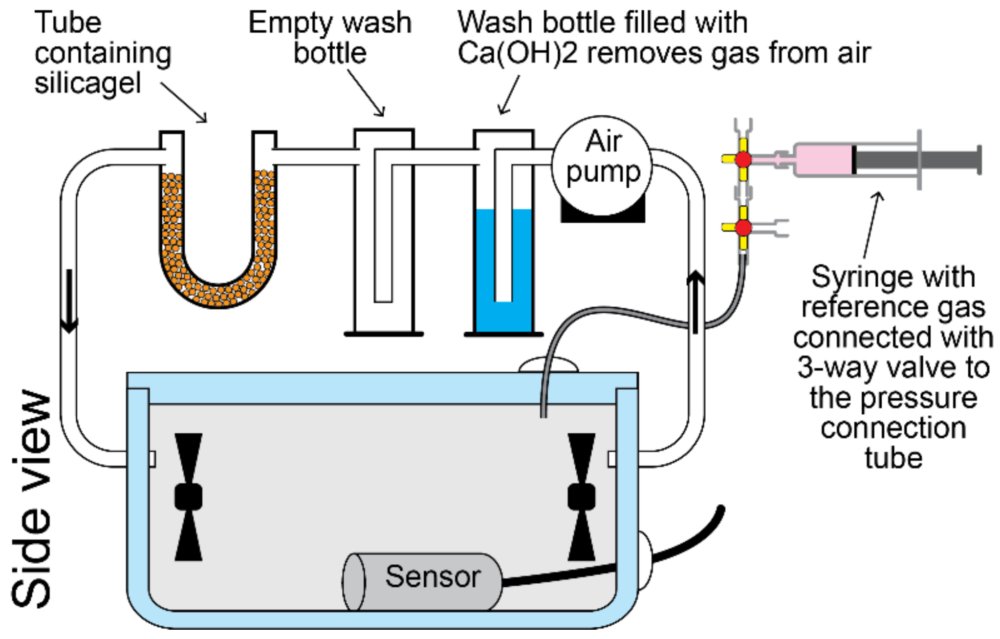
2.2. Design of a Low-Calibration Laboratory

A low-cost calibration laboratory that can evaluate T, RH, and gas (i.e., CO2, but other gasses such as NO2 or SO2 are also possible with the setup) requires an investment between €1000 and €1500. The prices mentioned in Table 2 are per individual item, but in some cases, the items can only be purchased in larger boxes (e.g., syringes). Other items such as the plastic box can be used in other calibration setups. Medical disposables were also reused several times. It should be noted that the low-cost calibration methods are more labor-intensive. How the items were used to build the calibration setups are shown in Figure 1, Figure 2, Figure 3 and Figure 4.

2.3. Temperature Calibration

Several calibration experiments were performed in a laboratory located in Santa Clara, Cuba. For these experiments, the average air T and RH were 27 °C and 64%. The calibration of the T parameter of the AM2315 sensors was performed in two stages: (1) the cooling of the ambient air inside a Styrofoam box filled with smaller pieces of Styrofoam, leaving only a small volume for the sensors and the reference glass thermometer (Figure 1a) using a Peltier cooler so that the T decreases from room T (26 °C) down to 0 °C; and (2) the heating of ambient air in a closed plastic box (Figure 1b) by placing a mica heater inside the box that is coupled to a thermostat so that the T rises from room T to 50 °C. A glass thermometer acts as a reference device to measure the T inside the box. During the experiment, the sensor readings were registered by the low-cost data logger. Meanwhile, the T of the glass thermometer was visually determined and their values were written down with the corresponding timestamp in a laboratory notebook. Both time series were merged by selecting the sensor reading with the same timestamp as the measured value of the glass thermometer. The calibration curves were determined by processing the data in Microsoft Excel.

2.4. Relative Humidity Calibration

Pure glycerol in a closed box generates a RH of 0%; pure water generates a RH of 100%. The density of the glycerol solution taken from the bottle (Sigma Aldrich, 99%) was determined with a pycnometer (i.e., 1.25960 g/mL) and its density corresponded with a RH of 12.73% (detailed information about the calculations of the corresponding RH can be found in the Supplementary Material). This was the minimum RH in the calibration experiment. Six solutions with glycerol concentrations of 99, 80, 70, 50, 40, and 0 vol% were prepared to perform a series of experiments with increasing RH. The solutions with higher glycerol concentrations resulted in a drying effect of the ambient RH conditions in the calibration box (ambient conditions during the calibration session were about 60–95%); the solution with high water content resulted in humidification. The pure glycerol solution took about 6 h before the RH in the box reached its equilibrium. The time that the calibration box reached equilibrium became shorted with the increasing water content in the mixture.
The experiments were carried out inside a plastic box of 6.27 L closed with a plastic lid. A closed container with a volume larger than 1 L should contain a fan [53]. A Petri dish of 15 cm diameter containing a glycerol solution of 380 mL was placed at the bottom of the box. The Petri dish guarantees a large surface of the solution to allow free diffusion of water. A grid was placed on top of the Petri dish. The sensor was placed on top of that grid. The box also contained two PC chassis fans to assure the homogeneity inside the box and to speed up the moisture exchange between air and glycerol solution so that equilibrium was reached faster (Figure 2). For each experiment, the sensor signal was registered over time and stopped once the signal remained constant for at least 1 h. For the six experiments, the measured and theoretical concentrations determined from the density of the glycerol solutions were brought together in Microsoft Excel to generate the calibration curve.

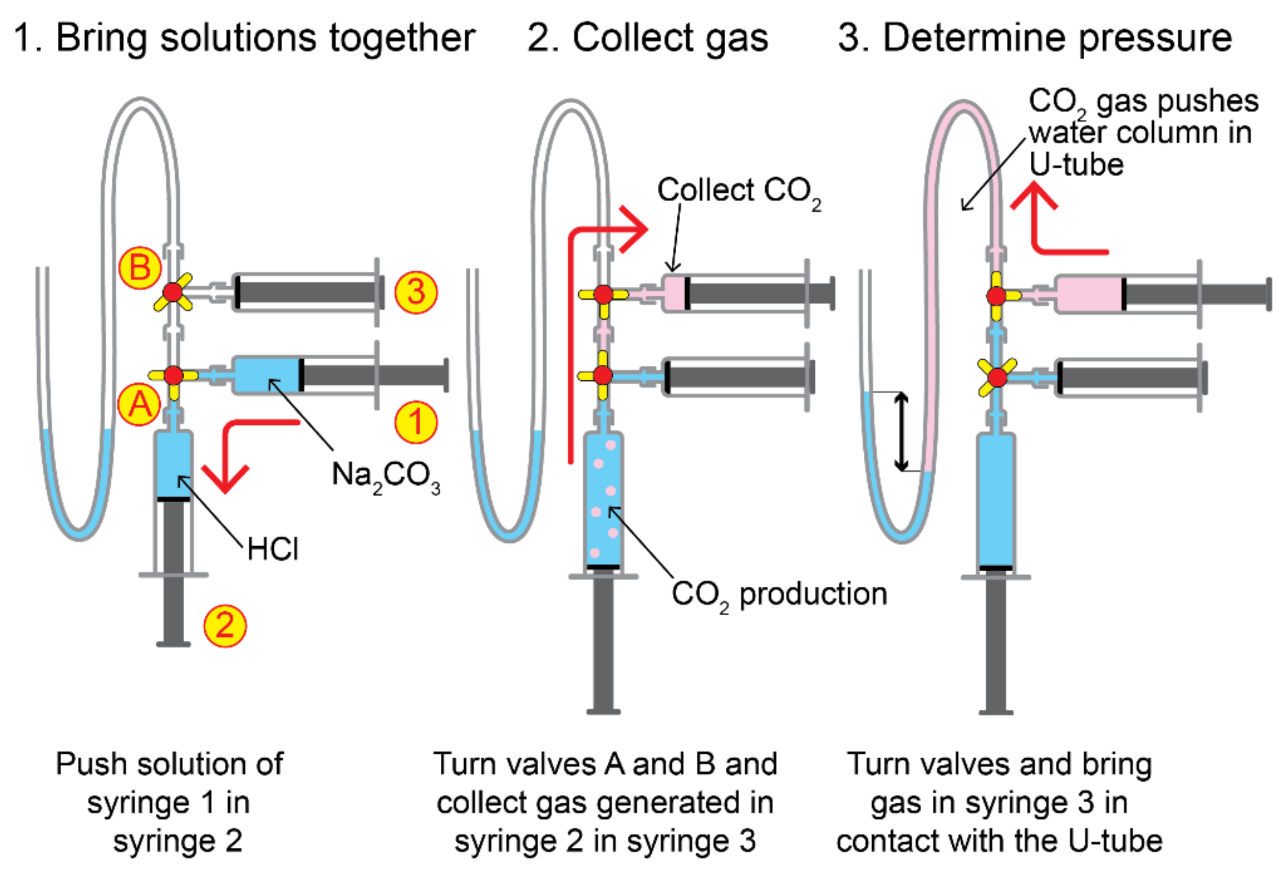
2.5. Calibration of Gas Sensors

The calibration of the gas sensors was performed inside the same plastic box as used in the RH calibration experiment. The box contained two PC chassis fans to homogenize the air inside the calibration box. For CO2, the box contained the appropriate sensor that was coupled to the monitoring device. Before the calibration experiments started, the CO2 concentration in ambient air and also inside the closed box was measured. The box was also coupled to a closed circuit that could remove the CO2 in the ambient air inside the box (see Figure 3). That circuit contained (1) a pump, (2) a wash bottle with 80 mL of saturated Ca(OH)2 solution plus 20 g of NaOH beads that removed CO2 from the air according to reaction (1), (3) an empty wash bottle to trap the water droplets present in air, and (4) a U-shaped glass tube containing 10 g of silica gel to dry the air. The CO2 inside the closed box was removed by switching on the pump. After several minutes, zero air was obtained and the pump was switched off.
Ca OH 2   aq + CO 2   g   CaCO 3   aq + H 2 O
The concept of gas calibration relies on the generation of small but known amounts of gas using stoichiometric reactions [61,73,74,75,76]. The setup used to generate CO2 gas inside a syringe is shown in Figure 4. It was built with low-cost medical disposables, such as Luer Lock syringes, three-way sterile stopcocks, and an extension tube with Luer Lock to create a U tube manometer (see Table 2). Two syringes were used to mix the two reagents mentioned in reaction (2), while the third was used to collect the generated CO2 gas. The volume of CO2 gas can be measured from the tick marks on syringe 3. The T of the gas is equal to the room T and can be measured with a glass thermometer. The pressure of the gas inside the syringe can be measured from the barometric pressure and the differential pressure between the room and the syringe. The differential pressure can be measured from the height difference between the two liquid columns. The calculation of the amount of generated gas in the syringe is described in the Supplementary Material. The obtained amount of gas was in accordance with the reaction stoichiometry.
Na 2 CO 3   aq + 2 HCl   aq 2 NaCl aq +   CO 2   g +   H 2 O  
The syringe filled with CO2 was closed off with a three-way stopcock. Syringe 3 and stopcock B were disconnected from the setup and attached to the pressure connection tube of 10 cm that was attached to the lid (see Figure 3). Then, the gas in the syringe was transferred to the calibration box. The entire gas volume in the syringe was pushed into the calibration box in consecutive steps to obtain a staircase curve. Since the total amount of CO2 in the syringe expressed in mole was known (see Supplementary Material), it was possible to calculate the CO2 concentration inside the box for every step.

2.6. Reliability of Low-Cost Calibration Methods

The calibration curve describes the relationship between the sensor and the reference measurements. Since it must transform the sensor measurements into corrected values, the parameter measured by the sensor has to be the independent variable. The contribution of the random error on the experimental calibration points can be seen as a scattering of the calibration points around the curve. This means that the occurrence of random errors can easily be observed. The occurrence of systematic errors or erroneous trends is harder to identify. However, several indicators were used that gave insight into the presence of such errors. They are listed below. The first five methods in the list give indirect or weak information about constant errors, but their combination is good enough for a satisficer to evaluate the calibration method. A maximizer will only be satisfied with the last method. Unfortunately, that option is only accessible to a limited group of researchers. However, in this contribution, all methods were used to evaluate the low-cost calibration methods.
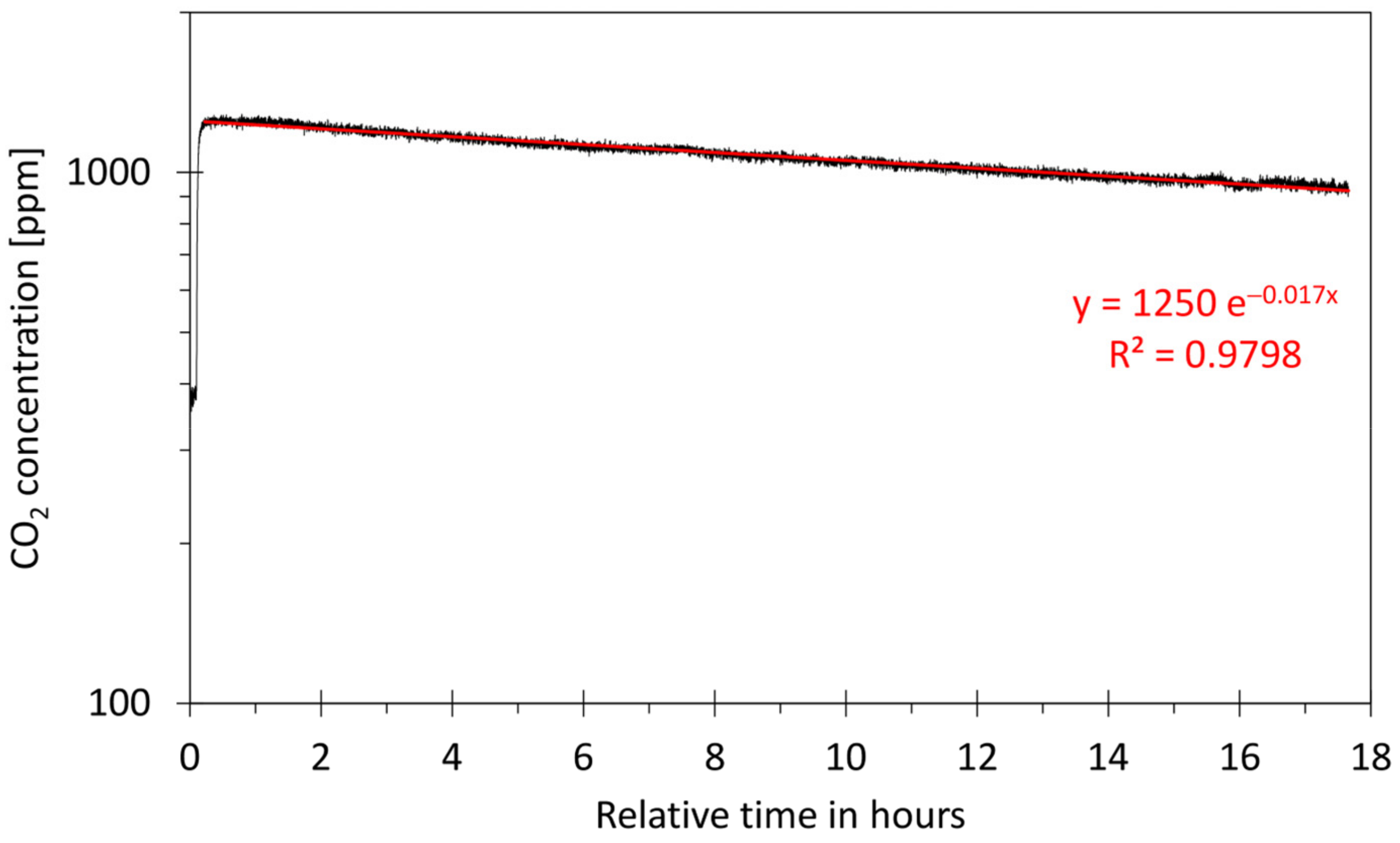
  • Airtightness of the calibration box: When the calibration box is not completely airtight, the calibration conditions will gradually degrade over time. To evaluate the importance of leakages, the tracer gas method was used. For this, the background concentration of CO2 in ambient air was measured first. Then, about 5 mL of CO2 was introduced into the calibration box using a syringe so that the CO2 concentration inside the box was substantially higher than outside the box. After some minutes, the sensor reached a stable value. The exponential decay of the tracer gas in the box was monitored for a period of about 20 h. The air exchange rate, which is expressed in air change per hour (h−1), was calculated with the formulas given in the Supplementary Material [77,78,79,80,81,82]. A calibration box that was sufficiently airtight throughout the calibration experiment (<5% of the total volume) is an indication that the method used was sufficiently valid;
  • Similarity with the factory-calibration: Some sensors, such as the ones measuring T, RH, or CO2, are often factory-calibrated. Although their calibration is often not well documented and unreliable [83], the measurements can be expected to have at least some similarity to the reference values. Therefore, the calibration curve is expected to be linear with an intercept and a slope around 0 and 1, respectively. A strong deviation from that expectation is an indication that something is wrong with the calibration (or with the sensor). This test is only valid for new sensors because they age over time and their calibration will change;
  • Similarity with the reference: For some calibration methods, the parameter to be measured is changed according to a predefined test program. A strong deviation of the sensor from the imposed test program is an indication that something is wrong;
  • Similarity between different sensors: If identical sensors or a set of factory-calibrated sensors are simultaneously calibrated, then minor differences between the calibration curves are expected;
  • Replicability of the calibration method: When a calibration method is applied on different sensors of the same type using different calibration boxes, different equipment, and different regions (i.e., what is the effect of the high RH in a tropical climate?), the calibration curves are expected to be similar. The occurrence of significant differences between the experiments indicate a lack of replicability;
  • Similarity with a golden standard: The calibration of the T/RH sensors was also performed by VITO, Belgium, using a closed stainless-steel exposure test chamber (Weiss Technik, Germany) with a total internal volume of the chamber at 1.0 m³. During the performed tests, the exposure test chamber was supplied with a constant and controlled flow of clean humidified air. The environmental conditions inside the chamber were constantly controlled and changed according to a test program to realize a consecutive series of T and RH levels. The homogeneity of the chamber’s inner atmosphere was provided by an active mixer installed next to the inlet of the chamber. The T and RH inside the exposure test chamber were continuously monitored and recorded using integrated and calibrated T/RH monitors mounted near the exhaust of the chamber. The reference monitoring devices are yearly calibrated by Weiss. During the development stage of low-cost calibration methods, it is useful to compare low-cost calibrations with reference calibrations that are considered as the golden standard. The more resemblances there are between both calibration curves, the more reliable the low-cost calibration method is.

2.7. Field Study

The air quality in Santa Clara, Cuba, had been already analyzed in previous studies [84]. That expertise was used to select the measuring locations summarized in Table 3. The field study consisted of a short measurement campaign at three different locations (Figure 5): (1) the Yabu site located northwest of the city in a rural region away from roads; (2) the farm site located in a rural area where the wind blows the air towards the city; and (3) the doctor’s office site in the center of the city where the air quality is affected by emissions from traffic and industry in the vicinity (e.g., production of pneumatic tires). The devices were placed at a height of 2.5 m above ground level, according to Cuban standard [85]. At the doctor’s office and at Yabu, the monitoring systems were hung in the window openings. The window openings were located at least 1 m from buildings, trees, and/or other obstructions. At the farm site, the monitoring system was hung underneath the porch. The calibration of the raw data obtained by the monitoring systems was performed as post-processing using Microsoft Excel. The two-step method had the advantage of allowing others to check the calibration of the collected data and roll back when an error was made in the calculations.

3. Results and Discussion

3.1. Airtightness of the Calibration Boxes

Before calibration experiments were carried out, it was necessary to check how airtight the calibration box was. The ambient CO2 concentration before the airtightness test was 376 ± 8 ppm. Then, the CO2 gas was injected. Once the CO2 concentration reached its maximum value (i.e., 1267 ppm), the experiment was started. During a period of 17.5 h, the CO2 concentration exponentially dropped to 935 ppm (see Figure 6). The calibration box had an air exchange rate of 0.02674 h−1. Since the calibration experiments lasted no more than 2 h, a loss of the entire air inside the box of about 5% could be considered as sufficiently small. It can be concluded that the plastic box was sufficiently airtight to use in calibration experiments.

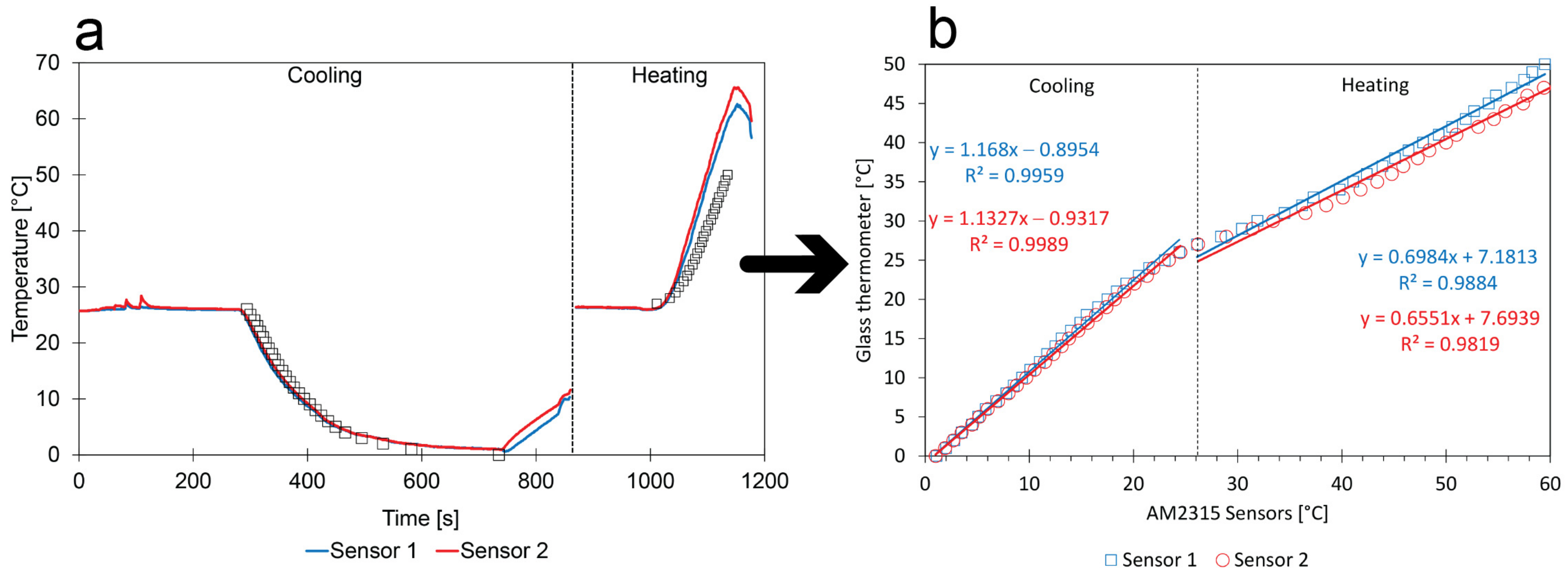
3.2. Temperature Calibration

Figure 7 shows the results of two different sensors simultaneously calibrated in the same box. The calibration consisted of a cooling and a heating process. The evolution of the T could not be imposed by a predefined test program, but was monitored with a glass thermometer (i.e., the reference measurement). The cooling process took about 17 min. The heating process was determined by the T set by the thermostat, which was 65 °C. The T raised from room T to the set T in about 5 min. The reference values in Figure 7b are shown in the vertical axis so that regression functions directly give the correct formula to convert measured values into the corrected ones. The following observations could be made:
  • Calibration method: The uncontrolled test program could be monitored with a glass thermometer. The calibration curve was obtained by plotting the sensor measurements with the corresponding glass thermometer measurements observed at the same moment;
  • Low impact of random errors: The scattering of the calibration points around the linear regressions is small, suggesting that the method resulted in small random errors;
  • Comparison between sensors: There is a good similarity between the calibration curves of the two different sensors. Even when the calibration contains a constant error, it is still possible to compensate for calibration differences between sensors;
  • Comparison with factory-calibration: In the early stage of the lifetime of factory-calibrated sensors, the low-cost calibration and factory-calibration should match. For the cooling process, this was indeed the case, but not for the heating process;
  • Comparison with the reference: During the heating process, there is no close similarity between sensor and glass thermometer measurements (see Figure 7a). In principle, a polynomial regression with order 3 can be used to describe the entire set of calibration points in Figure 7b covering the total range of 0–63 °C (i.e., correlation coefficient: 0.9979 and 0.9987 for sensors 1 and 2, respectively). However, the indicators used to evaluate the calibration methods suggest that the reliability of the heating process must be checked more closely.
A similar calibration experiment was performed with a golden standard. Figure 8a shows how the T changed over time according to a predefined program. For every transition between consecutive plateaus (see moments between the black rectangles in Figure 8a), some time was needed before the T reached a stable value. The following observations could be made:
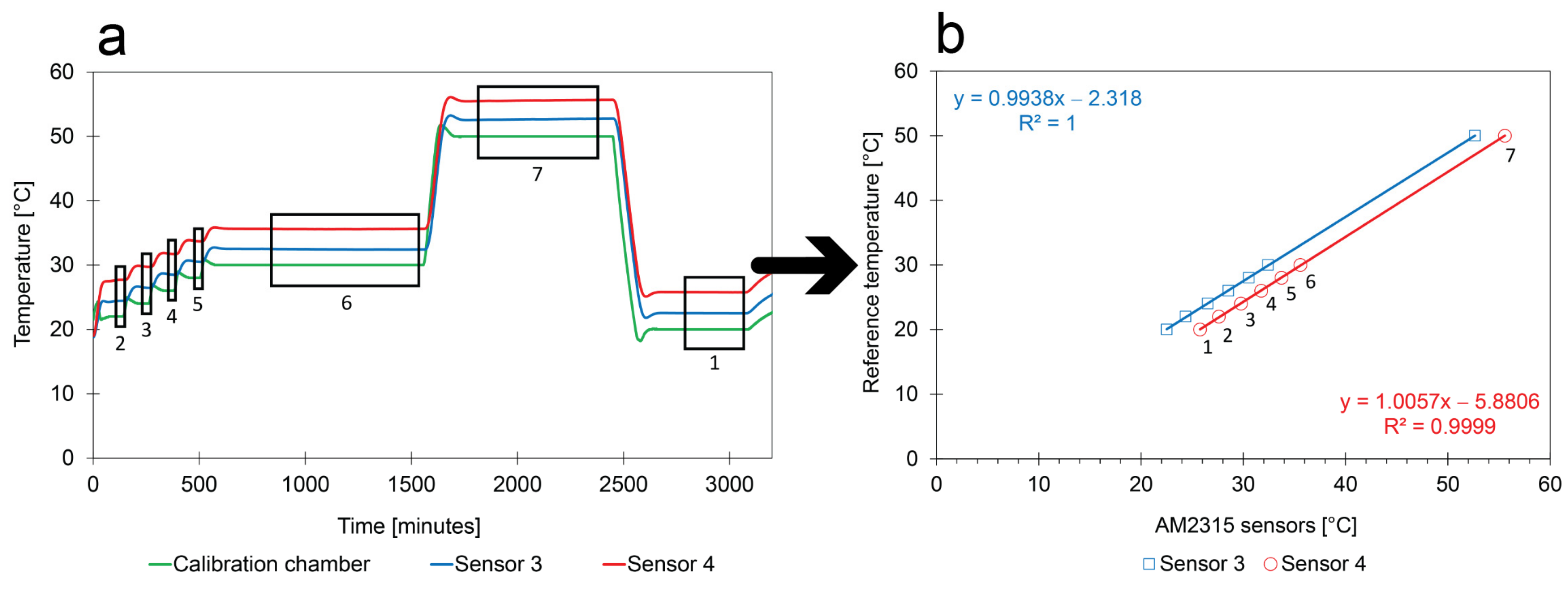
  • Calibration method: Only a limited number of periods have a stable but known T. These periods are numbered in Figure 8. The average temperatures were calculated for the second half of the plateaus because the chamber and the sensors needed some time to reach equilibrium;
  • Comparison between sensors and with reference: The behavior of the sensors and the test program as measured by the reference instrument show similar trends over time. In addition, there is a similarity between the calibration curves of the two different sensors (i.e., a linear trend, a slope of around 1). However, the intercepts are clearly different from 0, suggesting that the quality of pre-calibrated sensors needs to be improved before they can be used in the field tests. In addition, it shows that the calibration during the heating process shown in Figure 7 is incorrect. The other indicators appear to be sensitive enough to identify the calibration error.
The T calibration experiment using the heating process was repeated at a lower heating rate. In this experiment, the lid did not entirely close the box to allow better dissipation of the heat. In addition, the fan was stopped if the set point was reached. The moment that the T started to drop, the next set point was introduced in the thermostat and the fan was switched on again. As a result, there was first a small drop followed by an increase in T. There was no full control of the staircase function, but the increase in T appeared to be sufficiently slow to obtain a calibration that was similar to the ones obtained with the golden standard.
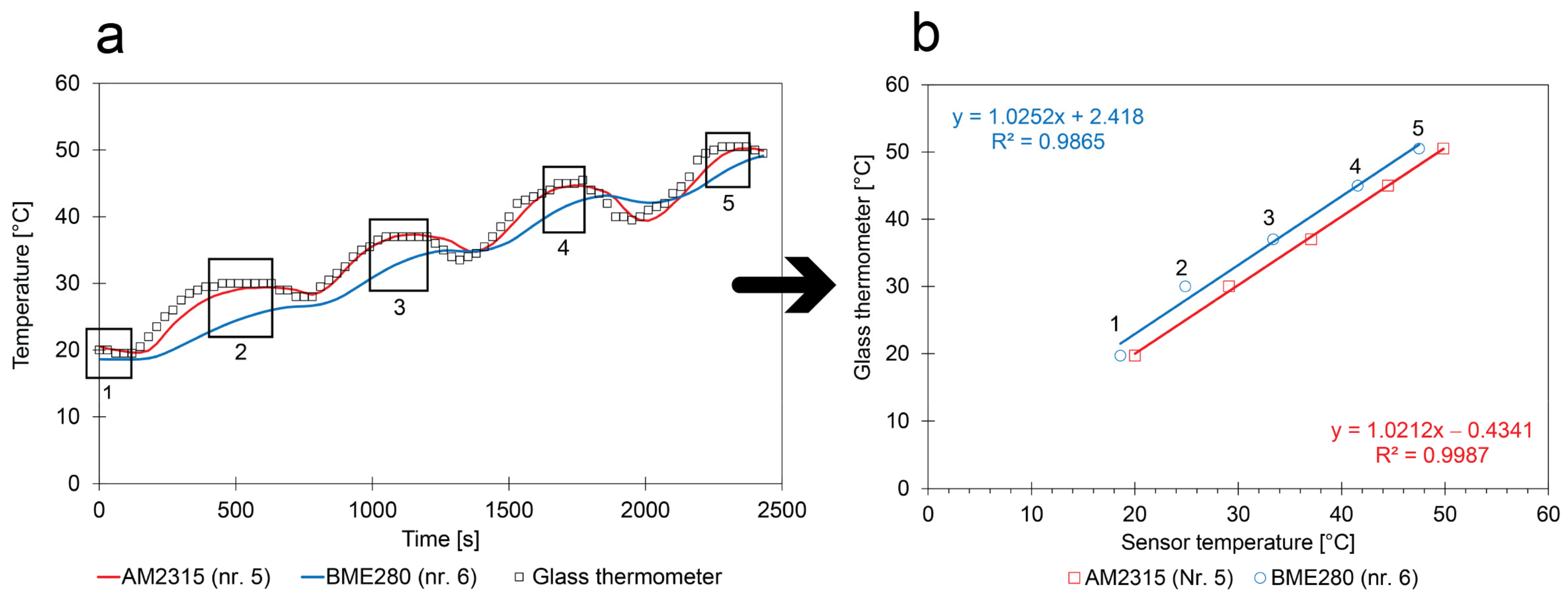
  • Absolute calibration method: The calibration relies on the calculation of the average T within the short periods where the T is stable. These periods are numbered in Figure 9. The average temperatures are compared with the glass thermometer measurements;
  • Relative calibration method: When sensors experience the same conditions during the same calibration experiment, differences between them can be compensated. This compensation is even possible when the low-cost calibration method is unable to accurately determine the absolute values. Consequently, differences in trends from two monitoring campaigns performed in parallel during the field study can be studied in a reliable way;
  • Comparison with the reference: The experiments suggest that the behavior of the sensors in comparison with the reference show several small differences. The AM2315 follows the values obtained with the glass thermometer with some delay (see Figure 9a). The BME280 sensor appears to be less sensitive to the changes in the calibration box;
  • Comparison between sensors: The slopes of the calibration curves of the two factory-calibrated sensors were close to 1 and the intercepts had a small deviation from 0. The calibration curves also showed more similarities with the ones obtained with cooling (see Figure 7). This indicates that cooling or heating rates should be sufficiently small to obtain a correct calibration;
  • Replicability of the calibration method: The same calibration method was used to calibrate a set of low-cost sensors in different regions (Figure 7 in Cuba; Figure 9 in Belgium) using different calibration boxes and with different equipment. Except for the heating process shown in Figure 7, they all gave a linear regression with similarities to the factory calibration. No obvious differences between the low-cost calibration and the golden standard (Figure 8 performed in Belgium) could be observed. This means that the calibration method resulted in reproducible results and that factory calibrations can be improved.

3.3. Relative Humidity Calibration

Figure 10 shows the behavior of two identical AM2315 sensors (the same sensors as in Figure 7) during the RH calibration. To obtain a calibration curve that corrects the RH readings measured by the sensors, a scatter plot was made between the theoretical RH that was determined from the density of the glycerol solution and the sensor measurement after the box reached equilibrium. Each calibration point in Figure 10b is a different experiment that required time before a constant RH was obtained. The different calibration experiments were concatenated into a single time series (see Figure 10a). The trend of series 1 in Figure 10a using the pure glycerol solution was truncated because it took about 14 h to perform that experiment.
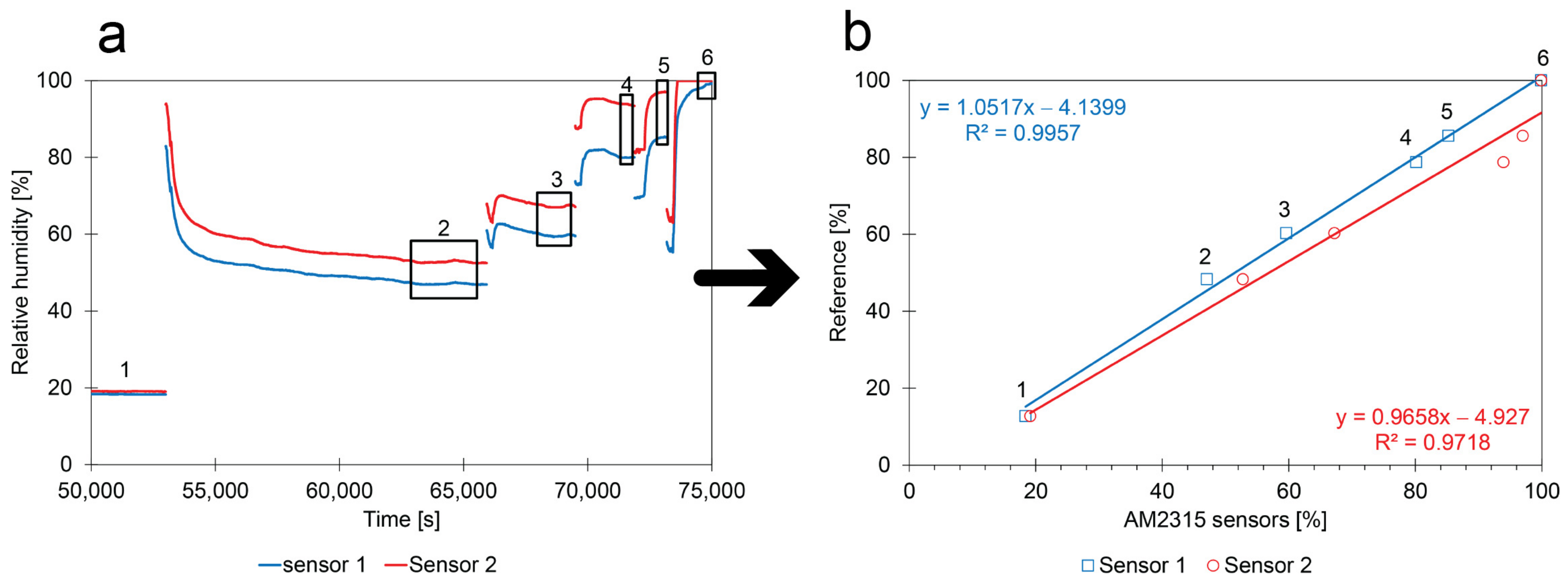
  • Calibration method: The calibration experiments in Figure 10a were stopped once the RH reached a stable value. The average value was calculated from the stable periods shown in the numbered boxes and compared with the theoretical values that were obtained with the glycerol solution. The results show that the calibration performed by the manufacturer can be improved with low-cost calibration experiments (at least in a relative way);
  • Low random error: The calibration points follow a linear trend, suggesting that the contribution of random errors is low;
  • Comparison between sensors: The linear calibration functions of both sensors show similarities. The slopes of the calibration curves are close to 1 as expected. The intercepts are similar, but deviate from zero.
The calibration experiment performed with a golden standard was also used to evaluate the RH measurements of the same AM2315 sensors as the ones used in Figure 8. Figure 11a shows how the RH changed over time according to a predefined program. Calibration points 1 to 4 were determined at a T of 50 °C to reach the lower values. For points 5 to 9, the constant T is representative for tropical weather.
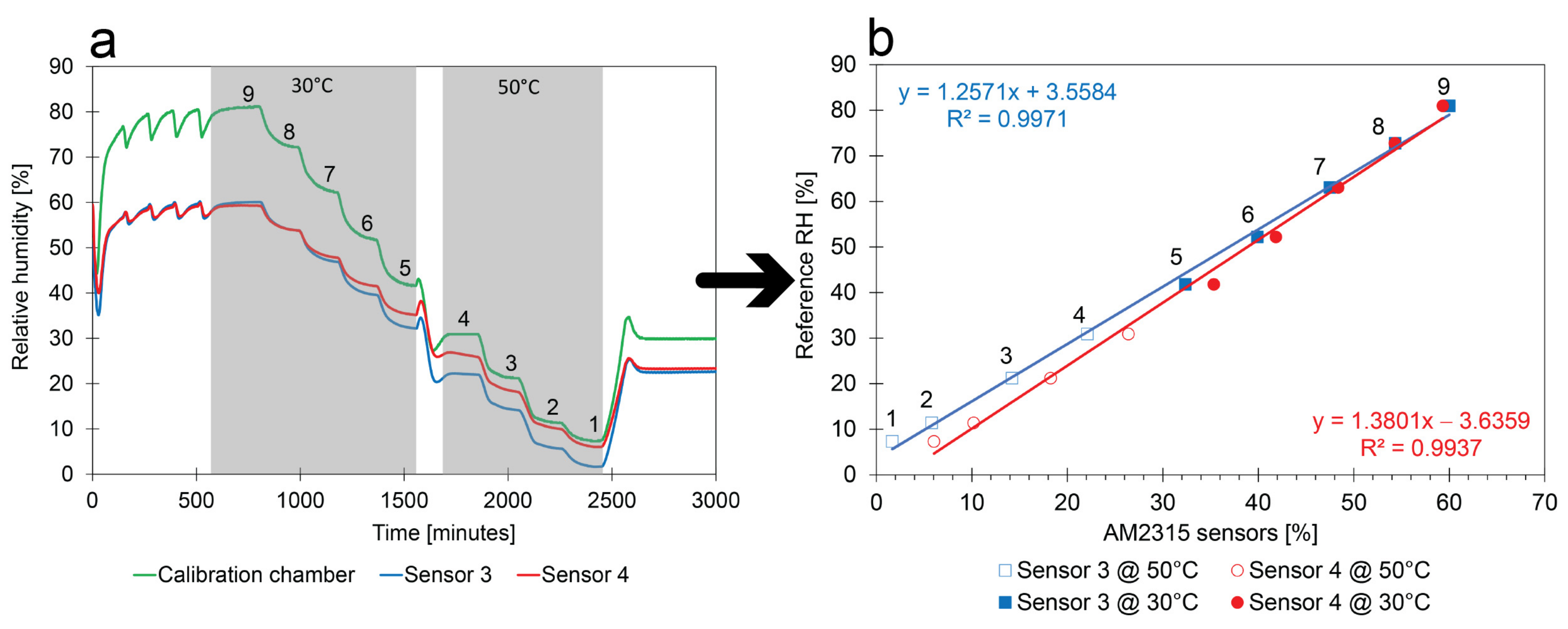
  • Calibration method:Figure 11b shows the linear calibration of the sensors. The calibration points show the relation between the average values of the numbered plateaus in Figure 11a and the corresponding RH measured by the climate chamber. Only the second half of the plateaus were considered because they were more stable;
  • Comparison between sensors: The slope and intercept of both sensors are similar but different enough to require additional calibration before they can be used in field measurements. In addition, the slope and intercept are close to the ones determined with the low-cost calibration methods. It should be remarked that the set of calibration points determined at 30 °C and the set of 50 °C do not entirely match the linear regression. There is a small impact of the T on the RH measurements;
  • Replicability of the calibration method: The calibration method has been tested on several sensors of the same type. The same calibration box and equipment have been used to independently perform the six experiments of Figure 10a. Calibration is also performed with a golden standard. No obvious differences could be observed between the linear regressions. The similarities show that the low-cost RH calibration is sufficiently reliable and that factory calibrations of the sensors can be improved.

3.4. CO2 Calibration

The behavior of two identical COZIR-A CO2 sensors enduring the same calibration process is shown in Figure 12a. Once the box was closed, the sensors measured the natural background concentration of CO2 in ambient air. When the air was pumped through the Ca(OH)2/NaOH solution, the CO2 concentration decreased below the detection limit of the sensors (i.e., nearly zero). Then, the CO2 gas in the syringe was introduced in three consecutive steps. At every CO2 injection, the sensor signal suddenly increased. The sensor readout followed the jumps of a staircase function, while the room T and RH inside the box remained constant (i.e., 27 °C and 65%).
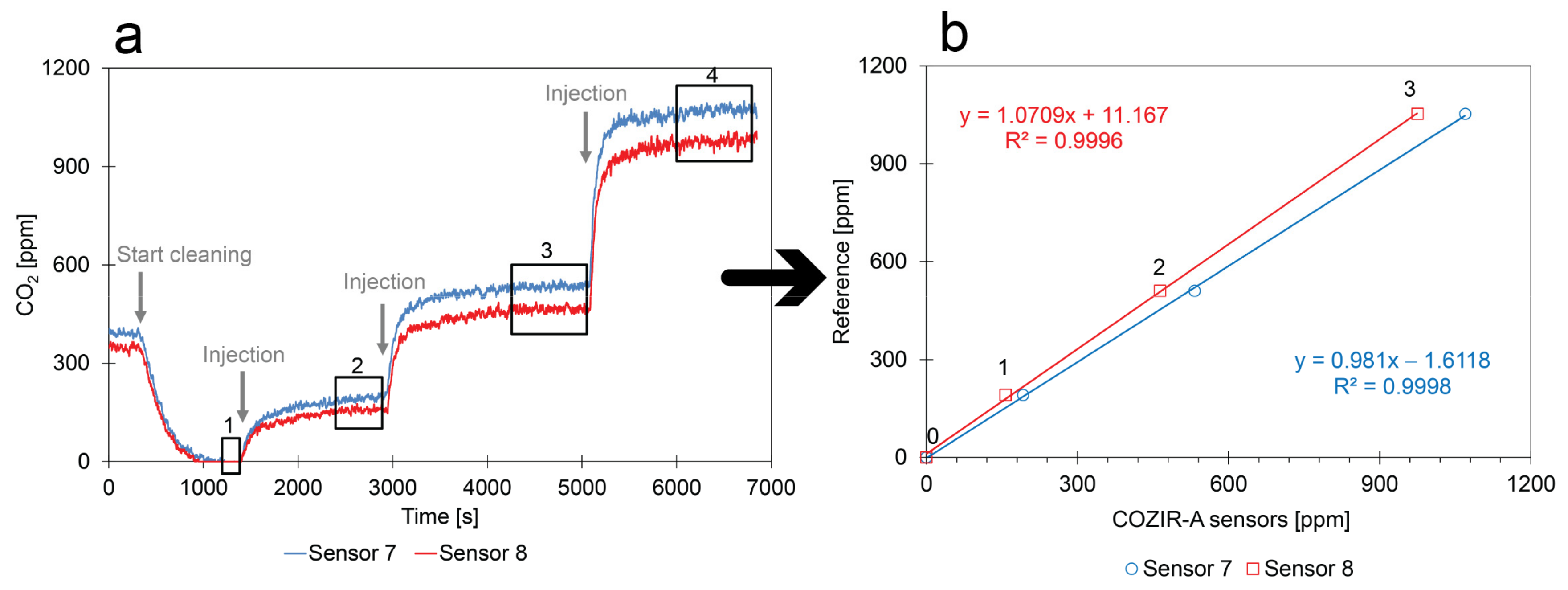
  • Calibration method: Because all CO2 inside the closed box was removed and because known amounts of CO2 were injected into the box, the staircase function was fully controlled. However, only the concentrations of the plateaus could be calculated from the injected amounts and used for calibration. Consequently, the average values of the numbered rectangles in Figure 12a were used for calibration;
  • Limited random errors: The mathematical relation of the calibration points can be described by linear regression (see Figure 12b). This suggests that the contribution of random errors during the experiment is low;
  • Comparison between sensors: Figure 12a shows that both sensors follow the same trend, but that they respond slightly differently to the same environment.
A similar calibration experiment as in Figure 12 was performed without the cleaning of the air. This means that known amounts of CO2 were introduced inside the closed box that contained air with an unknown amount of CO2. However, it is known that the background concentration in ambient air is around 412 ppm. The calibration was performed by the standard addition method.
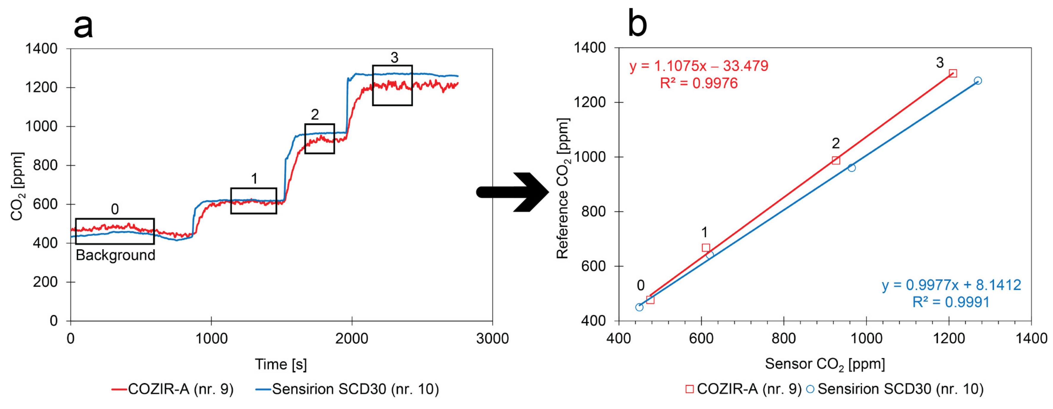
  • Calibration method: The two factory-calibrated sensors measured a different background concentration (rectangle 0 in Figure 13a) in the closed box (COZIR-A: 476 ppm; Sensirion SCD30: 450 ppm). From the measured background concentrations and the calculated concentrations that were introduced, the reference concentrations of rectangles 1, 2, and 3 could be determined;
  • Comparison between sensors: Although the intercept of the calibration curves might contain a small but constant error due to an error in the measurement of the background concentration, the slopes can be accurately determined;
  • Replicability of the calibration method: Different kinds of factory-calibrated sensors have been tested with two different calibration methods. The linear regressions given in Figure 12 and Figure 13 show sufficient similarities to conclude that the low-cost CO2 calibration methods are sufficiently reliable and that the factory calibration of the sensors can be improved.

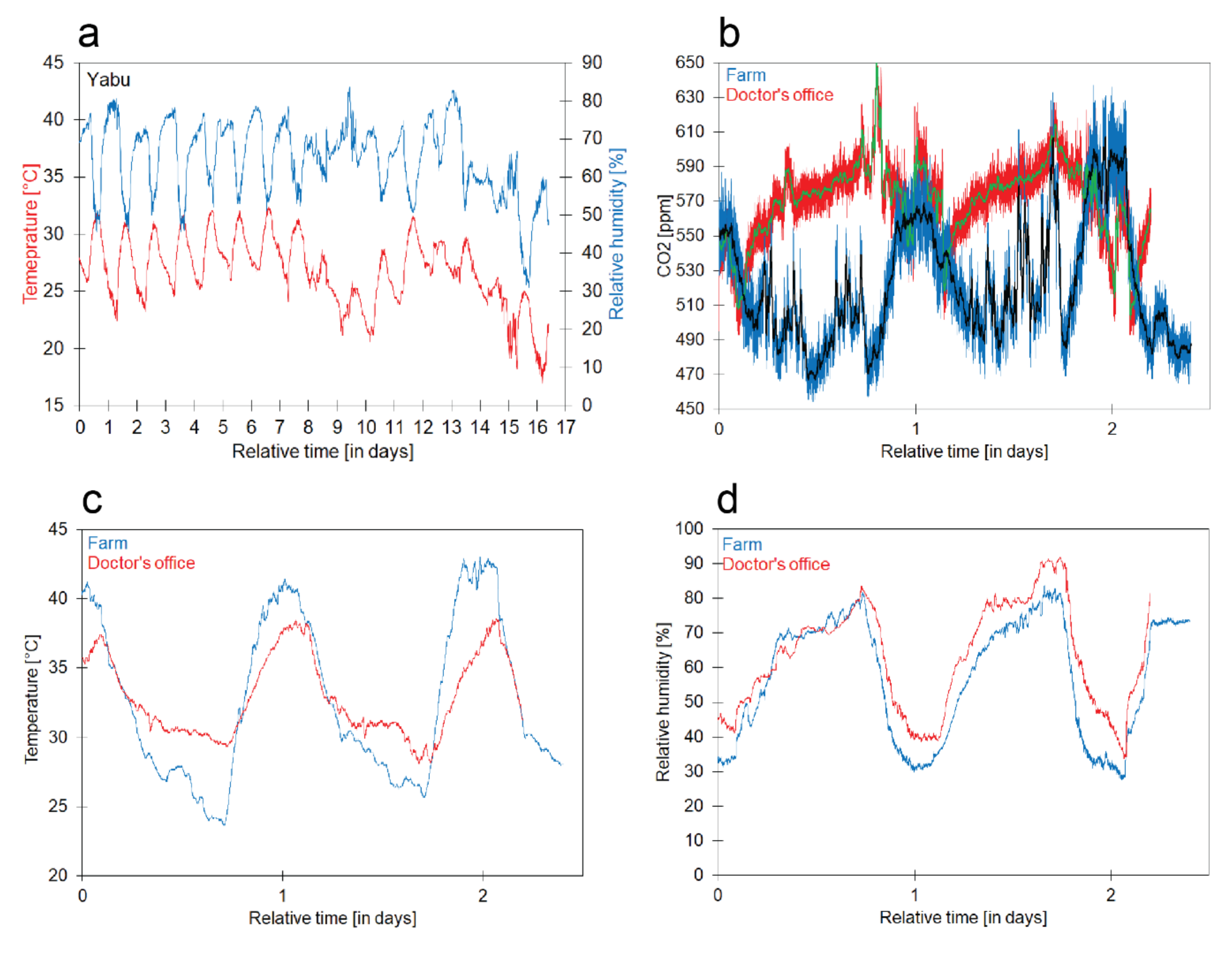
3.5. Results of the Field Study

Table 4 presents the descriptive statistics of the time series recorded during the field study. The standard deviations from the two sites measured in parallel, the farm and doctor’s office, show that environmental parameters fluctuate more at the farm. In addition, the time series of the three parameters show different signs in the asymmetry coefficients. The values of the coefficient indicate that the distribution of the data around their average is not symmetric (i.e., the positive value means that the right tail is longer; the negative value means a skewness to the left). The statistical overview of Table 4 gives a good overview of the three sites and makes comparison easy, but a substantial amount of information that is present in the dynamics of temporal trends is lost in the descriptive statistics. Therefore, measurement campaigns with reliable low-cost monitoring systems are an important added value. Unfortunately, this way of working was hampered by regular power cuts in the city. In addition, additional efforts are needed in data post-processing to suppress noise and remove spikes. For example, the CO2 measurements at the farm contained several spikes, with a value of 0 or 2 ppm. They were removed by a simple filter: if the concentration was below 100 ppm, then the data point was replaced by the average value of the previous and next data point.
Figure 14a shows the calibrated results of T and RH during the field experiment at the Yabu site. During that period, there was no precipitation. In this measuring campaign, the trends clearly showed day-night cycles where T and RH were in an opposite phase. For each day, between 5:30 and 7:00, the T dropped down to a minimum of 21–25 °C, while the RH reached a maximum of 80–87%. Around 13:00 and 15:00, the T reached a maximum of 26–28 °C, while the RH during that period was 53–70%. The period of the day-night cycles varied around 24 h but, due to small random changes of the minima and the maxima in the given periods, the cyclic pattern was quasi-periodic. In addition, the local maxima and minima varied. This short measurement campaign suggests that in-house built monitoring systems can be used to generate useful information that is complementary to the statistical data.
Figure 14b–d shows the results of CO2, T, and RH measured in parallel at the farm and the doctor’s office during the field tests during 4–6 March 2020. The calibration of both sensors ensures that the differences between locations are only caused by the location and not by measuring errors. At both locations, T, RH, and CO2 show diurnal cycles. For the farm, the minima and maxima of the T are somewhat more extreme. The RH at both locations shows a similar trend, but the minima observed at the farm are somewhat lower. This suggests that, at the farm, the nights are cooler and less humid. The CO2 trend at the farm shows similar dynamics to the T, with maxima at around midnight. The CO2 trend at the doctor’s office is more complex. What is striking is the noise in Figure 14b. The noise was suppressed by using a centered moving window with a window size of 10 min. The comparison demonstrates that calibrated low-cost monitoring systems can generate valuable information from which conclusions can be drawn.
Calibration procedures and field tests allowed for reaching the maximum performance reflected in the datasheets of the sensors. Therefore, the system is considered suitable as a measurement instrument, as long as a resolution greater than 0.1 °C for T, 2% for RH, and 30 ppm for CO2 is not required. Furthermore, when the maximum values exceed 80 °C or 2000 ppm of CO2, they will cause saturation of the outputs. It is important to mention that the maximum operating temperature for Arduino Mega 2560 computing unit is 85 °C; thus, it is not recommended to exceed this value. The system is not suitable for obtaining measurement resolutions higher than those mentioned or more extreme operating conditions.

4. Conclusions

There is abundant information available to build low-cost monitoring systems that can measure parameters such as temperature, relative humidity, and CO2. However, applications using such devices rely on the calibration of the manufacturer. This means that the accuracy of such devices is unclear. Some studies compare low-cost monitoring systems with high-end reference instruments. Unfortunately, not everyone has access to such instruments. This contribution proposes low-cost calibration methods for temperature, relative humidity, and CO2 that can be performed in a laboratory situated in a tropical climate. The calibration methods were used for several sensors using different calibration boxes, equipment, and regions where the laboratory is located. All situations resulted in similar calibration results. The air exchange rates suggested that the airtightness of the calibration box was sufficient. In addition, the calibrations for temperature and relative humidity obtained with the low-cost calibration methods were in line with the golden standard. The experiments showed that factory calibrations can be improved and differences between sensors can be compensated. The field campaigns demonstrated that the calibrated low-cost monitoring systems could be used as a low-cost scientific instrument. The quality of the data generated by that scientific instrument was perhaps not as good as that of state-of-the-art reference instruments, but the field test showed that it was good enough to draw conclusions from the measurement campaigns and that the dynamics in trends gave valuable information that was complementary to a statistical analysis of larger periods. By using the mindset of a satisficer, numerous institutions and researchers from low- and mid-income countries gain access to research infrastructure to solve local problems in a reliable way. This makes scientific research more inclusive. Moreover, technology is systematically improving, so data quality generated by low-cost scientific instruments will increase over time. The satisficer method will become more performant over time.

Supplementary Materials

The following supporting information can be downloaded at: https://www.mdpi.com/article/10.3390/atmos14020191/s1, Figure S1. Schematic overview illustrating the pressure difference between the atmosphere and syringe.; Table S1. Overview of the symbols used in the equations.; Equation (S1)–(S7).

Author Contributions

R.A.G.R.: Processing of results obtained in the air exchange rate determination, calibration of the CO2 sensors, and manuscript preparation. L.E.M.H.: Processing of results obtained in the calibration of the temperature and relative humidity sensors, manuscript preparation. O.S.: Research conception and design, review and approval of the final version of the manuscript. E.H.R.: Design of the low-cost monitoring system. D.A.S.: Research conception and design, review and approval of the final version of the manuscript. M.C.M.P.: Sampling site selection strategy. Data processing and analysis obtained in the field study. V.N.C.: Sampling site selection strategy. Data processing and analysis obtained in the field study. W.J.: Research conception and design, review and approval of the final version of the manuscript. A.M.L.: Assembly of the low-cost monitoring system, review and approval of the final version of the manuscript. All authors have read and agreed to the published version of the manuscript.

Funding

The present work has been supported by the VLIR-UOS Program as a South Initiative Project SI-2019 nr. CU2019SIN242B124 “AIR@PORT: Low-cost decision support system to evaluate the impact of ships on the air quality in the port city Cienfuegos”. Additional financial support has been given by the common Global Minds project BE2017GMHVLHC106 of all Flemish Universities of Applied Sciences and Arts.

Institutional Review Board Statement

Not applicable.

Informed Consent Statement

Not applicable.

Data Availability Statement

All data used in this study are available upon request.

Acknowledgments

The authors thank VLIR-UOS for their financial support of the South Initiative Project SI-2019 nr. CU2019SIN242B124 “AIR@PORT: Low-cost decision support system to evaluate the impact of ships on the air quality in the port city Cienfuegos”. They are also grateful for the additional support by the Global Minds project BE2017GMHVLHC106.

Conflicts of Interest

The authors declare no conflict of interest.

References

  1. Mannucci, P.; Franchini, M. Health Effects of Ambient Air Pollution in Developing Countries. IJERPH 2017, 14, 1048. [Google Scholar] [CrossRef] [PubMed]
  2. Chen, B.H.; Hong, C.L.; Pandey, M.R.; Smith, K.R. Indoor Air Pollution in Developing Countries. World Health Stat. Q. 1990, 43, 127–137. [Google Scholar] [PubMed]
  3. Pinder, R.W.; Klopp, J.M.; Kleiman, G.; Hagler, G.S.W.; Awe, Y.; Terry, S. Opportunities and Challenges for Filling the Air Quality Data Gap in Low- and Middle-Income Countries. Atmos. Environ. 2019, 215, 116794. [Google Scholar] [CrossRef] [PubMed]
  4. Ibrahim, M.F.; Hod, R.; Nawi, A.M.; Sahani, M. Association between Ambient Air Pollution and Childhood Respiratory Diseases in Low- and Middle-Income Asian Countries: A Systematic Review. Atmos. Environ. 2021, 256, 118422. [Google Scholar] [CrossRef]
  5. Helmut, M. Air Pollution in Cities. Atmos. Environ. 1999, 33, 4029–4037. [Google Scholar]
  6. Hodoli, C.G.; Coulon, F.; Mead, M.I. Source Identification with High-Temporal Resolution Data from Low-Cost Sensors Using Bivariate Polar Plots in Urban Areas of Ghana. Environ. Pollut. 2023, 317, 120448. [Google Scholar] [CrossRef]
  7. deSouza, P.; Nthusi, V.; Klopp, J.; Shaw, B.; Ho, W.; Saffell, J.; Jones, R.; Ratti, C. A Nairobi Experiment in Using Low Cost Air Quality Monitors. Clean Air J. 2017, 27, 12–42. [Google Scholar] [CrossRef]
  8. Abraham, S.; Li, X. A Cost-Effective Wireless Sensor Network System for Indoor Air Quality Monitoring Applications. Procedia Comput. Sci. 2014, 34, 165–171. [Google Scholar] [CrossRef] [Green Version]
  9. Aguiar, E.F.K.; Roig, H.L.; Mancini, L.H.; de Carvalho, E.N.C.B. Low-Cost Sensors Calibration for Monitoring Air Quality in the Federal District—Brazil. JEP 2015, 6, 173–189. [Google Scholar] [CrossRef] [Green Version]
  10. Zimmerman, N.; Presto, A.A.; Kumar, S.P.N.; Gu, J.; Hauryliuk, A.; Robinson, E.S.; Robinson, A.L.; Subramanian, R. A Machine Learning Calibration Model Using Random Forests to Improve Sensor Performance for Lower-Cost Air Quality Monitoring. Atmos. Meas. Tech. 2018, 11, 291–313. [Google Scholar] [CrossRef] [Green Version]
  11. Morawska, L.; Thai, P.K.; Liu, X.; Asumadu-Sakyi, A.; Ayoko, G.; Bartonova, A.; Bedini, A.; Chai, F.; Christensen, B.; Dunbabin, M.; et al. Applications of Low-Cost Sensing Technologies for Air Quality Monitoring and Exposure Assessment: How Far Have They Gone? Environ. Int. 2018, 116, 286–299. [Google Scholar] [CrossRef]
  12. Schalm, O.; Cabal, A.; Anaf, W.; Leyva Pernia, D.; Callier, J.; Ortega, N. A Decision Support System for Preventive Conservation: From Measurements towards Decision Making. Eur. Phys. J. Plus 2019, 134, 74. [Google Scholar] [CrossRef]
  13. Anaf, W.; Leyva Pernia, D.; Schalm, O. Standardized Indoor Air Quality Assessments as a Tool to Prepare Heritage Guardians for Changing Preservation Conditions Due to Climate Change. Geosci. J. 2018, 8, 276. [Google Scholar] [CrossRef] [Green Version]
  14. Gaudenzi Asinelli, M.; Serra Serra, M.; Molera Marimòn, J.; Serra Espaulella, J. The SmARTS_Museum_V1: An Open Hardware Device for Remote Monitoring of Cultural Heritage Indoor Environments. HardwareX 2018, 4, e00028. [Google Scholar] [CrossRef]
  15. CEN EN 15757:2010. Conservation of Cultural Property: Specifications for Temperature and Relative Humidity to Limit Climate-Induced Mechanical Damage in Organic Hygroscopic Materials. European Committee for Standardization (CEN): Brussels, Belgium, 2010.
  16. Silva, H.E.; Coelho, G.B.A.; Henriques, F.M.A. Climate Monitoring in World Heritage List Buildings with Low-Cost Data Loggers: The Case of the Jerónimos Monastery in Lisbon. JOBE 2020, 28, 101029. [Google Scholar] [CrossRef]
  17. Tarasick, D.W.; Smit, H.G.J.; Thompson, A.M.; Morris, G.A.; Witte, J.C.; Davies, J.; Nakano, T.; Van Malderen, R.; Stauffer, R.M.; Johnson, B.J.; et al. Improving ECC Ozonesonde Data Quality: Assessment of Current Methods and Outstanding Issues. Earth Space Sci 2021, 8, e2019EA000914. [Google Scholar] [CrossRef]
  18. Van Malderen, R.; De Muer, D.; De Backer, H.; Poyraz, D.; Verstraeten, W.W.; De Bock, V.; Delcloo, A.W.; Mangold, A.; Laffineur, Q.; Allaart, M.; et al. Fifty Years of Balloon-Borne Ozone Profile Measurements at Uccle, Belgium: A Short History, the Scientific Relevance, and the Achievements in Understanding the Vertical Ozone Distribution. Atmos. Chem. Phys. 2021, 21, 12385–12411. [Google Scholar] [CrossRef]
  19. Rodriguez-Vasquez, K.A.; Cole, A.M.; Yordanova, D.; Smith, R.; Kidwell, N.M. AIRduino: On-Demand Atmospheric Secondary Organic Aerosol Measurements with a Mobile Arduino Multisensor. J. Chem. Educ. 2020, 97, 838–844. [Google Scholar] [CrossRef]
  20. Mijling, B.; Jiang, Q.; de Jonge, D.; Bocconi, S. Field Calibration of Electrochemical NO2 Sensors in a Citizen Science Context. Atmos. Meas. Tech. 2018, 11, 1297–1312. [Google Scholar] [CrossRef] [Green Version]
  21. Watne, Å.K.; Linden, J.; Willhelmsson, J.; Fridén, H.; Gustafsson, M.; Castell, N. Tackling Data Quality When Using Low-Cost Air Quality Sensors in Citizen Science Projects. Front. Environ. Sci. 2021, 9, 733634. [Google Scholar] [CrossRef]
  22. Wallace, L.; Bi, J.; Ott, W.R.; Sarnat, J.; Liu, Y. Calibration of Low-Cost PurpleAir Outdoor Monitors Using an Improved Method of Calculating PM. Atmos. Environ. 2021, 256, 118432. [Google Scholar] [CrossRef]
  23. Karaoghlanian, N.; Noureddine, B.; Saliba, N.; Shihadeh, A.; Lakkis, I. Low Cost Air Quality Sensors “PurpleAir” Calibration and Inter-Calibration Dataset in the Context of Beirut, Lebanon. Data Br. 2022, 41, 108008. [Google Scholar] [CrossRef] [PubMed]
  24. Karagulian, F.; Barbiere, M.; Kotsev, A.; Spinelle, L.; Gerboles, M.; Lagler, F.; Redon, N.; Crunaire, S.; Borowiak, A. Review of the Performance of Low-Cost Sensors for Air Quality Monitoring. Atmosphere 2019, 10, 506. [Google Scholar] [CrossRef] [Green Version]
  25. Narayana, M.V.; Jalihal, D.; Nagendra, S.M.S. Establishing A Sustainable Low-Cost Air Quality Monitoring Setup: A Survey of the State-of-the-Art. Sensors 2022, 22, 394. [Google Scholar] [CrossRef] [PubMed]
  26. Singh, D.; Dahiya, M.; Kumar, R.; Nanda, C. Sensors and Systems for Air Quality Assessment Monitoring and Management: A Review. J. Environ. Manag. 2021, 289, 112510. [Google Scholar] [CrossRef] [PubMed]
  27. Chojer, H.; Branco, P.T.B.S.; Martins, F.G.; Alvim-Ferraz, M.C.M.; Sousa, S.I.V. Development of Low-Cost Indoor Air Quality Monitoring Devices: Recent Advancements. Sci. Total Environ. 2020, 727, 138385. [Google Scholar] [CrossRef] [PubMed]
  28. Bigi, A.; Mueller, M.; Grange, S.K.; Ghermandi, G.; Hueglin, C. Performance of NO, NO2 Low Cost Sensors and Three Calibration Approaches within a Real World Application. Atmos. Meas. Tech. 2018, 11, 3717–3735. [Google Scholar] [CrossRef] [Green Version]
  29. Bean, J.K. Evaluation Methods for Low-Cost Particulate Matter Sensors. Atmos. Meas. Tech. 2021, 14, 7369–7379. [Google Scholar] [CrossRef]
  30. Concas, F.; Mineraud, J.; Lagerspetz, E.; Varjonen, S.; Liu, X.; Puolamäki, K.; Nurmi, P.; Tarkoma, S. Low-Cost Outdoor Air Quality Monitoring and Sensor Calibration: A Survey and Critical Analysis. ACM Trans. Sens. Netw. (TOSN) 2021, 17, 1–44. [Google Scholar] [CrossRef]
  31. Venkatraman Jagatha, J.; Klausnitzer, A.; Chacón-Mateos, M.; Laquai, B.; Nieuwkoop, E.; van der Mark, P.; Vogt, U.; Schneider, C. Calibration Method for Particulate Matter Low-Cost Sensors Used in Ambient Air Quality Monitoring and Research. Sensors 2021, 21, 3960. [Google Scholar] [CrossRef]
  32. Artinano, B.; Narros, A.; Diaz, E.; Gomez, F.J.; Borge, R. Low-Cost Sensors for Urban Air Quality Monitoring: Preliminary Laboratory and in-Field Tests within the TECNAIRE-CM Project. In Proceedings of the 2019 5th Experiment International Conference (exp.at’19), Funchal, Portugal, 12–14 June 2019; pp. 462–466. [Google Scholar]
  33. Schalm, O.; Carro, G.; Lazarov, B.; Jacobs, W.; Stranger, M. Reliability of Lower-Cost Sensors in the Analysis of Indoor Air Quality on Board Ships. Atmosphere 2022, 13, 1579. [Google Scholar] [CrossRef]
  34. Mao, K.; Xu, J.; Jin, R.; Wang, Y.; Fang, K. A Fast Calibration Algorithm for Non-Dispersive Infrared Single Channel Carbon Dioxide Sensor Based on Deep Learning. Comput. Commun. 2021, 179, 175–182. [Google Scholar] [CrossRef]
  35. Schwartz, B. The Paradox of Choice: Why More Is Less; Harper Perennial: New York, NY, USA, 2005. [Google Scholar]
  36. Villanueva, F.; Ródenas, M.; Ruus, A.; Saffell, J.; Gabriel, M.F. Sampling and Analysis Techniques for Inorganic Air Pollutants in Indoor Air. Appl. Spectrosc. Rev. 2022, 57, 531–579. [Google Scholar] [CrossRef]
  37. Samad, A.; Obando Nuñez, D.R.; Solis Castillo, G.C.; Laquai, B.; Vogt, U. Effect of Relative Humidity and Air Temperature on the Results Obtained from Low-Cost Gas Sensors for Ambient Air Quality Measurements. Sensors 2020, 20, 5175. [Google Scholar] [CrossRef]
  38. Wei, P.; Ning, Z.; Ye, S.; Sun, L.; Yang, F.; Wong, K.; Westerdahl, D.; Louie, P. Impact Analysis of Temperature and Humidity Conditions on Electrochemical Sensor Response in Ambient Air Quality Monitoring. Sensors 2018, 18, 59. [Google Scholar] [CrossRef] [Green Version]
  39. Wahlborg, D.; Björling, M.; Mattsson, M. Evaluation of Field Calibration Methods and Performance of AQMesh, a Low-Cost Air Quality Monitor. Environ. Monit. Assess. 2021, 193, 251. [Google Scholar] [CrossRef]
  40. Gonzalez, A.; Boies, A.; Swason, J.; Kittelson, D. Field Calibration of Low-Cost Air Pollution Sensors. Atmos. Meas. Tech. Discuss. 2019, 12, 1–17. [Google Scholar] [CrossRef]
  41. Borrego, C.; Costa, A.M.; Ginja, J.; Amorim, M.; Coutinho, M.; Karatzas, K.; Sioumis, T.; Katsifarakis, N.; Konstantinidis, K.; De Vito, S.; et al. Assessment of Air Quality Microsensors versus Reference Methods: The EuNetAir Joint Exercise. Atmos. Environ. 2016, 147, 246–263. [Google Scholar] [CrossRef] [Green Version]
  42. Drewnick, F.; Böttger, T.; von der Weiden-Reinmüller, S.-L.; Zorn, S.R.; Klimach, T.; Schneider, J.; Borrmann, S. Design of a Mobile Aerosol Research Laboratory and Data Processing Tools for Effective Stationary and Mobile Field Measurements. Atmos. Meas. Tech. 2012, 5, 1443–1457. [Google Scholar] [CrossRef] [Green Version]
  43. Arroyo, P.; Gómez-Suárez, J.; Suárez, J.I.; Lozano, J. Low-Cost Air Quality Measurement System Based on Electrochemical and PM Sensors with Cloud Connection. Sensors 2021, 21, 6228. [Google Scholar] [CrossRef]
  44. Ionascu, M.-E.; Castell, N.; Boncalo, O.; Schneider, P.; Darie, M.; Marcu, M. Calibration of CO, NO2, and O3 Using Airify: A Low-Cost Sensor Cluster for Air Quality Monitoring. Sensors 2021, 21, 7977. [Google Scholar] [CrossRef] [PubMed]
  45. Smith, K.R.; Edwards, P.M.; Ivatt, P.D.; Lee, J.D.; Squires, F.; Dai, C.; Peltier, R.E.; Evans, M.J.; Sun, Y.; Lewis, A.C. An Improved Low-Power Measurement of Ambient NO2 and O3 Combining Electrochemical Sensor Clusters and Machine Learning. Atmos. Meas. Tech. 2019, 12, 1325–1336. [Google Scholar] [CrossRef] [Green Version]
  46. Wijeratne, L.O.H.; Kiv, D.R.; Aker, A.R.; Talebi, S.; Lary, D.J. Using Machine Learning for the Calibration of Airborne Particulate Sensors. Sensors 2019, 20, 99. [Google Scholar] [CrossRef] [PubMed] [Green Version]
  47. Greenspan, L. Humidity Fixed Points of Binary Saturated Aqueous Solutions. J. Res. Natl. Bur. Stan. Sect. A 1977, 81A, 89. [Google Scholar] [CrossRef]
  48. Carotenuto, A.; Dell’Isola, M. An Experimental Verification of Saturated Salt Solution-Based Humidity Fixed Points. Int. J. Thermophys. 1996, 17, 1423–1439. [Google Scholar] [CrossRef]
  49. Lu, T.; Chen, C. Uncertainty Evaluation of Humidity Sensors Calibrated by Saturated Salt Solutions. Measurement 2007, 40, 591–599. [Google Scholar] [CrossRef]
  50. Dubovikov, N.I.; Podmurnaya, O.A. Measuring the Relative Humidity over Salt Solutions. Meas. Tech. 2001, 44, 1260–1261. [Google Scholar] [CrossRef]
  51. Young, J.F. Humidity Control in the Laboratory Using Salt Solutions—A Review. J. Appl. Chem. 2007, 17, 241–245. [Google Scholar] [CrossRef]
  52. Eggert, G. Saturated Salt Solutions in Showcases: Humidity Control and Pollutant Absorption. Herit. Sci. 2022, 10, 54. [Google Scholar] [CrossRef]
  53. Winston, P.W.; Bates, D.H. Saturated Solutions For the Control of Humidity in Biological Research. Ecology 1960, 41, 232–237. [Google Scholar] [CrossRef]
  54. ASTM E 104-85. Standard Practice for Maintaining Constant Relative Humidity by Means of Aqueous Solutions, ASTM International: West Conshohocken, PA, USA, 1996.
  55. Forney, C.F.; Brandl, D.G. Control of Humidity in Small Controlled-Environment Chambers Using Glycerol-Water Solutions. HortTechnology 1992, 2, 52–54. [Google Scholar] [CrossRef]
  56. Volk, A.; Kähler, C.J. Density Model for Aqueous Glycerol Solutions. Exp. Fluids 2018, 59, 75. [Google Scholar] [CrossRef] [Green Version]
  57. Glycerine Producers’ Association. Physical Properties of Glycerine and Its Solutions; Glycerine Producers’ Association: New York, NY, USA, 1963. [Google Scholar]
  58. Hook, M.D.; Mayer, M. Miniature Environmental Chambers for Temperature Humidity Bias Testing of Microelectronics. Rev. Sci. Instrum. 2017, 88, 034707. [Google Scholar] [CrossRef]
  59. ASTM D 5032-97, Standard Practice for Maintaining Constant Relative Humidity by Means of Aqueous Glycerin Solutions. American Society for Testing and Materials: West Conshohocken, PA, USA, 1998.
  60. Bosart, L.W.; Snoddy, A.O. New Glycerol Tables. Ind. Eng. Chem. 1927, 19, 506–510. [Google Scholar] [CrossRef]
  61. Alyea, H.N. Syringe Gas Generators. J. Chem. Educ. 1992, 69, 65. [Google Scholar] [CrossRef]
  62. Gonzalez-Rivero, R.A.; Álvarez-Cruz, A.; Alejo-Sanchez, D.; Morales-Perez, M.C.; Martinez, A.; Schalm, O. Calibration of a Low-Cost Sensor for SO2 Monitoring in a Rural Area of Cienfuegos; Cayo Santa Maria, Universidad Central “Marta Abreu” de Las Villas: Las Villas, Cuba, 2022. [Google Scholar]
  63. Crossno, S.K.; Kalbus, L.H.; Kalbus, G.E. Determinations of Carbon Dioxide by Titration: New Experiments for General, Physical, and Quantitative Analysis Courses. J. Chem. Educ. 1996, 73, 175. [Google Scholar] [CrossRef]
  64. Yim, B.; Sim, Y.-A.; Kim, S.-T. Evaluation of Short-Term CO2 Passive Sampler for Monitoring Atmospheric CO2 Levels. ksccr 2016, 7, 1–8. [Google Scholar] [CrossRef]
  65. Passaretti Filho, J.; da Silveira Petruci, J.F.; Cardoso, A.A. Development of a Simple Method for Determination of NO2 in Air Using Digital Scanner Images. Talanta 2015, 140, 73–80. [Google Scholar] [CrossRef]
  66. Ugucione, C.; Gomes Neto, J.d.A.; Cardoso, A.A. Método colorimétrico para determinação de dióxido de nitrogênio atmosférico com preconcentração em coluna de c-18. Quím. Nova 2002, 25, 352–357. [Google Scholar] [CrossRef] [Green Version]
  67. Felix, E.P.; Cardoso, A.A. Colorimetric Determination of Ambient Ozone Using Indigo Blue Droplet. J. Braz. Chem. Soc. 2006, 17, 296–301. [Google Scholar] [CrossRef]
  68. Rodrigues, B.A.; Pitombo, L.R.M.; Cardoso, A.A. Study on the Use of Oxidant Scrubbers for Elimination of Interferences Due to Nitrogen Dioxide in Analysis of Atmospheric Dimethylsulfide. J. Braz. Chem. Soc. 2000, 11, 71–77. [Google Scholar] [CrossRef]
  69. Felix, E.P.; Cardoso, A.A. A Method for Determination of Ammonia in Air Using Oxalic Acid-Impregnated Cellulose Filters and Fluorimetric Detection. J. Braz. Chem. Soc. 2012, 23, 142–147. [Google Scholar] [CrossRef] [Green Version]
  70. Martinez, A.; Hernandez-Rodriguez, E.; Hernandez, L.; Schalm, O.; Gonzalez-Rivero, R.A.; Alejo-Sanchez, D. Design of a Low-Cost System for the Measurement of Variables Associated with Air Quality. IEEE Embedded Syst. Lett. 2022, 14, 1. [Google Scholar] [CrossRef]
  71. Hernández Rodríguez, E.; Schalm, O.; Martínez, A. Development of a Low-Cost Measuring System for the Monitoring of Environmental Parameters That Affect Air Quality for Human Health. ITEGAM-JETIA 2020, 6, 22–27. [Google Scholar] [CrossRef]
  72. Hernandez-Rodriguez, E.; Kairuz-Cabrera, D.; Martinez, A.; Gonzalez-Rivero, R.A.; Schalm, O. Low-Cost Portable System for the Estimation of Air Quality; Cuban National Bureau of Standards: La Habana, Cuba, 2022. [Google Scholar]
  73. Jacob, L.A. A Simple and Inexpensive Gas Trap or Gas Inlet for Microscale Work. J. Chem. Educ. 1992, 69, A313. [Google Scholar] [CrossRef]
  74. Najdoski, M. Gas Chemistry: A Microscale Kipp Apparatus. Chem. Educ. 2011, 5, 295–298. [Google Scholar]
  75. Najdoski, M.; Stojkovikj, S. A Simple Microscale Gas Generation Apparatus. J. Sci. Educ. 2014, 1, 49–50. [Google Scholar]
  76. Najdoski, M.; Stojkovikj, S.; Cyril, S. Cost Effective Microscale Gas Generation Apparatus. Chemistry 2010, 19, 444–449. [Google Scholar]
  77. Thickett, D.; David, F.; Luxford, N. Air Exchange Rate—The Dominant Parameter for Preventive Conservation? Conservator 2005, 29, 19–34. [Google Scholar] [CrossRef]
  78. Charlesworth, P.S. Air Exchange Rate and Airtightness Measurement Techniques—An Applications Guide; Air Infiltration and Ventilation Centre: Coventry, UK, 1988. [Google Scholar]
  79. You, Y.; Niu, C.; Zhou, J.; Liu, Y.; Bai, Z.; Zhang, J.; He, F.; Zhang, N. Measurement of Air Exchange Rates in Different Indoor Environments Using Continuous CO2 Sensors. J. Environ. Sci. 2012, 24, 657–664. [Google Scholar] [CrossRef]
  80. Calver, A.; Holbrook, A.; Thickett, D.; Weintraub, S. Simple Methods to Measure Air Exchange Rates and Detect Leaks in Display and Storage Enclosures. In Proceedings of the 14th triennial meeting the Hague Preprints, The Hague, Netherlands, 12–16 September 2005; pp. 597–609. [Google Scholar]
  81. ASTM E741. Standard Test Method for Determining Air Change in a Single Zone by Means of a Tracer Gas Dilution. American Society for Testing and Materials: West Conshohocken, PA, USA, 2006.
  82. Tétreault, J.; Hagan, E. Airtightness Measurement of Display Cases and Other Enclosures—Technical Bulletin 38; Technical Bulletins; Canadian Conservation Institute: Ottawa, ON, Canada, 2022; p. 91. [Google Scholar]
  83. Báthory, C.; Kiss, M.L.; Trohák, A.; Dobó, Z.; Palotás, Á.B. Preliminary Research for Low-Cost Particulate Matter Sensor Network. E3S Web Conf. 2019, 100, 00004. [Google Scholar] [CrossRef] [Green Version]
  84. Alejo, D.; Morales, M.C.; de la Torre, J.B.; Grau, R.; Bencs, L.; Van Grieken, R.; Van Espen, P.; Sosa, D.; Nuñez, V. Seasonal Trends of Atmospheric Nitrogen Dioxide and Sulfur Dioxide over North Santa Clara, Cuba. Environ. Monit. Assess. 2013, 185, 6023–6033. [Google Scholar] [CrossRef]
  85. NC 111: 2004. Calidad Del Aire—Reglas Para la Vigilancia de la Calidad del Aire en Asentamientos Humanos. Cuban National Bureau of Standards: La Habana, Cuba, 2004.
Figure 1. Schematic representation of the setup for the T calibration of the AM2315 sensor. (a) Calibration of the lower temperatures relative to room T using a cooling process. (b) Calibration of the higher temperatures using a heating process.
Atmosphere 14 00191 g001
Figure 2. Schematic representation of the calibration setup for RH with AM2315 sensor.
Atmosphere 14 00191 g002
Figure 3. Setup to calibrate a CO2 sensor and the circuit to remove ambient CO2 inside the box.
Atmosphere 14 00191 g003
Figure 4. The three critical steps in the production process of CO2 gas and the position of valves A and B for each step.
Atmosphere 14 00191 g004
Figure 5. Map showing the three sampling sites in Santa Clara, Cuba.
Atmosphere 14 00191 g005
Figure 6. Exponential decay of CO2 over time due to small leakages in the closed box. The experiment was performed in Cuba (tropical climate). From this experiment, the air exchange rate can be calculated.
Atmosphere 14 00191 g006
Figure 7. Calibration curves obtained for two AM2315 sensors using a glass thermometer as a reference device. The arrow illustrates the data processing process that converts the raw data into a calibration curve. Visualizing that process helps to regenerate the calibration curve from the same data by others (i.e., reproducibility). The experiments were performed in Cuba (tropical climate); (a) raw data of the two sensors obtained during the cooling and heating experiment; (b) calibration curves obtained from the raw data.
Atmosphere 14 00191 g007
Figure 8. Calibration curves for two different AMS2325 sensors using a state-of-the-art calibration chamber. The numbered rectangles in (a) are the areas that were used to calculate the average temperatures shown in (b). The reference experiment was performed in Belgium (moderate marine climate); (a) raw data as registered by the monitoring system with periods of constant T in the rectangles; (b) calibration curve obtained by processing the raw data in the rectangles.
Atmosphere 14 00191 g008
Figure 9. The heating experiment was repeated in Belgium (moderate marine climate) with two different sensors; (a) raw data with periods in the rectangles where the glass thermometer shows constant values; (b) calibration curve obtained by processing the raw data in the rectangles.
Atmosphere 14 00191 g009
Figure 10. Calibration curves obtained for RH using aqueous glycerol solutions and performed in Cuba (tropical climate); (a) the raw data of the different experiments were concatenated into a single time series but the trend of experiment 1 is not entirely shown; (b) calibration curve obtained from the experiments.
Atmosphere 14 00191 g010
Figure 11. RH calibration of the same AM2315 sensors as in Figure 8 using a state-of-the-art calibration chamber performed in Belgium (moderate marine climate); (a) raw data with the moments at the constant T shown in grey; (b) calibration curve obtained by processing the numbered areas.
Atmosphere 14 00191 g011
Figure 12. (a) Concentration trends of CO2 during the calibration process for the two COZIR-A sensors performed in Cuba; (b) calibration curves obtained for CO2 sensors.
Atmosphere 14 00191 g012
Figure 13. (a) Concentration trends of CO2 when calibration gas is introduced on top of the background concentration performed in Cuba; (b) calibration curve obtained by the standard addition method.
Atmosphere 14 00191 g013
Figure 14. Corrected sensor data for T and RH in the field test at the Yabu site during 14–29 February 2020, and the parallel measuring campaigns at the farm and the doctor’s office during 4–6 November 2020; (a) results of the campaign in Yabu; (b) CO2 trends at the farm and the doctor’s office with a central moving average and a window width of 10 min; (c) superimposed temperate trends of the farm and doctor’s office; (d) superimposed RH trends of the farm and doctor’s office.
Atmosphere 14 00191 g014
Table 1. Overview of the sensors and calibration experiments performed in this work. The sensor numbers (nr.) are used in Figures 7–13.
Nr.SensorParameterCalibration MethodExperimentLocationCalibration Data
1AM2315TLow-cost calibrationFigure 7Cuba8 December 2020
2AM2315TLow-cost calibrationFigure 7Cuba8 December 2020
3AM2315TControlled climate chamberFigure 8Belgium28 October 2021–2 November 2021
4AM2315TControlled climate chamberFigure 8Belgium28 October 2021–2 November 2021
5AM2315TLow-cost calibration, heatingFigure 9Belgium22 November 2022
6BME280TLow-cost calibration, heatingFigure 9Belgium22 November 2022
1AM2315RHLow-cost calibrationFigure 10Cuba21 September 2020–24 September 2020
2AM2315RHLow-cost calibrationFigure 10Cuba21 September 2020–24 September 2020
3AM2315RHControlled climate chamberFigure 11Belgium28 October 2021–2 November 2021
4AM2315RHControlled climate chamberFigure 11Belgium28 October 2021–2 November 2021
7COZIR-ACO2Low-cost calibrationFigure 12Cuba28 October 2020
8COZIR-ACO2Low-cost calibrationFigure 12Cuba28 October 2020
9COZIR-ACO2Low-cost calibrationFigure 13Cuba27 April 2022
10SCD30CO2Low-cost calibrationFigure 13Cuba27 April 2022
Table 2. Components that are needed to build the calibration setups shown in Figure 1, Figure 2, Figure 3 and Figure 4. Medical disposables were locally purchased from a medical supplier.
RoleProviderDescriptionAmountPrice (€)
General purposeAmazon (München, Germany) Hot glue gun to close holes and attach components and glue sticks 130
AmazonGimlet drill set with a diameter of 2.5–5 mm to make holes in the plastic box110
VWR (Leuven, Belgium)Precision balance SE 422 with readability of 0.01 g (inv. nr. 611-3299)1350
Temperature calibrationIkea (Antwerp, Belgium)Food container with lid, 5.2 l (inv. nr. 692.768.07)18
AmazonDigital LED Thermostat Temperature Controller with Sensor Probe, MH1210A Mini (12 VDC)118
AmazonAxial fan SUNON 12 VDC, 0.58 W, 60 × 60 × 15 mm (inv. nr. MF60151V31000UA99)27
RS online (Brussels, Belgium)RS PRO Mica Heating Pad, 80 W, 230 V AC (inv. nr. 790-4842)134
VWRGlass thermometer with range 0–70 °C (inv. nr. 620-0889)156
AmazonWiMas Peltier TEC1-12706 Thermoelectric Cooler123
Relative humidity calibrationSigma Aldrich (Darmstadt, Germany)Glycerol ReagentPlus, ≥99.0%, 1 L (inv. nr. G7757-1L)1103
VWRBlaubrand Calibrated pycnometer of 10 mL (inv. nr. 614-0702)153
VWRPetri dish in glass with a diameter of 150 mm116
Gas calibration Pressure connection tube, 1.5 × 2.8 mm, Luer lock connector11
AmazonPolytetrafluoroethylene (PTFE)/Teflon tube with an outer diameter of 6 mm and an inner diameter of 4 mm. 113
AmazonDEWIN Micro Vacuum Pump, Mini Motor for Air Pump, DC 12 V112
Mouser, Eindhoven, NetherlandsDIN-Rail Power Supply of Traco power 88%, 12 V, 6.7 A, 80 W, Adjustable (inv. nr. TIB 080-112EX)1108
VWRGas washing bottles, Drechsel pattern, VitraPOR® (inv. nr. ROBU40100)282
VWRU-shaped drying tube in glass with a length of 100 mm (inv. nr. LENZ05339010)124
VWRSupelco silicagel of 1 kg in a glass bottle (inv. nr.: 717185-1KG)193
Gas productionAmazonTerumo syringe, Luer lock, no needle, volume: 5 mL, box of 100114
3-Way Blue Sterile Stopcock for Intravenous Drips21
Minimum volume extension tube, 180 cm, Luer Lock, Dead Space = 1.2 mL 13
Table 3. Sampling sites and an organizational overview of the field test.
CodeSitePositionSampling PeriodSampling RateVariablesSensor Nr.
YYabu22°45′58.23″ N, 80°02′21.15″ W14–29 February 2020300 sT (°C), RH (%)1
FFarm22°42′63.74″ N, 79°96′38.64″ W4–6 March 20207 sT (°C), RH (%)2
CO2 (ppm)3
DDoctor’s office22°40′36.78″ N, 79°97′58.19″ W4–6 March 20207 sT (°C), RH (%)1
CO2 (ppm)4
Table 4. Descriptive statistics for the time series registered over this field study.
VariableMeasuring PointTotal Data PointsAverageMaximumMinimumStandard DeviationAsymmetry Coefficient
T (°C)Yabu48692732.412.93.1−0.58
Farm99,8372843.020.65.60.99
Doctor’s ofice27,7343338.628.12.90.41
RH (%)Yabu48696583.520.59.7−0.73
Farm99,8374378.921.717.3−0.21
Doctor’s ofice27,7346292.531.216.0−0.03
CO2 (ppm)Farm99,837485637.0417.336.51.12
Doctor’s ofice27,734570671.9493.123.6−0.44
Disclaimer/Publisher’s Note: The statements, opinions and data contained in all publications are solely those of the individual author(s) and contributor(s) and not of MDPI and/or the editor(s). MDPI and/or the editor(s) disclaim responsibility for any injury to people or property resulting from any ideas, methods, instructions or products referred to in the content.

