Article

Establishing a Real-Time Prediction System for Fine Particulate Matter Concentration Using Machine-Learning Models

1
Department of Marine Environmental Informatics & Center of Excellence for Ocean Engineering, National Taiwan Ocean University, Keelung 202, Taiwan
2
Wisdom Environmental Technical Service and Consultant Company, New Taipei City 231, Taiwan
*
Author to whom correspondence should be addressed.
Atmosphere 2023, 14(12), 1817; https://doi.org/10.3390/atmos14121817
Submission received: 13 November 2023 / Revised: 4 December 2023 / Accepted: 11 December 2023 / Published: 13 December 2023
(This article belongs to the Section Air Quality)

Abstract

:
With the rapid urbanization and industrialization in Taiwan, pollutants generated from industrial processes, coal combustion, and vehicle emissions have led to severe air pollution issues. This study focuses on predicting the fine particulate matter (PM2.5) concentration. This enables individuals to be aware of their immediate surroundings in advance, reducing their exposure to high concentrations of fine particulate matter. The research area includes Keelung City and Xizhi District in New Taipei City, located in northern Taiwan. This study establishes five fine prediction models based on machine-learning algorithms, namely, the deep neural network (DNN), M5’ decision tree algorithm (M5P), M5’ rules decision tree algorithm (M5Rules), alternating model tree (AMT), and multiple linear regression (MLR). Based on the predictive results from these five models, the study evaluates the optimal model for forecast horizons and proposes a real-time PM2.5 concentration prediction system by integrating various models. The results demonstrate that the prediction errors vary across different models at different forecast horizons, with no single model consistently outperforming the others. Therefore, the establishment of a hybrid prediction system proves to be more accurate in predicting future PM2.5 concentration compared to a single model. To assess the practicality of the system, the study process involved simulating data, with a particular focus on the winter season when high PM2.5 concentrations are prevalent. The predictive system generated excellent results, even though errors increased in long-term predictions. The system can promptly adjust its predictions over time, effectively forecasting the PM2.5 concentration for the next 12 h.

1. Introduction

In daily life, high concentrations of fine particulate matter (PM2.5) pose a significant risk to human health. However, due to the high cost of establishing air quality monitoring stations, their quantity and locations are often limited. Moreover, the data collected from these monitoring stations only represent concentrations within specific ranges, failing to meet the expectations of the general public regarding environmental air quality. Therefore, there is a need to develop precise methods to predict the PM2.5 concentration in specific regions accurately. This would enable the accurate forecasting of PM2.5 concentrations for the upcoming hours (such as 1 to 12 h), allowing individuals to prepare appropriate measures before engaging in outdoor activities.
In Taiwan, with the rapid development of the Taipei metropolitan area, satellite cities such as Keelung and Xizhi have also experienced significant growth, accompanied by an increased level of industrialization. Emissions from automobiles, vehicular dust, and pollutants generated from residential and commercial activities have contributed to the presence of particulate matter in the environment. Kong et al. [1] pointed out that the urbanization and industrialization processes often result in environmental impacts, with coal combustion, vehicle emissions, industrial processes, and petroleum usage frequently leading to high concentrations of smog and PM2.5, becoming a growing public crisis in metropolitan areas. The purpose of this study is to predict fine particulate matter concentrations and develop a hybrid real-time prediction system. This system aims to provide the public with forecasts of PM2.5 concentration for the upcoming hours, allowing them to make informed decisions regarding protective measures before heading outdoors. The study locations include monitoring stations in Keelung and Xizhi, where the real-time prediction system is established to forecast PM2.5 concentrations.
Air pollution has become a widely recognized concern in recent years, prompting governments worldwide to implement regulations to reduce pollution sources. However, due to the movement of air masses, pollution sources are not confined to local areas and can be affected by the nearby and long-range transport of pollutants [2,3,4,5,6]. Therefore, the study of PM2.5 transport through atmospheric dynamics has been extensively applied to simulate regional PM2.5 [7,8,9,10,11]. Nonetheless, the formation and development of PM2.5 are complex, and atmospheric dispersion models have limitations in predicting PM2.5 concentration [12].
In recent years, machine-learning techniques have been applied to predict fine particulate matter [13,14,15,16]. Corani [17] used feed-forward neural network models, pruned neural network models, and lazy learning to predict the major air pollutants, O3 and PM10 concentrations, in Milan, Italy. The results showed no significant differences in the predictive accuracy. Bai et al. [18] presented an air quality prediction method using backpropagation neural networks combined with wavelet analysis. They used wavelet coefficients of air pollutant concentrations from the previous day and local meteorological data to predict daily air pollutant concentrations. Siwek and Osowski [19] presented a system for predicting next-day air pollution using multilayer perceptrons (MLPs), radial basis functions, and support vector machines (SVMs). They used genetic algorithms and a stepwise fitting approach for feature selection and applied the selected feature set as input features for random forests. The results showed that the prediction through this method outperformed direct feature application in random forests. Li and Zhu [20] proposed a pollution source selection method using fuzzy evaluation and rough set theory. They used a neural network extreme learning machine to build a deterministic prediction model, effectively predicting the air quality in six major Chinese cities. This novel hybrid air quality warning technique simplifies the existing air quality warning system’s work and enhances its efficiency. Mehdipour et al. [21] used meteorological data and chemical components to predict fine particulate matter concentrations. They built three models, decision trees, Bayesian networks, and SVM, and compared their prediction results. The SVM model exhibited the best performance, but the decision tree and Bayesian network methods also provided good results. Wang and Song [22] developed a spatial–temporal ensemble model based on long short-term memory using Granger causality for monitoring data and meteorological data between air quality monitoring stations. Lee et al. [23] introduced a gradient-boosted machine-learning approach for predicting PM2.5 concentration in Taiwan. Ma et al. [24] adopted four types of machine-learning models including the random forest model, ridge regression model, SVM, and extremely randomized trees model to predict PM2.5 concentration. Dai et al. [25] proposed a hybrid VAR-tree model to estimate the spatial and temporal distribution of O3 concentration by using atmospheric pollutant data and meteorological data. Dai et al. [26] proposed a high-dimensional multi-objective optimal dispatch strategy for power systems based on the air pollutant dispersion model, which focuses on cost reduction and CO emission reduction in non-pollution days.
Air pollution in Taiwan is significantly influenced by long-range transport from overseas, as pollutants are carried by the northeast monsoon, impacting air quality [27]. Consequently, the factors affecting airborne particulate matter vary by region. The relationships between meteorological factors, pollutants, and PM2.5 concentration exhibit regional variations [28,29,30,31]. In a study by Hsu et al. [32], research focused on weather patterns and associated air pollution in Taiwan. The findings revealed that concentrations of air pollutants such as PM2.5, particulate matter (PM10), and ozone (O3) demonstrate specific air quality variations in different regions under various weather patterns. In light of these challenges, this study aims to develop an hourly conceptual system for PM2.5 forecasting utilizing machine-learning techniques. The objectives of the study include:
(1)
This study utilizes machine-learning models, including artificial neural networks, decision trees, and linear regression, to construct predictive models for PM2.5 concentration. Subsequently, the study aims to identify the most appropriate models for real-time forecasting analysis.
(2)
Given the uncertainty in determining the optimal model for predictions ranging from 1 to 12 h, this study seeks to develop an effective real-time prediction system. The proposed system aims to create an ensemble table for each prediction time horizon by incorporating results from diverse models. Subsequently, the system selects the most suitable prediction model for each time horizon through the ensemble table, thereby enhancing the accuracy of PM2.5 concentration predictions.

2. Methodology

The primary goal of this study is to develop a methodology for accurately predicting PM2.5 concentration in a specific region. The research encompasses the establishment of predictive models, including deep neural networks (DNNs), the non-linear continuous data tree regression algorithm M5’ (referred to as M5P), the non-linear optimization rule-based tree regression algorithm (M5’Rules, referred to as M5Rules), the alternating model tree (AMT), and the multiple linear regression (MLR). Acknowledging the inherent challenge that no single model can achieve complete precision in the field of machine learning, the study addresses this limitation by integrating the predictive capabilities of various models.
To mitigate the potential for significant errors in predictions, the study proposes the creation of a real-time prediction system that provides forecasts at different time horizons. Therefore, the research designs a comprehensive system to tackle this issue.

2.1. Modeling Procedure

The study establishes a real-time prediction system through the following steps.
  • The first step is data collection, which involves gathering meteorological and pollutant data from the air quality monitoring website (https://airtw.moenv.gov.tw/ accessed on 1 December 2022) of Taiwan’s Ministry of Environment.
  • Step two involves data filtering. In this step, all collected attribute data undergo a thorough correlation analysis with the target variable, PM2.5 concentration. The correlation analysis serves as the primary criterion for filtering attribute data. Attributes exhibiting low correlations with PM2.5 concentration are identified and, subsequently, removed during the screening process. On the other hand, attributes demonstrating high correlations are retained as input data for the models. This careful selection process aims to enhance the models’ capability to capture meaningful relationships between the input features and the target variable.
  • Step three involves dataset partitioning, where all input data are divided to define the training and validation data required for model construction, as well as the testing data used after model development is completed.
  • Step four involves the crucial stage of model development, where we employ a meticulous trial-and-error approach for parameter tuning in each model. This iterative process is essential for enhancing the predictive performance of the models. Specifically, we systematically adjust model parameters based on prediction results, continuously calibrating and refining until an optimal combination is identified.
  • Step five constitutes the crucial phase of performance evaluation, where the efficacy of the models is systematically assessed using a range of established evaluation metrics. This comprehensive set of metrics aims to provide a nuanced understanding of the models’ predictive capabilities. This research uses root mean squared error (RMSE), relative root mean squared error (rRMSE), mean absolute percentage error (MAPE), efficiency coefficient (CE), and correlation coefficient (r) as evaluation metrics. RMSE, rRMSE, MAPE, CE, and r are defined as follows:
    R M S E = i = 1 n O i P r e O i O b s 2 n
    r R M S E = 1 n i = 1 n O i P r e O i O b s 2 O ¯ O b s
    MAPE = 1 n i = 1 n O i P r e O i O b s O i O b s × 100
    CE = 1 i = 1 n O i O b s O i p r e i = 1 n O i O b s O ¯ P r e
    r = i = 1 n O i O b s O ¯ O b s O i P r e O ¯ P r e i = 1 n O i O b s O ¯ O b s 2 i = 1 n O i P r e O ¯ P r e 2
    where n represents the total number of data points, O i P r e is the ith predicted value, O i O b s is the ith observed value, O ¯ P r e denotes the mean of predicted values, and O ¯ O b s represents the mean of observed values.
  • Finally, step six involves the establishment and testing of the real-time prediction system. Based on the prediction results from various models, a model selection tabular is created to consolidate the composite real-time prediction system. This system can provide accurate predictions at different forecast horizons by selecting the best model from the selection tabular.

2.2. Model Theory

The algorithm theorems used in the article are described as follows.

2.2.1. DNN

Artificial neural networks are built upon artificial neurons, with numerous artificial neurons forming a network. The neural network imitates the mechanisms and methods of biological learning, allowing it to function similarly to the biological neural system in receiving and transmitting information [33]. The operation of artificial neurons in the model simulates the changes in neural transmission when biological organisms are stimulated. The received inputs are combined through weighted summation, and bias or threshold values are added. Finally, the output of the artificial neuron is obtained through an activation function, which serves as the input for the next layer of neurons, as follows:
y i = f i = 1 n w i x i + b i
where xi represents the input values, wi represents the connection weights, bi represents the bias values, f represents the activation function, and yi represents the output values.
DNN is characterized by a multilayer neural architecture based on the principles of the MLP. DNN consists of a multilayer feedforward neural network structure, which includes an input layer, hidden layers, and an output layer. In a multilayer perceptron, the information processing occurs in the hidden and output layers, while the input layer serves as the sensory component. The input layer receives external information, which is then processed in the hidden layers and passed on to subsequent layers for further processing, and, finally, leads to the output layer to produce results [34,35].

2.2.2. Decision Tree

A decision tree is a method based on a tree-like structure and presented as a tree-shaped graphical representation [36].
  • M5P
M5P is introduced by Wang and Witten in 1996 [37]. It is a decision tree derived from the M5 decision tree [38] and aims to enhance the algorithm of M5 by incorporating techniques proposed by Breiman et al. [39] to address issues like attribute enumeration (input data) and missing values in data preprocessing. This modification is intended to solve the common problem in machine learning where the prediction target values are predominantly continuous. The M5P model generation begins with the construction of a starting tree based on the target attribute. It selects branching features, avoids overfitting through pruning, and performs model smoothing, ultimately resulting in a tree-based model. The mathematical description is as follows:
S D R = s d T i = 1 n T i T × s d T i
where SDR represents the reduction in standard deviation for the M5P model, T is the set of all attributes trained in the decision tree, Ti is the subset created by splitting nodes based on the selected attributes, sd(Ti) is the standard deviation of the target attribute for the ith subset, and n is the total number of branches created by splitting attributes.
M5P decision tree modifies the approach to handling enumerated attributes compared to the classification and regression trees (CARTs). It divides all enumerated attributes into binary splits, and then the model’s SDR values are multiplied by a factor (β). This factor is uniform for binary splits and decreases exponentially as the number of values increases, as follows:
β = e 7 × 2 k n
In the case of missing data, M5P employs a technique known as surrogate split, where, during the splitting process, attribute data from the split are used as a replacement for the missing original attribute data.
  • M5Rules
M5Rules is introduced by Holmes, Hall, and Frank in 1999 [40]. It is derived from M5P, and the steps for building the M5Rules model and obtaining regression rules are the same as M5P. During each iteration, the best prediction value is selected as a rule, and the final model is constructed and pruned through iterative processes. However, M5P can potentially lead to hasty generalization because these best rules depend on the best prediction results that cover the majority of branch models rather than the best prediction results for each individual branch model.
To prevent this phenomenon, M5Rules modified the pruning method. When determining branch models at node attributes, each branch model individually retains the best prediction results to form rules. Before each branch model generates the next branch model, the data that led to the best prediction results from attribute data are removed. This stage is referred to as unsmoothed linear models [41]. Compared to M5P’s model smoothing process, M5Rules improves the computational efficiency of branch models at this stage without affecting the size and accuracy of the resulting rules [42].
  • AMT
AMT is proposed by Frank, Mayo, and Kramer in 2015 [43]. It is derived from alternating decision trees (ADTs) [44] and multiclass alternating decision trees (MADTs) [40]. AMT is used to address the prediction of continuous values (regression problems). Similar to ADT, AMT’s tree nodes include both splitting nodes and prediction nodes. In contrast to handling classification problems, in prediction nodes, it replaces prediction value scoring with a simple linear regression. Additionally, it applies a forward stagewise additive modeling approach to model building. AMT models make predictions using an iterative correction method for additive modeling. This is achieved by obtaining the residuals generated during data training and applying basic learners to predict these residuals. The initial forward stagewise additive model is as follows:
F k x = j = 1 k f j x
The additive model after iterative correction is as follows:
i = 1 n F k x i y i 2
where n is the number of data instances, which include attribute data and associated target values x i , y i , 1 i n , x i is the vector of attribute data, yi is the corresponding target value, f j x is the base model, and k is the number of base models.

2.2.3. MLR

Linear regression is a linear method for modeling the relationship between one or more independent variables and a dependent variable [45]. Simple linear regression represents the relationship between a single independent variable and a single dependent variable, as follows:
Y = β 0 + β 1 X 1 + ε
When there is more than one independent variable, it is referred to as multivariable regression, as follows:
Y = β 0 + β 1 X 1 + β 2 X 2 + + β n X n + ε
where Y is the dependent variable, β0 is the constant term, β1, β2, … βn are the regression coefficients, X1, X2, … Xn are the independent variables, n is the total number of independent variables, and ε represents the error.

2.3. Study Area and Data

The research area (as shown in Figure 1) covers Keelung City and Xizhi District in New Taipei City. The topography of Keelung consists mostly of hilly terrain with only a small portion being flatland. The flatland area extends from Keelung Harbor to the southwest along the river valley corridor towards Xizhi. This region is primarily a residential area for the general population. The data were collected from the website of the air quality monitoring website of Taiwan’s Ministry of Environment. The study collected air quality monitoring data from 2005 to 2022, with data recorded at hourly intervals. The study focuses on four monitoring stations, Keelung Station, Xizhi Station, Wanli Station, and Songshan Station, with the latter two being adjacent monitoring stations to the study’s primary sites.
Keelung Station, Xizhi Station, and Songshan Station are classified by MOE as “general monitoring stations”. These stations are strategically positioned in densely populated areas, areas susceptible to high pollution, or regions that can reflect the broader regional air quality distribution, aiming to represent the air quality in the general living environment for the public. For example, in monitoring stations within county (city) administrative areas, they are utilized to determine representative pollutant concentrations to which the population in that administrative area is exposed. On the other hand, Wanli Station is categorized as a “background monitoring station.” It is situated in areas with less anthropogenic pollution or prevalent wind regions in total emission control areas. These locations are chosen to monitor the pollution carried by the prevailing winds, and the station setups are deliberately positioned to avoid the influence of nearby pollution sources. This is carried out to reflect the large-scale air quality status and assess whether there is long-range transmission of pollutants from regions outside Taiwan.
The monitored parameters are mainly categorized into meteorological data and air pollution data. Meteorological data include atmospheric temperature (AMB_TEMP; °C), wind speed (WIND_SPEED; m/s), wind direction (WIND_DIREC; degrees), hourly wind speed (WS_HR; m/s), hourly wind direction (WD_HR; degrees), rainfall (RAINFALL; mm), and relative humidity (RH; %). The air pollution data encompass fine particulate matter (PM2.5; μg/m3), particulate matter (PM10; μg/m3), ozone (O3; ppb), sulfur dioxide (SO2; ppb), carbon monoxide (CO; ppm), nitrogen oxides (NOX; ppb), nitric oxide (NO; ppb), nitrogen dioxide (NO2; ppb), total hydrocarbons (THC; ppm), methane (CH4; ppm), and non-methane hydrocarbons (NMHC; ppm). Table 1 displays the monitored parameters for each air quality monitoring station.

3. Model Development and Evaluation

This section uses artificial neural networks and different decision tree models to predict values for 1 to 12 h. The data are divided into a training set from 2005 to 2015, a validation set from 2016 to 2018, and a testing set from 2019 to 2021. The data from year 2022 are used for the purpose of system simulation.

3.1. Feature Selection

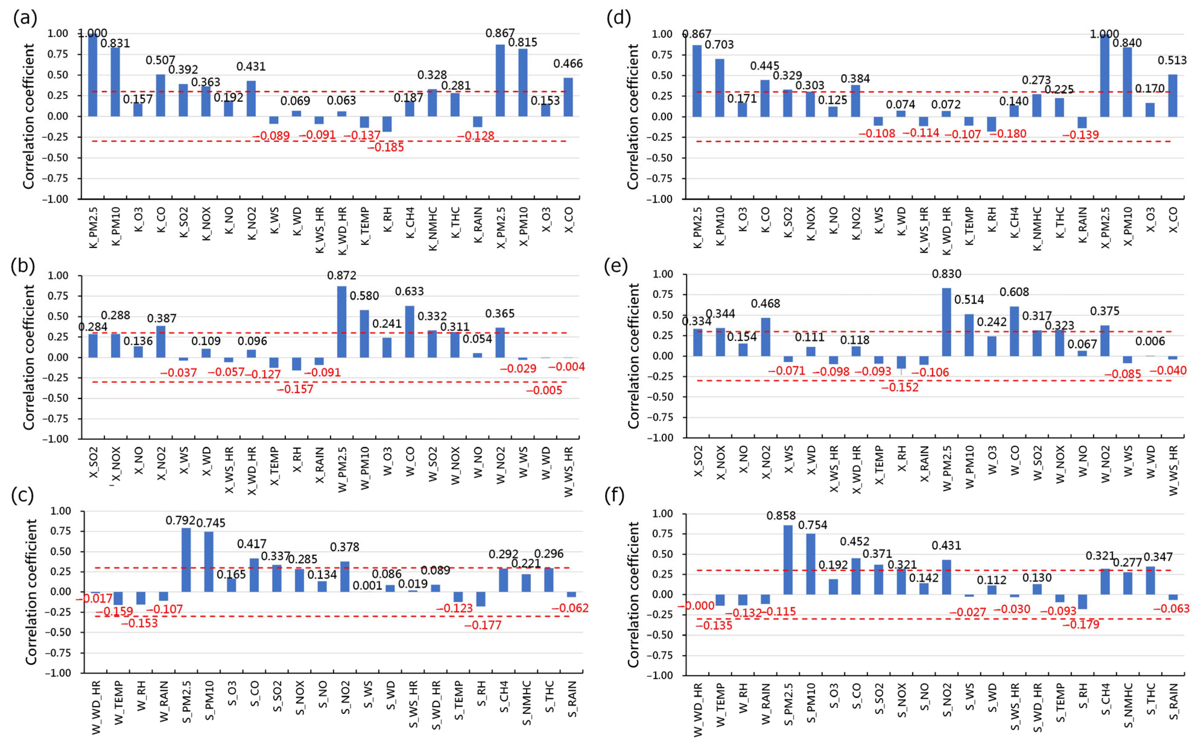
The consideration of regional variability in the relationships among meteorological factors, pollutants, and PM2.5 concentration has been discussed in detail in [28,29,30,31,32]. In response to concerns regarding the absence of meteorological parameters in the selected features, we conducted a correlation analysis to identify pertinent variables for our model. Specifically, this study employed correlation analysis to select suitable input variables for the target monitoring stations, namely, Keelung Station and Xizhi Station.
Following Taylor’s guidelines [46], where a correlation coefficient |r|≥ 0.3 is considered to indicate moderate to high correlation, and |r|< 0.3 indicates low correlation, we applied this criterion to determine the relevance of the attribute data to PM2.5 at each target station. In other words, we selected attributes based on whether the correlation coefficient between the attribute data and PM2.5 at each target station is greater than or equal to 0.3. This approach ensures that only attributes with a meaningful correlation are considered for inclusion in the model.
Figure 2 provide a visual representation of the correlation coefficients between various attributes and PM2.5 concentration in the target stations. As depicted in Table 2, Keelung Station and Xizhi Station selected 21 and 25 attributes, respectively. The results of the correlation analysis highlighted notable correlations, particularly observing high correlations for PM2.5, PM10, and CO at each station.

3.2. Calibration of Model Parameters

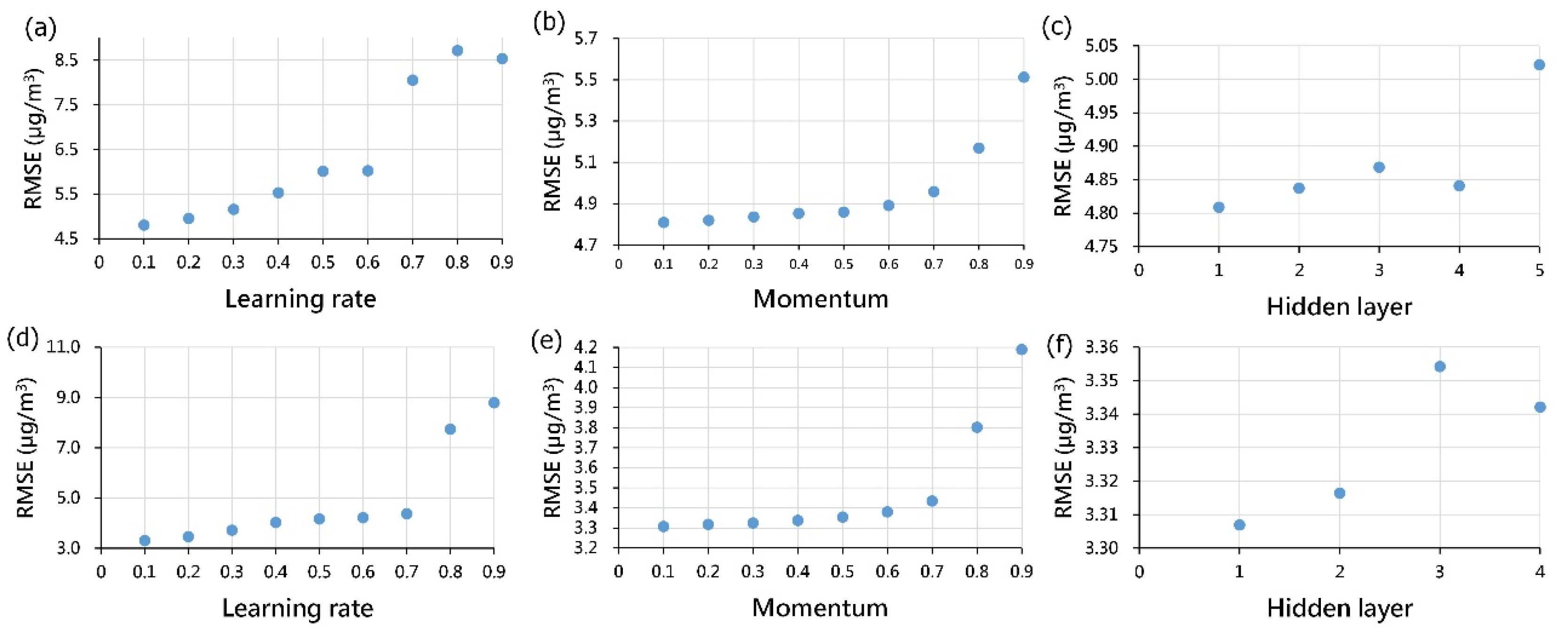
The parameter-tuning process for the DNN model encompasses adjustments to the learning rate, momentum, and the number of hidden layers. Specifically, the number of neurons in the hidden layer was determined following a recommendation from [35], where the parameter was set to ((input layer neurons + output layer neurons − 1)/2). To fine-tune these parameters, a trial-and-error method was applied at both the Keelung and Xizhi stations. Figure 3 illustrates the parameter tuning of the DNN model at forecasting time t + 1 for the learning rate, momentum, and the number of hidden layers. The figure indicates that, for the Keelung station, the optimal parameters are learning rate = 0.1, momentum = 0.1, and one hidden layer; similarly, for the Xizhi station, the optimal parameters are learning rate = 0.1, momentum = 0.1, and one hidden layer. Parameter tuning for the DNN model at forecasting time t + 2 to t + 12 can be obtained in the same manner.
The parameter to be tuned for the M5P model is the minimum number of instances for the target values (leaf nodes). This parameter determines the tree structure of the decision tree. Figure 4 illustrates the parameter tuning of the M5P model at forecasting time t + 1 for the minimum number instances. The figure indicates that the optimal parameters for the Keelung station and Xizhi station are minimum numbers of instances of 36 and 41, respectively. This parameter tuning for M5P and subsequent decision tree models (i.e., M5Rules and AMT) at time steps t + 2 to t + 12 can also be obtained in the same manner.
M5Rules is a model derived from M5P, differing only in certain pruning methods and the smoothing treatment of the target values (leaf nodes). The parameter to be tuned for the M5Rules model is also the minimum number of instances. Figure 5 illustrates the parameter tuning of the M5Rules model at forecasting time t + 1 for the minimum number instances. The figure indicates that the optimal parameters for the Keelung station and Xizhi station are minimum numbers of instances of 36 and 41, respectively.
The parameter in the AMT model is shrinkage, which can control the phenomenon of overfitting. Figure 6 illustrates the parameter tuning of the AMT model at forecasting time t + 1 for the shrinkage. The figure indicates that the optimal parameters for the Keelung station and Xizhi station are achieved when the shrinkage is set to 1.

3.3. Model Testing Results

This section employs a testing set to evaluate the model validated in the previous section. Table 3 shows the performance of these models for future hour predictions at Keelung Station. For t + 1 and t + 3, the M5P model performs the best, while DNN performs the worst. For t + 6, DNN performs the best, with M5P performing the worst. Finally, for t + 12, the M5Rules model performs the best, with DNN performing the worst. When comparing the performance of the models across different time horizons, DNN shows a strong performance for t + 1, t + 3, t + 6, and t + 12 compared to other models.
Table 4 presents the results of the tests conducted on Xizhi Station using the DNN, M5P, M5Rules, and AMT models. Among these models, M5Rules performed the best in predicting future hourly values at t + 1, t + 3, t + 6, and t + 12. MLR exhibited the poorest performance at t + 3, t + 6, and t + 12. DNN had the weakest performance at t + 12. Comparing the models’ correlation coefficients (r) at different future time intervals, it was observed that DNN performed best in predicting future values at t + 1 and t + 12. M5Rules excelled at t + 3 and t + 6. MLR performed the worst at t + 1, t + 3, t + 6, and t + 12. Notably, there was a slight difference in performance between the M5P and M5Rules models at t + 12.
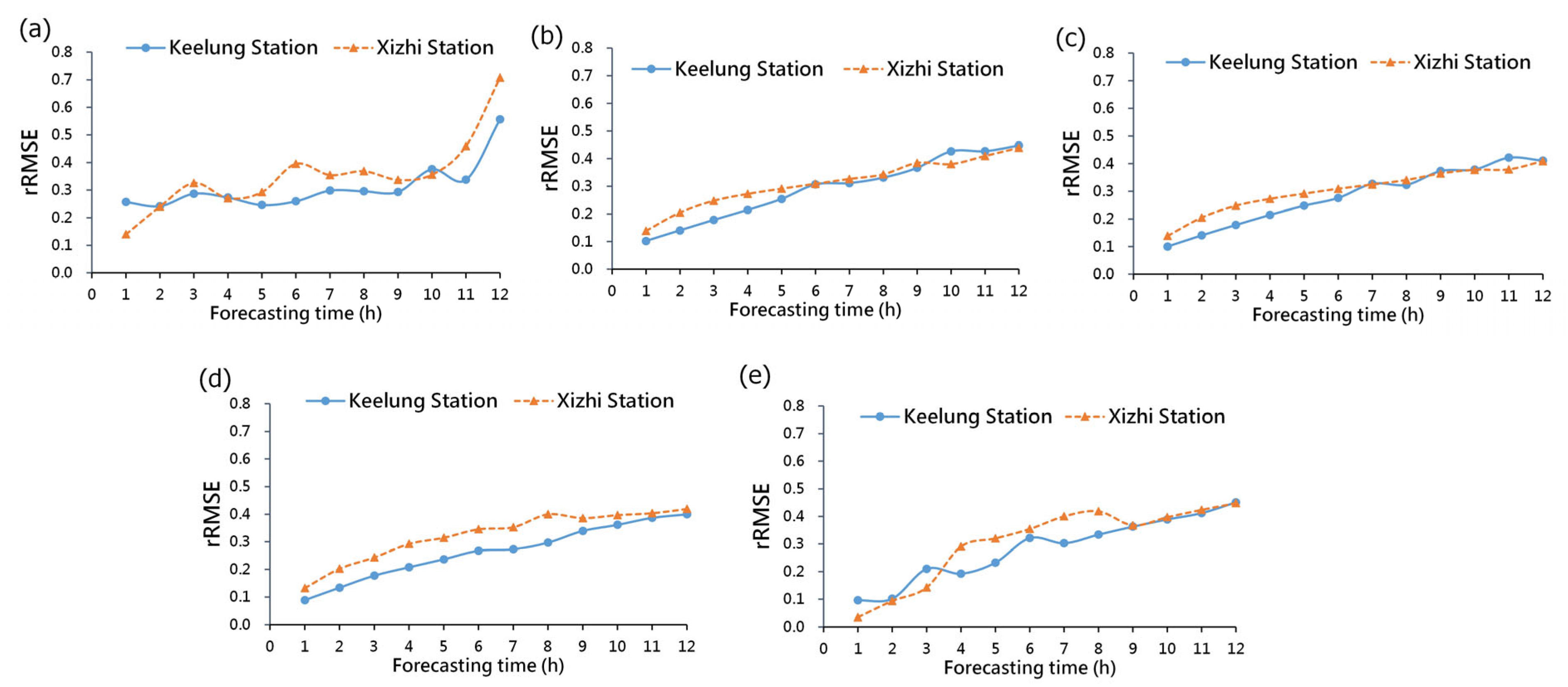
Figure 7 depicts the comparison of rRMSE between Keelung Station and Xizhi Station. In Figure 7a, it is evident that the DNN model exhibits greater fluctuations in rRMSE at both Keelung and Xizhi Stations compared to other models (M5P, M5Rules, AMT, and MLR in Figure 7b–e). Among them, the highest rRMSE is observed for the prediction of future time t + 12 at Xizhi Station, reaching 0.71. In contrast to the DNN and MLR models, decision tree-based models (M5P, M5Rules, and AMT) show a stable increase in rRMSE at both Keelung and Xizhi Stations as the prediction time horizons. The comprehensive analysis of predictive results indicates that no single model achieves overall optimal performance over the time horizons. This suggests that selecting different models for different prediction times can enhance prediction accuracy.

3.4. Model Comparison

As previously mentioned, no single model achieves optimal performance across all time horizons. This section delves into a comprehensive discussion and offers potential explanations for the varying performance levels observed in these models.
The strength of decision trees lies in their ability to represent rules, a characteristic that sets them apart from ANNs functioning more like black boxes. Decision trees allow for a clear expression of rules, enhancing human understanding. Furthermore, the determination of the relative importance of input parameters in ANNs necessitates a sensitivity analysis post ANN construction [47,48]. In contrast, decision trees autonomously identify crucial parameters through the branching of inputs. In the case of DNNs, establishing the optimal network structure, encompassing the number of hidden layers and neurons in each layer, is imperative. This process often entails trial and error, a time-consuming sequence of actions [49]. Conversely, decision trees are non-parametric and, thus, more convenient to use. In summary, the inherent differences in modeling between ANNs and decision trees may lead to varied feature extraction or an adverse effect caused by the use of excessive features in DNNs, contributing to different performance outcomes at different time horizons.

4. Simulation

4.1. A Real-Time Prediction System

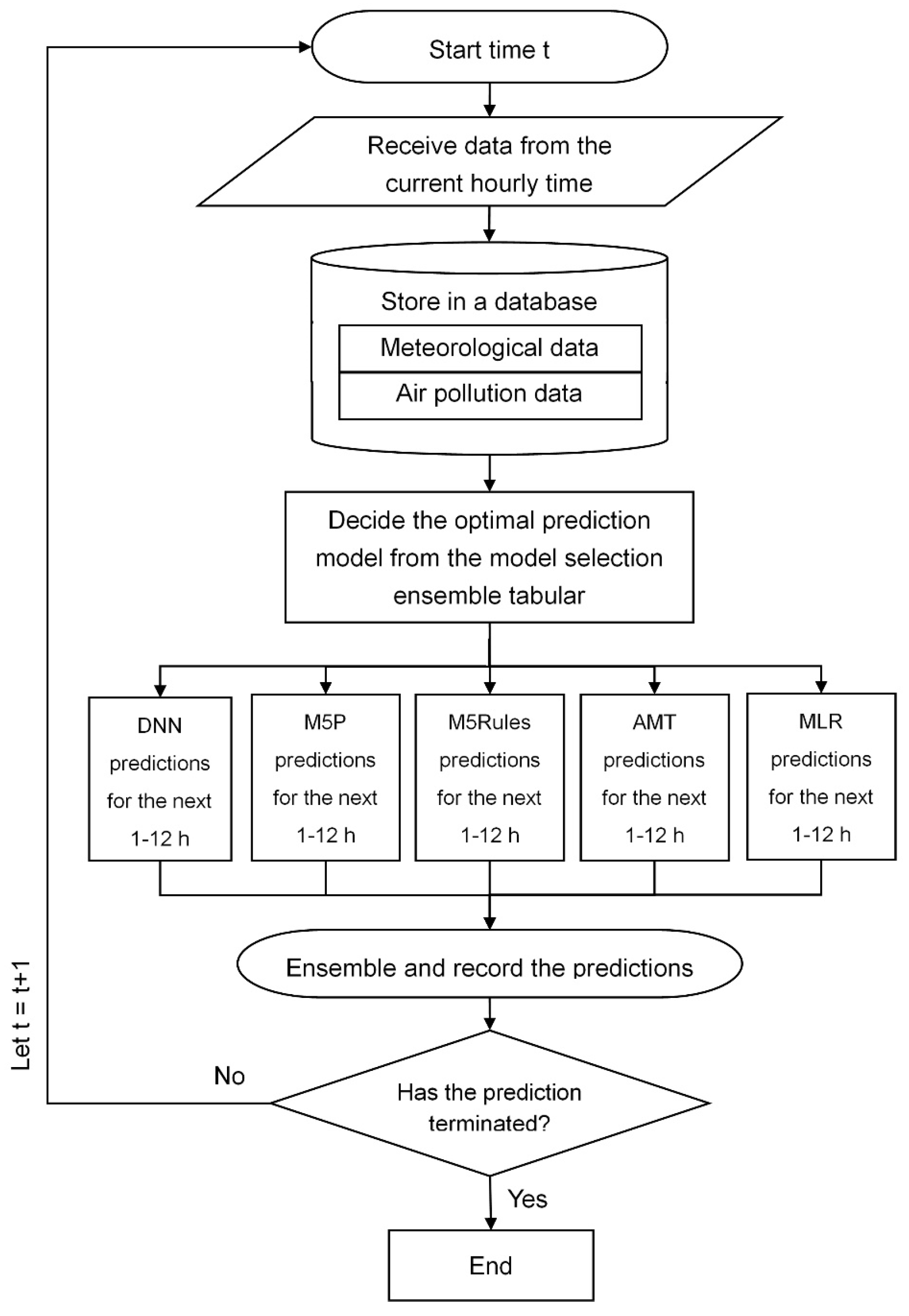
The real-time prediction system workflow is illustrated in Figure 8. The prediction system imports data into the database at the current hourly time, and selects the optimal prediction model for each future hour based on the mode selection ensemble tabular. By calculating the results of all models and combining the required prediction values, the system continues the prediction process until termination.
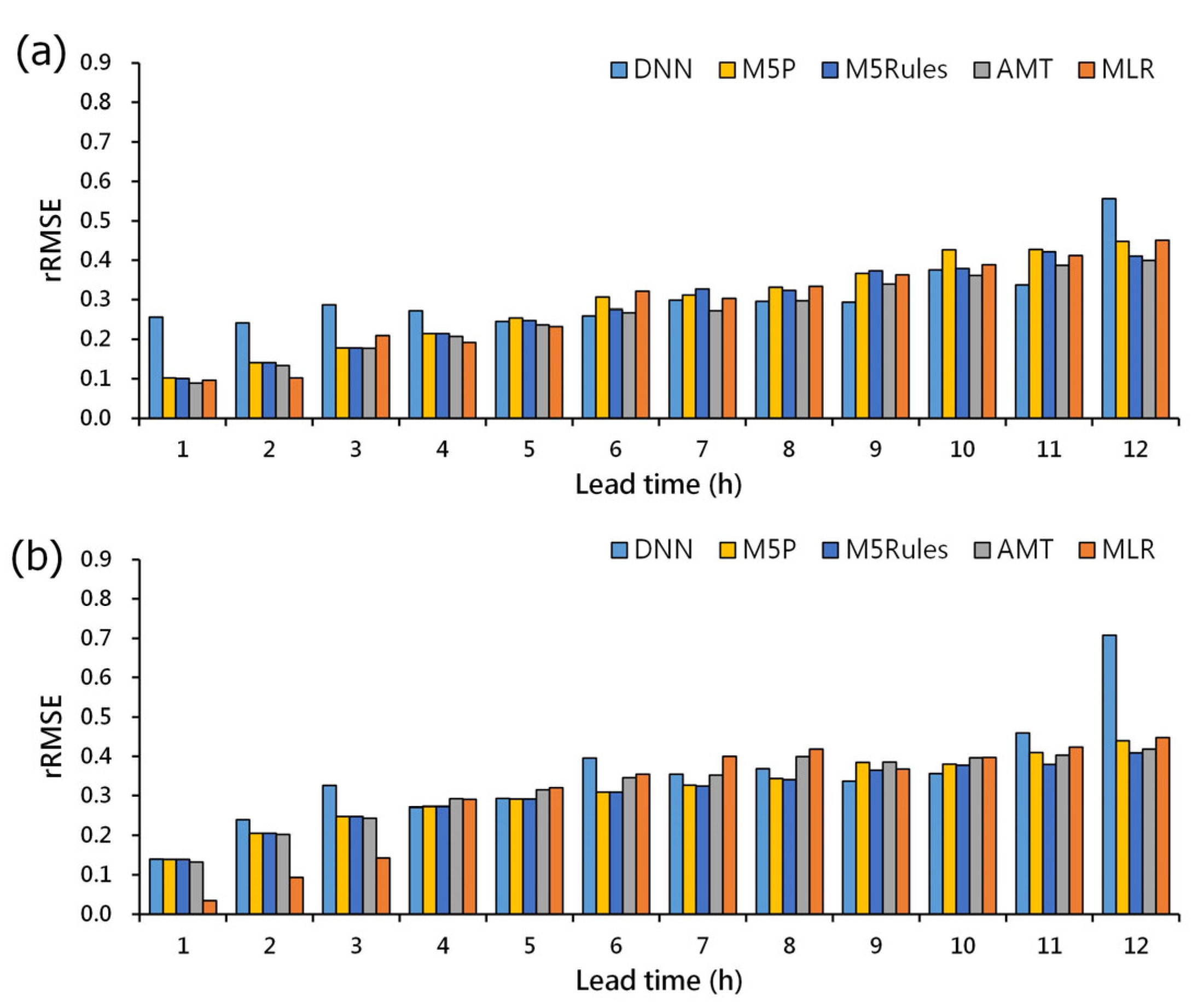
For the convenience of creating the model selection ensemble tabular, we transform Figure 7a–e into histograms displaying the rRMSE of the five models for each predicted time period simultaneously (as shown in Figure 9). Through Figure 9, we can quickly compile a table, referred to as the model selection ensemble tabular (as in Table 5), listing the optimal prediction model for each future prediction hour at both Keelung and Xizhi Stations.
Due to the prevalence of the northeasterly monsoon in the research area during the winter season, the developed real-time prediction system for PM2.5 concentration can be used to test the system’s performance during this specific season. Since the system’s construction is based on annual data, we established a separate real-time PM2.5 concentration prediction system specifically for the winter season. Table 6 presents the selection model ensemble tabular for the winter season.

4.2. System Simulations

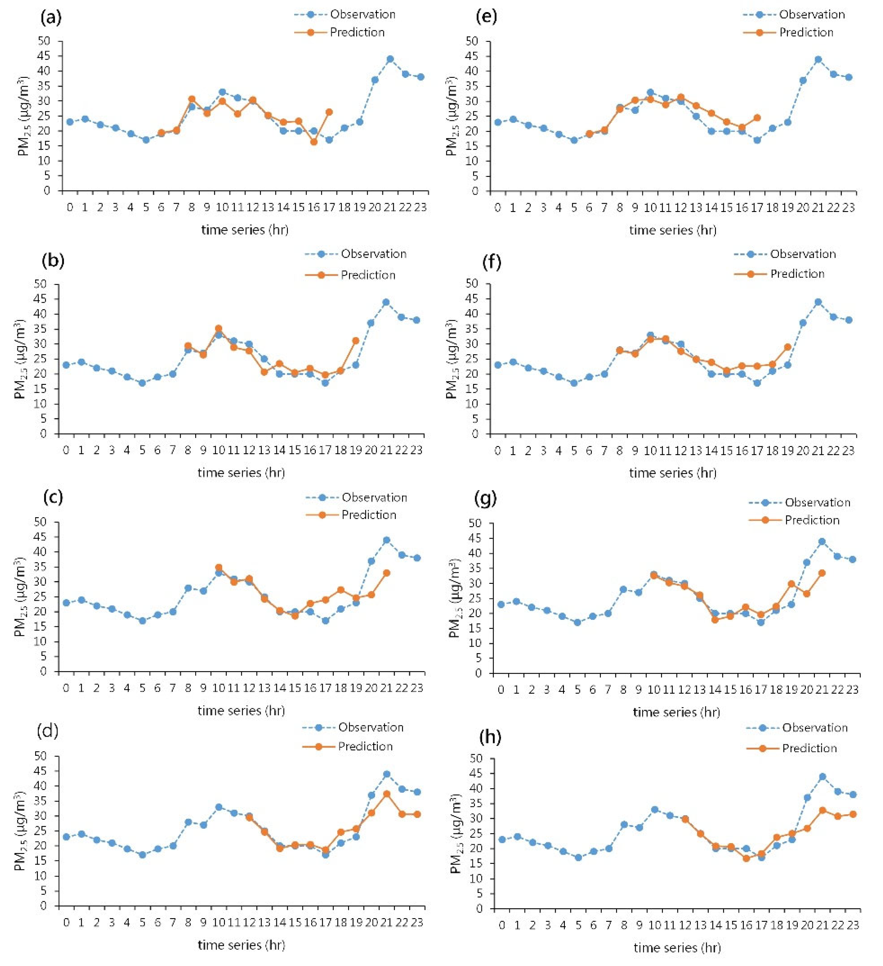
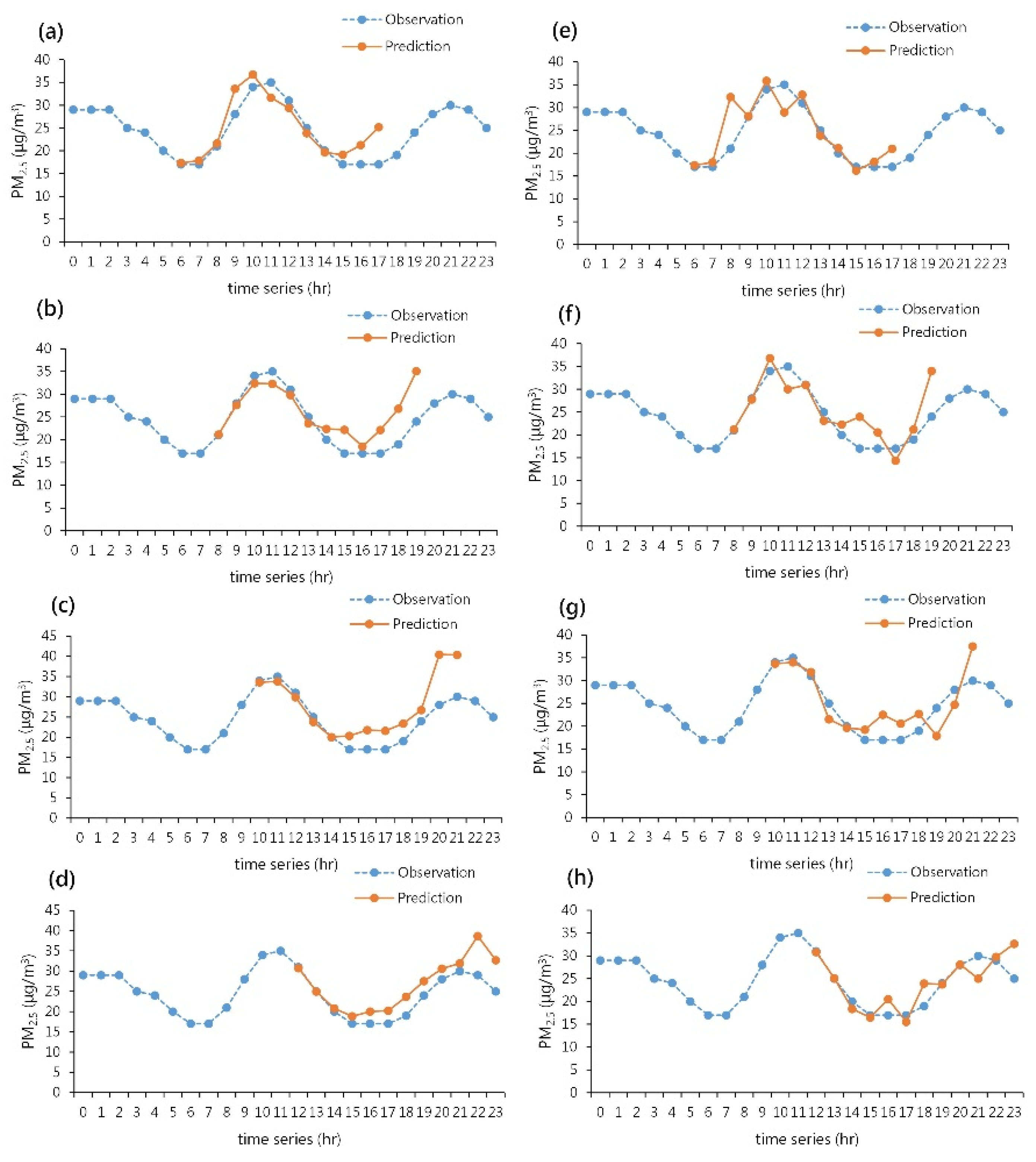
Figure 10 and Figure 11 show the real-time prediction results of the forecasting system for Keelung Station and Xizhi Station, respectively, using 6 February 2022 as an example. Figure 10a–d present the real-time prediction system for annual data, while Figure 11a–d depict the real-time prediction system for the winter season. In both sets of figures, the blue dashed lines represent the observed values of PM2.5, and the orange solid lines represent the predictions generated by the system. Each prediction period covers the next 12 h from the current moment. The predictions start at 5 AM on the given day and are adjusted hourly for fine particulate matter values. Figure 10d,h indicate that Keelung Station underestimated the values starting from 11 AM, continuing into the evening at 8 PM. On the other hand, Xizhi Station showed a slight overestimation, as seen in Figure 11d,h. Overall, the real-time prediction systems for both annual data and the winter season data at Keelung Station and Xizhi Station demonstrate the changing trends in fine particulate matter concentrations.

5. Conclusions

This study has established machine-learning models for predicting fine particulate matter concentration and developed a real-time fine particulate matter prediction system. This system allows the public to obtain forecasts of future fine particulate matter concentrations before going outdoors. The system can adjust the predictions hourly over time to assist the public in understanding the changes in future fine particulate matter concentration. The study area includes Keelung City and Xizhi District in New Taipei City, Taiwan, and it predicts fine particulate matter concentrations for the next 1 to 12 h.
This study established five different fine particulate matter concentration prediction models, including DNN, M5P, M5Rules, AMT, and MLR. Based on the prediction results, it was found that no single model achieved comprehensive optimal performance in long-term forecasting. Therefore, this study used the above-mentioned models as a basis to build a real-time prediction system.
This study calculated the prediction results from the five different models and the real-time prediction system. From these analyses, the following conclusions were drawn:
(1)
When comparing different models, it was observed that decision tree models provided a more stable predictive performance across both Keelung Station and Xizhi Station. In contrast, the DNN model exhibited larger fluctuations in error values compared to other models across various prediction time horizons. The MLR model also displayed greater fluctuations in prediction errors at Xizhi Station compared to other models. However, it is worth noting that the DNN and MLR models outperformed other models in certain time horizons, indicating that each model has its own strengths and weaknesses in prediction.
(2)
If the PM2.5 concentration remains above 35 μg/m3 for an extended period, there is a higher probability that the predicted results will be underestimated. The main reason for this may be the infrequent occurrence of high concentrations in historical data, causing the model to be ineffective in predicting high values.
(3)
At different prediction time horizons, all models performed well in predicting results for the next 3 h. However, the prediction errors began to increase for predictions in the 4 to 6 h range. For longer-term predictions covering 12 h, all models exhibited larger prediction errors. In general, as the prediction time interval increased, the prediction errors also increased, indicating that longer-term forecasts are more challenging for all models.
(4)
Ultimately, this study developed a real-time fine particulate matter concentration prediction system that can predict the changes in fine particulate matter concentration for the next 12 h. The system also includes hourly adjustments to the predictions. Compared to the performance of individual models, the real-time prediction system provides a more comprehensive and accurate prediction trend.

Author Contributions

C.-C.W. conceived and designed the experiments and wrote the manuscript, and W.-J.K. and C.-C.W. carried out this experiment and analysis of the data and discussed the results. All authors have read and agreed to the published version of the manuscript.

Funding

This research was funded by the Ministry of Science and Technology, Taiwan, grant number NSTC112-2622-M-019-001.

Institutional Review Board Statement

Not applicable.

Informed Consent Statement

Not applicable.

Data Availability Statement

The related data were provided by the air quality monitoring website of Taiwan’s Ministry of Environment, which are available at https://airtw.moenv.gov.tw/ (accessed on 1 December 2022).

Acknowledgments

The author acknowledges the data provided by Taiwan’s Ministry of Environment.

Conflicts of Interest

Wei-Jen Kao is an employee of Wisdom Environmental Technical Service and Consultant Company. Wei-Jen Kao was funded by Wisdom Environmental Technical Service and Consultant Company. The company had no roles in the design of the study; in the collection, analysis, or interpretation of data; in the writing of the manuscript, or in the decision to publish the articles. The paper reflects the views of the scientists and not the company. The authors declare no conflict of interest.

References

  1. Kong, S.; Li, X.; Li, L.; Yin, Y.; Chen, K.; Yuan, L.; Zhang, Y.; Shan, Y.; Ji, Y. Variation of polycyclic aromatic hydrocarbons in atmospheric PM2.5 during winter haze period around 2014 Chinese Spring Festival at Nanjing: Insights of source changes, air mass direction and firework particle injection. Sci. Total Environ. 2015, 520, 59–72. [Google Scholar] [CrossRef] [PubMed]
  2. Alvarez, H.A.O.; Myers, O.B.; Weigel, M.; Armijos, R.X. The value of using seasonality and meteorological variables to model intra-urban PM2.5 variation. Atmos. Environ. 2018, 182, 1–8. [Google Scholar] [CrossRef] [PubMed]
  3. Tai, A.P.; Mickley, L.J.; Jacob, D.J. Correlations between fine particulate matter (PM2.5) and meteorological variables in the United States: Implications for the sensitivity of PM2.5 to climate change. Atmos. Environ. 2010, 44, 3976–3984. [Google Scholar] [CrossRef]
  4. Li, L.; Qian, J.; Ou, C.Q.; Zhou, Y.X.; Guo, C.; Guo, Y. Spatial and temporal analysis of Air Pollution Index and its timescale-dependent relationship with meteorological factors in Guangzhou, China, 2001–2011. Environ. Pollut. 2014, 190, 75–81. [Google Scholar] [CrossRef] [PubMed]
  5. Shah, A.S.V.; Langrish, J.P.; Nair, H.; McAllister, D.A.; Hunter, A.L.; Donaldson, K.; Newby, D.E.; Mills, N.L. Global association of air pollution and heart failure: A systematic review and meta-analysis. Lancet 2013, 382, 1039–1048. [Google Scholar] [CrossRef] [PubMed]
  6. Srimuruganandam, B.; Nagendra, S.S. Source characterization of PM10 and PM2.5 mass using a chemical mass balance model at urban roadside. Sci. Total Environ. 2012, 433, 8–19. [Google Scholar] [CrossRef]
  7. Atkinson, R.W.; Fuller, G.W.; Anderson, H.R.; Harrison, R.M.; Armstrong, B. Urban ambient particle metrics and health: A time-series analysis. Epidemiology 2010, 21, 501–511. [Google Scholar] [CrossRef]
  8. Brauer, M.; Amann, M.; Burnett, R.T.; Cohen, A.; Dentener, F.; Ezzati, M.; Henderson, S.B.; Krzyzanowski, M.; Martin, R.V.; Van Dingenen, R.; et al. Exposure assessment for estimation of the global burden of disease attributable to outdoor air pollution. Environ. Sci. Technol. 2012, 46, 652–660. [Google Scholar] [CrossRef]
  9. Cheung, K.; Daher, N.; Kam, W.; Shafer, M.M.; Ning, Z.; Schauer, J.J.; Sioutas, C. Spatial and temporal variation of chemical composition and mass closure of ambient coarse particulate matter (PM10–2.5) in the Los Angeles area. Atmos. Environ. 2011, 45, 2651–2662. [Google Scholar] [CrossRef]
  10. Yang, F.; Tan, J.; Zhao, Q.; Du, Z.; He, K.; Ma, Y.; Duan, F.; Chen, G.; Zhao, Q. Characteristics of PM2.5 speciation in representative megacities and across China. Atmos. Chem. Phys. 2011, 11, 5207–5219. [Google Scholar] [CrossRef]
  11. Zhang, Y. Dynamic effect analysis of meteorological conditions on air pollution: A case study from Beijing. Sci. Total Environ. 2019, 684, 178–185. [Google Scholar] [CrossRef] [PubMed]
  12. Ni, X.Y.; Huang, H.; Du, W.P. Relevance analysis and short-term prediction of PM2.5 concentrations in Beijing based on multi-source data. Atmos. Environ. 2017, 150, 146–161. [Google Scholar] [CrossRef]
  13. Anagnostopoulos, F.K.; Rigas, S.; Papachristou, M.; Chaniotis, I.; Anastasiou, I.; Tryfonopoulos, C.; Raftopoulou, P. A novel AI framework for PM pollution prediction applied to a Greek Port City. Atmosphere 2023, 14, 1413. [Google Scholar] [CrossRef]
  14. Lai, K.; Xu, H.; Sheng, J.; Huang, Y. Hour-by-hour prediction model of air pollutant concentration based on EIDW-informer—A case study of Taiyuan. Atmosphere 2023, 14, 1274. [Google Scholar] [CrossRef]
  15. Liu, X.; Zhao, K.; Liu, Z.; Wang, L. PM2.5 Concentration prediction based on LightGBM optimized by adaptive multi-strategy enhanced sparrow search algorithm. Atmosphere 2023, 14, 1612. [Google Scholar] [CrossRef]
  16. Mampitiya, L.; Rathnayake, N.; Leon, L.P.; Mandala, V.; Azamathulla, H.M.; Shelton, S.; Hoshino, Y.; Rathnayake, U. Machine learning techniques to predict the air quality using meteorological data in two urban areas in Sri Lanka. Environments 2023, 10, 141. [Google Scholar] [CrossRef]
  17. Corani, G. Air quality prediction in Milan: Feed-forward neural networks, pruned neural networks and lazy learning. Ecol. Model. 2005, 185, 513–529. [Google Scholar] [CrossRef]
  18. Bai, Y.; Li, Y.; Wang, X.; Xie, J.; Li, C. Air pollutants concentrations forecasting using back propagation neural network based on wavelet decomposition with meteorological conditions. Atmos. Pollut. Res. 2016, 7, 557–566. [Google Scholar] [CrossRef]
  19. Siwek, K.; Osowski, S. Data mining methods for prediction of air pollution. Int. J. Appl. Math. Comput. Sci. 2016, 26, 467–478. [Google Scholar] [CrossRef]
  20. Li, C.; Zhu, Z. Research and application of a novel hybrid air quality early-warning system: A case study in China. Sci. Total Environ. 2018, 626, 1421–1438. [Google Scholar] [CrossRef]
  21. Mehdipour, V.; Stevenson, D.S.; Memarianfard, M.; Sihag, P. Comparing different methods for statistical modeling of particulate matter in Tehran, Iran. Air Qual. Atmos. Health 2018, 11, 1155–1165. [Google Scholar] [CrossRef]
  22. Wang, J.; Song, G. A deep spatial-temporal ensemble model for air quality prediction. Neurocomputing 2018, 314, 198–206. [Google Scholar] [CrossRef]
  23. Lee, M.; Lin, L.; Chen, C.Y.; Tsao, Y.; Yao, T.H.; Fei, M.H.; Fang, S.H. Forecasting air quality in Taiwan by using machine learning. Sci. Rep. 2020, 10, 4153. [Google Scholar] [CrossRef] [PubMed]
  24. Ma, X.; Chen, T.; Ge, R.; Xv, F.; Cui, C.; Li, J. Prediction of PM2.5 concentration using spatiotemporal data with machine learning models. Atmosphere 2023, 14, 1517. [Google Scholar] [CrossRef]
  25. Dai, H.; Huang, G.; Wang, J.; Zeng, H. VAR-tree model based spatio-temporal characterization and prediction of O3 concentration in China. Ecotoxicol. Environ. Saf. 2023, 257, 114960. [Google Scholar] [CrossRef] [PubMed]
  26. Dai, H.; Huang, G.; Zeng, H. Multi-objective optimal dispatch strategy for power systems with Spatio-temporal distribution of air pollutants. Sustain. Cities Soc. 2023, 98, 104801. [Google Scholar] [CrossRef]
  27. Liu, C.M.; Young, C.Y.; Lee, Y.C. Influence of Asian dust storms on air quality in Taiwan. Sci. Total Environ. 2006, 368, 884–897. [Google Scholar] [CrossRef]
  28. Misra, C.; Geller, M.D.; Shah, P.; Sioutas, C.; Solomon, P.A. Development and Evaluation of a Continuous Coarse (PM10–PM2.5) Particle Monitor. J. Air Waste Manag. Assoc. 2001, 51, 1309–1317. [Google Scholar] [CrossRef]
  29. Juda-Rezler, K.; Reizer, M.; Oudinet, J.P. Determination and analysis of PM10 source apportionment during episodes of air pollution in Central Eastern European urban areas: The case of wintertime 2006. Atmos. Environ. 2011, 45, 6557–6566. [Google Scholar] [CrossRef]
  30. Liu, Y.; Zhao, N.; Vanos, J.K.; Cao, G. Effects of synoptic weather on ground-level PM2.5 concentrations in the United States. Atmos. Environ. 2017, 148, 297–305. [Google Scholar] [CrossRef]
  31. Zhang, R.; Jing, J.; Tao, J.; Hsu, S.-C.; Wang, G.; Cao, J.; Lee, C.S.L.; Zhu, L.; Chen, Z.; Zhao, Y.; et al. Chemical characterization and source apportionment of PM2.5 in Beijing: Seasonal perspective. Atmos. Chem. Phys. Discuss. 2013, 13, 9953–10007. [Google Scholar]
  32. Hsu, C.H.; Cheng, F.Y. Synoptic weather patterns and associated air pollution in Taiwan. Aerosol Air Qual. Res. 2019, 19, 1139–1151. [Google Scholar] [CrossRef]
  33. De Villiers, J.; Barnard, E. Backpropagation neural nets with one and two hidden layers. IEEE Trans. Neural Netw. 1993, 4, 136–141. [Google Scholar] [CrossRef] [PubMed]
  34. Kwok, T.Y.; Yeung, D.Y. Constructive algorithms for structure learning in feedforward neural networks for regression problems. IEEE Trans. Neural Netw. 1997, 8, 630–645. [Google Scholar] [CrossRef] [PubMed]
  35. Trenn, S. Multilayer perceptrons: Approximation order and necessary number of hidden units. IEEE Trans. Neural Netw. 2008, 19, 836–844. [Google Scholar] [CrossRef] [PubMed]
  36. Chien, C.F.; Chen, L.F. Data mining to improve personnel selection and enhance human capital: A case study in high-technology industry. Expert Syst. Appl. 2008, 34, 280–290. [Google Scholar] [CrossRef]
  37. Wang, Y.; Witten, I.H. Induction of Model Trees for Predicting Continuous Classes; Working Paper 96/23; University of Waikato, Department of Computer Science: Hamilton, New Zealand, 1996. [Google Scholar]
  38. Quinlan, J.R. Learning with continuous classes. In Proceedings of the 5th Australian Joint Conference on Artificial Intelligence, Hobart, Australia, 16–18 November 1992; pp. 343–348. [Google Scholar]
  39. Breiman, L.; Friedman, J.; Stone, C.J.; Olshen, R.A. Classification and Regression Trees; CRC Press: Boca Raton, FL, USA, 1984. [Google Scholar]
  40. Holmes, G.; Hall, M.; Prank, E. Generating rule sets from model trees. In Proceedings of the Australasian Joint Conference on Artificial Intelligence, Sydney, Australia, 6–10 December 1999; pp. 1–12. [Google Scholar]
  41. Jaakkola, H.; Thalheim, B.; Kiyoki, Y.; Yoshida, N. (Eds.) Information Modelling and Knowledge Bases XXVIII; Frontiers in Artificial Intelligence and Applications; IOS Press: Amsterdam, The Netherlands, 2017; Volume 292. [Google Scholar]
  42. Holmes, G.; Pfahringer, B.; Kirkby, R.; Frank, E.; Hall, M. Multiclass alternating decision trees. In Proceedings of the European Conference on Machine Learning, Helsinki, Finland, 19–23 August 2002; pp. 161–172. [Google Scholar]
  43. Frank, E.; Mayo, M.; Kramer, S. Alternating model trees. In Proceedings of the 30th Annual ACM Symposium on Applied Computing, Salamanca, Spain, 13–17 April 2015; pp. 871–878. [Google Scholar]
  44. Freund, Y.; Mason, L. The alternating decision tree learning algorithm. In Proceedings of the Sixteenth International Conference on Machine Learning, Bled, Slovenia, 27–30 June 1999; pp. 124–133. [Google Scholar]
  45. Montgomery, D.C.; Peck, E.A.; Vining, G.G. Introduction to Linear Regression Analysis; John Wiley & Sons: Hoboken, NJ, USA, 2012; Volume 821. [Google Scholar]
  46. Taylor, R. Interpretation of the correlation coefficient: A basic review. J. Diagn. Med. Sonogr. 1990, 6, 35–39. [Google Scholar] [CrossRef]
  47. Mahjoobi, J.; Etemad-Shahidi, A.; Kazeminezhad, M.H. Hindcasting of wave parameters using different soft computing methods. Appl. Ocean Res. 2008, 30, 28–36. [Google Scholar] [CrossRef]
  48. Tso, G.K.F.; Yau, K.K.W. Predicting electricity energy consumption: A comparison of regression analysis, decision tree and neural networks. Energy 2007, 32, 1761–1768. [Google Scholar] [CrossRef]
  49. Mahjoobi, J.; Etemad-Shahidi, A. An alternative approach for the prediction of significant wave heights based on classification and regression trees. Appl. Ocean. Res. 2008, 30, 172–177. [Google Scholar] [CrossRef]
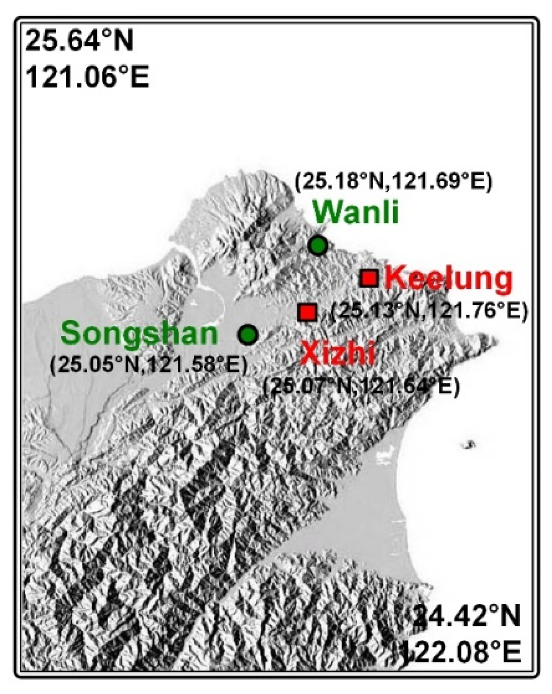
Figure 1. Location of the study area and stations.
Atmosphere 14 01817 g001
Figure 2. Correlation coefficients of various attributes with PM2.5 concentration in the target stations: (ac) for Keelung Station; and (df) for Xizhi Station. In the figure, variables with the prefix “K_” denote Keelung Station, “X_” represents Xizhi Station, “W_” corresponds to Wanli Station, and “S_” indicates Songshan Station.
Atmosphere 14 01817 g002
Figure 3. Parameter calibration of the DNN model: (ac) Keelung Station; and (df) Xizhi Station.
Atmosphere 14 01817 g003
Figure 4. Parameter calibration of the M5P model: (a) Keelung Station; and (b) Xizhi Station.
Atmosphere 14 01817 g004
Figure 5. Parameter calibration of the M5Rules model: (a) Keelung Station; and (b) Xizhi Station.
Atmosphere 14 01817 g005
Figure 6. Parameter calibration of the AMT model: (a) Keelung Station; and (b) Xizhi Station.
Atmosphere 14 01817 g006
Figure 7. Comparison of rRMSE for 1 to 12 h forecasts at Keelung and Xizhi Stations: (a) DNN; (b) M5P; (c) M5Rules; (d) AMT; and (e) MLR.
Atmosphere 14 01817 g007
Figure 8. A real-time forecasting system.
Atmosphere 14 01817 g008
Figure 9. Histograms of rRMSE for 1–12 h predictions: (a) Keelung Station; and (b) Xizhi Station.
Atmosphere 14 01817 g009
Figure 10. The real-time prediction system simulation results for Keelung Station: (ad) for the annual prediction system, and (eh) for the winter seasonal prediction system.
Atmosphere 14 01817 g010
Figure 11. The real-time prediction system simulation results for Xizhi Station: (ad) for the annual prediction system, and (eh) for the winter seasonal prediction system.
Atmosphere 14 01817 g011
Table 1. Air quality monitoring stations and their parameters.
StationMonitoring Parameters
KeelungAMB_TEMP, WIND_SPEED, WIND_DIREC, WS_HR, WD_HR, RAINFALL, RH, PM2.5, PM10, O3, SO2, CO, NOX, NO, NO2, THC, CH4, NMHC
XizhiAMB_TEMP, WIND_SPEED, WIND_DIREC, WS_HR, WD_HR, RAINFALL, RH, PM2.5, PM10, O3, SO2, CO, NOX, NO, NO2
WanliAMB_TEMP, WIND_SPEED, WIND_DIREC, WS_HR, WD_HR, RAINFALL, RH, PM2.5, PM10, O3, SO2, CO, NOX, NO, NO2
SongshanAMB_TEMP, WIND_SPEED, WIND_DIREC, WS_HR, WD_HR, RAINFALL, RH, PM2.5, PM10, O3, SO2, CO, NOX, NO, NO2, THC, CH4, NMHC
Table 2. Selected attributes for each target station.
Target StationSelected Attributes
KeelungPM2.5, PM10, SO2, CO, NOX, NO2, and NMHCW of Keelung Station; PM2.5, PM10, CO, and NO2 of Xizhi Station; PM2.5, PM10, SO2, CO, and NO2 of Wanli Station; PM2.5, PM10, SO2, CO, and NO2 of Songshan Station
XizhiPM2.5, PM10, SO2, CO, and NO2 of Keelung Station; PM2.5, PM10, SO2, CO, NOX, and NO2 of Xizhi Station; PM2.5, PM10, SO2, CO, NOX, and NO2 of Wanli Station; PM2.5, PM10, SO2, CO, NOX, NO2, THC, and CH4 of Songshan Station
Table 3. Performance levels at time horizons of 1 to 12 h for Keelung Station.
Lead Time (h)PerformanceDNNM5PM5RulesAMTMLR
t + 1RMSE (μg/m3)5.223.993.993.994.00
MAPE16.1012.0613.4011.7216.10
CE0.820.870.840.870.82
r0.920.910.910.910.91
t + 3RMSE (μg/m3)6.655.965.966.026.05
MAPE19.6217.7418.5218.8719.62
CE0.760.820.810.770.76
r0.810.810.810.800.81
t + 6RMSE (μg/m3)7.187.687.497.577.63
MAPE21.1422.9321.6422.8821.14
CE0.730.700.710.710.74
r0.680.670.680.670.68
t + 12RMSE (μg/m3)10.289.138.898.918.98
MAPE35.7832.1031.5632.0735.78
CE0.580.610.600.620.58
r0.540.510.530.530.53
Table 4. Performance levels at time horizons of 1 to 12 h for Xizhi Station.
Lead Time (h)PerformanceDNNM5PM5RulesAMTMLR
t + 1RMSE (μg/m3)2.612.592.592.673.08
MAPE10.6310.389.729.1710.63
CE0.870.870.860.870.87
r0.970.970.970.970.96
t + 3RMSE (μg/m3)5.615.215.215.355.92
MAPE19.5319.1318.7519.1819.53
CE0.760.820.780.770.76
r0.880.880.880.870.85
t + 6RMSE (μg/m3)7.616.976.977.348.37
MAPE25.9123.4525.1125.9825.91
CE0.670.710.690.690.67
r0.780.780.780.760.68
t + 12RMSE (μg/m3)9.939.198.849.039.86
MAPE38.1536.2836.3136.2138.15
CE0.490.500.520.530.49
r0.650.600.640.610.60
Table 5. Annual model selection ensemble tabular.
Lead Time (h)Keelung StationXizhi Station
t + 1AMTMLR
t + 2MLRMLR
t + 3AMTMLR
t + 4MLRM5P, M5Rules
t + 5MLRM5P, M5Rules
t + 6DNNM5P, M5Rules
t + 7AMTM5P
t + 8AMTM5P, M5Rules
t + 9DNNDNN
t + 10AMTDNN
t + 11DNNAMT
t + 12AMTAMT
Table 6. The model selection ensemble tabular for winter season.
Lead Time (h)Keelung StationXizhi Station
t + 1MLRMLR
t + 2MLRMLR
t + 3MLRM5P, M5Rules
t + 4M5P, M5RulesDNN
t + 5DNNM5P
t + 6DNNDNN
t + 7AMTM5Rules
t + 8AMTDNN
t + 9AMTDNN
t + 10AMTDNN
t + 11DNNDNN
t + 12AMTM5Rules
Disclaimer/Publisher’s Note: The statements, opinions and data contained in all publications are solely those of the individual author(s) and contributor(s) and not of MDPI and/or the editor(s). MDPI and/or the editor(s) disclaim responsibility for any injury to people or property resulting from any ideas, methods, instructions or products referred to in the content.