Article

A Hybrid Model for Spatiotemporal Air Quality Prediction Based on Interpretable Neural Networks and a Graph Neural Network

1
Department of Computer Information Engineering, Cheongju University, Cheongju 28503, Republic of Korea
2
Division of Software Convergence, Cheongju University, Cheongju 28503, Republic of Korea
*
Author to whom correspondence should be addressed.
Atmosphere 2023, 14(12), 1807; https://doi.org/10.3390/atmos14121807
Submission received: 25 October 2023 / Revised: 5 December 2023 / Accepted: 7 December 2023 / Published: 9 December 2023
(This article belongs to the Section Atmospheric Techniques, Instruments, and Modeling)

Abstract

:
To effectively address air pollution and enhance air quality, governments must be able to predict the air quality index with high accuracy and reliability. However, air quality prediction is subject to ambiguity and instability because of the atmosphere’s fluidity, making it challenging to identify the temporal and spatial correlations using a single model. Therefore, a new hybrid model is proposed based on an interpretable neural network and a graph neural network (INNGNN), which simulates the temporal and spatial dependence of air quality and achieves accurate multi-step air quality prediction. A time series is first interpreted using interpretable neural networks (INN) to extract the potentially important aspects that are easily overlooked in the data; second, a self-attention mechanism catches the local and global dependencies and associations in the time series. Lastly, a city map is created using a graph neural network (GNN) to determine the relationships between cities in order to extract the spatially dependent features. In the experimental evaluation, the results show that the INNGNN model performs better than comparable algorithms. Therefore, it is confirmed that the INNGNN model can effectively capture the temporal and spatial relationships and better predict air quality.

1. Introduction

Human health and ecosystems depend heavily on the air quality, and air pollution is becoming a major global issue [1]. The term “air quality” refers to the quantity and make-up of several pollutants found in the atmosphere, including carbon monoxide, sulfur dioxide, nitrogen dioxide, PM2.5, PM10, and others. It is calculated based on the level of pollutant concentration and the degree of health impact, and is used to measure the air quality index (AQI). In addition to causing respiratory illnesses, air pollution has a negative impact on human health [2]; moreover, it also damages the environment and leads to an imbalance in the ecosystem [3]. The higher the AQI value, the worse the air quality. The air quality index (AQI) is a crucial metric that can help people understand that day’s air quality and take the appropriate precautions to safeguard their health. Additionally, pollutants can lower the AQI value and preserve the ecosystem’s equilibrium.
Air quality forecasting is a technique for predicting future air quality. This technology uses professional monitoring equipment and technology to collect and analyze atmospheric parameters (such as temperature, humidity, wind speed, air pressure, precipitation, etc.), geographical location, the air quality index, and other data, to predict and warn about air quality in the future [4]. The accurate prediction of AQI is crucial for safeguarding public health and maintaining ecosystem balance. However, air quality prediction (AQP) remains a challenging task due to complex temporal and spatial dependencies:
  • Temporal dependence. Periodicity and trend are the primary ways in which dynamic changes in air quality over time are expressed. Periodicity is the occurrence of similar patterns or regular changes over a certain span of time. As shown in Figure 1a, the air quality index changes periodically over a week (① indicates a period of change). Trend is when a certain data pattern shows a continuous directional development over a certain period of time. Figure 1a shows a downward trend on certain days and for a certain period of time with cyclical changes. As shown in Figure 1b, the air quality index over a day changes with time (② indicates a shift in the trend over a certain amount of time); for instance, air pollutants from a prior or longer period of time have an impact on the current AQI.
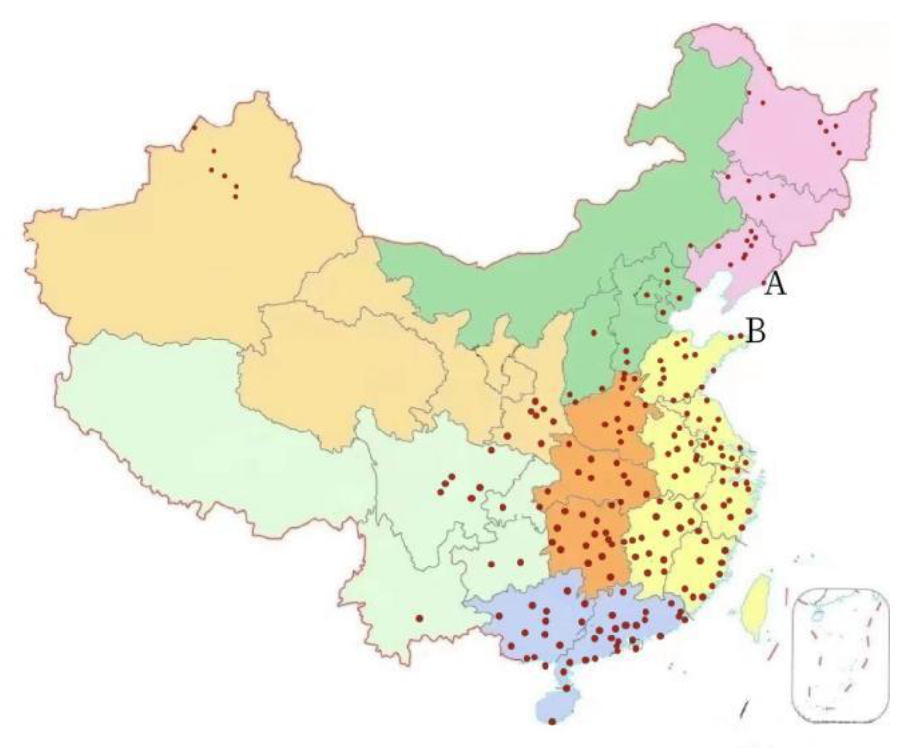
  • Complex spatiotemporal correlations. In addition to changing dynamically over time, the spatial location also has an impact on air quality. As illustrated in Figure 2, city B’s air quality will be impacted by the atmospheric conditions in city A. Even when taking time into account, the spatial relationship is still challenging.
There are many existing AQP methods, some of which consider the correlation with time, including the autoregressive integrated moving average model [5], the recurrent neural networks model [6], and the long short-term memory model (LSTM) [7]. It is challenging for us to estimate the level of air quality with accuracy, since the aforementioned approaches take into account the dynamic changes in air quality, but do not consider the spatial relationship between air quality and geographic location. Some researchers have used convolution neural networks (CNNs) [8], which are often used in Euclidean space. So, in order to make up for these shortcomings, researchers could use graph convolutional neural networks (GCNs) [9], which can model non-Euclidean spaces well, but are unable to accurately represent the dependency of air quality between cities. Some researchers have used CNNs to analyze and model air quality in order to express its spatial characteristics. In order to improve the defects of GCNs, the group aware graph neural network (GAGNN) [10] constructs the dependencies between cities. Although these models can represent the spatial relationship of air quality between cities, they ignore the temporal relationship. The graph convolutional neural network–long short-term memory model (GCN-LSTM) [11] incorporates time and space relationships to fully consider time and space dependencies; nonetheless, it still has flaws in handling non-stationary data problems. The ability of researchers to identify patterns and trends across various time ranges is still lacking.
Time series forecasting challenges have been the focus of research when using interpretable neural network (INN) models. A number of strategies and techniques have been applied to enhance the model’s interpretability. The proposed NA-BEMD [12] model interprets the model by analyzing the weights of each stage of the time series through an attention mechanism. The N-BEATS [13] model makes the model interpretable through the use of specific functions in order to solve the problem of time series point prediction. In order to improve the estimation accuracy of time series forecasting, the MLP-M [14] model makes the middle layer of the neural network model adjustable and, thus, improves the interpretability of the model. The above model improves the accuracy of time series prediction by enhancing the interpretability of the neural network model, and allowing for a better understanding of the process of feature learning and prediction in the model.
The key to AQP is to effectively capture the patterns and trends in various time frames. A hybrid prediction model for multistage, spatiotemporal air quality prediction is provided based on interpretable neural networks and graph neural networks (INNGNN) in order to address the issues raised by this problem, and to enhance prediction stability and accuracy. The contributions of this paper are summarized as follows:
  • An advanced AQP module is constructed, which introduces the extraction of interpretable trends and periodic time series features. In order to thoroughly extract the properties from the data, the interpretation module uses residual connections in conjunction with the trend and periodicity of the time series, to extract the features that are easily missed and are challenging to extract at random moments.
  • The INNGNN hybrid model is proposed to perform a spatiotemporal prediction of AQP from time and space dimensions. Graph neural networks (GNN) are used to extract the spatial dependency between different cities, and interpretable neural networks (INN) are used to capture the temporal dependence between the observations made on multiple time scales, and allows for self-attention to acquire the local and global dependence of time. The prediction accuracy of the INNGNN model is enhanced, as shown by its more accurate prediction outcomes in the evaluation we conducted on a Chinese urban air quality dataset.

2. Related Work

Deep learning models and non-deep learning models are the two broad groups into which existing AQP techniques can be separated. Deterministic models and statistical models are the two types of non-deep learning models. The most representative and latest deterministic models for predicting air quality include the community multi-scale air quality (CMAQ) model [15,16,17] and the comprehensive air-quality model with extension (CAMx) [18,19]. These models make it simple to see how pollutants that have an impact on air quality are produced, transformed, and transported, but they have significant limitations when it comes to the incomplete previous knowledge of complex chemicals and their diffusion processes. The statistical models highlight the non-linear correlations among all the factors that may affect air quality, thereby overcoming the shortcomings of the deterministic models. Classic statistical methods, such as the auto regression integrated moving average (ARIMA) [5,20,21,22] and geographically weighted regression (GWR) [23], have been used with statistical models for predicting small datasets and univariate time series of air quality. In addition, traditional machine learning methods along with statistical models have also been applied to AQP, such as random forest (RF) [24], SVM [22,25,26,27], improved SVM (LSSVM) [28], LR [29,30], ANNs [31,32], and the improved neural network models BPNN [33], GRNN [32], RBFNN [31], and other models for processing. Based on restricted datasets, the typical machine learning approach can only capture limited nonlinear temporal and spatial correlation aspects affecting air quality. It is more appropriate for shallow hidden features, as the results demonstrate. Very complex dynamic nonlinear spatiotemporal connection features are still not amenable for the efficient acquisition of huge datasets.
In recent years, deep learning has been applied extensively to AQP, and this has significantly increased prediction accuracy. Among them, a recurrent neural network (RNN) [34] has been used to capture temporal dependence. RNN’s enhanced models—long short-term memory (LSTM) [35,36,37] and gated recurrent units (GRUs) [38,39]—provide an improved long-term dependency model for AQP. Some researchers have proposed improved LSTM-related models, including read-first LSTM (RLSTM) [40] and vanilla LSTM with multichannel input and multi-route output (IVLSTM-MCMR) [41], which have enhanced the function of the multidimensional feature extraction of air quality. An auto-encoder with Bi-LSTM neural networks (AE-Bi-LSTM) [42] has been used to analyze the correlation between air quality and climate variables. Some hybrid models have been used to improve the temporal dependence; for example, the use of LSTM-LSTM [43] improves the nonlinear capability of air quality data. For AQP, the hybrid model attention-LSTM [44] is used to automatically train and focus on significant time steps in the time series data. While the temporal correlation of AQP can be extracted efficiently using the deep learning RNN correlation model, the patterns and trends for various time scales in the time series remain ineffectively captured. In addition, a number of variables that impact air quality must be taken into account, and that information is intricate. Temporal and spatial linkages must be taken into account while modeling, yet these models still have issues with handling these relationships.
Some academics have suggested using different deep learning algorithms for time and space modeling in order to make up for the drawbacks of the RNN-related models. Strong feature extraction is a capability of convolutional neural networks (CNNs) [45,46,47,48], which may also be used to extract the spatial correlations between several sites and regions. When used in AQP, they produce better prediction outcomes than the RNN correlation models. The primary use of CNN is in Euclidean space. AQP’s multiregional space is typically non-Euclidean in nature. Graph convolutional neural networks (GCNs) [9,11] are capable of performing undirected graph data creation. The model is a good representation of the non-Euclidean space of the network of air quality monitoring points. In order to better represent the city dependence of AQP, the group-aware graph neural network (GAGNN) [10] has been proposed, and its results are better than those of the GCNs. These models have demonstrated clear advantages for the extraction of spatial features. Several hybrid deep learning models have been developed to address the spatial–temporal dependence of AQP. These models, which include CNN-LSTM [47,49,50], GC-LSTM [11], and CNN-biLSTM [51], are able to extract spatiotemporal correlations from historical air quality data.
Combined with the hybrid model, which combines a residual neural network (ResNet), bidirectional long short-term memory (BiLSTM), and GCN, the adaptive monitoring network topology can adapt to the characteristics of pollutants and improve the prediction accuracy [52]. The GCN and CNN hybrid model, incorporating a spatiotemporal attention mechanism module, enhances the features of critical information collected from across the different dimensions [53]. Even though these models have performed well in AQP, they still struggle to handle non-stationary data issues. The fusion of multiple CNNs and backpropagation neural networks (BPNN) has good denoising capabilities [54]. The fusion of CNN with a spatiotemporal attention mechanism and residual learning enhances the temporal and spatial dimension feature extraction [55]. The fusion of LSTM and wavelet transform can handle unstable time series signals very well [56], but these models still cannot handle the correlation between multiple sites well. The fusion of a time convolutional network and a graph convolutional network can deal with multi-site dependency and time dependency well, but it ignores the characteristics of repeated time series changes within a certain time interval [57]. The AAGCN model integrates the transformer and GCN, which can capture multivariable dynamic dependencies, but cannot fully capture the time dependencies of time series [58]. Therefore, more research is necessary to identify the patterns and trends across a range of time scales.

3. Methodology

3.1. Problem Definition

In this study, the goal of air quality forecasting is to predict the air quality for a certain period of time based on the AQI, weather data, and geographic location. We will first define some concepts to describe the AQP problem.
Definition 1:
cities and city groups. We use a set  S = s i i = 1 N s  to represent the collection of cities, where  N s  represents the number of cities, and the location of a city is represented by its longitude and latitude, and the location matrix of the city is expressed as  L R N s × 2 . In addition, a set  U = u i i = 1 N u  is used to represent the set of city groups, where  N u  represents the number of city groups.
Definition 2:
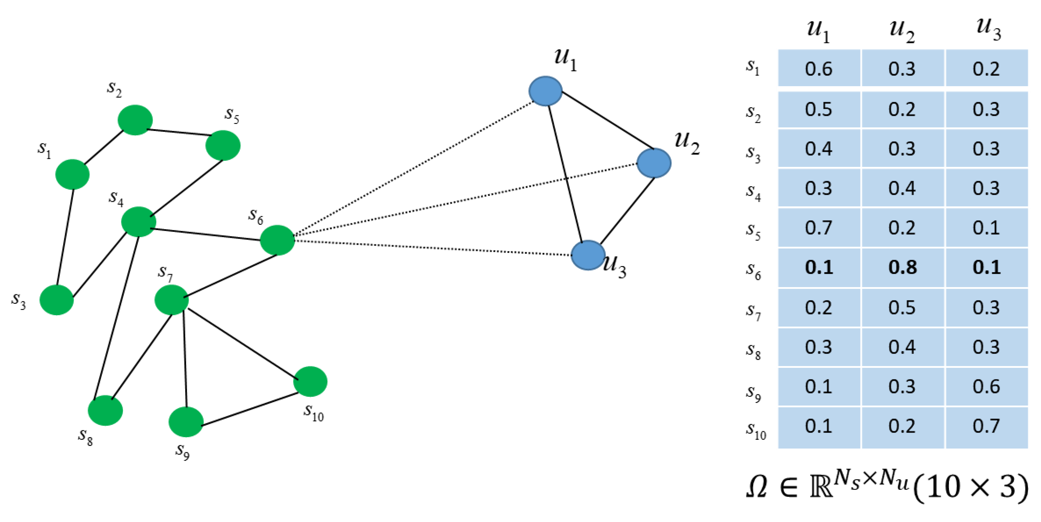
city group graph. We will consider city groups as cities that have strong dependencies, and construct the city group graph as a fully connected graph. We use an undirected graph  g ( v , ε )  to represent the topological structure of a city group graph, as shown in Figure 3, where  v = v 1 , v 2 , , v n  represents the set of all city group nodes, and for any node  v i , we use  R i  to represent its attribute value, and the attribute values of all nodes in  v  can be expressed as the matrix  R ε = ε 1 , ε 2 , , ε n  represents the set of edges of all city groups. For any edge  ε i , we use  M i  to represent its attribute value, and the attribute values of all the edges in  ε  can be expressed as the matrix  M .
Definition 3:
city graph. We use an undirected graph  G ( V , E )  to represent the topology of a city graph, as shown in Figure 3, where  V = v 1 , v 2 , , v n  represents the set of all city nodes, and for any node  V i , we use  X i  to represent its attribute value, and the attribute values of all nodes in  V  can be expressed as the matrix  X E = e 1 , e 2 , , e n  represents the set of all city edges. For any edge  E i , we use  Y i  to represent its attribute value, and the attribute values of all the edges in  E  can be expressed as the matrix  Y . The city graph is constructed as follows:
Y i , j = 1 ( a i a j ) 2 + ( b i b j ) 2 ,
d i , j = ( a i a j ) 2 + ( b i b j ) 2 , 0 < d i , j < r n ,
where  Y i , j  represents the edge attribute of the edge between city  S i  and city  S j ,  [ a i , b i ]  represents the location of city  S i , and  [ a j , b j ]  represents the location of city  S j d i , j  represents the Euclidean distance between city  S i  and city  S j , and  r n  represents the distance threshold. When the distance between the two cities is very large, the cities are hardly affected by each other. The strategy we chose is that when the distance is less than  r n , city  S i  and city  S j  can be connected on the city map.
Definition 4:
urban AQP. This paper mainly predicts the future AQI of a city by giving the historical observation sequence of the city’s location, time, AQI, and weather data. That is, for city  S i , given the city’s location  L , the time vector  T t , and the historical observation sequence  H = ( h i t 1 , h i t 2 , , h i t m )   of m time steps at time t, we can predict the AQI observation sequence  H ^ = ( h ^ i t m + 1 , h ^ i t m + 2 , , h ^ i t m + n )   of the city’s n time steps.

3.2. Framework

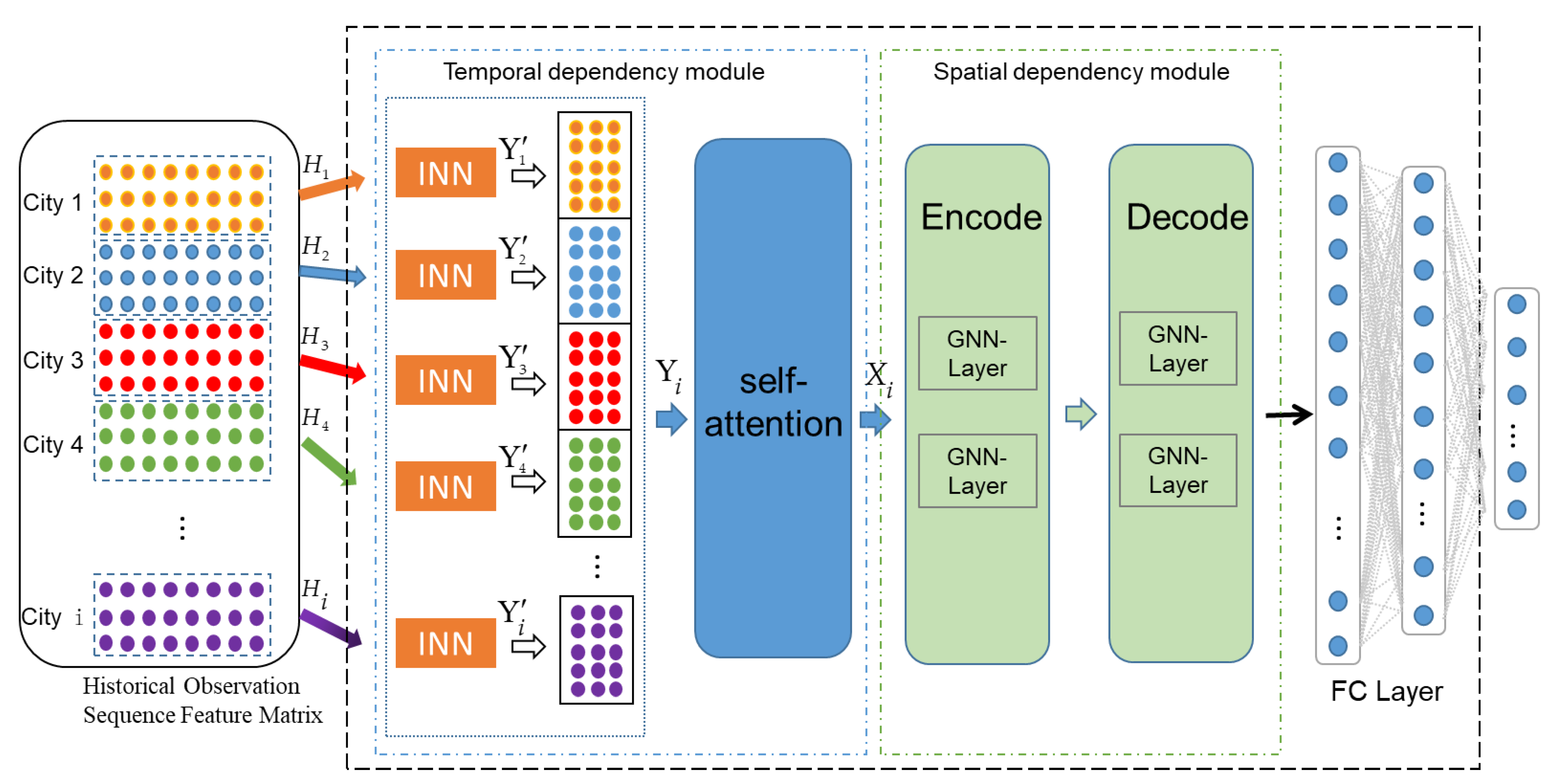
Figure 4 displays the INNGNN framework structure. The temporal dependency module and the spatial dependency module make up the INNGNN. The temporal dependency module extracts the local and global time series features using self-attention and the interpretable trend, and the periodic time series features using INN. The geographical dependence of the geographic location is extracted with the spatial dependency module using GNN. First, the historical observation sequence feature matrix of the 209 cities is input, and the time series features of the different cities are extracted through multiple INNs. Then, the features extracted from the different cities are spliced together. Self-attention is added to the time series in order to capture the local and global dependencies of the various time steps. The input for self-attention is the feature matrix output obtained from splicing several city characteristics that were retrieved using multiple INNs. Natural language processing frequently uses encode–decode to manage mapping relationships and to map one sequence onto another more effectively [59,60]. The GNN module receives its input from the self-attention output. The GNN module uses the encode–decode structure and, to implement the message transmission mechanism, two layers of GNN are layered in the encode–decode, respectively. The decoder uses the output from the encoder to update the city and implement the mapping relationship between the individual cities and city groups. Ultimately, the fully connected layer outputs the prediction findings.

3.3. Temporal Dependency Modeling

3.3.1. Interpretable Neural Networks

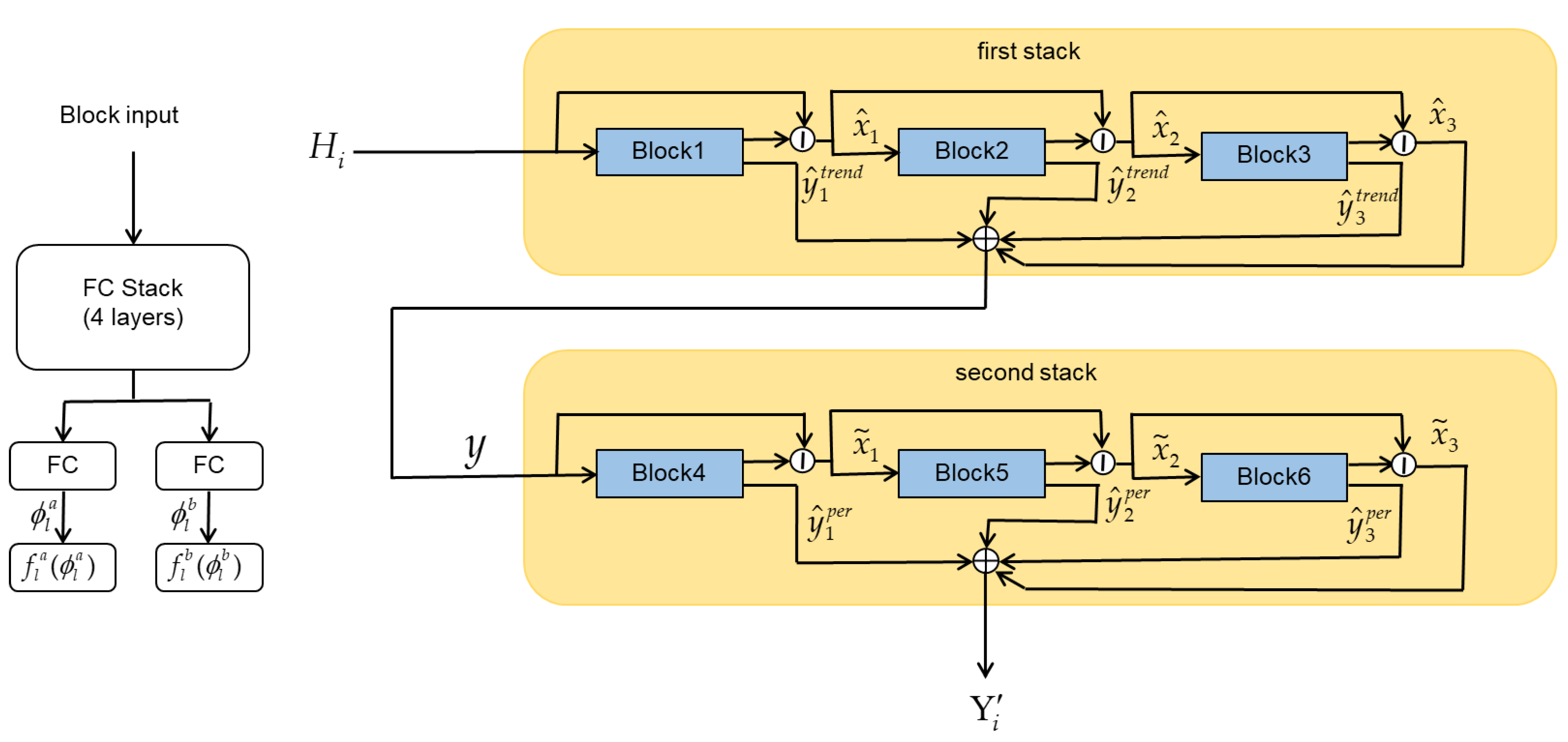
Given its periodic and trend properties, we suggest using interpretable neural networks (INN) to explain the periodicity and trend of the AQI time series. The two stacks comprising the interpretable neural networks, as depicted in Figure 5, are utilized to elucidate the trend and periodicity of the time series. Each stack consists of three blocks, and each block in a stack comprises two parts: the first portion comprises four layers of fully connected layers, and the second component is used to generate the expansion coefficients for the trend and periodic functions. A residual connection is introduced, meaning that each stack completes its own information aggregation procedure, and the input of the current block, less the output of the current block, is used as the input of the next block in order to capture the features of different levels in the input data. Input the historical observation sequence H i of the i-th city, and the first part is described by Formula (3) as follows:
h l , 1 = F C l , 1 ( x l ) , h l , 2 = F C l , 2 ( h l , 1 ) , h l , 3 = F C l , 3 ( h l , 2 ) , h l , 4 = F C l , 4 ( h l , 3 ) ,
where h l , n represents the n th layer of the l th block in each stack, x l represents the residual of the previous block as the input of the current block, and F C represents the standard fully connected layer of the RELU nonlinear function, that is, h l , 1 = R E L U ( W l , 1 H l + b l , 1 ) . The second part is determined using Formula (4), and is described as follows:
ϕ l a = L I N E A R l a ( h l , 4 ) , ϕ l b = L I N E A R l b ( h l , 4 ) y ^ l = f l b ( ϕ l b ) , x ^ l = f l a ( ϕ l a ) ,
where L I N E A R is a simple linear projection layer, such as ϕ l b = W l b h l , 4 . y ^ l and x ^ l represent the output function of the current block of each stack and the residual calculation function of the next block, and ϕ l a and ϕ l b are the expansion coefficients of y ^ l and x ^ l , respectively. The periodicity and trend of the time series’ interpretability are specifically described as follows.
  • Trend: The time series of air quality has a certain trend, as shown in Figure 1b. One of the trend characteristics is that it exhibits an upward or downward trend over time. Either a slowly changing function or a monotone function can simulate the trend. A slowly changing function is used here. The formula is described as follows:
y ^ l t r e n d = T ϕ l b , x ^ l t r e n d = T ϕ l a ,
where T = 1 , t , , t p is a power exponent matrix of t . When the p value is small, such as 3 or 4, it will force y ^ l t r e n d , x ^ l t r e n d to simulate the trend. t is a discrete grid from 0 to N 1 / N , and t is expressed as 0 , 1 , 2 , , N 2 , N 1 T / N , N is the number of steps, the first stack is used as the trend model, the historical sequence H i is used as the input, and the process formulae for the input and output are described as follows:
x ^ 1 = H i x ^ 1 t r e n d , x ^ 2 = x ^ 1 x ^ 2 t r e n d , x ^ 3 = x ^ 2 x ^ 3 t r e n d y = l y ^ l t r e n d + x ^ 3 ,
where x ^ 1 , x ^ 2 , x ^ 3 represent the residuals of each block in the first stack and y represents the final output of the first stack, which is used as the input for the periodicity of the next stack.
  • Periodicity: As seen in Figure 1, there is a certain periodicity to the air quality time series (a). Periodic functions can be chosen to mimic the periodicity. Periodicity is defined as recurring or cyclical patterns within a specific time span. The Fourier series is chosen here, and the formula is described as follows:
y ^ l p e r = P ϕ l b , x ^ l p e r = P ϕ l a ,
where P = [ 1 , cos ( 2 π t ) , , cos ( 2 π N / 2 1 t ) , sin ( 2 π t ) , , sin ( 2 π N / 2 1 t ) ] is the matrix of the sine and cosine waveforms, and the meanings of t and N are the same as those for the trend. The second stack has periodicity characteristics, and the process formulae for the input and output are described as follows:
x ˜ 1 = y x ^ 1 p e r , x ˜ 2 = x ˜ 1 x ^ 2 p e r , x ˜ 3 = x ˜ 2 x ^ 3 p e r Y i = l y ^ l p e r + x ˜ 3 ,
where x ˜ 1 , x ˜ 2 , x ˜ 3 represent the residuals of each block in the second stack, respectively, and Y i represents the final output of the second stack, which is the feature extraction of the i-th city. Then, the features of each city are merged and completed using the stacking approach. The formula is described as follows:
Y i = Y 1 ; Y 2 ; Y 3 ; ; Y 4 ,
where Y i represents the feature merging of all the cities as the input for the next part of the model.

3.3.2. Time Step Local and Global Dependency Capturing

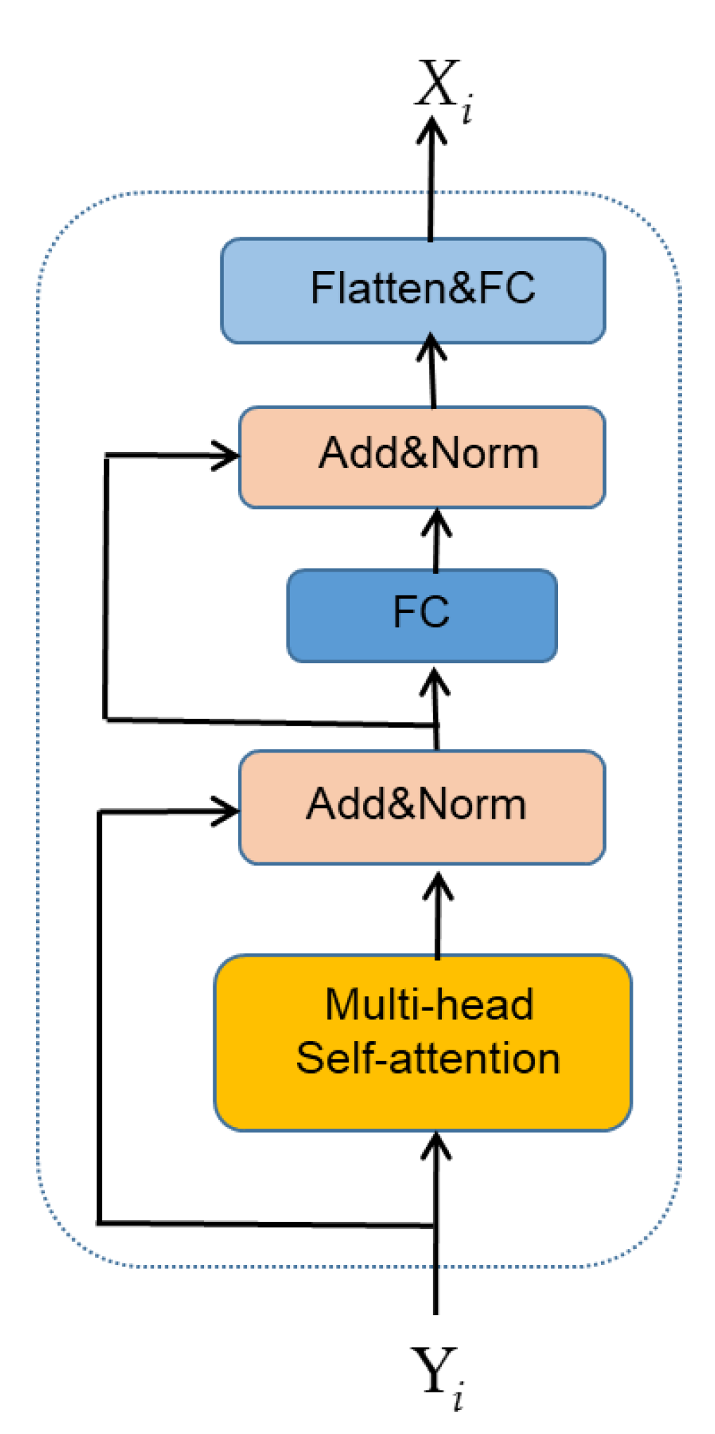
A self-attention method is introduced in order to be able to capture the correlation between the distinct time steps of the time series, as well as the global dependent features and local dependent features. As shown in Figure 6, the self-attention mechanism is designed by referring to transformer [61] architecture, in which a multi-head attention can consider local and global dependencies at the same time. Each head can pay attention to the dependencies between the various time steps by computing the correlation weights between the items. The computation procedure is represented by the following formula:
Q = f ( Y i , W Q ) , K = f ( Y i , W K ) , V = f ( Y i , W V ) ,
A t t e n t i o n ( Q , K , V ) = s o f t max Q K T d K V ,
where Q is the query matrix, K is the key matrix, and V is the value matrix. W Q , W K , W V are all learnable parameters, K T represents the transpose of K , and d K represents the dimension of the K vector. Through matrix multiplication, the degree of association between each element’s query vector and key vector in the matrix is realized, a weight calculation is performed, a normalization operation is realized through s o f t max and, then, a weighted summation is performed. Finally, all the dimensions are flattened using skip connection. The output is obtained through a fully connected (FC) layer.

3.4. Spatial Dependency Modeling

The spatial relationship of the location data for each city can be shown as a graph. The spatial interdependence between cities must be taken into account in order to forecast the air quality of each city. A graph neural network (GNN) is used to construct the dependencies between cities. A detailed description of the composition process is as follows.
  • City grouping: The cities with strong dependencies are assigned to a city group, and each city is mapped onto a city group one by one; this grouping method allows us to identify any potential spatial dependencies between the cities. We use the Ω R N s × N u matrix to represent the mapping relationship between the cities and city groups. Cities can be assigned to multiple city groups. In order to illustrate the correlation between cities and city groups, Ω is randomly initialized during training and optimized at the same time. For the case given, and shown in Figure 7, there are 10 cities divided into 3 city groups, among which the probability of city s 6 being assigned to city group u 1 is 0.1, the probability it of being assigned to city group u 2 is 0.8, and the probability it of being assigned to city group u 3 is 0.1. This shows that city s 6 has a stronger correlation with city group u 2 . In order to capture the spatial dependence between the cities, the geographic location L of the city is added, and the process definition for city grouping is as follows:
X ^ i = F C ( g v ( X i , L i ) ) ,
R j = i = 1 N s Ω j , i T X ^ i ,
where X i is the output of the temporal dependent module, L i represents the geographic coordinates of city s i , X ^ i represents city s i and contains location information, g v ( ) represents the function implemented by using a FC layer, and Ω j ,   i represents city s i assigned to the city probabilities for groups u j . We then have j = 1 N u Ω i , j = 1 , where R j represents the city group representation of the cities assigned to the city group, and Ω T represents the transpose of the matrix Ω .
  • Dependencies between city groups: In a city group, the nodes of each city group are fully connected to generate a fully connected undirected graph g , and the dependency relationship between the city groups is modeled through the mechanism of message passing. The modeling process is as follows:
M i , j = f g ( R i , R j , T t ) ,
M i = { ( R i , R j , M i , j ) } i j M ^ i μ g ( M i ) , R ^ i φ g ( M ^ i , R i ) ,
where M i , j represents the city group u i , the city group u j contains the edge attributes of the time vector T t , and the time vector T t is composed of months, weeks, and days. R i and R j are the attribute values of the city groups u i and u j , respectively, M i is all the information collected and is passed on to city group u i through message passing, and is converted into vector M ^ i after the message passing is completed. R ^ i is the city group representation after the city group u i is updated. f g , μ g , and φ g are all implemented using a FC layer.
  • Dependencies between cities: During city representation, the cities are updated through the process of assigning cities to city groups, and the dependency relationship between the cities is completed through the transmission of messages in city graph G , and the message transmission mechanism is similar to that of the city groups. The difference is that the cities incorporate time series features from the temporal dependency module output, geographic location information, and city group information assigned to the city. The specific process is as follows:
X ˜ i = j = 1 N u Ω i , j R ^ j ,
X i = c o n c a t ( X i , X ˜ i ) ,
Y i = { ( X ˜ i , X ˜ k , Y k , i ) } k k ( i ) Y ^ i μ ( Y i ) , X i φ ( X i , Y ^ i ) ,
where R ^ j represents the updated city group u j ; X ˜ i represents the city group containing city s i ; X i represents city s i and integrates information from the time series features and city group information, which contains geographic location information; and Y i represents all the information collected through message transmissions that were passed to city s i . The neighbor information is aggregated, and is then converted into vector Y ^ i , X i , which is the updated city representation of city s i . The connection functions c o n c a t , μ , and φ are also implemented using a FC layer.

4. Experiments

4.1. Data Description

The INNGNN model was evaluated using the AQI dataset of some cities in China. With an hourly sampling frequency from 1 January 2017 to 30 April 2019, 209 cities were gathered as the dataset. The dataset includes geographic location, weather, and AQI data. The details of the data are as follows:
  • AQI dataset: The data come from the national urban air quality real-time release platform, downloaded from the public platform https://drive.google.com/file/d/1I_vpbLJhOJpNh-TpLdSWsaG3xCpzMVSQ/ (accessed on 15 June 2023.).
  • Weather data: Weather data include the humidity, wind direction, rainfall, wind speed, air pressure, temperature, and visibility. The data come from the open platform for environmental big data http://www.envicloud.cn/ (accessed on 15 June 2023).
  • Geographic location data: The geographic location of each city is shown in Figure 2. The geographic locations of all the cities are marked on the map with red dots.
The time step in this study is 1 h, the time step for a day is 24, and samples with a step of one were generated using a sliding window. We sorted all of the generated samples into training, test, and validation sets, and arranged them chronologically.

4.2. Experimental Settings

Experiments on the GPU were conducted, and all model constructions were completed within the open-source pytorch framework. The training epoch for all the models was set to 300, the batch size was set to 64, and the learning rate was set to 0.001. In addition, the power index p of matrix T was set to 4, the size of the city group was 15, the hidden unit of the GNN was 32, the distance threshold r n was 250 km, and the GNN was set to 2 layers. We used the Adam [62] optimizer to optimize the training of the model.
In addition, AQP is a multiple linear regression problem. In order to effectively evaluate the model, the deviation between the predicted value and the observed value was calculated, using the mean absolute error (MAE) and the root mean square error (RMSE) as the indicators for the model’s evaluation. The calculation process is as follows:
M A E = 1 N S × τ i = 1 N S t = 1 τ O i t O ˜ i t ,
R M S E = 1 N S × τ i = 1 N S t = 1 τ O i t O ˜ i t 2 ,
where τ represents the number of time samples, and O i j and O ˜ i j represent the observed value and predicted value for city i at time t , respectively. The same experimental parameters were used for five verifications for each of our tests, and the average result was used to determine the final outcome.

4.3. Experimental Results

4.3.1. Comparative Prediction Results

In this section, the INNGNN model is compared to the following baseline models:
DeeperGCN [63]: An extended form of GCN, DeeperGCN uses a deeper network structure that enhances its capacity to model complicated graph data. Eight layers were used in the experimental comparison.
LSTM [35]: LSTM (long short-term memory) is a variant of a recurrent neural network (RNN), which solves the problems of traditional RNNs regarding gradient disappearance and gradient explosion. The experiment’s hidden unit was set to 32, the predicted value of the AQI was the output, and the features from the historical observation sequence were the input.
GC-LSTM [11]: The GC-LSTM model combines a graph convolutional neural network (GCN) with a long short-term memory network (LSTM). In the experimental settings, the optimal setting of LSTM hidden units was 64.
GAGNN [10]: GAGNN is a neural network model designed to analyze graph data with intra- and inter-group links. It is specifically designed for graph-structured data. The hidden layer unit was set to 32 in the experiment.
SHARE [64]: With numerous hierarchical recursive layers and graph attention layers, SHARE is a semi-supervised hierarchical recursive graph neural network model for graph-structured data. The shared semi-supervised portion of the experimental settings was removed, while the other parameters stayed the same.
ST-UNet [65]: ST-UNet is a neural network model for processing graph-structured time series data. To improve the time series modeling ability of the graph-structured time series data, the model presented an the extended GRU. The hidden unit of the expanded GRU wad 32 in the experiment.
XGBoost [66]: XGBoost is based on the decision tree model and introduces feature parallel computing. For parameter optimization of the experiments, network search methods were used.
HighAir [67]: A neural network model, HighAir uses graph structural information to optimize the graphs. It creates connections between the graph data by simulating the dynamic elements and creating the graphs from a hierarchical viewpoint.
The prediction task results for the baseline model and the INNGNN model, which were run on the dataset for one to six hours per day, are displayed in Table 1. The INNGNN model’s assessment metrics, MAE and RMSE, showed the best prediction results across all the prediction ranges, demonstrating the model’s efficacy in the task of spatiotemporal air quality prediction.
In terms of performance, the hybrid INNGNN model is still superior to the graph neural network. As shown in Table 1, for the 1 h and 6 h prediction tasks, the MAE error of the INNGNN model was reduced by 19% and 10%, respectively, and the RMSE error was reduced by 27% and 7%, compared to the DeeperGCN model. In the 6 h prediction task, the RMSE error of the INNGNN model was reduced by 4% and 5.8%, compared to the SHARE model and the ST-UNet model, respectively. When compared to the enhanced graph neural network models, GAGNN and HighAir, the INNGNN model improved the MAE and RMSE errors for short-term, medium-term, and long-term predictions during the 1 h to 6 h prediction tasks. For the 1 h prediction task, the MAE error was reduced by 6.6% and 8.6%, respectively. Our model’s MAE and RMSE errors are still significantly better than those of the HighAir model, which has a better prediction effect. From this thorough comparison, the INNGNN model improves upon the graph neural network foundation by incorporating the extraction of temporal data. This allows for a more accurate capture of the temporal and spatial connections, particularly for long-term predictions, demonstrating its superior benefits.
Regarding the time series feature extraction process, the INNGNN model adds trend and periodic feature extraction, as compared to the GC-LSTM hybrid model. This greatly enhances the feature capture of burst points. In order to better extract the spatiotemporal aspects of air quality prediction, the feature extraction for the correlation between cities is integrated into the spatial feature extraction process concurrently. As demonstrated in Table 1, the INNGNN model’s prediction accuracy outperformed that of the GC-LSTM model over the 1–6 h prediction test.

4.3.2. Comparative Analysis: Individual Module vs. Hybrid Model

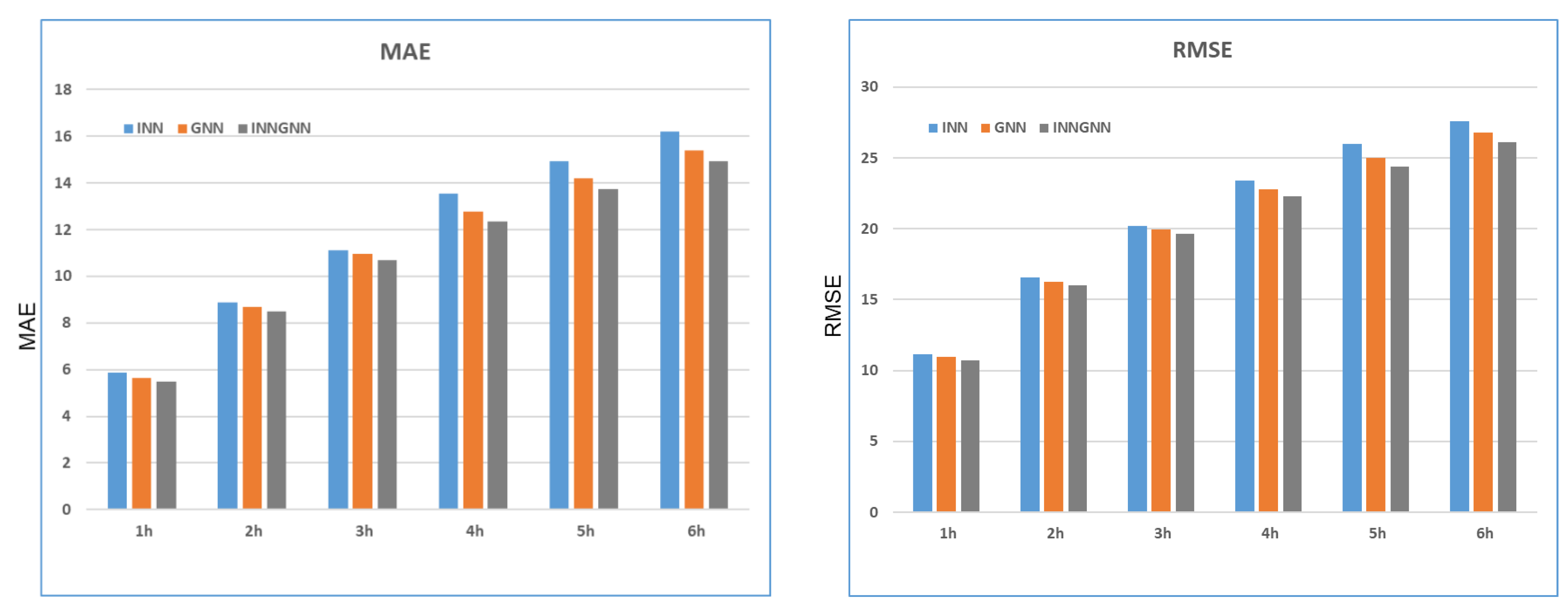
A few of the model’s modules were investigated to confirm that the suggested hybrid INNGNN model is accurate in its forecasting performance. Figure 8 illustrates how we compared the RMSE and MAE values of the prediction outcomes of the GNN module, INNGNN model, and INN module from one hour to six hours, without including self-attention. The results displayed in the figure demonstrate the greater predictive performance of the hybrid model, with the INNGNN model outperforming each separate module.

4.3.3. Ablation Studies

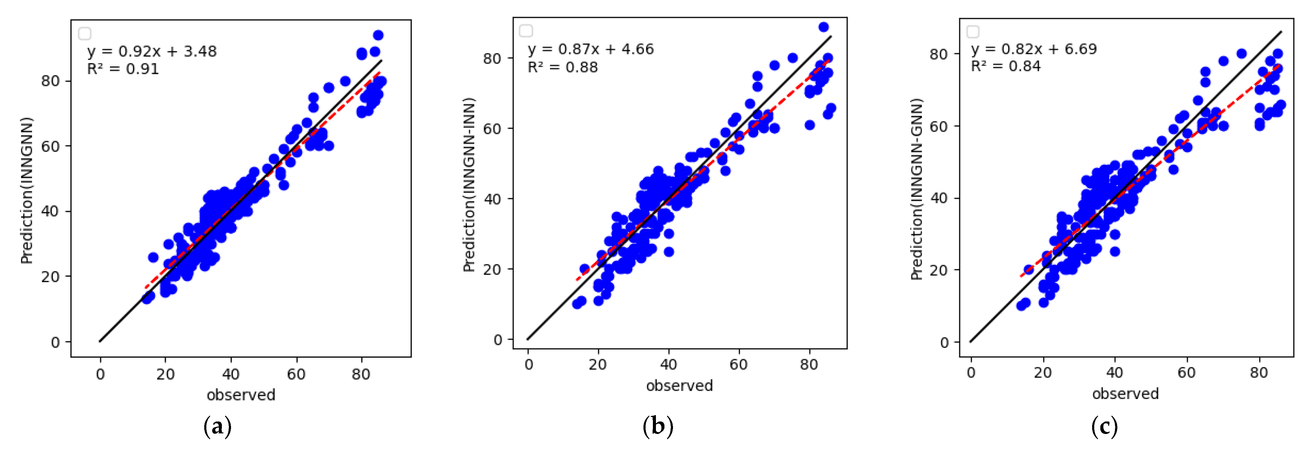
Ablation investigations were carried out to confirm the prediction performance of our proposed INNGNN model. The model for prediction used in the experiment was renamed INNGNN-INN after the INN part was removed, and INNGNN-GNN after the GNN part was removed for making predictions. This model compares the linear correlation between the INNGNN model and its corresponding predicted values. Among these three models, it can be observed from Figure 9 that the INNGNN model has the best fitting effect on the predicted value and the observed value, and the correlation coefficient R 2 is 0.91, which is higher than that of the INNGNN-INN model (the correlation coefficient R 2 is 0.88), indicating that the temporal correlation results in a significant improvement of the prediction results. At the same time, it is higher than the INNGNN-GNN model (the correlation coefficient R 2 is 0.88), indicating that the spatial correlation significantly improved the prediction results.

4.3.4. Display and Analysis

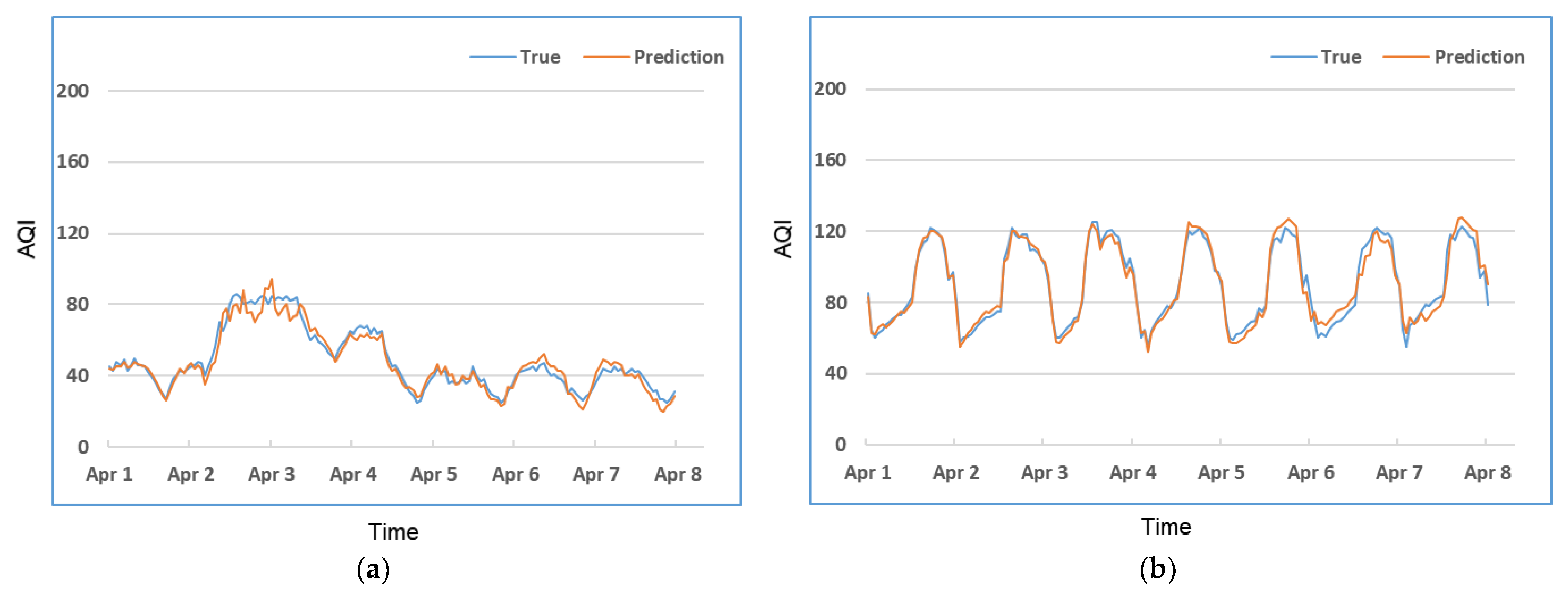
This section shows the AQP results for two cities from 1 April to 8 April using the INNGNN model. In Figure 10, the blue line represents the real value, and the red line represents the predicted value. Figure 10a represents the prediction effect for cities with low-scale fluctuations in air quality, and Figure 10b represents the prediction effect for cities with high-scale fluctuations in air quality. Our INNGNN model reacted promptly to time series fluctuations in both scenarios. The AQI increased significantly between 2 April and 3 April, as shown in Figure 10a, but the INNGNN model was still able to react promptly to the time series changes, demonstrating the model’s strong accuracy and efficient performance.

5. Conclusions

This study proposes a hybrid model, INNGNN, to forecast air quality by combining GNN and self-attention. The INN module is used to fully extract the time series characteristics in order to obtain the temporal dependence, and to give the periodicity and trend the interpretability needed for forecasting. These issues with periodicity and trend are often ignored in time series forecasting. Furthermore, the self-attention mechanism is incorporated in order to capture the time series’ local and global dependencies, as well as the varying relevance of each input feature at different times. In order to achieve the expected spatial dependencies, the combination of GNN models can determine the connection relationship between cities in order to capture the dependencies between them. When the INNGNN model was compared to previous models and assessed using real air quality datasets, it performed better over a range of prediction ranges. To further validate its performance, ablation experiments were conducted by comparing different modules of the model, and the INNGNN consistently exhibited superior performance.
In conclusion, the spatiotemporal aspects of urban air quality data are effectively captured by the INNGNN model, and this model can be expanded and used for other multivariate timeseries spatiotemporal applications. Environmental factors or specific dataset characteristics that were not considered in this study may influence the model’s performance. Additionally, the possibility of further investigating and improving the comprehensibility of the model’s forecasts exists. In subsequent studies, we want to investigate further how graph neural networks could be integrated with other time series models in order to increase the predictability and versatility of these models. We will also concentrate on enhancing the interpretability of the model and resolving any biases or limitations present in the dataset.

Author Contributions

Conceptualization, H.D. and G.N.; methodology, H.D. and G.N.; software, H.D. and G.N.; validation, H.D. and G.N.; formal analysis, H.D. and G.N.; investigation, H.D. and G.N.; resources, H.D. and G.N.; data curation, H.D. and G.N.; writing—original draft preparation, H.D. and G.N.; writing—review and editing, H.D. and G.N.; visualization, H.D. and G.N.; supervision, H.D. and G.N. All authors have read and agreed to the published version of the manuscript.

Funding

This research received no external funding.

Institutional Review Board Statement

Not applicable.

Informed Consent Statement

Not applicable.

Data Availability Statement

The data presented in this study are openly available in https://drive.google.com/file/d/1I_vpbLJhOJpNh-TpLdSWsaG3xCpzMVSQ/. The flared volume data are available from 1 January 2017 to 30 April 2019 (data http://www.envicloud.cn/ (accessed on 15 June 2023)).

Conflicts of Interest

The authors declare no conflict of interest.

References

  1. Lin, Y.-C.; Chi, W.-J.; Lin, Y.-Q. The Improvement of Spatial-Temporal Resolution of PM2.5 Estimation Based on Micro-Air Quality Sensors by Using Data Fusion Technique. Environ. Int. 2020, 134, 105305. [Google Scholar] [CrossRef] [PubMed]
  2. Wijnands, J.S.; Nice, K.A.; Seneviratne, S.; Thompson, J.; Stevenson, M. The Impact of the COVID-19 Pandemic on Air Pollution: A Global Assessment Using Machine Learning Techniques. Atmos. Pollut. Res. 2022, 13, 101438. [Google Scholar] [CrossRef] [PubMed]
  3. Brett, G.J.; Whitt, D.B.; Long, M.C.; Bryan, F.O.; Feloy, K.; Richards, K.J. Submesoscale Effects on Changes to Export Production Under Global Warming. Glob. Biogeochem. Cycles 2023, 37, e2022GB007619. [Google Scholar] [CrossRef]
  4. Pruthi, D.; Liu, Y. Low-Cost Nature-Inspired Deep Learning System for PM2.5 Forecast over Delhi, India. Environ. Int. 2022, 166, 107373. [Google Scholar] [CrossRef] [PubMed]
  5. Balachandran, S.; Chang, H.H.; Pachon, J.E.; Holmes, H.A.; Mulholland, J.A.; Russell, A.G. Bayesian-Based Ensemble Source Apportionment of PM2.5. Environ. Sci. Technol. 2013, 47, 13511–13518. [Google Scholar] [CrossRef] [PubMed]
  6. Singh, K.P.; Gupta, S.; Kumar, A.; Shukla, S.P. Linear and Nonlinear Modeling Approaches for Urban Air Quality Prediction. Sci. Total Environ. 2012, 426, 244–255. [Google Scholar] [CrossRef] [PubMed]
  7. Navares, R.; Aznarte, J.L. Predicting Air Quality with Deep Learning LSTM: Towards Comprehensive Models. Ecol. Inform. 2020, 55, 101019. [Google Scholar] [CrossRef]
  8. Zhang, C.; Yan, J.; Li, C.; Rui, X.; Liu, L.; Bie, R. On Estimating Air Pollution from Photos Using Convolutional Neural Network. In Proceedings of the 24th ACM International Conference on Multimedia; Association for Computing Machinery, New York, NY, USA, 15–19 October 2016; Springer: Berlin/Heidelberg, Germany, 2016; pp. 297–301. [Google Scholar]
  9. Bruna, J.; Zaremba, W.; Szlam, A.; LeCun, Y. Spectral Networks and Locally Connected Networks on Graphs 2014. arXiv 2014, arXiv:1312.6203. [Google Scholar]
  10. Chen, L.; Xu, J.; Wu, B.; Qian, Y.; Du, Z.; Li, Y.; Zhang, Y. Group-Aware Graph Neural Network for Nationwide City Air Quality Forecasting 2021. arXiv 2021, arXiv:2108.12238. [Google Scholar]
  11. Qi, Y.; Li, Q.; Karimian, H.; Liu, D. A Hybrid Model for Spatiotemporal Forecasting of PM2.5 Based on Graph Convolutional Neural Network and Long Short-Term Memory. Sci. Total Environ. 2019, 664, 1–10. [Google Scholar] [CrossRef]
  12. Baek, J.; Lee, C.; Yu, H.; Baek, S.; Lee, S.; Lee, S.; Park, C. Automatic Sleep Scoring Using Intrinsic Mode Based on Interpretable Deep Neural Networks. IEEE Access 2022, 10, 36895–36906. [Google Scholar] [CrossRef]
  13. Oreshkin, B.N.; Carpov, D.; Chapados, N.; Bengio, Y. N-BEATS: Neural Basis Expansion Analysis for Interpretable Time Series Forecasting 2020. arXiv 2020, arXiv:1905.10437. [Google Scholar]
  14. Huang, D.; Tang, S.; Zhou, D.; Hao, J. Nox Emission Estimation in Gas Turbines via Interpretable Neural Network Observer with Adjustable Intermediate Layer Considering Ambient and Boundary Conditions. Measurement 2022, 189, 110429. [Google Scholar] [CrossRef]
  15. Byun, D.W.; Ching, J.K.S. Science Algorithms OF THE Epa Models-3 Community Multiscale Air Quality (CMAQ) Modeling System; Office of Research and Development, US Environmental Protection Agency: Washington, DC, USA, 1999. [Google Scholar]
  16. Byun, D.; Schere, K.L. Review of the Governing Equations, Computational Algorithms, and Other Components of the Models-3 Community Multiscale Air Quality (CMAQ) Modeling System. Appl. Mech. Rev. 2006, 59, 51–77. [Google Scholar] [CrossRef]
  17. Mueller, S.F.; Mallard, J.W. Contributions of Natural Emissions to Ozone and PM2.5 as Simulated by the Community Multiscale Air Quality (CMAQ) Model. Available online: https://pubs.acs.org/doi/pdf/10.1021/es103645m (accessed on 25 June 2023).
  18. Environ. User’s Guide to the Comprehensive Air Quality Model with Extensions (CAMx) 2014. Available online: http://www.camx.com (accessed on 11 July 2023).
  19. Koo, Y.-S.; Choi, D.-R.; Kwon, H.-Y.; Jang, Y.-K.; Han, J.-S. Improvement of PM10 Prediction in East Asia Using Inverse Modeling. Atmos. Environ. 2015, 106, 318–328. [Google Scholar] [CrossRef]
  20. Ni, X.Y.; Huang, H.; Du, W.P. Relevance Analysis and Short-Term Prediction of PM2.5 Concentrations in Beijing Based on Multi-Source Data. Atmos. Environ. 2017, 150, 146–161. [Google Scholar] [CrossRef]
  21. Zhang, L.; Lin, J.; Qiu, R.; Hu, X.; Zhang, H.; Chen, Q.; Tan, H.; Lin, D.; Wang, J. Trend Analysis and Forecast of PM2.5 in Fuzhou, China Using the ARIMA Model. Ecol. Indic. 2018, 95, 702–710. [Google Scholar] [CrossRef]
  22. García Nieto, P.J.; Sánchez Lasheras, F.; García-Gonzalo, E.; de Cos Juez, F.J. PM10 Concentration Forecasting in the Metropolitan Area of Oviedo (Northern Spain) Using Models Based on SVM, MLP, VARMA and ARIMA: A Case Study. Sci. Total Environ. 2018, 621, 753–761. [Google Scholar] [CrossRef]
  23. Ma, Z.; Hu, X.; Huang, L.; Bi, J.; Liu, Y. Estimating Ground-Level PM2.5 in China Using Satellite Remote Sensing. Environ. Sci. Technol. 2014, 48, 7436–7444. [Google Scholar] [CrossRef]
  24. Masmoudi, S.; Elghazel, H.; Taieb, D.; Yazar, O.; Kallel, A. A Machine-Learning Framework for Predicting Multiple Air Pollutants’ Concentrations via Multi-Target Regression and Feature Selection. Sci. Total Environ. 2020, 715, 136991. [Google Scholar] [CrossRef]
  25. Leong, W.C.; Kelani, R.O.; Ahmad, Z. Prediction of Air Pollution Index (API) Using Support Vector Machine (SVM). J. Environ. Chem. Eng. 2020, 8, 103208. [Google Scholar] [CrossRef]
  26. Zhou, Y.; Chang, F.-J.; Chang, L.-C.; Kao, I.-F.; Wang, Y.-S.; Kang, C.-C. Multi-Output Support Vector Machine for Regional Multi-Step-Ahead PM2.5 Forecasting. Sci. Total Environ. 2019, 651, 230–240. [Google Scholar] [CrossRef] [PubMed]
  27. He, H.; Li, M.; Wang, W.; Wang, Z.; Xue, Y. Prediction of PM2.5 Concentration Based on the Similarity in Air Quality Monitoring Network. Build. Environ. 2018, 137, 11–17. [Google Scholar] [CrossRef]
  28. Li, Z.; Yang, J. PM-25 Forecasting Use Reconstruct Phase Space LS-SVM. In Proceedings of the 2010 The 2nd Conference on Environmental Science and Information Application Technology, Wuhan, China, 17–18 July 2010; Volume 1, pp. 143–146. [Google Scholar]
  29. Beckerman, B.S.; Jerrett, M.; Martin, R.V.; van Donkelaar, A.; Ross, Z.; Burnett, R.T. Application of the Deletion/Substitution/Addition Algorithm to Selecting Land Use Regression Models for Interpolating Air Pollution Measurements in California. Atmos. Environ. 2013, 77, 172–177. [Google Scholar] [CrossRef]
  30. He, Z.; Liu, P.; Zhao, X.; He, X.; Liu, J.; Mu, Y. Responses of Surface O3 and PM2.5 Trends to Changes of Anthropogenic Emissions in Summer over Beijing during 2014–2019: A Study Based on Multiple Linear Regression and WRF-Chem. Sci. Total Environ. 2022, 807, 150792. [Google Scholar] [CrossRef] [PubMed]
  31. Wahid, H.; Ha, Q.P.; Duc, H.N. Computational Intelligence Estimation of Natural Background Ozone Level and Its Distribution for Air Quality Modelling and Emission Control. In Proceedings of the 28th International Symposium on Automation and Robotics in Construction (ISARC 2011), Seoul, Republic of Korea, 29 June–2 July 2011. [Google Scholar]
  32. Antanasijević, D.Z.; Pocajt, V.V.; Povrenović, D.S.; Ristić, M.Đ.; Perić-Grujić, A.A. PM10 Emission Forecasting Using Artificial Neural Networks and Genetic Algorithm Input Variable Optimization. Sci. Total Environ. 2013, 443, 511–519. [Google Scholar] [CrossRef] [PubMed]
  33. Kamal, M.M.; Jailani, R.; Shauri, R.L.A. Prediction of Ambient Air Quality Based on Neural Network Technique. In Proceedings of the 2006 4th Student Conference on Research and Development, Shah Alam, Malaysia, 27–28 June 2006; pp. 115–119. [Google Scholar]
  34. Loy-Benitez, J.; Vilela, P.; Li, Q.; Yoo, C. Sequential Prediction of Quantitative Health Risk Assessment for the Fine Particulate Matter in an Underground Facility Using Deep Recurrent Neural Networks. Ecotoxicol. Environ. Saf. 2019, 169, 316–324. [Google Scholar] [CrossRef] [PubMed]
  35. Lu, X.; Sha, Y.H.; Li, Z.; Huang, Y.; Chen, W.; Chen, D.; Shen, J.; Chen, Y.; Fung, J.C.H. Development and Application of a Hybrid Long-Short Term Memory—Three Dimensional Variational Technique for the Improvement of PM2.5 Forecasting. Sci. Total Environ. 2021, 770, 144221. [Google Scholar] [CrossRef]
  36. Ulpiani, G.; Duhirwe, P.N.; Yun, G.Y.; Lipson, M.J. Meteorological Influence on Forecasting Urban Pollutants: Long-Term Predictability versus Extreme Events in a Spatially Heterogeneous Urban Ecosystem. Sci. Total Environ. 2022, 814, 152537. [Google Scholar] [CrossRef]
  37. Wu, C.; He, H.; Song, R.; Peng, Z. Prediction of Air Pollutants on Roadside of the Elevated Roads with Combination of Pollutants Periodicity and Deep Learning Method. Build. Environ. 2022, 207, 108436. [Google Scholar] [CrossRef]
  38. Huang, G.; Li, X.; Zhang, B.; Ren, J. PM2.5 Concentration Forecasting at Surface Monitoring Sites Using GRU Neural Network Based on Empirical Mode Decomposition. Sci. Total Environ. 2021, 768, 144516. [Google Scholar] [CrossRef]
  39. Xu, R.; Deng, X.; Wan, H.; Cai, Y.; Pan, X. A Deep Learning Method to Repair Atmospheric Environmental Quality Data Based on Gaussian Diffusion. J. Clean. Prod. 2021, 308, 127446. [Google Scholar] [CrossRef]
  40. Zhang, B.; Zou, G.; Qin, D.; Lu, Y.; Jin, Y.; Wang, H. A Novel Encoder-Decoder Model Based on Read-First LSTM for Air Pollutant Prediction. Sci. Total Environ. 2021, 765, 144507. [Google Scholar] [CrossRef] [PubMed]
  41. Fang, W.; Zhu, R.; Lin, J.C.-W. An Air Quality Prediction Model Based on Improved Vanilla LSTM with Multichannel Input and Multiroute Output. Expert Syst. Appl. 2023, 211, 118422. [Google Scholar] [CrossRef]
  42. Zhang, B.; Zhang, H.; Zhao, G.; Lian, J. Constructing a PM2.5 Concentration Prediction Model by Combining Auto-Encoder with Bi-LSTM Neural Networks. Environ. Model. Softw. 2019, 124, 104600. [Google Scholar] [CrossRef]
  43. Eren, B.; Aksangür, İ.; Erden, C. Predicting next Hour Fine Particulate Matter (PM2.5) in the Istanbul Metropolitan City Using Deep Learning Algorithms with Time Windowing Strategy. Urban Clim. 2023, 48, 101418. [Google Scholar] [CrossRef]
  44. Zhu, J.; Deng, F.; Zhao, J.; Zheng, H. Attention-Based Parallel Networks (APNet) for PM2.5 Spatiotemporal Prediction—ScienceDirect. Sci. Total Environ. 2021, 769, 145082. [Google Scholar] [CrossRef]
  45. Rijal, N.; Gutta, R.T.; Cao, T.; Lin, J.; Bo, Q.; Zhang, J. Ensemble of Deep Neural Networks for Estimating Particulate Matter from Images. In Proceedings of the 2018 IEEE 3rd International Conference on Image, Vision and Computing (ICIVC), Chongqing, China, 27–29 June 2018; pp. 733–738. [Google Scholar]
  46. Pak, U.; Ma, J.; Ryu, U.; Ryom, K.; Juhyok, U.; Pak, K.; Pak, C. Deep Learning-Based PM2.5 Prediction Considering the Spatiotemporal Correlations: A Case Study of Beijing, China. Sci. Total Environ. 2020, 699, 133561. [Google Scholar] [CrossRef]
  47. Yan, R.; Liao, J.; Yang, J.; Sun, W.; Nong, M.; Li, F. Multi-Hour and Multi-Site Air Quality Index Forecasting in Beijing Using CNN, LSTM, CNN-LSTM, and Spatiotemporal Clustering. Expert Syst. Appl. 2021, 169, 114513. [Google Scholar] [CrossRef]
  48. Zhang, B.; Geng, Z.; Zhang, H.; Pan, J. Densely Connected Convolutional Networks with Attention Long Short-Term Memory for Estimating PM2.5 Values from Images. J. Clean. Prod. 2022, 333, 130101. [Google Scholar] [CrossRef]
  49. Wen, C.; Liu, S.; Yao, X.; Peng, L.; Li, X.; Hu, Y.; Chi, T. A Novel Spatiotemporal Convolutional Long Short-Term Neural Network for Air Pollution Prediction. Sci. Total Environ. 2019, 654, 1091–1099. [Google Scholar] [CrossRef] [PubMed]
  50. Zhu, M.; Xie, J. Investigation of Nearby Monitoring Station for Hourly PM2.5 Forecasting Using Parallel Multi-Input 1D-CNN-biLSTM. Expert Syst. Appl. 2023, 211, 118707. [Google Scholar] [CrossRef]
  51. Gilik, A.; Ogrenci, A.S.; Ozmen, A. Air Quality Prediction Using CNN+LSTM-Based Hybrid Deep Learning Architecture. Environ. Sci. Pollut. Res. 2022, 29, 11920–11938. [Google Scholar] [CrossRef] [PubMed]
  52. Wu, C.; He, H.; Song, R.; Zhu, X.; Peng, Z.; Fu, Q.; Pan, J. A Hybrid Deep Learning Model for Regional O3 and NO2 Concentrations Prediction Based on Spatiotemporal Dependencies in Air Quality Monitoring Network. Environ. Pollut. 2023, 320, 121075. [Google Scholar] [CrossRef] [PubMed]
  53. Liu, B.; Wang, M.; Guesgen, H.W. A Hybrid Model for Spatial–Temporal Prediction of PM2.5 Based on a Time Division Method. Int. J. Environ. Sci. Technol. 2023, 20, 12195–12206. [Google Scholar] [CrossRef]
  54. Kow, P.-Y.; Chang, L.-C.; Lin, C.-Y.; Chou, C.C.-K.; Chang, F.-J. Deep Neural Networks for Spatiotemporal PM2.5 Forecasts Based on Atmospheric Chemical Transport Model Output and Monitoring Data. Environ. Pollut. 2022, 306, 119348. [Google Scholar] [CrossRef] [PubMed]
  55. Zhang, K.; Yang, X.; Cao, H.; Thé, J.; Tan, Z.; Yu, H. Multi-Step Forecast of PM2.5 and PM10 Concentrations Using Convolutional Neural Network Integrated with Spatial–Temporal Attention and Residual Learning. Environ. Int. 2023, 171, 107691. [Google Scholar] [CrossRef]
  56. Zeng, Y.; Chen, J.; Jin, N.; Jin, X.; Du, Y. Air Quality Forecasting with Hybrid LSTM and Extended Stationary Wavelet Transform. Build. Environ. 2022, 213, 108822. [Google Scholar] [CrossRef]
  57. Choudhury, A.; Middya, A.I.; Roy, S. Attention Enhanced Hybrid Model for Spatiotemporal Short-Term Forecasting of Particulate Matter Concentrations. Sustain. Cities Soc. 2022, 86, 104112. [Google Scholar] [CrossRef]
  58. Wang, X.; Wang, Y.; Peng, J.; Zhang, Z.; Tang, X. A Hybrid Framework for Multivariate Long-Sequence Time Series Forecasting. Appl. Intell. 2023, 53, 13549–13568. [Google Scholar] [CrossRef]
  59. Cui, Z.; Zhang, J.; Noh, G.; Park, H.J. MFDGCN: Multi-Stage Spatio-Temporal Fusion Diffusion Graph Convolutional Network for Traffic Prediction. Appl. Sci. 2022, 12, 2688. [Google Scholar] [CrossRef]
  60. Song, C.; Lin, Y.; Guo, S.; Wan, H. Spatial-Temporal Synchronous Graph Convolutional Networks: A New Framework for Spatial-Temporal Network Data Forecasting. Proc. AAAI Conf. Artif. Intell. 2020, 34, 914–921. [Google Scholar] [CrossRef]
  61. Vaswani, A.; Shazeer, N.; Parmar, N.; Uszkoreit, J.; Jones, L.; Gomez, A.N.; Kaiser, L.; Polosukhin, I. Attention Is All You Need 2023. arXiv 2023, arXiv:1706.03762. [Google Scholar]
  62. Kingma, D.P.; Ba, J. Adam: A Method for Stochastic Optimization 2017. arXiv 2017, arXiv:1412.6980. [Google Scholar]
  63. Li, G.; Xiong, C.; Thabet, A.; Ghanem, B. DeeperGCN: All You Need to Train Deeper GCNs. arXiv 2020, arXiv:2006.07739. [Google Scholar] [CrossRef]
  64. Zhang, W.; Liu, H.; Liu, Y.; Zhou, J.; Xiong, H. Semi-Supervised Hierarchical Recurrent Graph Neural Network for City-Wide Parking Availability Prediction. In Proceedings of the National Conference on Artificial Intelligence, New York, NY, USA, 7–12 February 2020. [Google Scholar]
  65. Yu, B.; Yin, H.; Zhu, Z. ST-UNet: A Spatio-Temporal U-Network for Graph-Structured Time Series Modeling 2021. arXiv 2021, arXiv:1903.05631. [Google Scholar]
  66. Chen, T.; Guestrin, C. XGBoost: A Scalable Tree Boosting System. In Proceedings of the 22nd ACM SIGKDD International Conference on Knowledge Discovery and Data Mining, San Francisco, CA, USA, 13–17 August 2016; pp. 785–794. [Google Scholar]
  67. Xu, J.; Chen, L.; Lv, M.; Zhan, C.; Chen, S.; Chang, J. HighAir: A Hierarchical Graph Neural Network-Based Air Quality Forecasting Method. arXiv 2021, arXiv:2101.04264. [Google Scholar]
  68. Hsu, A.; Reuben, A.; Shindell, D.; De Sherbinin, A.; Levy, M. Toward the next Generation of Air Quality Monitoring Indicators. Atmos. Environ. 2013, 80, 561–570. [Google Scholar] [CrossRef]
Figure 1. (a) Periodicity: air quality changes periodically over a week. (b) Trend: air quality has a tendency to change over a day. The horizontal axis represents time, and the vertical axis represents AQI value.
Atmosphere 14 01807 g001
Figure 2. Geographical location of 209 cities.
Atmosphere 14 01807 g002
Figure 3. City graph and city group graph.
Atmosphere 14 01807 g003
Figure 4. INNGNN framework.
Atmosphere 14 01807 g004
Figure 5. Architecture of interpretable neural networks (INN). Atmosphere 14 01807 i001: represents the input minus the output of each block; : represents the addition of the output information from each block in every stack with the residual information from the final block, for information aggregation.
Atmosphere 14 01807 g005
Figure 6. Self-attention network mechanism.
Atmosphere 14 01807 g006
Figure 7. Relationship between cities and city groups.
Atmosphere 14 01807 g007
Figure 8. Comparison of MAE value and RMSE value of prediction results of the INN module, GNN module, and INNGNN model.
Atmosphere 14 01807 g008
Figure 9. Correlations between observations and predictions on the test dataset for different components of the model: (a) INNGNN model; (b) INNGNN-INN model; and (c) INNGNN-GNN model. The red dashed line and black solid line are the regression lines, and y = x is the reference line, respectively.
Atmosphere 14 01807 g009
Figure 10. Final predictions for city 1 and city 2: (a) city 1 is a city with low-scale fluctuations, and (b) city 2 is a city with high-scale fluctuations. The AQI value was calculated by mapping the concentration values of different pollutants onto indices, calculating the sub-index of each pollutant, and taking the highest value as the AQI value [68].
Atmosphere 14 01807 g010
Table 1. Prediction results of the INNGNN model and baseline model.
ModelMetric1 h2 h3 h4 h5 h6 h
INNGNNMAE5.488.4910.6712.3413.7214.91
RMSE10.7016.0319.6622.2924.3726.11
DeeperGCNMAE6.549.7411.7713.4015.2916.41
RMSE13.6718.9321.1423.8326.2528.02
LSTMMAE6.5010.2613.1815.5217.4018.91
RMSE13.8519.2623.5226.8329.4631.55
GC-LSTMMAE5.959.1611.5813.4615.0016.31
RMSE11.9116.9820.8223.6925.9727.82
GAGNNMAE5.568.5910.8012.5213.9115.10
RMSE10.8116.1719.8422.5124.6326.37
SHAREMAE5.849.0711.4913.3514.7415.79
RMSE11.2716.8420.7723.6025.8027.38
ST-UNetMAE5.959.3011.5813.3814.8216.02
RMSE11.7418.0121.3423.9025.9427.64
XGBoostMAE6.8510.8913.9916.2718.1419.56
RMSE14.2519.8024.7228.1430.6333.44
HighAirMAE5.508.5210.8112.5014.0015.09
RMSE10.8016.1019.8522.7024.9126.40
Disclaimer/Publisher’s Note: The statements, opinions and data contained in all publications are solely those of the individual author(s) and contributor(s) and not of MDPI and/or the editor(s). MDPI and/or the editor(s) disclaim responsibility for any injury to people or property resulting from any ideas, methods, instructions or products referred to in the content.