Application of GOES-16 Atmospheric Temperature-Profile Data Assimilation in a Hurricane Forecast

Abstract

This paper selects the case of the Atlantic hurricane “Michael” in 2018 to evaluate the accuracy of the GOES-16 atmospheric temperature profile during the hurricane and its effect on forecasting. Based on the weather research and forecasting (WRF) model, the assimilation of GOES-16 atmospheric temperature-profile products was achieved by using three-dimensional variational (3DVar) and the ensemble transform Kalman filter/three-dimensional variational (ETKF/3DVAR) hybrid system (Hybrid) systems. And the impact of geostationary satellite GOES-16 atmospheric temperature-profile data assimilation on a hurricane forecast is evaluated. The results show that, during the hurricane, the root mean square errors of the GOES-16 atmospheric temperature profile are all within 2 k at the height of 200–1000 hPa, and the quality of the data is generally good. Assimilating the GOES-16 atmospheric temperature-profile data can indeed effectively improve the analysis increment and improve the prediction results. The assimilation increment obtained by the hybrid system has obvious “flow-dependent” characteristics, which can reasonably improve the initial field of the model. Its temperature increment has an obvious spiral structure, which is in line with the characteristics of the hurricane, and the adjustment of the wind field and geopotential height field is also more beneficial to the development of the hurricane. It has a positive impact on the forecast of track, intensity, and precipitation, and the hybrid system is improved more obviously. In addition, from the RMSE of the analysis field and the forecast field relative to the observation data of different elements, the hybrid system is superior to the 3DVar system.

1. Introduction

A tropical cyclone is a low-pressure vortex system originating over a tropical or subtropical ocean. A landfalling tropical cyclone is currently one of the most costly natural disasters in the world. Tropical cyclone track and intensity forecasts are the basis for studying tropical cyclones. Only accurate forecasts can determine the impact of tropical cyclones, and then allow for the taking of effective measures to prevent and minimize losses. Due to the low temporal and spatial resolution of conventional observations in tropical oceans, while the meteorological satellite data has the advantages of wide spatial coverage, high temporal resolution, and good data consistency, it can make up for this deficiency and improve the accuracy of numerical weather prediction effectively [1,2,3]. The results show that satellite observations have a positive effect on the numerical simulation of tropical cyclones. Liu et al. [4] studied some tropical cyclones by assimilating AMSU-A data and found that assimilating AMSU-A data can have a better impact on the environmental field than the reanalysis data. Xu et al. [5] assimilated the microwave water-vapor sounder (MWHS) data of the FY-3A satellite to study the typhoon. The results showed that after assimilating the satellite data, the forecast of each element field can be improved, and the forecasts of the typhoon’s track and intensity have also been improved. Zhu et al. [6] found that the assimilation of satellite data has a positive impact on the structural simulation and track forecasts of hurricanes. Honda et al. [7] first explored its influence on tropical cyclones by assimilating the infrared radiance data of the geostationary satellite Himawari-8. Jones T A et al. [8] assimilated GOES-16 all-sky 6.2-, 6.9-, and 7.3-μm channel radiances and improved forecasts, and the retrieval method with clear-sky radiances performed better. Hartman C M et al. [9] investigated the potential improvements brought to tropical cyclone analyses and forecasts by leveraging the benefits of assimilating GOES-16 all-sky infrared brightness temperatures as well as NOAA P-3 tail Doppler radar radial velocities. He also proved that the order in which observations are assimilated has nonnegligible impacts on the analyses and forecasts of Hurricane Dorian. Zhang Y et al. [10] showed that the ensemble-based data assimilation of radar observations and GOES-16 all-sky infrared radiances improves tropical cyclone track and intensity forecasts, and avenues exist for producing more accurate forecasts for tropical cyclones using available yet underutilized data, leading to better warnings of and preparedness for associated hazards in the future. However, due to the lack of computing resources and software developers, the assimilation of satellite vertical detection data is particularly complicated. In practical business, the assimilation of atmospheric parameters is easier to implement, and the assimilation of retrieved data has received renewed attention in recent years. The Cooperative Institute for Meteorological Satellite Studies (CIMSS) of the University of Wisconsin-Madison proposed a hyperspectral infrared remote-sensing monoscopic inversion method [11,12,13,14] and obtained high spatial resolution inversion temperature and water-vapor profile data. Liu et al. [15,16] greatly improved the forecasts of hurricane track and intensity by assimilating the retrieved data. Pu Z et al. [17] proposed that assimilating the retrieved atmospheric temperature profile has a significant impact on the numerical simulation of tropical cyclones. Zheng J et al. [18] showed that the AIRS-retrieved temperature profile played a major role in improving the track forecasts of Hurricane Ike and Hurricane Irene. Lim A H N et al. [19] proved that GOES-16 and -17 atmospheric motion vectors are beneficial for improving tropical cyclone forecasting, including track error, intensity error, minimum central pressure error, and storm size. Lee Y et al. [20] showed that latent heating from GOES-16 has positive impacts in terms of improving the forecast. While only a proof of concept, this study demonstrates the potential of using data derived from GOES-16 for convective initialization.

However, it should be pointed out that there is currently more research on the assimilation of retrieved temperature-profile data from polar orbit satellites than from geostationary satellites [17,18,21,22]. The ABI carried on the geostationary environmental satellite GOES-16 has a high spatial and temporal resolution for the retrieved atmospheric temperature-profile products. For this product, there is no relevant research to prove its role in hurricane forecasting, and its assimilation effect remains to be analyzed. Therefore, for the Atlantic hurricane “Michael” in 2018, this paper uses 3DVar and Hybrid assimilation systems to evaluate the impact of assimilating the GOES-16 atmospheric temperature profile data on the hurricane numerical forecast.

2. Cases and Information Introduction

2.1. Hurricane “Michael”

The Atlantic hurricane “Michael” made landfall in Northwestern Florida in October 2018, with the characteristics of fast-moving speed and high destructive power. The hurricane was the third-largest hurricane to make landfall in the United States since 1935, causing severe property damage and casualties. “Michael” formed in the Western Caribbean on 6 October 2018, and then moved steadily northward. It intensified into a tropical storm on 8 October and reached Category 1 hurricane status that evening, entering the Gulf of Mexico through the Yucatan Strait. On 9 October, it strengthened to Category 1 and moved northward. It peaked in intensity on 10 October, upgraded to a Category 4 hurricane with maximum sustained winds of 155 mph, and made landfall on the Gulf Coast, bringing heavy rainfall and storm surge. The main research stage of this paper is from 00:00 on 9 October 2018 to 18:00 on 10 October 2018, that is the period when Hurricane “Michael” intensified and moved northward to landfall.

2.2. Legacy Vertical Temperature Profile (LVTP)

On 19 November 2016, the geostationary environmental satellite GOES-R was launched in the United States and was renamed “GOES-16” after it successfully entered orbit. The ABI [23] mounted on GOES-16 has a total of 16 spectral bands, including visible light and near-infrared.

In this paper, the legacy vertical temperature profile (LVTP) [24] (https://www.ncdc.noaa.gov/airs-web/search, accessed on 1 January 2019) is selected for research and analysis. It is the GOES-16 retrieved temperature-profile product calculated by physical and regression inversion from the brightness temperature measured by the 8th to 16th infrared channels of ABI under the condition of a fully clear sky. The temperature profile has a total of 101 standard pressure layers in the vertical direction, the pressure range is 0.005–1100.0 hPa, and the horizontal resolution is 10 km. The time resolution for generating a complete image of the Western Hemisphere is 15 min, and the product measurement accuracy is within 2 K. At the same time, the temperature-profile product contains three kinds of quality identification information. Among them, overall data quality flags (DQF_Overall) describe the overall quality of the data pixels and provide an evaluation of the vertical temperature-profile values. Retrieval quality flags (DQF_Retrieval) describe the quality of the physical inversion pixels and identify the fault conditions. Skin temperature data quality Flags (DQF_SkinTemp) describe the quality of the pixel’s surface temperature of the initial guess field and identify the temperature threshold fault condition. When the quality flag is “0”, it means that the quality of the pixel is good.

3. Model and Experimental Design

3.1. WRF/WRFDA

In order to examine the impact of the assimilation of the geostationary satellite GOES-16 atmospheric temperature-profile product data on hurricane forecasts, the WRF3.9.1 model is used for numerical prediction, and the WRFDA is used for data assimilation. The GOES-16 atmospheric temperature profile was converted from the NETCDF format to the PREBUFR format and then entered into the assimilation system.

The cost function of three-dimensional variational assimilation [25,26] can be expressed as:

$$\mathrm{J}\left(\mathsf{x}\right)={\mathrm{J}}_b+J_o=\frac{1}{2}{\left(\mathsf{x}-{\mathsf{x}}_{\mathsf{b}}\right)}^T{\mathsf{B}}^{-1}\left(\mathsf{x}-{\mathsf{x}}_{\mathsf{b}}\right)+\frac{1}{2}{\left[{\mathsf{y}}_0-\mathsf{H}\left(\mathsf{x}\right)\right]}^T{\left(\mathsf{E}+\mathsf{F}\right)}^{-1}\left[{\mathsf{y}}_0-\mathsf{H}\left(\mathsf{x}\right)\right]$$

(1)

In the formula, “x” is the state vector of the atmospheric analysis field, “x_b” is the background vector, “y₀” is the observation vector, “B” represents the background-error covariance matrix, “H” is the observation operator, “E” is the observation error, “F” is the representative error, “T” is the transpose of the matrix, and ”−1” represents the inverse of the matrix. Based on the variational assimilation framework, the hybrid assimilation system also introduces the ensemble covariance estimated based on the ensemble forecast. The background-error covariance is composed of the traditional static error covariance B1 and the ensemble covariance B2 through linear weighting. It satisfies the following equation:

$$\mathsf{B}={\beta }_1{B}_1+{\beta }_2{B}_2$$

(2)

In Equation (2), ${\beta }_1$ and ${\beta }_2$ are the weight coefficients of the two error covariances and satisfy the equation ${\beta }_1+{\beta }_2=1$. Among them, ${\beta }_1$ and ${\beta }_2$ represent the weight coefficients of static and ensemble covariance, respectively; hereinafter, ${\beta }_2$ will be referred to as the mixing coefficient. Furthermore, by defining the analytical increment of hybrid assimilation as ${\mathsf{x}}^{\prime }$, then we have

$${\mathsf{x}}^{\prime }={\mathsf{x}}_1^{\prime }+{\mathsf{x}}_e^{\prime }={\mathsf{x}}_1^{\prime }+{\displaystyle \sum _{i=1}^N{\mathsf{a}}_1}\circ {\mathsf{x}}_{\mathsf{i}}^{\mathcal{l}}$$

(3)

$${\mathsf{x}}_{\mathsf{i}}^{\mathcal{l}}=\frac{{\mathsf{x}}_{\mathsf{i}}-\stackrel{\_}{\mathsf{x}}}{\sqrt{N-1}}\left(\mathsf{i}=1,\dots , \mathrm{N}\right)$$

(4)

In Formula (3), ${\mathsf{x}}_1^{\prime }$ represents an analysis increment related to B₁, ${\mathsf{x}}_{\mathsf{e}}^{\prime }$ represents an analysis increment related to B₂, ${\mathsf{x}}_{\mathsf{i}}^{\mathcal{l}}$ is the ensemble perturbation field for the ith ensemble member, and the symbol “○” represents the product of the piecewise function of the vector sum. In Formula (4), ${\mathsf{x}}_{\mathsf{i}}$ represents the ith ensemble member, $\stackrel{\_}{\mathsf{x}}$ represents the ensemble mean field of i members, and N is the number of ensemble members.

Combining an incremental approach with extended control variables, the cost function of hybrid assimilation [27] can be derived:

$$\begin{gathered} \mathrm{J}\left({\mathsf{x}}_1^{\prime },\mathsf{a}\right)={\beta }_1^{-1}{J}_1+{\beta }_2^{-1}{J}_e+J_{\mathrm{o}} \\ ={\beta }_1^{-1}\frac{1}{2}{\mathsf{x}}_1^{\prime \mathsf{T}}{\mathsf{B}}_1^{-1}{\mathsf{x}}_1^{\prime }+{\beta }_2^{-1}\frac{1}{2}{\displaystyle \sum _{i=1}^N{\mathsf{a}}_{\mathsf{i}}^{\mathsf{T}}{\mathsf{A}}^{-1}{\mathsf{a}}_{\mathsf{i}}}+\frac{1}{2}{\left({\mathsf{y}}_0^{\prime }-\mathsf{H} {\mathsf{x}}^{\prime }\right)}^T{\mathsf{R}}^{-1}\left({\mathsf{y}}_0^{\prime }-\mathsf{H} {\mathsf{x}}^{\prime }\right) \end{gathered}$$

(5)

In Formula (5), ${\mathrm{J}}_1$ represents a background item for 3DVar, ${\mathrm{J}}_e$ represents the background item associated with the ensemble, and ${\mathsf{a}}_{\mathsf{i}}$ is an extended control variable associated with ensemble members. A represents a matrix that consists of the spatial covariance of ${\mathsf{a}}_{\mathsf{i}}$, ${\mathrm{J}}_o$ represents the observation item, and ${\mathsf{y}}_0^{\prime }={\mathsf{y}}_0-\mathsf{H} {\mathsf{x}}_{\mathsf{b}}$ is the observation increment item.

3.2. Experimental Design

The model domain for the experiments is shown in Figure 1; the center is (25.3° N, 87.0° W), the number of horizontal grid points is 580 × 410, the grid spacing is set to 10 km, and there is a total of 41 layers in the vertical direction. In this mode, the top atmospheric pressure is set to 10 hPa, and the time integration step is 60 s. The physical parameterization scheme is the WRF single-moment 6-class microphysics scheme (WSM6) [28], the rapid radiative transfer model (RRTM) longwave radiation scheme [29], and the Dudhia shortwave radiation scheme [30], the Yonsei University (YSU) boundary layer scheme [31], and the Kain–Fritsch cumulus parameterization [32]. The initial boundary conditions of the model are provided by the reanalysis data of the National Centers for Environmental Prediction (NCEP) Global Forecast System (GFS) with a resolution of 0.25° × 0.25°.

In order to assess the influence of the GOES-16 atmospheric temperature profile on Hurricane “Michael”, three experiments are carried out (

Table 1. Experimental design.

Serial Number	Experiment Name	Experiment Method
1	The Ctrl	Do not assimilate any observations; the integration period is from 00:00 on 9 October to 18:00 on 10 October
2	The 3DVar	Adopt the 3VAR assimilation system, and the background-error covariance is constructed using the NMC method, spin-up 6 h from 00:00 on 9 October to 06:00 on 9 October, cycle assimilation until 18:00 on 9 October, and then integrates until 18:00 on 10 October
3	The Hybrid	Adopt the Hybrid assimilation system, take 50 ensemble members, and use the ETKF method to update the members; the mixing coefficient is taken as 0.5. Same as 2. After the cycle of assimilation, the integration ends at 18:00 on 10 October.

). The Ctrl does not assimilate any observations, the GFS data at 00:00 on 9 October 2018 is used as the initial field, and the integration is completed until 18:00 on 10 October, with a total of 42 h of integration. The 3DVar has been “spin-up” for 6 h since 00:00 on 9 October. From 06:00 on 9 October to 18:00 on 9 October, the 3DVar system is used to assimilate the GOES-16 atmospheric temperature profile every 6 h, after three cycles of assimilation, and make a 24 h forecast to 18:00 on 10 October. The Hybrid has set “analysis_type = randomcv” in WRFDA since 00:00 on 9 October, generating 50 random disturbances, forming 50 ensemble members, after 6 h of “spin-up”. During the period from 06:00 on 9 October to 18:00 on 9 October, these members use the hybrid system to assimilate the GOES-16 atmospheric temperature profile every 6 h, with the ETKF method to update the ensemble and make a 24 h forecast after three cycles of assimilation. In this experiment, the weight of the ensemble covariance is set to 0.5.

4. Result Analysis

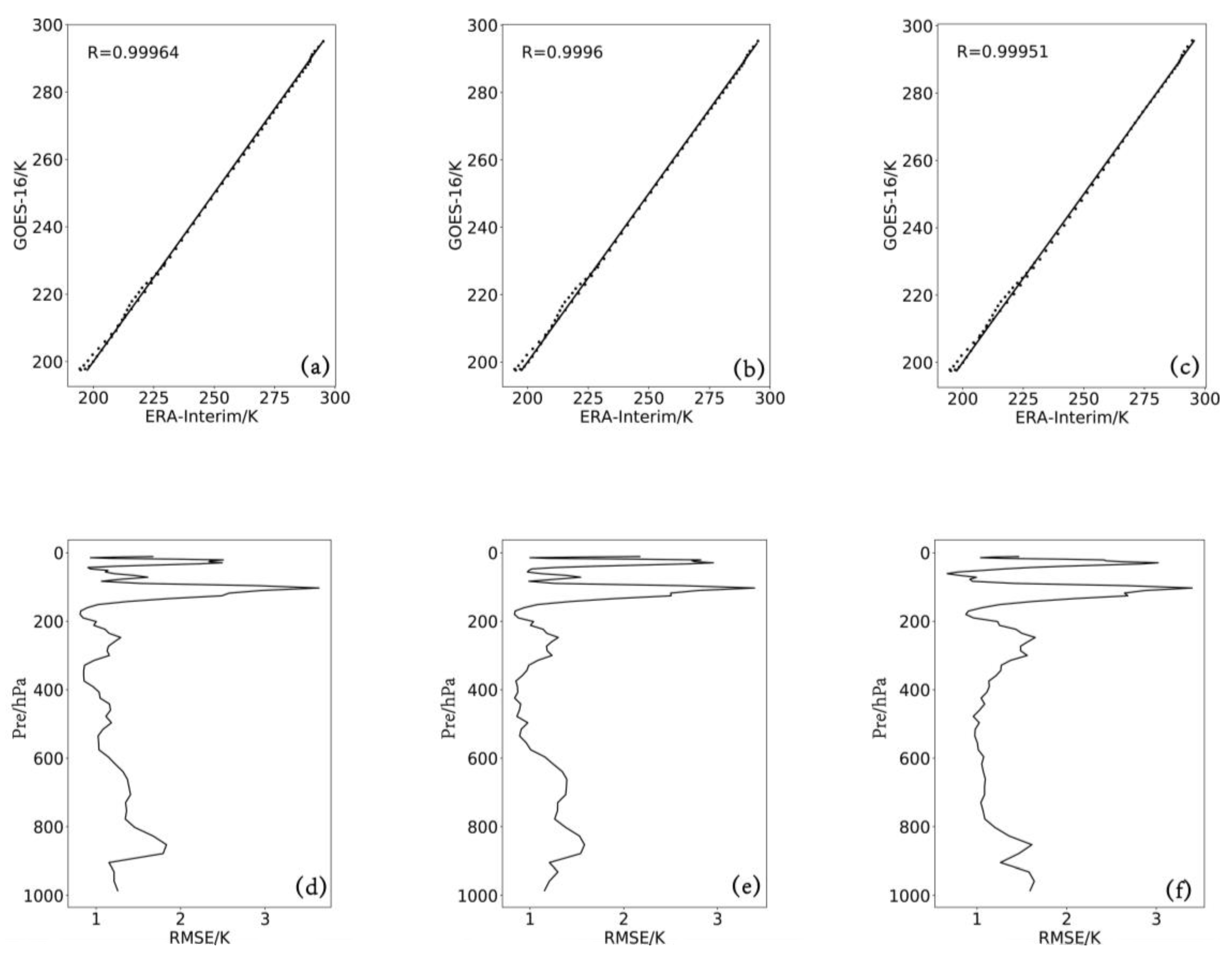
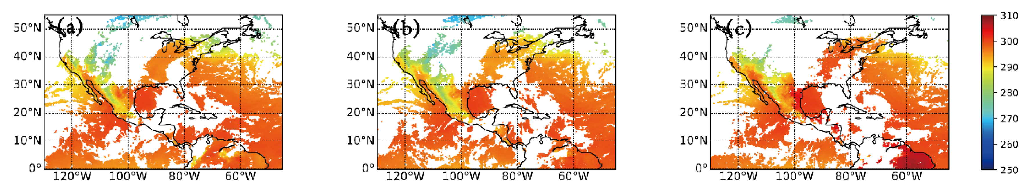
4.1. GOES-16 Atmospheric Temperature-Profile Product Evaluation and Treatment

The observation error of the retrieved data has a certain uncertainty, so it is necessary to evaluate the accuracy of the data before assimilation. Due to the lack of corresponding sounding data in the ocean area, this experiment uses the analysis field data of the European Center for Weather Forecasting (ECMWF) with a horizontal resolution of 0.125° × 0.125°. Compare and verify the 32 layers whose vertical layers are 10–1000 hpa as the “true value”. Choosing the Kwon et al. [33] matching method, find the closest point in time and space distance from the inversion data and ECMWF data, and in the vertical direction, the 32 layers of ECMWF data are interpolated to the 77 layers corresponding to the temperature profile data (10–1000 hpa). Calculate the correlation (Formula (6)) and the root mean square error (Formula (7)), respectively, and use the root mean square error of each layer as the observation error.

$$\mathrm{r}\left(x_i,y_i\right)=\frac{Cov(x_i,y_i)}{\sqrt{\frac{1}{n^2}\sum _{j=1}^n{(x_{ij}-\stackrel{-}{x_i})}^2\sum _{j=1}^n{(y_{ij}-\stackrel{-}{y_i})}^2}}$$

(6)

$$\mathrm{r}\mathrm{m}\mathrm{s}\mathrm{e}\left(\mathrm{i}\right)=\sqrt{\frac{1}{n}{{\displaystyle \sum }}_{j=1}^n\left(x_{ij}-y_{ij}\right)}$$

(7)

Among them, $x$ is the inversion-data value; $y$ is the EC observations value; $i$ is the number of vertical layers; $j$ is the different data points on the same layer; $\stackrel{-}{x_i}$ is the average value of the retrieved data on the $i$ layer; $\stackrel{-}{y_i}$ is the average value of EC observations on the $y$ layer; and $Cov$ represents the covariance of the retrieved data and EC observations.

Figure 2 shows the accuracy evaluation results of the geostationary satellite GOES-16 atmospheric temperature-profile product three times during Hurricane “Michael”. As shown in the figure, the correlation between temperature products and EC data reaches more than 0.99. The RMSE of the temperature profile at the height of 200–1000 hPa is between 0.5 k and 1.8 k. The RMSE is relatively large above 200 hpa, fluctuating between 1.0 k and 3.5 k.

Therefore, in this study, the temperature-profile products between 200 hPa and 1000 hPa are selected for assimilation and prediction experiments. The data above 200 hPa is temporarily not used due to the large error. In order to ensure the quality of the inversion data used for assimilation, strictly select the pixels of “DQF_Overall = 0”, “DQF_Retrieval = 0”, and “DQF_SkinTemp = 0”, and remove the points affected by cloudy sky and precipitation before assimilation. The observation points whose differences between the observation field and the background field are greater than three times the observation standard deviation are eliminated. Taking the height of 1000 hPa as an example, the distribution of the processed data is shown in Figure 3.

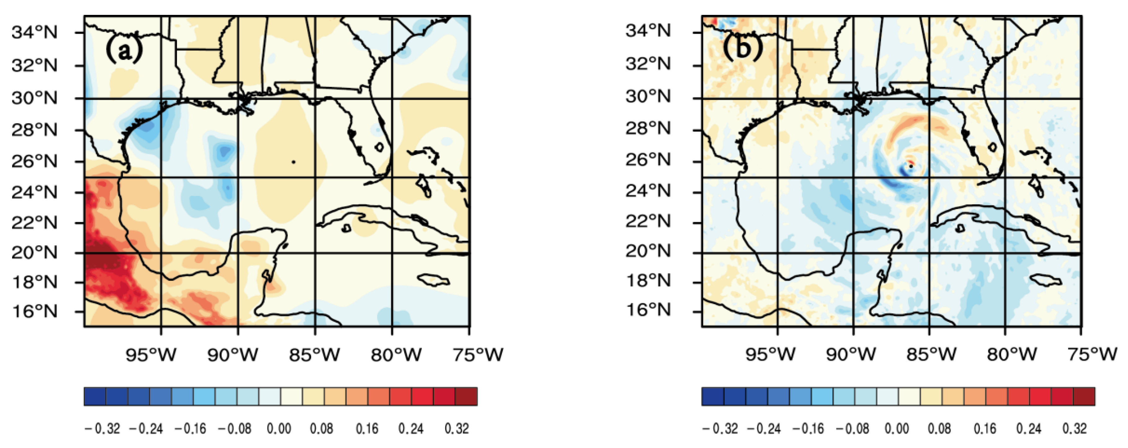
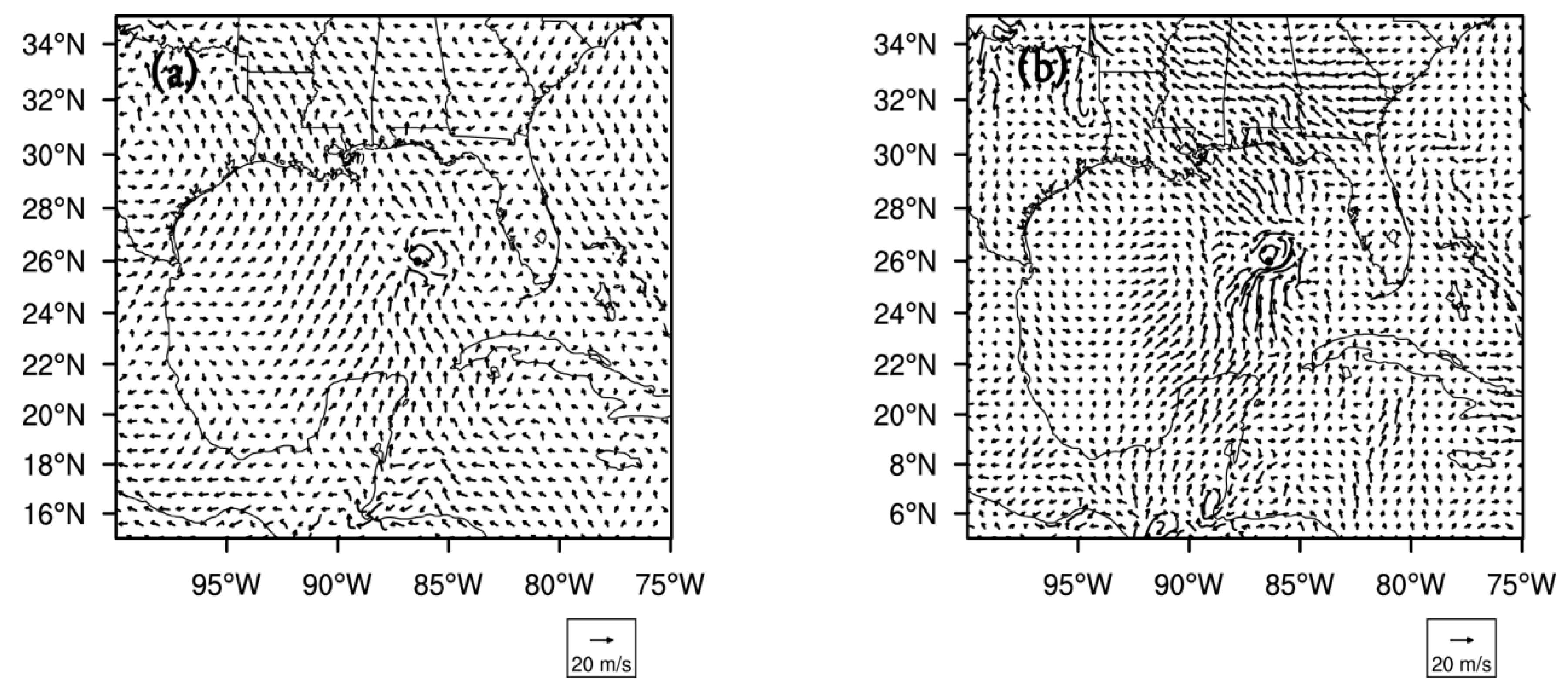
4.2. Increment Analysis

Figure 4 shows the 500 hPa temperature increment of the two groups of assimilation experiments at 18:00 on 9 October 2018. The 3DVar (Figure 4a) shows a large positive increment at the hurricane observation position and a negative temperature increment at the west side of its observation position. The temperature increment structure of the Hybrid (Figure 4b) is very different from that of the 3DVar, with an obvious spiral increment structure around the hurricane, and in the hurricane observation position, it shows a positive temperature increment. Such a spiral structure can better reflect the weather situation. Also, the warm-core structure is conducive to the development of the hurricane, and in terms of thermal mechanism, it will also make the dynamic field adjust accordingly.

Figure 5 shows the 500 hPa wind increment of the two groups of assimilation experiments at the end of the cycle assimilation of the hurricane. It shows that the wind increment of the two groups of experiments is significantly different. The 3DVar (Figure 5a) has a cyclonic wind field increment around the observation position, and all around the cyclonic wind increment, there is a southerly wind field increment, which is conducive to the northward lift of the hurricane. The Hybrid (Figure 5b) has an obvious cyclone increment around the hurricane, and the area with a large increment of the wind field is mainly concentrated around the hurricane, reflecting the obvious localization characteristics of the hybrid assimilation. At the same time, there are northerly wind increments in the south and west of the hurricane observation position, which is favorable for the hurricane to move northerly.

Figure 6 shows the 500 hPa geopotential height increment of the two groups of assimilation experiments at the end of the cycle assimilation of the hurricane. The 3DVar (Figure 6a) has a negative geopotential height increment at the observation position of the hurricane, while the increment is positive both north and east of the observation position. This structure can restrain the hurricane from drifting to the northeast. The geopotential height increment of the Hybrid (Figure 6b) has a distinct spiral structure. In addition, the west side of the observation position is a large-value area with a negative increment, which can promote the westward shift of the hurricane and is conducive to the improvement of the hurricane-track forecast.

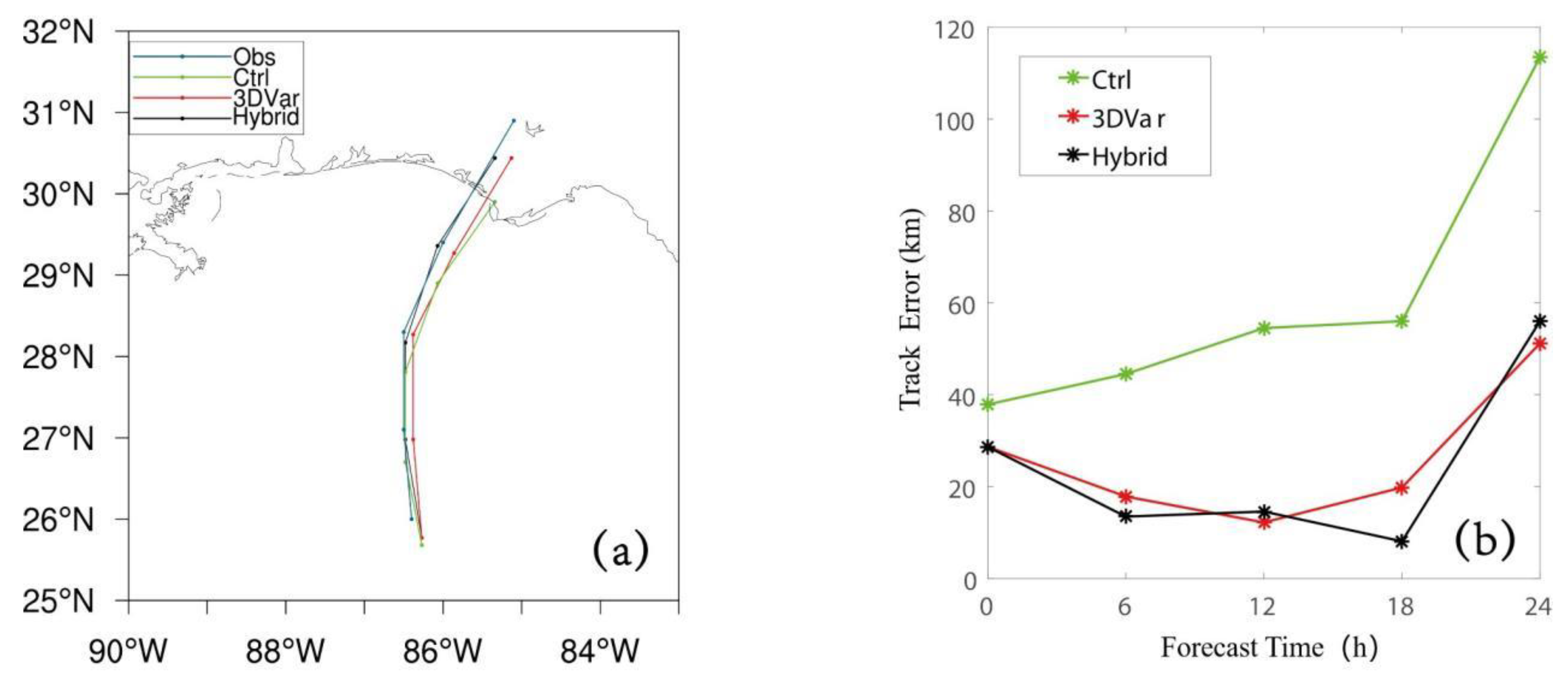
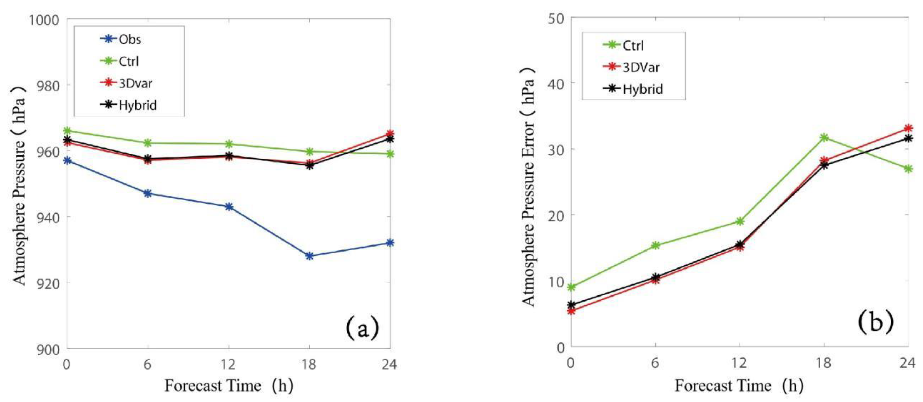
4.3. Track and Intensity Forecast

Figure 7a shows the 24 h hurricane-track forecast, and the observation positions are also plotted. It can be seen that the actual track of the hurricane is northward for the first 12 h, and northeastward for the next 12 h to land in Florida. The Ctrl is located on the southeast side of the observation position at the initial time of the forecast. In the first 6 h, it moves to the northwest, then moves to the north, and then moves to the northeast, and, finally, its landing position is more southerly than the observation position. The 3Dvar moves northwards in the first 12 h, and then moves northeastwards in the following 12 h. Its position is always located to the southeast of the actual observation position, and the landing position is farther south than the observation, but it is obviously better than the Ctrl. The initial position of the Hybrid is located on the southeast side of the observation position. It moves to the northeast direction for the first 6 h, then moves to the northeast direction for the next 6 h, and moves to the northeast direction for the last 12 h. From the forecast of 6 h to 24 h, its moving direction is consistent with the actual observation. At the final landing time, its position is more southwesterly than the actual observation, slightly behind the observation. However, in comparison, the Hybrid is the closest to the observation. The track error (Figure 7b) shows that the misprediction trend of the track of the Ctrl gradually increases, and the maximum error is 113.53 km at 24 h of forecasting. Compared with the Ctrl, the 3DVar has a more obvious improvement on the track forecast, and its track error shows a trend of first decreasing and then increasing, and the smallest track error is 12.21 km at the forecast of 12 h, and the prediction improvement rate is 77.6%. The track error of the Hybrid is to decrease first, then increase, and then decrease and increase. At the forecast of 18 h, there is a minimum track error of 8.6 km, and the improvement rate is 84.9%. In general, the track error of the Hybrid is smaller than that of the 3DVar, and the effect is the best.

The 24 h intensity forecast of Hurricane “Michael” is shown in Figure 8a. The actual observed hurricane intensity tends to increase gradually in the first 18 h and gradually weakens in the last 6 h. The hurricane intensity predicted by the Ctrl gradually increases; the trend of the 3Dvar is similar to that of the Hybrid prediction, and both show increasing at first and then weakening, which are consistent with the actual observation trend. Figure 8b shows that the intensity error of the Ctrl is relatively the largest, and the specific performance is that it gradually increases in the first 18 h and gradually decreases in the last 6 h. The intensity error of the 3DVar increases gradually with the increase of forecast time, and the maximum error is 33.1 hPa when the forecast time is 24 h. The overall error trend of the Hybrid is similar to that of the 3DVar, and in the first 12 h of the forecast, it is slightly larger than the 3DVar. At 12–24 h forecast time, it is slightly smaller than the test 3DVar, and when the forecast time is 24 h, there is the largest error, which is 1.5 hPa smaller than the 3DVar. Overall, both 3Dvar and Hybrid outperform the Ctrl; assimilating the temperature-profile product has less improvement in intensity.

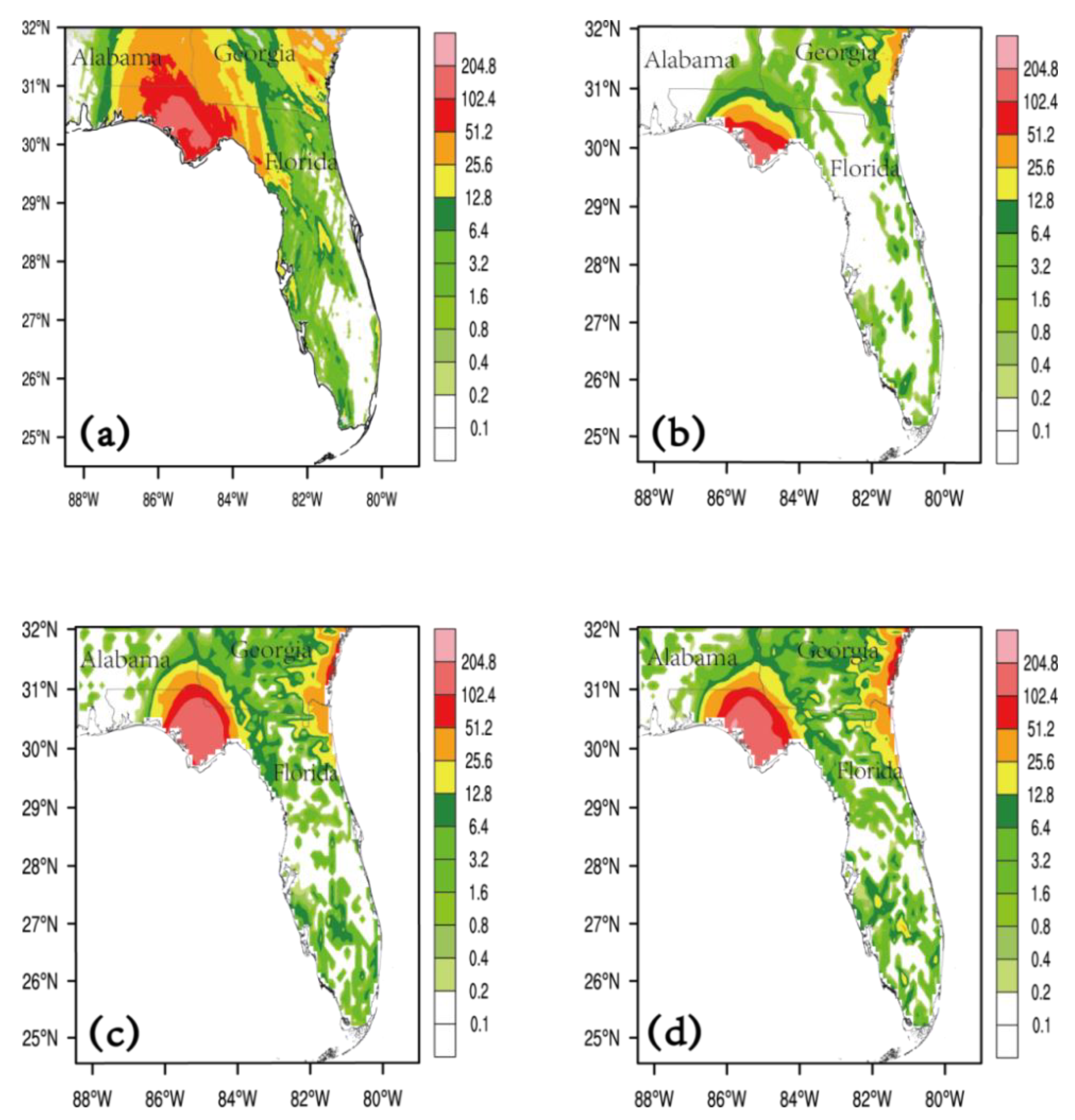
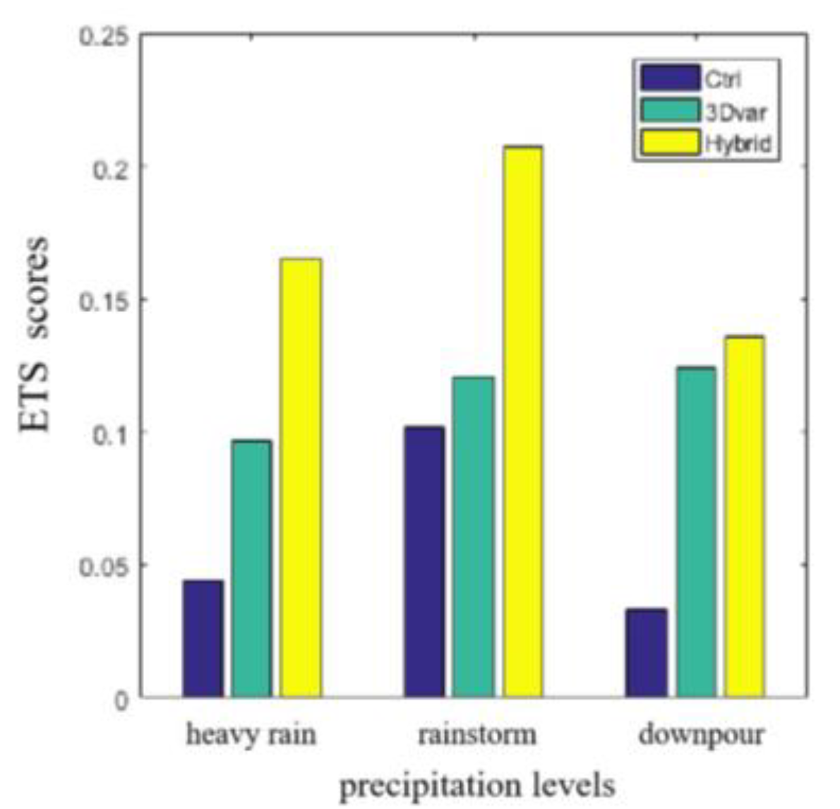
4.4. Precipitation and Equitable Threat Score (ETS) Scores

Figure 9 shows the 24 h accumulated precipitation of Hurricane “Michael” in Florida, southern Alabama, and southern Georgia from 18:00 on 9 October to 18:00 on 10 October. Figure 9a shows the 24 h accumulated precipitation of Stage IV, which is treated as an actual observation. It can be seen that Florida is most affected by precipitation [34], with the highest level of downpour (100–249.9 mm), and local areas are also affected by heavy rain (25.0–49.9 mm) and rainstorms (50.0–99.9 mm). Southern Alabama is also greatly affected by precipitation, mostly heavy rain and rainstorms. Precipitation in Georgia is mainly concentrated in the southwest and eastern coastal areas, and the highest precipitation level is heavy rain. Consistent with the forecast of a southerly track, the area of large precipitation simulated by the Ctrl (Figure 9b) is significantly southerly, mainly concentrated in Florida, and the affected area is small. Precipitation in Georgia and Alabama has not been effectively forecasted. The precipitation simulation of the 3DVar (Figure 9c) for the Florida area is obviously closer to the actual observation than the Ctrl, and the range of the simulated downpour area is significantly expanded. The downpour area shows a north–south trend, but its forecast area is slightly larger than the actual observation. Due to the southerly direction of the track forecast, in Alabama and Southern Georgia, although the downpour is simulated, its influence range is underestimated. In contrast, the precipitation in the Florida region simulated by the Hybrid (Figure 9d) is closest to the actual observation. The predicted trend of the downpour area is northwest–southeast, which is consistent with the observation. And the range of the downpour area is closer to the actual observation than the 3DVar. Also, precipitation in Southern Alabama and Southern Georgia is generally underestimated due to deviations in the final forecast-track position. In general, due to the deviation of the predicted landing position in each experiment, the simulated precipitation area lags behind and deviates to some extent compared with the observed situation. But for Florida, the precipitation intensity and structure simulated by the Hybrid are closer to the actual observation.

Figure 10 shows the ETS scores [35,36] of different precipitation levels in Florida, Alabama, and southern Georgia from 18:00 on 9 October 2018 to 18:00 on 10 October 2018. The Ctrl has the lowest ETS scores for heavy rain, rainstorms, and downpours. The 3DVar has a certain degree of improvement in the ETS scores of different levels of precipitation compared with the Ctrl, and the improvement is the most obvious for downpours. The precipitation forecast of the Hybrid has greatly improved the ETS scores of the three precipitation levels and has better performance than the other two experiments. It shows that the data assimilation of the GOES-16 atmospheric temperature-profile product using the hybrid system can obtain a more accurate precipitation forecast.

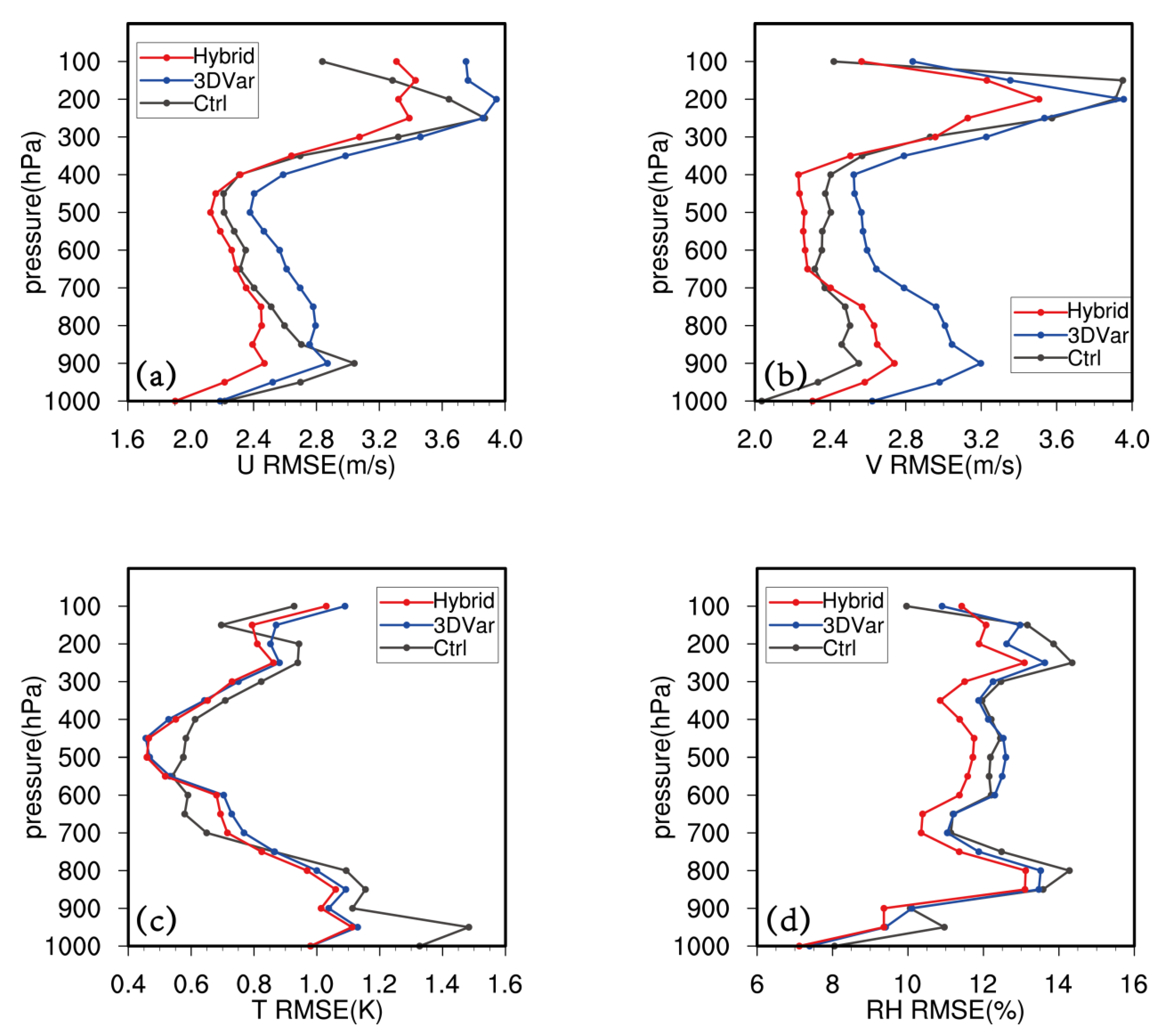
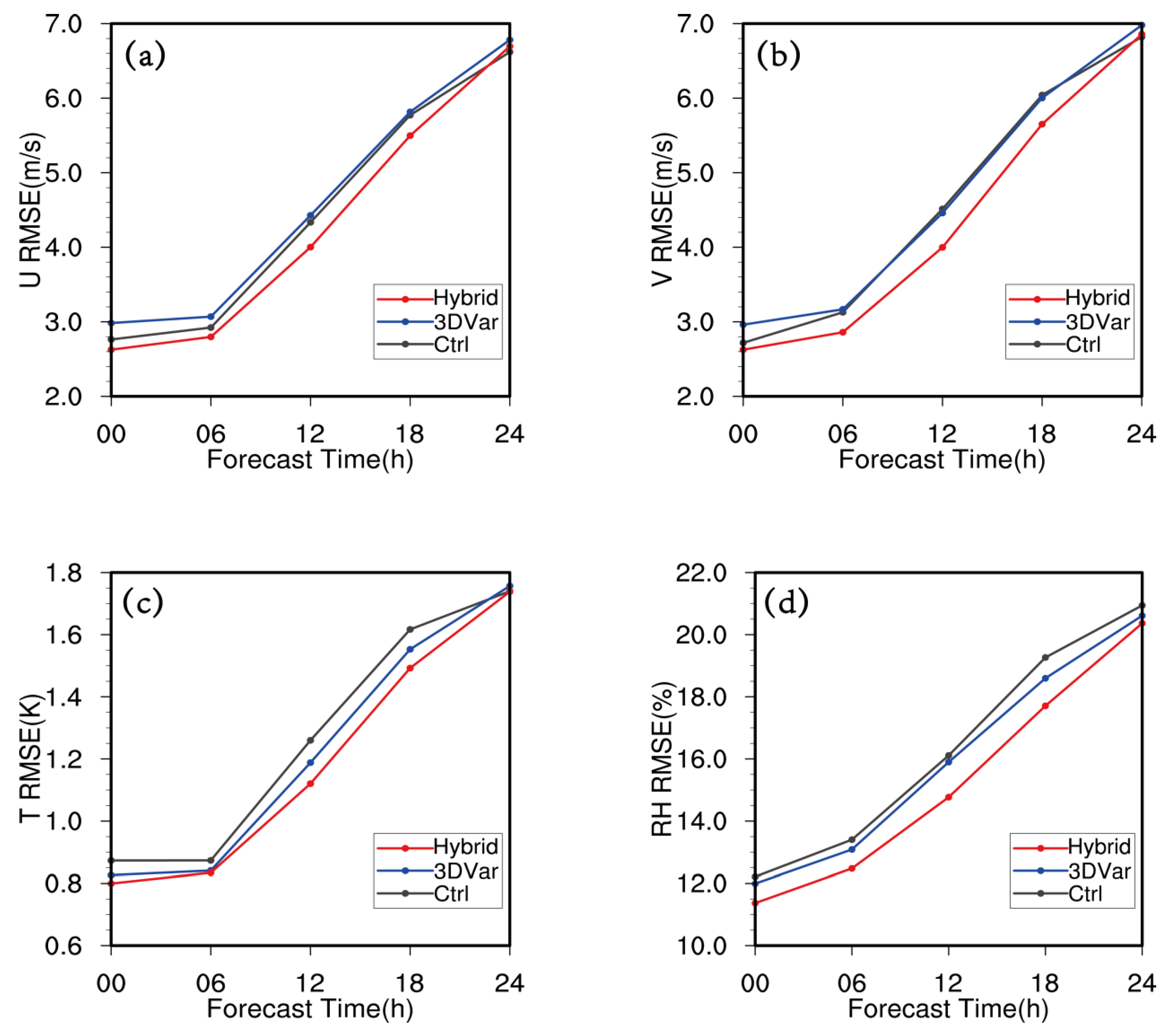
4.5. Root Mean Square Error (RMSE)

In order to further test the performance of the hybrid system, the RMSE of the analysis field at 18:00 on 9 October and the 24 h forecast field, relative to the observation data of different elements, are calculated for the Ctrl, the 3DVar, and the Hybrid, respectively. Figure 11 shows the variation of the average RMSE with the height at 18:00 on 9 October. It was found that, for zonal winds (Figure 11a), the RMSE of the 3DVar is higher than that of the Ctrl. However, the RMSE of the Hybrid is significantly lower. For the meridional wind (Figure 11b), the analysis field of the 3DVar still performs slightly worse. At the height of 1000–700 hPa, the Hybrid is slightly higher than the Ctrl, but lower than the 3DVar, and above the height of 700 hPa, the Hybrid is the lowest compared with the other experiments, and the performance is the best. For temperature (Figure 11c), compared with the Ctrl, the RMSE of the 3DVar is higher at 550–750 hPa heights and lower at the remaining heights, and the overall performance of the Hybrid was slightly better than that of the 3DVar. For relative humidity (Figure 11d), the RMSE of the 3DVar is close to that of the Ctrl, while the RMSE of the Hybrid is obviously the smallest.

Figure 12 shows the variation of the average root mean square error of the forecast field of each element relative to the observation data with the forecast time period. The RMSEs of the zonal winds (Figure 12a) of the three groups of experiments all increased gradually with the increase in forecast time. Among them, the 3DVar performed slightly better than the Ctrl. While the Hybrid remained the lowest, it shows that the Hybrid has the best prediction effect for zonal wind. For meridional winds (Figure 12b), the performance of the 3DVar is not much different from that of the Ctrl, while the RMSE of the Hybrid is consistently the lowest. It also shows that the Hybrid has a positive effect on the forecast of meridional wind. The RMSEs of the three groups of experiments for temperature (Figure 12c) increase continuously with the increase of forecast time. Among them, the RMSE of the Ctrl is the largest, followed by the 3DVar, and the Hybrid is the lowest. It shows that the assimilation of the temperature-profile product has a positive effect on the temperature field, and the hybrid system has a better effect than 3DVar. The RMSEs of the relative humidity in each experiment (Figure 12d) gradually increase. The prediction effect of the 3DVar is slightly better than that of the Ctrl, and the RMSE of the Hybrid is significantly lower than the above two experiments. It shows that using the hybrid system to assimilate the temperature-profile product also has a positive effect on the prediction of the relative humidity field.

5. Conclusions

In this paper, for the actual Hurricane “Michael”, the quality inspection and analysis of the atmospheric temperature profile of the geostationary satellite GOES-16 are carried out. By using the WRF model and the WRFDA assimilation system, the assimilation and prediction experiments are carried out. By increment fields, track and intensity forecasts, precipitation and ETS scores, root mean square error changes with height and forecast time, the effects of the GOES-16 atmospheric temperature profile on hurricane forecasting are analyzed. The main conclusions are as follows:

• Assimilating the GOES-16 atmospheric temperature profile has a good adjustment effect on the model temperature field, wind field, and geopotential height field. The temperature increment of the Hybrid system has an obvious spiral structure. The wind increment concentrated around the hurricane and the adjustment to the geopotential height is also beneficial to the correction of the hurricane position;
• Assimilating the GOES-16 atmospheric temperature profile significantly improves the hurricane-track forecast. And the improvement of the track of the Hybrid is better than that of the 3DVar, and the two assimilation systems have similar prediction effects on the hurricane intensity. Both are better than the Ctrl;
• The 24 h accumulated precipitation and ETS scores show that the simulation of the precipitation structure of the Hybrid is closer to the observation, and its ETS scores are also higher;
• At the end of the cycle assimilation, the Hybrid is the lowest in the root mean square error of each element’s analysis field with the change of height. And its root mean square error with forecast aging is also the most ideal. It shows that the GOES-16 atmospheric temperature profile by the hybrid system can effectively improve the initial field and forecast field of the model.

References

1. Song, L.; Shen, F.; Shao, C.; Shu, A.; Zhu, L. Impacts of 3DEnVar-Based FY-3D MWHS-2 Radiance Assimilation on Numerical Simulations of Landfalling Typhoon Ampil (2018). Remote Sens. 2022, 14, 6037. [Google Scholar] [CrossRef]
2. Shen, F.; Min, J. Assimilating AMSU-A radiance data with the WRF hybrid En3DVAR system for track predictions of Typhoon Megi (2010). Adv. Atmos. Sci. 2015, 32, 1231–1243. [Google Scholar] [CrossRef]
3. Xu, D.; Liu, Z.; Huang, X.Y.; Min, J.; Wang, H. Impact of assimilating IASI radiance observations on forecasts of two tropical cyclones. Meteorol. Atmos. Phys. 2013, 122, 1–18. [Google Scholar] [CrossRef]
4. Liu, Z.; Schwartz, C.S.; Snyder, C.; Ha, S.Y. Impact of Assimilating AMSU-A Radiances on Forecasts of 2008 Atlantic Tropical Cyclones Initialized with a Limited-Area Ensemble Kalman Filter. Mon. Weather Rev. 2012, 140, 4017–4034. [Google Scholar] [CrossRef]
5. Xu, D.; Min, J.; Shen, F.; Ban, J.; Chen, P. Assimilation of MWHS radiance data from the FY-3B satellite with the WRF Hybrid-3DVAR system for the forecasting of binary typhoons. J. Adv. Model. Earth Syst. 2016, 8, 1014–1028. [Google Scholar] [CrossRef]
6. Zhu, T.; Boukabara, S.A.; Garrett, K. Comparing Impacts of Satellite Data Assimilation and Lateral Boundary Conditions on Regional Model Forecasting: A Case Study of Hurricane Sandy (2012). Weather Forecast. 2017, 32, 595–608. [Google Scholar] [CrossRef]
7. Honda, T.; Miyoshi, T.; Lien, G.Y.; Nishizawa, S.; Yoshida, R.; Adachi, S.A.; Terasaki, K.; Okamoto, K.; Tomita, H.; Bessho, K. Assimilating All-Sky Himawari-8 Satellite Infrared Radiances: A Case of Typhoon Soudelor (2015). Mon. Weather Rev. 2018, 146, 213–229. [Google Scholar] [CrossRef]
8. Jones, T.A.; Skinner, P.; Yussouf, N.; Knopfmeier, K.; Reinhart, A.; Wang, X.; Bedka, K.; Smith, W., Jr.; Palikonda, R. Assimilation of GOES-16 Radiances and Retrievals into the Warn-on-Forecast System. Mon. Weather Rev. 2020, 148, 1829–1859. [Google Scholar] [CrossRef]
9. Hartman, C.M.; Chen, X.; Clothiaux, E.E.; Chan, M.Y. Improving the analysis and forecast of Hurricane Dorian (2019) with simultaneous assimilation of GOES-16 all-sky infrared brightness temperatures and tail Doppler radar radial velocities. Mon. Weather Rev. 2021, 149, 2193–2212. [Google Scholar] [CrossRef]
10. Zhang, Y.; Sieron, S.B.; Lu, Y.; Chen, X.; Nystrom, R.G.; Minamide, M.; Chan, M.-Y.; Hartman, C.M.; Yao, Z.; Ruppert, J.H., Jr.; et al. Ensemble-based assimilation of satellite all-sky microwave radiances improves intensity and rainfall predictions for Hurricane Harvey (2017). Geophys. Res. Lett. 2021, 48, e2021GL096410. [Google Scholar] [CrossRef]
11. Li, J.; Huang, H.L. Retrieval of Atmospheric Profiles from Satellite Sounder Measurements by Use of the Discrepancy Principle. Appl. Opt. 1999, 38, 916–923. [Google Scholar] [CrossRef] [PubMed]
12. Li, J.; Wolf, W.W.; Menzel, W.P.; Zhang, W.; Huang, H.L.; Achtor, T.H. Global Soundings of the Atmosphere from ATOVS Measurements: The Algorithm and Validation. J. Appl. Meteorol. 2000, 39, 1248–1268. [Google Scholar] [CrossRef]
13. Weisz, E.; Li, J.; Li, J.; Zhou, D.K.; Huang, H.L.; Goldberg, M.D.; Yang, P. Cloudy sounding and cloud-top height retrieval from AIRS alone single field-of-view radiance measurements. Geophys. Res. Lett. 2007, 34, L12802. [Google Scholar] [CrossRef]
14. Zhou, D.K.; Smith, W.L.; Liu, X.; Larar, A.M.; Mango, S.A.; Huang, H.L. Physically Retrieving Cloud and Thermodynamic Parameters from Ultraspectral IR Measurements. J. Atmos. Sci. 2007, 64, 969–982. [Google Scholar] [CrossRef]
15. Li, J.; Liu, H. Improved hurricane track and intensity forecast using single field-of-view advanced IR sounding measurements. Geophys. Res. Lett. 2009, 36, L11813. [Google Scholar] [CrossRef]
16. Liu, H.; Li, J. An Improvement in Forecasting Rapid Intensification of Typhoon Sinlaku (2008) Using Clear-Sky Full Spatial Resolution Advanced IR Soundings. J. Appl. Meteorol. Climatol. 2010, 49, 821–827. [Google Scholar] [CrossRef]
17. Pu, Z.; Zhang, L. Validation of Atmospheric Infrared Sounder temperature and moisture profiles over tropical oceans and their impact on numerical simulations of tropical cyclones. J. Geophys. Res. Atmos. 2010, 115, D24114. [Google Scholar] [CrossRef]
18. Zheng, J.; Li, J.; Schmit, T.J.; Li, J.; Liu, Z. The impact of AIRS atmospheric temperature and moisture profiles on hurricane forecasts: Ike (2008) and Irene (2011). Adv. Atmos. Sci. 2015, 32, 319–335. [Google Scholar] [CrossRef]
19. Lim, A.H.N.; Nebuda, S.E.; Jung, J.A.; Daniels, J.M.; Bailey, A.; Bresky, W.; Bi, L.; Mehra, A. Optimizing the Assimilation of the GOES-16/-17 Atmospheric Motion Vectors in the Hurricane Weather Forecasting (HWRF) Model. Remote Sens. 2022, 14, 3068. [Google Scholar] [CrossRef]
20. Lee, Y.; Kummerow, C.D.; Zupanski, M. Latent heating profiles from GOES-16 and its impacts on precipitation forecasts. Atmos. Meas. Tech. 2022, 15, 7119–7136. [Google Scholar] [CrossRef]
21. Zhao, Y.; Wang, B. Numerical experiments for Typhoon Dan incorporating AMSU-A retrieved data with 3DVM. Adv. Atmos. Sci. 2008, 25, 692–703. [Google Scholar] [CrossRef]
22. Feng, J.; Qin, X.; Wu, C.; Zhang, P.; Yang, L.; Shen, X.; Han, W.; Liu, Y. Improving Typhoon Predictions by Assimilating the Retrieval of Atmospheric Temperature Profiles from the Fengyun-4a’s Geostationary Interferometric Infrared Sounder (Giirs); Social Science Electronic Publishing: Rochester, NY, USA, 2022. [Google Scholar] [CrossRef]
23. Schmit, T.J.; Gunshor, M.M.; Menzel, W.P.; Gurka, J.J.; Li, J.; Bachmeier, A.S. Introducing the next-generation Advanced Baseline Imager on GOES-R. Bull. Am. Meteorol. Soc. 2005, 86, 1079–10960. [Google Scholar] [CrossRef]
24. Goes-R Series Product Definition and Users’ Guide (Pug). Available online: https://www.ospo.noaa.gov/Organization/Documents/PUG/GS%20Series%20416-R-PUG-Main-0345%20Vol%201%20Rev%202.3.pdf (accessed on 1 January 2019).
25. Ide, K.; Courtier, P.; Ghil, M.; Lorenc, A.C. Unified Notation for data assimilation: Operational, sequential and variational. J. Meteorol. Soc. Jpn. 1997, 75, 181–189. [Google Scholar] [CrossRef]
26. Gu, J.F.; Xiao, Q.N.; Kuo, Y.H.; Barker, D.M.; Xue, J.S.; Ma, X.X. Assimilation and simulation of typhoon Rusa (2002) using the WRF system. Adv. Atmos. Sci. 2005, 22, 415–427. [Google Scholar]
27. Shen, F.; Xue, M.; Min, J. A comparison of limited-area 3DVAR and ETKF-En3DVAR data assimilation using radar observations at convective scale for the prediction of Typhoon Saomai (2006). Meteorol. Appl. 2017, 24, 628–641. [Google Scholar] [CrossRef]
28. Hong, S.Y.; Lim, J.O.J. The WRF single-moment 6-class microphysics scheme (WSM6). J. Korean Meteorol. Soc. 2006, 42, 129–151. [Google Scholar]
29. Mlawer, E.J.; Taubman, S.J.; Brown, P.D.; Iacono, M.J.; Clough, S.A. Radiative Transfer for Inhomogeneous Atmospheres—RRTM, a Validated Correlated-K Model for the Longwave. J. Geophys. Res. Biogeosci. 1997, 102, 16–663. [Google Scholar] [CrossRef]
30. Dudhia, J. Numerical Study of Convection Observed during the Winter Monsoon Experiment Using a Mesoscale Two-Dimensional Model. J. Atmos. 1989, 46, 3077–3107. [Google Scholar] [CrossRef]
31. Noh, Y.; Cheon, W.G.; Hong, S.Y.; Raasch, S. Improvement of the K-profile model for the planetary boundary layer based on large eddy simulation data. Bound. Layer Meteorol. 2003, 107, 401–427. [Google Scholar] [CrossRef]
32. Kain, J.S. The Kain−Fritsch convective parameterization: An update. J. Appl. Meteorol. 2004, 43, 170–181. [Google Scholar] [CrossRef]
33. Kwon, E.H.; Li, J.; Li, J.; Sohn, B.J.; Weisz, E. Use of total precipitable water classification of a priori error and quality control in atmospheric temperature and water vapor sounding retrieval. Adv. Atmos. Sci. 2012, 29, 263–273. [Google Scholar] [CrossRef]
34. Dong, M.; Ji, C.; Chen, F.; Wang, Y. Numerical study of boundary layer structure and rainfall after landfall of Typhoon Fitow (2013): Sensitivity to planetary boundary layer parameterization. Adv. Atmos. Sci. 2019, 36, 431–450. [Google Scholar] [CrossRef]
35. Yu, Z.; Chen, Y.J.; Ebert, B.; Davidson, N.E.; Xiao, Y.; Yu, H.; Duan, Y. Benchmark rainfall verification of landfall tropical cyclone forecasts by operational ACCESS-TC over China. Meteorol. Appl. 2020, 27, e1842. [Google Scholar] [CrossRef]
36. He, B.; Yu, Z.; Tan, Y.; Shen, Y.; Chen, Y. Rainfall forecast errors in different landfall stages of Super Typhoon Lekima (2019). Front. Earth Sci. 2022, 16, 34–51. [Google Scholar] [CrossRef]
Figure 1. The WRF-model domain.
Atmosphere 14 01757 g001
Figure 2. Comparison of correlations (ac) and root mean square errors (df) between ABI-retrieved atmospheric temperature-profile product and ECMWF data during Hurricane “Michael”; ((a,d) are at 06:00 on 9 October 2018, (b,e) are at 12:00 on 9 October 2018, and (c,f) are at 18:00 on 9 October 2018).
Atmosphere 14 01757 g002
Figure 3. Distribution of atmospheric temperature product data at 06:00 (a), 12:00 (b), and 18:00 (c) on 9 October 2018.
Atmosphere 14 01757 g003
Figure 4. The 500hPa temperature increment of Hurricane “Michael” at 18:00 on 9 October 2018 is the observation position of the hurricane; (a) the 3DVar, (b) the Hybrid.
Atmosphere 14 01757 g004
Figure 5. The 500 hPa wind increment of Hurricane “Michael” at 18:00 on 9 October 2018 is the observation position of the hurricane; (a) the 3DVar, (b) the Hybrid.
Atmosphere 14 01757 g005
Figure 6. The 500 hPa geopotential height increment of Hurricane “Michael” at 18:00 on 9 October 2018 is the observation position of the hurricane; (a) the 3DVar, (b) the Hybrid.
Atmosphere 14 01757 g006
Figure 7. The 24 h track forecast and track error of Hurricane “Michael”; (a) track forecast and (b) track error; the initial time is 18:00 on 9 October 2018.
Atmosphere 14 01757 g007
Figure 8. The 24 h intensity forecast and intensity error of Hurricane “Michael”; (a) intensity forecast and (b) intensity error. The initial time is 18:00 on 9 October 2018.
Atmosphere 14 01757 g008
Figure 9. The 24-hour accumulated precipitation of Hurricane “Michael” in Florida, Southern Alabama, and Southern Georgia from 18:00 on 9 October 2018 to 18:00 on 10 October; (a) stage IV observation, (b) the Ctrl, (c) the 3DVar, and (d) the Hybrid.
Atmosphere 14 01757 g009
Figure 10. The 24 h accumulated precipitation for different levels of ETS scores of Hurricane “Michael” in Florida, Southern Alabama, and Southern Georgia from 18:00 on 9 October 2018 to 18:00 on 10 October.
Atmosphere 14 01757 g010
Figure 11. Variation of the root mean square error with the height of the analysis field relative to the observation field at 18:00 on 9 October; (a) zonal wind; (b) meridional wind; (c) temperature; and (d) relative humidity.
Atmosphere 14 01757 g011
Figure 12. Variation of the RMSE of the 24 h forecast field relative to the observation field with time; (a) zonal wind, (b) meridional wind, (c) temperature, and (d) relative humidity.
Atmosphere 14 01757 g012