Twenty-Year Spatiotemporal Variations of TWS over Mainland China Observed by GRACE and GRACE Follow-On Satellites

Abstract

Terrestrial water storage (TWS) is a pivotal component of the global water cycle, profoundly impacting water resource management, hazard monitoring, and agriculture production. The Gravity Recovery and Climate Experiment (GRACE) and its successor, the GRACE Follow-On (GFO), have furnished comprehensive monthly TWS data since April 2002. However, there are 35 months of missing data over the entire GRACE/GFO observational period. To address this gap, we developed an operational approach utilizing singular spectrum analysis and principal component analysis (SSA-PCA) to fill these missing data over mainland China. The algorithm was demonstrated with good performance in the Southwestern River Basin (SWB, correlation coefficient, CC: 0.71, RMSE: 6.27 cm), Yangtze River Basin (YTB, CC: 0.67, RMSE: 3.52 cm), and Songhua River Basin (SRB, CC: 0.66, RMSE: 7.63 cm). Leveraging two decades of continuous time-variable gravity data, we investigated the spatiotemporal variations in TWS across ten major Chinese basins. According to the results of GRACE/GFO, mainland China experienced an average annual TWS decline of 0.32 ± 0.06 cm, with the groundwater storage (GWS) decreasing by 0.54 ± 0.10 cm/yr. The most significant GWS depletion occurred in the Haihe River Basin (HRB) at −2.07 ± 0.10 cm/yr, significantly substantial (~1 cm/yr) depletions occurred in the Yellow River Basin (YRB), SRB, Huaihe River Basin (HHB), Liao-Luan River Basin (LRB), and Southwest River Basin (SWB), and moderate losses were recorded in the Northwest Basin (NWB, −0.34 ± 0.03 cm/yr) and Southeast River Basin (SEB, −0.24 ± 0.10 cm/yr). Furthermore, we identified that interannual TWS variations in ten basins of China were primarily driven by soil moisture water storage (SMS) anomalies, exhibiting consistently and relatively high correlations (CC > 0.60) and low root-mean-square errors (RMSE < 5 cm). Lastly, through the integration of GRACE/GFO and Global Land Data Assimilation System (GLDAS) data, we unraveled the contrasting water storage patterns between northern and southern China. Southern China experienced drought conditions, while northern China faced flooding during the 2020–2023 La Niña event, with the inverse pattern observed during the 2014–2016 El Niño event. This study fills in the missing data and quantifies water storage variations within mainland China, contributing to a deeper insight into climate change and its consequences on water resource management.

1. Introduction

Terrestrial water storage (TWS) encompasses the total water stored in surface water reservoirs, soil moisture, and groundwater, making it a fundamental component of the global hydrological cycle [1,2,3]. TWS significantly influences ecological ecosystems and the occurrence of extreme hydrological events [4,5,6]. Therefore, accurately estimating changes in TWS is crucial for gaining insights into and monitoring a wide range of environmental changes, including climate change, water resource management, and extreme hydrological disasters [7,8]. China, as a nation that has undergone substantial economic growth and population expansion since the implementation of the reform and which includes opening-up market economic policy in the 1970s, is also one of the most water-stressed countries in the world, thus and faces increasing water scarcity challenges [9,10,11]. Monitoring the variability in TWS is not only critical for understanding the intricate interplay between economic development and the rising demand for water resources in China but also aligns with the goals of the national sustainable development policy [12,13].

Since its launch in 2002, the Gravity Recovery And Climate Experiment (GRACE) mission has revolutionized the monitoring of TWS by providing monthly global gravity fields in the form terms of spherical harmonics coefficients [14]. GRACE has proven to be an innovative approach for tracking large-scale changes in TWS, offering distinct advantages over traditional ground-based observations in terms of both temporal and spatial coverage [15,16]. Notable assessments of GRACE-derived TWS have been conducted on continental scales and globally [17,18]. The monthly gravity field estimates from GRACE have achieved geoid height undulation accuracies as fine as 2 to 3 mm at spatial resolutions as small as longer than ~330 km (half-wavelength) [14]. The implementation of GRACE has facilitated numerous studies focused on TWS in mainland China. Further investigations have highlighted the value of GRACE in understanding the dynamics of TWS during extreme events, such as droughts in China’s Yangtze River Basin [19] and precipitation patterns in the Pearl River Basin [20]. Assessments of TWS variability in various regions of China have consistently outperformed hydrological model outputs [21,22,23]. Consequently, satellite gravimetry has become the preferred tool for measuring monthly large-scale TWS changes spanning from April 2002 to June 2017.

Following the retirement decommission of the original GRACE mission in October 2017, the GRACE Follow-On twin-satellite missions (GFO), launched in May 2018, have continued to provide reliable and updated TWS data for diverse applications in hydrology, geology, and oceanography [24,25,26]. Notably, the GRACE Follow-On twin satellites has an experiment Laser Range Interferometry (LRI) satellite-to-satellite instrument, in addition to the K/Ka Band (K-Band) micro-wave ranging instrument as the operational sensor. Additionally, advancements in measurement accuracy and the scientific data system have enhanced the capacity of GRACE Follow-On satellites to detect gravitational variations at much slightly smaller resolutions, allowing for precise continued observations of Earth’s mass transports, despite the early loss of accelerometer on one of the GRACE-FO satellites [27]. Researchers have harnessed GRACE Follow-On data to explore various applications, including the study of thermosphere variations triggered by severe geomagnetic storms [28], and continuing to monitor ice sheet mass loss in Antarctica, revealing cumulative losses in specific regions [29].

However, there are 35 months of missing data over the entire GRACE/GFO observational period (22 missing data points during the GRACE period, 11 between the period of GRACE and GFO, and 2 missing data points in the GFO dataset), posing challenges for continuous gravity field monitoring. To address this data gap, a range of innovative approaches have been employed in previous studies, including alternative data sources, statistical methods, time-series prediction techniques, machine learning models, and deep convolutional neural network models [30,31,32,33,34]. In contrast to the complexity and significant computational requirements of machine learning methods or the use of alternative data sources, this study introduces singular spectrum analysis and principal component analysis (SSA-PCA) as a straightforward and efficient approach for filling the missing data. This method, which has been detailed in Section 2.5 and benefits from published code by Yi and Sneeuw (2020), offers a practical solution to reconstruct continuous TWS data with a minimal computational load [35]. The efficient methodology also affords climate studies and interpretations to link long-term TWS evolutions within China to the various climate episodes.

Although previous studies have successfully calculated TWS using GRACE/GFO data, their focus has often been on specific regions in China, or their investigations have been limited to relatively short time periods without the benefit of complete continuous data. In this study, our primary objectives are to fill the missing data with an easier approach and systematically investigate long-term and continuous spatiotemporal variations in TWS and GWS over mainland China, covering the period from April 2002 to March 2023. This comprehensive analysis not only provides a more profound understanding of long-term trends but also contributes to a better understanding of TWS variations and climate changes on a national scale. The research questions addressed in this study include:

(1)

How can the missing data in the GRACE/GFO observational period be effectively filled using the SSA-PCA approach?

(2)

What are the spatiotemporal variations in TWS and GWS across ten major Chinese basins over a twenty-year period?

(3)

Are there contrasting water storage patterns between northern and southern China during the ENSO events observed by GRACE/GFO?

2. Data and Methods

2.1. Study Area

China’s vast geographical expanse exhibits diverse climatic characteristics. Average annual precipitation exhibits a spatial distribution that contrasts with elevation, ranging from 8 to 2450 mm [36]. As altitude decreases, mean annual temperatures rise from −4 to 20 °C, and evapotranspiration varies across the country, peaking in the southeast at 1400 mm and dropping to a minimum in the northwest at 18 mm [37]. While China enjoys relatively abundant total water resources, the availability of terrestrial water storage (TWS) varies significantly across regions, as does the vulnerability to extreme weather events. In this study, the country’s waters are categorized into ten major river basins according to the China’s zoning principle for water resources (http://www.chinawater.com.cn/, accessed on 15 October 2022), as depicted in Figure 1.

2.2. GRACE/GFO Data

The level-2 data of GRACE/GFO, with spectral resolution up to a degree of 60, are provided by the International Combination Service for Time-Variable Gravity Fields (COST-G), which combines global time-variable gravity field models. These data are available at the International Centre for Global Earth Models (ICGEM) website (http://icgem.gfz-potsdam.de/series/02_COST-G/, accessed on 15 October 2022). The GRACE data span from April 2002 to June 2017, while GFO data cover the period from June 2018 to March 2023. A total of 161 monthly data points is available from GRACE, while 56 monthly data points are obtained from GFO. Notably, there are 22 missing data points during the GRACE period, 11 during the GRACE/GFO overlap, and 2 missing data points in the GFO dataset.

The post-processing of GRACE/GFO data involves several essential steps: (1) Replacing degree-1, C20, and C30 coefficients with values from satellite laser ranging (SLR) [38,39,40]; (2) removing the mean gravity field using the GGM05C mean gravity dataset (http://download.csr.utexas.edu/pub/grace/GGM05/, accessed on 15 October 2022); (3) accounting for glacial isostatic adjustment (GIA) using the recently released ICE-6G D model [41]; (4) minimizing north–south stripe errors with DDK3 filters [42]; (5) converting the filtered spherical harmonic coefficients (SHs) into grids with a resolution of 0.5° × 0.5° [43]; (6) recovering the true signal using the forward modeling method [44,45]; and (7) filling the missing data with the SSA-PCA algorithm, which will be depicted in Section 2.5.

The time-variable gravity field data provided by the gravity satellites can be used to forward compute via Farrell’s loading formalism expressed as the terrestrial water storage (TWS), which is also known as commonly represented in terms of the equivalent water column heigh [44]:

$$\mathrm{T}\mathrm{W}\mathrm{S}=\frac{a{\rho }_a}{3{\rho }_w}\sum _{l=0}^{\mathrm{\infty }} \sum _{m=0}^l {\tilde{P}}_{lm}\left(\cos \theta \right)\frac{2l+1}{1+k_l}\left(\Delta C_{lm}\cos \left(m\lambda \right)+\Delta S_{lm}\sin \left(m\lambda \right)\right)$$

(1)

where a represents the mean radius of the Earth, ${\rho }_a$ is the mean density of the Earth, ${\rho }_w$ is the density of water, $l$ and $m$ correspond to the orders and numbers of the spherical harmonic coefficients, ${\tilde{P}}_{lm}\left(\cos \theta \right)$ denotes the fully specified Legendre conjunction function, $k_l$ is the load love numbers with order $l$, $\Delta C_{lm}$ and $\Delta S_{lm}$ signify the changes in spherical harmonic coefficients, $\theta$ is the calculated geocentric residual latitude, and $l$ stands for the calculated geocentric longitude.

Groundwater storage (GWS) can be calculated by Equation (2):

$$\mathrm{G}\mathrm{W}\mathrm{S}=\mathrm{T}\mathrm{W}\mathrm{S}-\mathrm{S}\mathrm{M}\mathrm{S}$$

(2)

$$\mathrm{S}\mathrm{M}\mathrm{S}=\mathrm{S}\mathrm{M}+\mathrm{S}\mathrm{W}\mathrm{S}+\mathrm{C}\mathrm{W}\mathrm{S}+\mathrm{S}\mathrm{W}\mathrm{E}$$

(3)

SMS represents a comprehensive water storage that incorporates soil moisture (SM), snow water equivalent (SWE), canopy water storage (CWS), and surface water storage (SWS). It is pertinent to note that SM, SWE, CWS, and SWS can be derived from Global Land Data Assimilation System (GLDAS) data. However, due to the limited variability observed in SWS in comparison to SM and its frequent exclusion in previous studies [46,47,48], we also excluded it here.

2.3. GLDAS Data

The NASA Global Land Data Assimilation System (GLDAS) integrates satellite and ground-based observational data to simulate realistic land surface conditions, including soil moisture, temperature, evapotranspiration, and runoff [46]. For this study, we utilized version 2.2 of the GLDAS Noah land surface model to obtain the SM, SWE, CWS, and SWS; these variables can model the comprehensive water storage. GLDAS data can be accessed at https://hydro1.gesdisc.eosdis.nasa.gov/data/GLDAS/, accessed on 15 October 2022.

2.4. ENSO and IOD Index

El Niño/Southern Oscillation (ENSO), a naturally occurring anomalous state of tropical Pacific Ocean atmosphere conditions, stands as the primary predictor for global climate disruptions. In this study, we employed the Multivariate ENSO Index (MEI), which integrates oceanic and atmospheric variables, to precisely quantify the intensity of ENSO events. The latest time series data for MEI.v2 (2002.04–2023.03) is accessible for download on the Physical Sciences Laboratory website (https://psl.noaa.gov/enso/mei/, accessed on 15 October 2022).

Indian Ocean Dipole (IOD) is a climate phenomenon characterized by differences in sea surface temperatures between the eastern and western regions of the Indian Ocean. This natural occurrence exerts a substantial influence on weather patterns and climate across neighboring regions, encompassing parts of Africa, Australia, and China. Access to data related to the IOD, as well as MEI, can be obtained from the Physical Sciences Laboratory website mentioned above.

2.5. Algorithm of Filling Missing Data

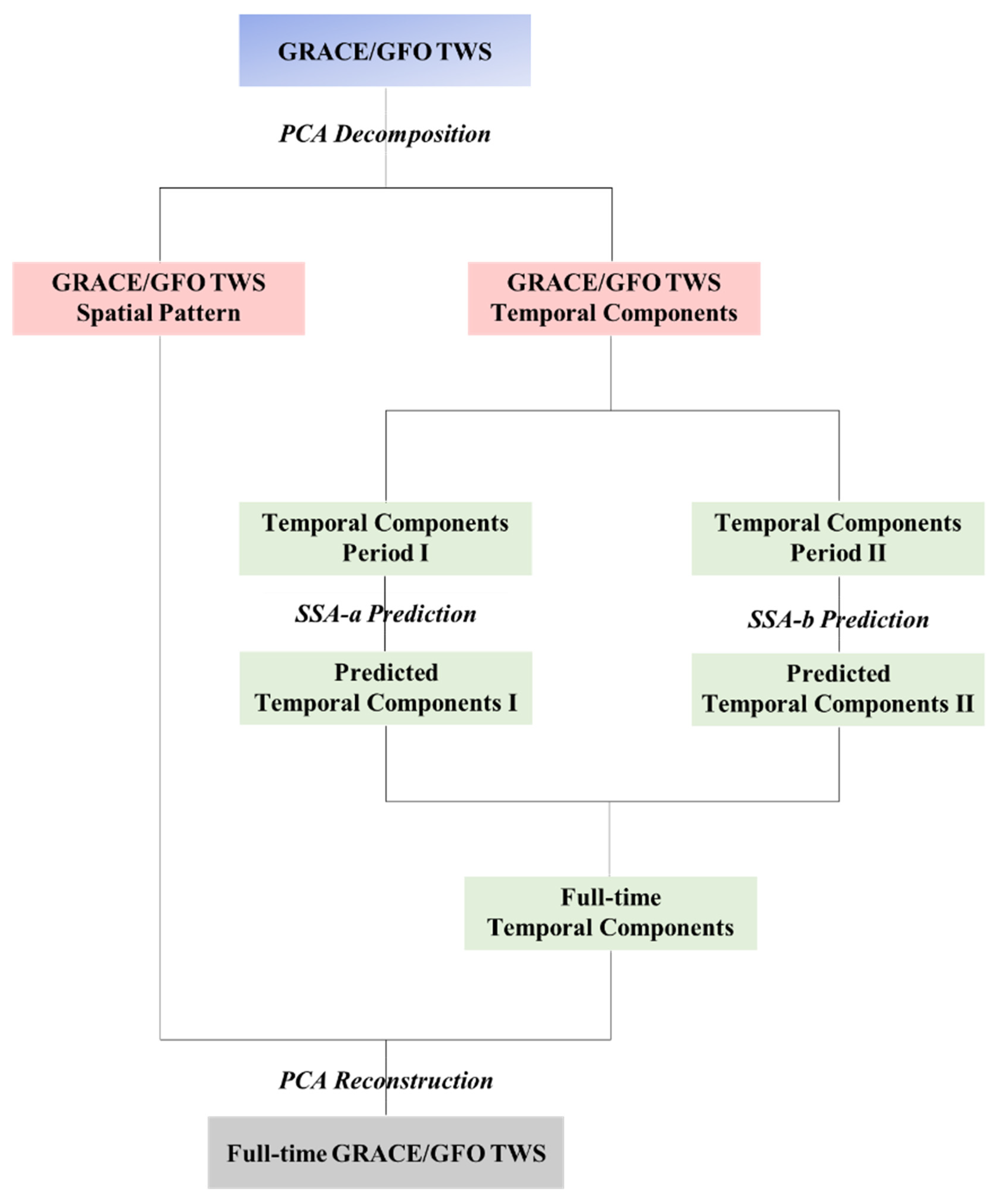
Figure 2 illustrates the detailed procedure for filling missing data. Initially, the gridded TWS dataset underwent decomposition into orthogonal spatial patterns and temporal modes using principal component analysis (PCA) as follows:

$$X_{n\times t}=E_{n\times n}{T}_{n\times t1},$$

(4)

In this equation, the data matrix $X_{n\times t}$ comprises n rows for each spatial grid cell and t columns for each epoch, representing the mean-centered original data. The columns of $E_{n\times n}$ contain the separated spatial patterns, and the rows of $T_{n\times t}$ depict the associated temporal evolution. To retain the total signal variance, we can select the first r dominant modes, as shown in Equation (4):

$$X_{n\times t}=E_{n\times r}{T}_{r\times t1},$$

(5)

Within these r modes, the temporal components are categorized into two distinct periods: period I, which encompasses missing data from April 2002 to June 2017, and period II, spanning from July 2017 to the present. Subsequently, we employed singular spectrum analysis (SSA) to predict these missing data during these two different periods, referred to as SSA-a and SSA-b, respectively. During period I (the period of missing data in the GRACE missions), we employed the SSA-a prediction method to obtain the filled results, while SSA-b was utilized to predict the missing data during period II (the period of missing data after GRACE missions). For a comprehensive understanding of the SSA methodology, please refer to [35]. The predicted modes were derived as follows:

$${\widehat{T}}_{r\times t2}={\widehat{T}}_{r\times ta}+{\widehat{T}}_{r\times tb},$$

(6)

where $T_{r\times ta}$ and $T_{r\times tb}$ are the two predicted time spans that correspond to period I and period II, respectively. Finally, the full-time gridded TWS, ${\widehat{X}}_{n\times t2}$, was reconstructed as follows:

$${\widehat{X}}_{n\times t2}={\widehat{E}}_{n\times r}{\widehat{T}}_{r\times t2}$$

(7)

In this study, we referred to the procedure as SSA-PCA.

2.6. Spatiotemporal Analysis Method

In this study, we employed a harmonic analysis method for time series data to compute trends, seasonal cycles, and interannual variations in ten major river basins of China. The analysis covered the period from April 2002 to March 2023. The mathematical formulation of this method is as follows:

$$\mathrm{Y}=\mathrm{a}·\mathrm{t}+\mathrm{b}1·\cos \left({\omega }_1·\left(\mathrm{t}+{\psi }_1\right)\right)+\mathrm{b}2·\cos \left(2·{\omega }_2·\left(\mathrm{t}+{\psi }_2\right)\right)+\mathsf{\epsilon }$$

(8)

In Equation (8), a represents the trend, b1 and b2 denote the annual amplitude and semi-annual amplitude, and ${\psi }_1$ and ${\psi }_2$ represent the annual phase and semi-annual phase, respectively. ε accounts for interannual variations.

3. Results and Discussion

3.1. Filling the Missing Data through SSA-PCA Algorithm

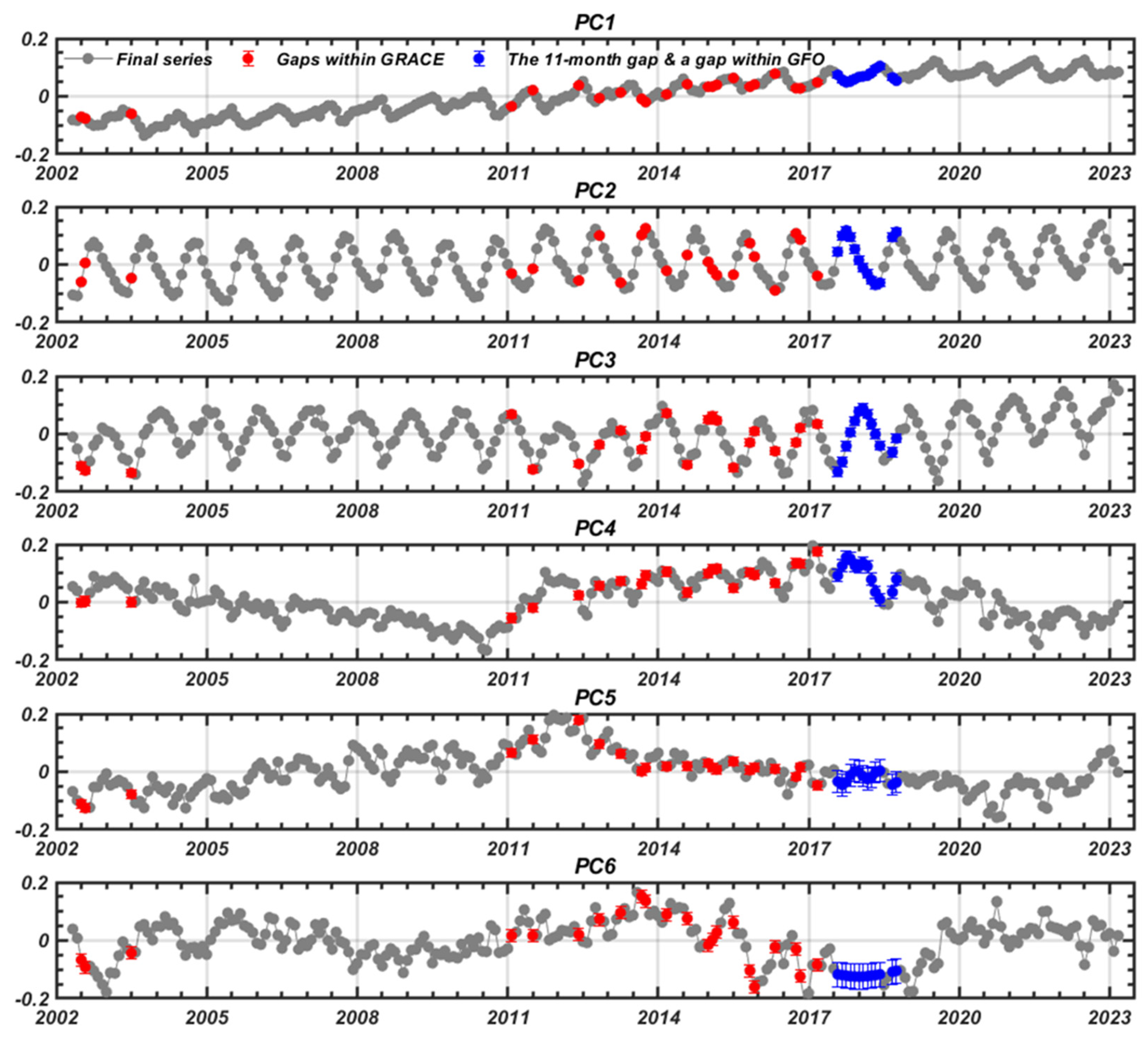
The spatial patterns and temporal components obtained from the PCA decomposition are depicted in Figure 3 and Figure 4, focusing on the first six modes. EOF1, which accounts for 33.1% of the explained variance, exhibits a pattern that closely resembles the overall trend of GRACE/GFO TWS, albeit with some seasonal signals embedded within PC1. Modes 2 (28.4%) and 3 (9.6%) predominantly capture the seasonal variations inherent in the original data, while modes 4, 5, and 6 serve as residual components contributing to the reconstruction of missing data. Employing the SSA-PCA algorithm, this process culminates in the generation of a comprehensive and continuous TWS dataset spanning from April 2004 to March 2023.

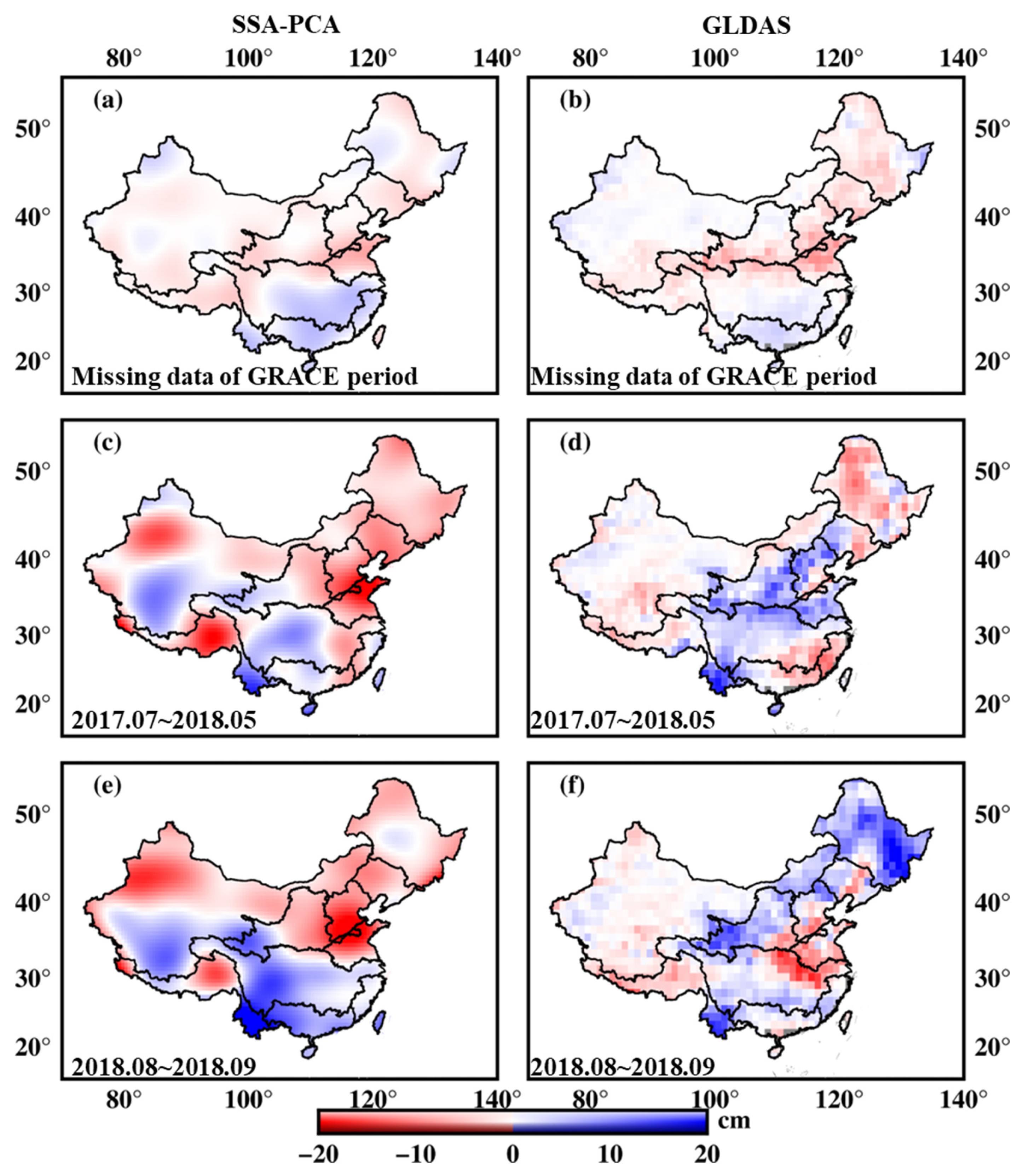
To evaluate the efficacy of the SSA-PCA algorithm in filling missing data, we compared the reconstructed results with water storage estimates derived from GLDAS, as depicted in Figure 5. Over the entire GRACE observational period, the mean values of the filled data demonstrated significant agreement, highlighting elevated water levels in southern China alongside a concurrent decline in water storage in the northern regions. During the intermission between GRACE and GFO missions (July 2017–May 2018), the mean values generated by SSA-PCA closely aligned with those from GLDAS in southern China, the SWB and the SRB. However, during the missing data period of GFO (August 2018–September 2018), some discrepancies emerged in the SRB, while strong agreement persisted in the YTB, SWB, western YRB, and HHB.

Figure 6 presents the correlation coefficient (CC) and root-mean-square error (RMSE) over the entire duration of missing data. In general, most regions exhibited positive CC values within a 95% confidence level, except for the NWB and the middle reaches of the YTB. The RMSE for most regions remained below 15 cm.

Table 1. Correlation coefficient (CC) and root-mean-square error (RMSE) for the comparison between the filled data obtained through SSA-PCA and the results of GLDAS in the ten primary basins of China. These CC values all meet the 95% confidence threshold.

NO.	Name	CC	RMSE (cm)
1	YTB	0.67	3.52
2	YRB	0.41	2.80
3	SRB	0.66	7.63
4	ZRB	0.38	7.52
5	HRB	0.53	5.36
6	HHB	0.24	7.71
7	LRB	0.53	7.12
8	NWB	0.49	1.78
9	SWB	0.71	6.27
10	SEB	0.48	6.51

provides a comprehensive summary of the CC and RMSE values in the ten main basins of China. Notably, the SSA-PCA algorithm demonstrated exceptional performance in the SWB (CC: 0.71, RMSE: 6.27 cm), YTB (CC: 0.67, RMSE: 3.52 cm), and SRB (CC: 0.66, RMSE: 7.63 cm), with CC values surpassing 0.6. Moreover, it delivered comparably satisfactory results in the HRB, LRB, NWB, and SEB, with CC values hovering around 0.50. However, the algorithm exhibited relatively diminished performance in the HHB and ZRB, where CC values fell below 0.40. It is important to note that while the SSA-PCA algorithm may not demonstrate optimal performance in specific regions, we should acknowledge that GLDAS-simulated values typically underestimate GRACE observations due to the inherent limitations of GLDAS, which exclusively models soil moisture storage within a maximum depth of 2.0 m and does not incorporate groundwater dynamics [47,48].

3.2. Spatiotemporal Variations of Water Storage over Mainland China

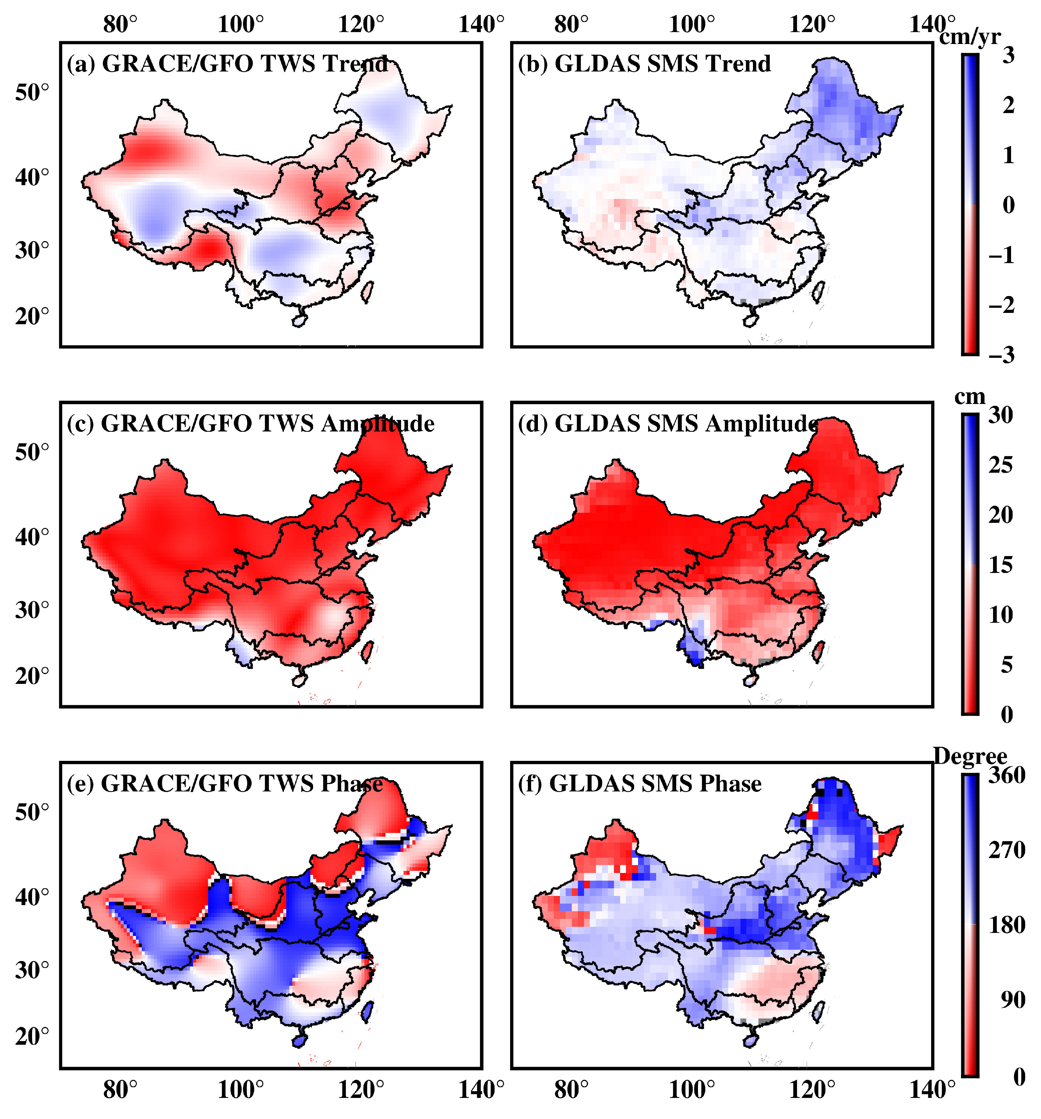
The spatial distribution of trends, annual amplitudes, and annual phases from GRACE/GFO TWS and GLDAS SMS during the period from April 2002 to March 2022 are depicted in Figure 7. In general, mainland China exhibits a decline in GRACE/GFO TWS at a rate of 0.32 ± 0.06 cm/yr, while GLDAS SMS shows a gain at a rate of 0.22 ± 0.08 cm/yr. This indicates a decrease in GWS at a rate of 0.54 ± 0.10 cm/yr. In Figure 7a, GRACE/GFO reveals severe TWS depletion in the HRB (−1.51 ± 0.11 cm/yr), HHB (−1.17 ± 0.12 cm/yr), northern NWB (about −2 cm/yr), and SWB (−1.28 ± 0.05 cm/yr) and a TWS gain in the YTB (0.18 ± 0.06 cm/yr), western YRB (about 0.25 cm/yr), ZRB (0.15 ± 0.10 cm/yr), and southern NWB (about 0.25 cm/yr). In Figure 7b, GLDAS identifies a moderate decrease in SMS in the SWB (−0.16 ± 0.06 cm/yr) and southern NWB (about −0.15 cm/yr), as well as significant increases in the SRB (1.20 ± 0.16 cm/yr), LRB (0.60 ± 0.15 cm/yr), HRB (0.56 ± 0.15 cm/yr), and eastern NWB (about 0.40 cm/yr) and slight increases in the YTB (0.10 ± 0.07 cm/yr), western YRB (about 0.60 cm/yr), and ZRB (0.20 ± 0.10 cm/yr). We also present the GWS trends in ten main basins of China in

Table 2. Trend of TWS, SMS, and GWS in ten main basins over mainland China.

NO.	Name	TWS Trend (cm/yr)	SMS Trend (cm/yr)	GWS Trend (cm/yr)
1	YTB	0.18 ± 0.06	0.10 ± 0.07	0.08 ± 0.04
2	YRB	−0.55 ± 0.05	0.39 ± 0.07	−0.94 ± 0.06
3	SRB	0.10 ± 0.09	1.20 ± 0.16	−1.10 ± 0.10
4	ZRB	0.15 ± 0.10	0.20 ± 0.10	−0.05 ± 0.07
5	HHB	−1.17 ± 0.12	0.01 ± 0.14	−1.18 ± 0.11
6	HRB	−1.51 ± 0.11	0.56 ± 0.15	−2.07 ± 0.10
7	LRB	−0.57 ± 0.11	0.60 ± 0.15	−1.17 ± 0.09
8	NWB	−0.31 ± 0.03	0.04 ± 0.02	−0.34 ± 0.03
9	SWB	−1.28 ± 0.05	−0.16 ± 0.06	−1.12 ± 0.05
10	SEB	−0.14 ± 0.12	0.10 ± 0.12	−0.24 ± 0.10
	Mainland China	−0.32 ± 0.06	0.22 ± 0.12	−0.54 ± 0.10

. The most significant GWS depletion occurred in the HRB at a rate of −2.07 ± 0.10 cm/yr, with substantial decreases in the YRB (−0.94 ± 0.06 cm/yr), SRB (−1.10 ± 0.10 cm/yr), HHB (−1.18 ± 0.11 cm/yr), LRB (−1.17 ± 0.09 cm/yr), and SWB (−1.12 ± 0.05 cm/yr). Moderate losses were observed in the NWB (−0.34 ± 0.03 cm/yr) and SEB (−0.24 ± 0.10 cm/yr). Only the GWS of the YTB showed a slight increase (0.08 ± 0.04 cm/yr). Feng et al. (2013) attributed the GWS depletion of the HHB to a decrease in TWS dominated by deep groundwater [48]. Gong et al. (2018) suggested that increased precipitation in the YTB eliminated GWS overexploitation [49]. Zhong et al. (2018) thought GWS depletion in the LRB was attributed to reduced precipitation and extensive groundwater overexploitation [50]. Xiang et al. (2023) confirmed that the decrease of TWS in the SWB was due to significant glacier mass losses [51].

For annual amplitudes (Figure 7c,d), GRACE/GFO and GLDAS generally exhibited similar spatial patterns, except for the southwest of China, where GLDAS SMS values were notably greater than those of GRACE/GFO TWS. Overall, GLDAS SMS (2.70 ± 0.67 cm) surpassed GRACE/GFO (1.00 ± 0.53 cm) in amplitude. The annual phase of GLDAS closely resembled that of GRACE/GFO, except for regions in the western NWB, eastern NWB, and SRB.

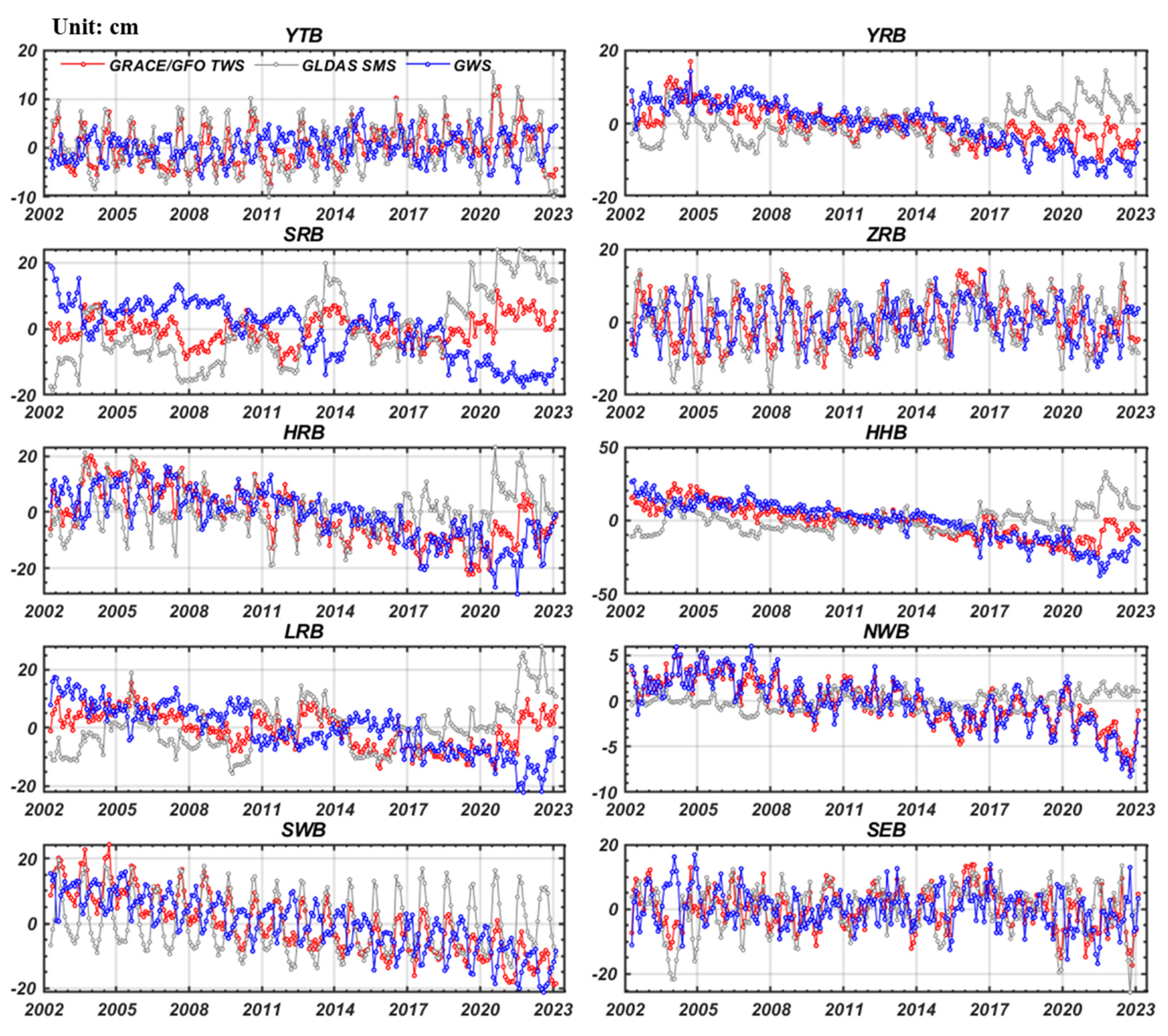
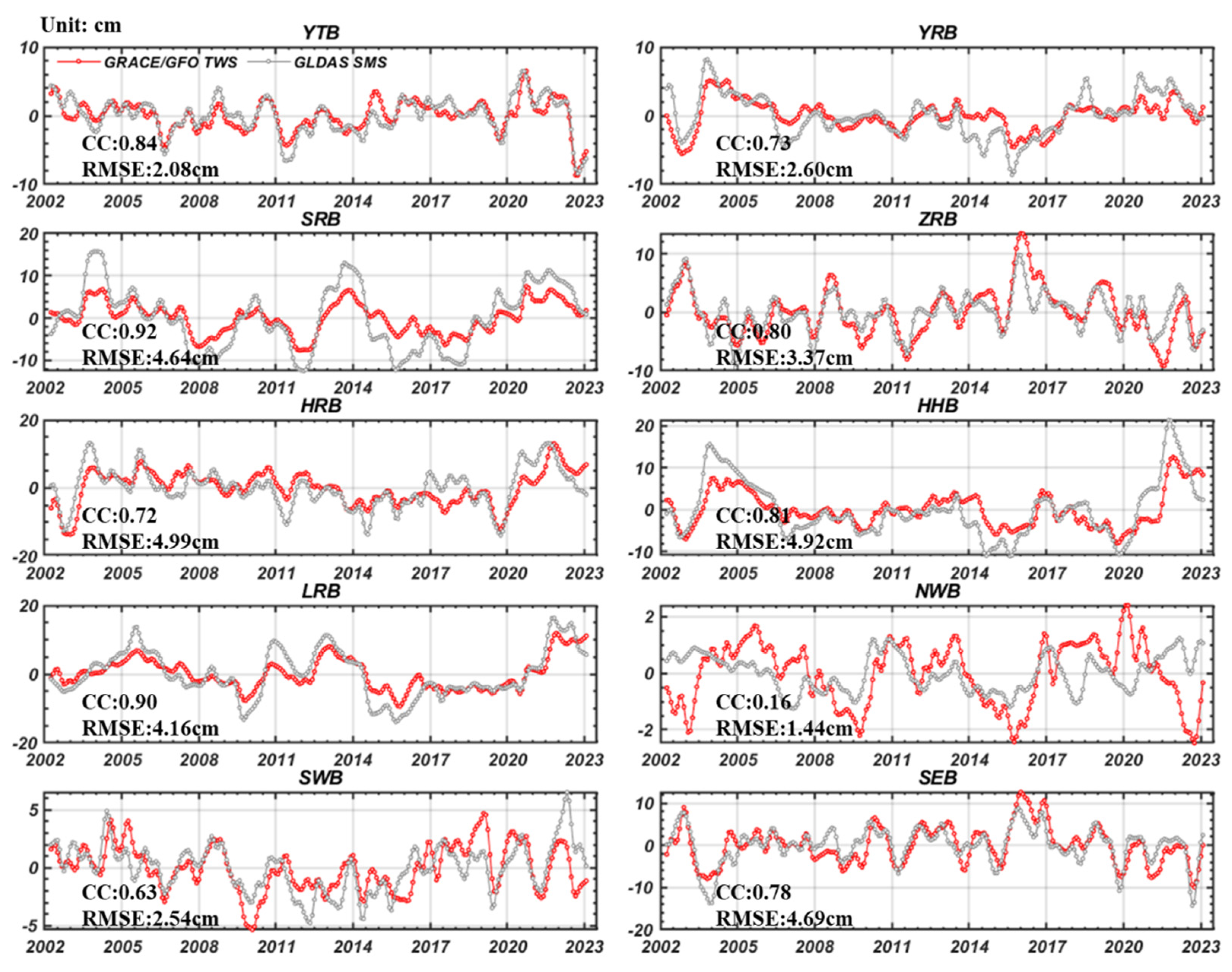
Figure 8 illustrates the continuous twenty-year variations in TWS, SMS, and GWS in the ten main basins of mainland China from April 2002 to March 2023. The southern basins in China (YTB, ZRB, and SWB) exhibited noticeable seasonal variations with one-year and half-year cycles, primarily attributed to seasonal precipitation [19,20,52,53,54] and glacier loss [55,56]. The YRB and HRB showed a pronounced trend of water loss, with GWS trends being predominantly influenced by TWS, showing minimal contribution from SMS. Notably, after 2017, GLDAS revealed an increase in SMS in the YRB and HRB, which can be attributed to the South–North Water Diversion in China [57,58,59,60]. The interannual variations were observed in the SRB, where the decline in GWS is primarily driven by changes in SMS. After removing seasonal terms and trends using the harmonic analysis method, Figure 9 portrays the interannual variations in the ten primary basins; these fluctuations in TWS are primarily attributed to shifts in soil moisture storage (SMS), except in the case of the NWB, consistently exceeding 0.60, with root-mean-square values of less than 5 cm.

3.3. Opposite Status of Water Storage in Northern and Southern China

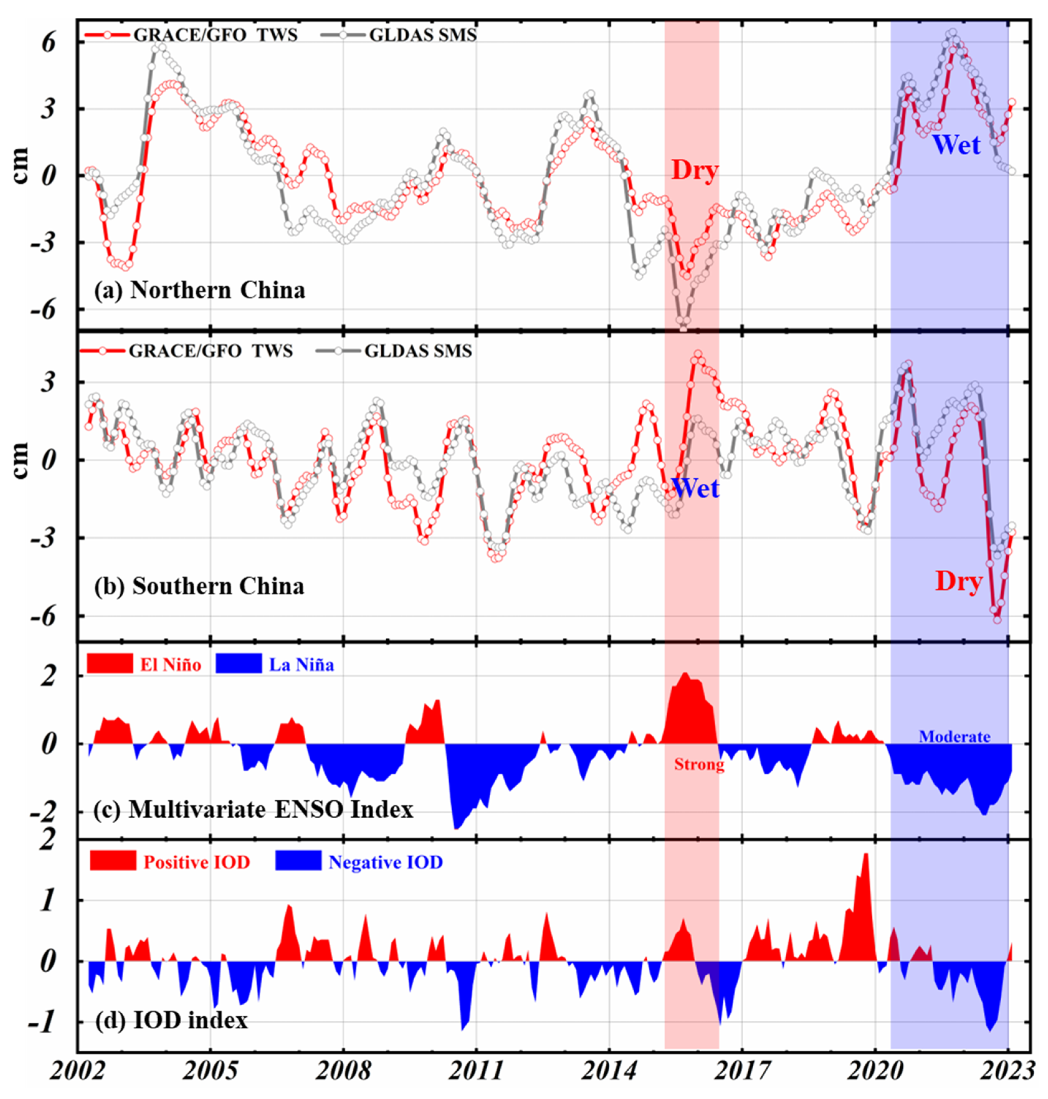
Figure 10a,b presents the interannual time series of water storage in northern and southern China. In this study, we classified the YRB, SRB, HRB, HHB, and LRB as northern China, while the YTB, ZRB, and SEB fell under the southern China category (see Figure 1). In Figure 10c,d, a rare triple-dip La Niña event was observed from June 2020 to February 2023. Concurrently, a negative Indian Ocean Dipole (IOD) event developed from summer 2021 to autumn 2022. In contrast, a strong El Niño event occurred from October 2014 to May 2016, accompanied by a positive IOD event from summer 2015 to autumn 2015. When a positive (negative) IOD coincides with El Niño (La Niña), their impact is typically intensified. China, as a region vulnerable to these climate changes, is significantly affected.

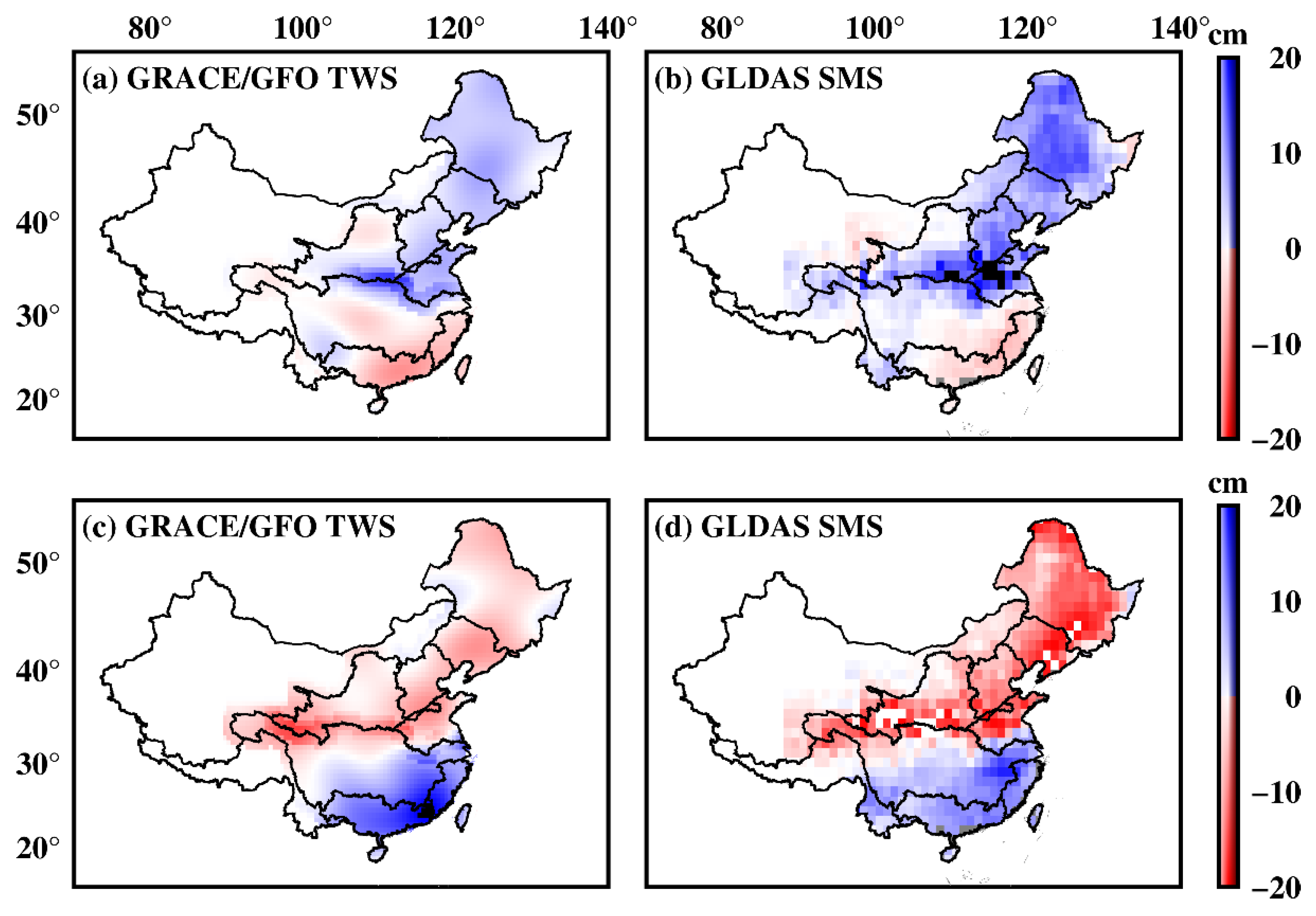
During the 2020–2023 La Niña event, northern China experienced much more water storage, particularly in July 2021, with TWS measuring at 6.16 cm of equivalent water height (EWH), equivalent to approximately 168.78 km³, and SMS at 6.83 cm, amounting to 187.14 km³, when compared to normal conditions. In contrast, southern China witnessed reduced water storage, notably in September 2022, with TWS at −7.01 cm EWH, equivalent to −176.65 km³, and SMS at −4.14 cm EWH, equal to −104.33 km³, compared to normal conditions. The spatial distribution of GRACE/GFO TWS anomalies and GLDAS SMS anomalies across China reveals a reversed pattern (as shown in Figure 11a,b). This pattern is characterized by anti-phased water storage anomalies between southern and northern China, commonly referred to as the “southern drought and northern flooding” pattern. In Section 3.2, we found that the interannual variations in TWS are predominantly attributed to the fluctuations in SMS. GLDAS SMS is simulated within a maximum depth of 2.0 m and is notably influenced by precipitation. During the La Niña years, the northward shift of the subtropical high pressure would foster the development of a rainy atmospheric circulation in northern China during the flood season and cause more rainfall in northern China, which can heighten the risk of flood disasters; conversely, the reduced precipitation in southern China can make these regions more susceptible to drought events [61,62,63].

During the 2014–2016 El Niño event, northern China saw a decrease in water storage, particularly in October 2015, with a TWS of −5.07 cm EWH, equivalent to −138.92 km³, and with an SMS at −7.64 cm EWH, amounting to −209.34 km³, compared to normal conditions. In contrast, southern China observed an increase in water storage, especially in December 2015, with TWS reaching 4.56 cm EWH, equivalent to 114.91 km³, and with SMS reaching 2.13 cm EWH, totaling 53.68 km³, compared to normal conditions. This opposing pattern between northern and southern China is evident in Figure 11c,d, which differs from the results during the 2020–2023 La Niña event and is known as the “southern flooding and northern drought” pattern. In the case of the southern flood and northern drought event, Chen et al. (2020) believed that water storage anomalies exhibited a high correlation with the El Niño Southern Oscillation (ENSO) when considering lagged months [63]. Similarly, Li et al. (2023) demonstrated that both El Niño and specific atmospheric teleconnections, including the Pacific Japan/East Asia Pacific, Eurasia pattern, British–Baikal Corridor pattern, and Silk Road mode, collectively contributed to the dipole pattern of precipitation anomalies [64].

4. Conclusions

In this study, we developed and applied the SSA-PCA algorithm to effectively fill 35 months of missing data spanning from April 2002 to March 2023 in ten major river basins of China. The algorithm consistently demonstrated good performance, as evident from the impressive CC and reasonable RMSE achieved in various basins. Specifically, the SSA-PCA algorithm excelled in the SWB with a CC of 0.71 and an RMSE of 6.27 cm, in the YTB with a CC of 0.67 and an RMSE of 3.52 cm, and in the SRB with a CC of 0.66 and an RMSE of 7.63 cm. Additionally, it provided commendable results in other basins, such as in the HRB with a CC of 0.53 and an RMSE of 5.36 cm, in the LRB with a CC of 0.53 and an RMSE of 7.12 cm, in the NWB with a CC of 0.49 and an RMSE of 1.78 cm, and in the SEB with a CC of 0.48 and an RMSE of 6.51 cm.

Subsequently, our investigation delved into the spatiotemporal dynamics of water storage across mainland China. Notably, mainland China exhibited an overall decline in GRACE/GFO total water storage (TWS) at an annual rate of 0.32 ± 0.06 cm, with groundwater storage (GWS) receding at a rate of 0.54 ± 0.10 cm/yr. This phenomenon was most prominently observed in the HRB, with a substantial GWS depletion rate of 2.07 ± 0.10 cm/yr. Marked reductions of approximately 1 cm/yr were identified in the YRB, SRB, HHB, LRB, and SWB. Moreover, moderate losses were recorded in the NWB at 0.34 ± 0.03 cm/yr and the SEB at 0.24 ± 0.10 cm per year. We also elucidated that interannual variations in the TWS of mainland China, except in the case of the NWB, were predominantly linked to fluctuations in SMS, consistently demonstrating robust CC (>0.60) and minimal RMSE (<5 cm).

Finally, the integration of GRACE/GFO and Global Land Data Assimilation System (GLDAS) data unveiled the fluctuations in water storage in recent ENSO events. Our findings revealed a striking contrast in water storage patterns between northern and southern China. During the 2020–2023 La Niña event, southern China experienced drought conditions, while northern China faced issues of flooding. In stark contrast, the opposite scenario was observed during the 2014–2016 El Niño event.

In conclusion, this study has not only effectively filled the missing data but has also significantly enhanced our understanding of TWS variations in mainland China. These findings hold substantial implications for climate change assessment and water resource management.

References

1. Rodell, M.; Velicogna, I.; Famiglietti, J.S. Satellite-based estimates of groundwater depletion in India. Nature 2009, 460, 999–1002. [Google Scholar] [CrossRef] [PubMed]
2. Huang, Y.; Salama, M.S.; Krol, M.S.; Su, Z.; Hoekstra, A.Y.; Zeng, Y.; Zhou, Y. Estimation of human-induced changes in terrestrial water storage through integration of GRACE satellite detection and hydrological modeling: A case study of the Yangtze River basin. Water Resour. Res. 2015, 51, 8494–8516. [Google Scholar] [CrossRef]
3. Pokhrel, Y.; Felfelani, F.; Satoh, Y.; Boulange, J.; Burek, P.; Gädeke, A.; Gerten, D.; Gosling, S.N.; Grillakis, M.; Gudmundsson, L.; et al. Global terrestrial water storage and drought severity under climate change. Nat. Clim. Chang. 2021, 11, 226–233. [Google Scholar] [CrossRef]
4. Daniel, E.B.; Camp, J.V.; LeBoeuf, E.J.; Penrod, J.R.; Dobbins, J.P.; Abkowitz, M.D. Watershed modeling and its applications: A state-of-the-art review. Open Hydrol. J. 2011, 5, 26–50. [Google Scholar] [CrossRef]
5. Houborg, R.; Rodell, M.; Li, B.; Reichle, R.; Zaitchik, B. Drought indicators based on model-assimilated Gravity Recovery and Climate Experiment (GRACE) terrestrial water storage observations. Water Resour. Res. 2012, 48, W07525. [Google Scholar] [CrossRef]
6. Ndehedehe, C.E.; Awange, J.L.; Corner, R.J.; Kuhn, M.; Okwuashi, O. On the potentials of multiple climate variables in assessing the spatio-temporal characteristics of hydrological droughts over the Volta Basin. Sci. Total Environ. 2016, 557, 819–837. [Google Scholar] [CrossRef] [PubMed]
7. Tapley, B.D.; Watkins, M.M.; Flechtner, F.; Reigber, C.; Bettadpur, S.; Rodell, M.; Sasgen, I.; Famiglietti, J.S.; Landerer, F.X.; Chambers, D.P.; et al. Contributions of GRACE to understanding climate change. Nat. Clim. Chang. 2019, 9, 358–369. [Google Scholar] [CrossRef]
8. Papa, F.; Crétaux, J.F.; Grippa, M.; Robert, E.; Trigg, M.; Tshimanga, R.M.; Kitambo, B.; Paris, A.; Carr, A.; Santos Fleischmann, A.; et al. Water resources in Africa under global change: Monitoring surface waters from space. Surv. Geophys. 2023, 44, 43–93. [Google Scholar] [CrossRef]
9. Zhao, X.; Liu, J.; Liu, Q.; Tillotson, M.R.; Guan, D.; Hubacek, K. Physical and virtual water transfers for regional water stress alleviation in China. Proc. Natl. Acad. Sci. USA 2015, 112, 1031–1035. [Google Scholar] [CrossRef]
10. Feng, K.; Hubacek, K.; Pfister, S.; Yu, Y.; Sun, L. Virtual scarce water in China. Environ. Sci. Technol. 2014, 48, 7704–7713. [Google Scholar] [CrossRef]
11. Sun, S.; Zhou, X.; Liu, H.; Jiang, Y.; Zhou, H.; Zhang, C.; Fu, G. Unraveling the effect of inter-basin water transfer on reducing water scarcity and its inequality in China. Water Res. 2021, 194, 116931. [Google Scholar] [CrossRef]
12. Zhang, Q.; Liu, S.; Wang, T.; Dai, X.; Baninla, Y.; Nakatani, J.; Moriguchi, Y. Urbanization impacts on greenhouse gas (GHG) emissions of the water infrastructure in China: Trade-offs among sustainable development goals (SDGs). J. Clean. Prod. 2019, 232, 474–486. [Google Scholar] [CrossRef]
13. Wang, M.; Janssen, A.B.; Bazin, J.; Strokal, M.; Ma, L.; Kroeze, C. Accounting for interactions between Sustainable Development Goals is essential for water pollution control in China. Nat. Commun. 2022, 13, 730. [Google Scholar] [CrossRef]
14. Tapley, B.D.; Bettadpur, S.; Ries, J.C.; Thompson, P.F.; Watkins, M.M. GRACE measurements of mass variability in the Earth system. Science 2004, 305, 503–505. [Google Scholar] [CrossRef]
15. Scanlon, B.R.; Zhang, Z.; Save, H.; Wiese, D.N.; Landerer, F.W.; Long, D.; Longuevergne, L.; Chen, J. Global evaluation of new GRACE mascon products for hydrologic applications. Water Resour. Res. 2016, 52, 9412–9429. [Google Scholar] [CrossRef]
16. Chen, J.; Cazenave, A.; Dahle, C.; Llovel, W.; Panet, I.; Pfeffer, J.; Moreira, L. Applications and challenges of GRACE and GRACE follow-on satellite gravimetry. Surv. Geophys. 2022, 43, 305–345. [Google Scholar] [CrossRef]
17. Swenson, S.; Wahr, J. Post-processing removal of correlated errors in GRACE data. Geophys. Res. Lett. 2006, 33, L08402. [Google Scholar] [CrossRef]
18. Swenson, S.C. Groundwater depletion in the Middle East from GRACE with implications for transboundary water management in the Tigris-Euphrates-Western Iran region. Water Resour. Res. 2013, 49, 904–914. [Google Scholar] [CrossRef]
19. Zhang, Z.; Chao, B.F.; Chen, J.; Wilson, C.R. Terrestrial water storage anomalies of Yangtze River Basin droughts observed by GRACE and connections with ENSO. Glob. Planet. Chang. 2015, 126, 35–45. [Google Scholar] [CrossRef]
20. Luo, Z.; Yao, C.; Li, Q.; Huang, Z. Terrestrial water storage changes over the Pearl River Basin from GRACE and connections with Pacific climate variability. Geod. Geodyn. 2016, 7, 171–179. [Google Scholar] [CrossRef]
21. Moiwo, J.P.; Yang, Y.H.; Li, H.L.; Han, S.; Hu, Y. Comparison of GRACE within situ hydrological measurement data shows storage depletion in Hai River basin, Northern China. Water SA 2009, 35, 663–670. [Google Scholar] [CrossRef]
22. Long, D.; Shen, Y.; Sun, A.; Hong, Y.; Longuevergne, L.; Yang, Y.; Li, B.; Chen, L. Drought and flood monitoring for a large karst plateau in Southwest China using extended GRACE data. Remote Sens. Environ. 2014, 155, 145–160. [Google Scholar] [CrossRef]
23. Cao, Y.; Nan, Z.; Cheng, G. GRACE gravity satellite observations of terrestrial water storage changes for drought characterization in the arid land of Northwestern China. Remote Sens. 2015, 7, 1021–1047. [Google Scholar] [CrossRef]
24. Ciracì, E.; Velicogna, I.; Swenson, S. Continuity of the mass loss of the world’s glaciers and ice caps from the GRACE and GRACE Follow-on missions. Geophys. Res. Lett. 2020, 47, e2019GL086926. [Google Scholar] [CrossRef]
25. Ghobadi-Far, K.; Han, S.-C.; McCullough, C.M.; Wiese, D.N.; Yuan, D.-N.; Landerer, F.W.; Sauber, J.; Watkins, M.M. GRACE Follow-On Laser Ranging Interferometer Measurements Uniquely Distinguish Short-Wavelength Gravitational Perturbations. Geophys. Res. Lett. 2020, 47, e2020GL089445. [Google Scholar] [CrossRef]
26. Rodell, M.; Reager, J.T. Water cycle science enabled by the GRACE and GRACE-FO satellite missions. Nat. Water 2023, 1, 47–59. [Google Scholar] [CrossRef]
27. Ghobadi-Far, K.; Werth, S.; Shirzaei, M.; Loomis, B.D.; Döhne, T.; Willen, M.O.; Horwath, M. The Impact of New Accelerometer Transplant Data (ACH) on GRACE Follow-On Along-Orbit Inter-Satellite Laser Ranging Observations and Monthly Time-Variable Gravity and Mascon Solutions. J. Geophys. Res. Solid Earth 2023, 128, e2023JB026740. [Google Scholar] [CrossRef]
28. Krauss, S.; Behzadpour, S.; Temmer, M.; Lhotka, C. Exploring thermosphere variations triggered by severe geo-magnetic storm on 26 August 2018 using GRACE Follow-On data. J. Geophys. Res. -Space Phys. 2020, 125, e2019JA027731. [Google Scholar] [CrossRef]
29. Velicogna, I.; Mohajerani, Y.; Geruo, A.; Landerer, F.; Mouginot, J.; Noel, B.; Rignot, E.; Sutterley, T.; van den Broeke, M.; Wessem, M.; et al. Continuity of ice sheet mass loss in Greenland and Antarctica from the GRACE and GRACE Follow-On missions. Geophys. Res. Lett. 2020, 47, e2020GL087291. [Google Scholar] [CrossRef]
30. Lück, C.; Kusche, J.; Rietbroek, R.; Löcher, A. Time-variable gravity fields and ocean mass change from 37 months of kinematic Swarm orbits. Solid Earth 2018, 9, 323–339. [Google Scholar] [CrossRef]
31. Li, W.; Wang, W.; Zhang, C.; Wen, H.; Zhong, Y.; Zhu, Y.; Li, Z. Bridging terrestrial water storage anomaly during GRACE/GRACE-FO gap using SSA method: A case study in China. Sensors 2019, 19, 4144. [Google Scholar] [CrossRef] [PubMed]
32. Li, F.; Kusche, J.; Rietbroek, R.; Wang, Z.; Forootan, E.; Schulze, K.; Lück, C. Comparison of data-driven techniques to reconstruct (1992–2002) and predict (2017–2018) GRACE-like gridded total water storage changes using climate inputs. Water Resour. Res. 2020, 56, e2019WR026551. [Google Scholar] [CrossRef]
33. Sun, Z.; Long, D.; Yang, W.; Li, X.; Pan, Y. Reconstruction of GRACE data on changes in total water storage over the global land surface and sixty basins. Water Resour. Res. 2020, 56, e2019WR026250. [Google Scholar] [CrossRef]
34. Forootan, E.; Schumacher, M.; Mehrnegar, N.; Bezděk, A.; Talpe, M.J.; Farzaneh, S.; Zhang, C.; Zhang, Y.; Shum, C.K. An iterative ICA-based reconstruction method to produce consistent time-variable total water storage fields using GRACE and Swarm satellite data. Remote Sens. 2020, 12, 1639. [Google Scholar] [CrossRef]
35. Yi, S.; Sneeuw, N. Filling the data gaps within GRACE missions using Singular Spectrum Analysis. J. Geophys. Res. Solid Earth 2021, 126, e2020JB021227. [Google Scholar] [CrossRef]
36. Cao, G.; Scanlon, B.R.; Han, D.; Zheng, C. Impacts of thickening unsaturated zone on groundwater recharge in the North China Plain. J. Hydrol. 2016, 537, 260–270. [Google Scholar] [CrossRef]
37. Cheng, M.; Ries, J.C.; Tapley, B.D. Variations of the Earth’s figure axis from satellite laser ranging and GRACE. J. Geophys. Res. Solid Earth 2011, 116, B01409. [Google Scholar] [CrossRef]
38. Sun, Y.; Riva, R.; Ditmar, P. Optimizing estimates of annual variations and trends in geocenter motion and J2 from a combination of GRACE data and geophysical models. J. Geophys. Res. Solid Earth 2016, 121, 8352–8370. [Google Scholar] [CrossRef]
39. Loomis, B.D.; Rachlin, K.E.; Wiese, D.N.; Landerer, F.W.; Luthcke, S.B. Replacing GRACE/GRACE-FO C30 with satellite laser ranging: Impacts on Antarctic Ice Sheet mass change. Geophys. Res. Lett. 2020, 47, e2019GL085488. [Google Scholar] [CrossRef]
40. Peltier, W.R.; Argus, D.F.; Drummond, R. Space geodesy constrains ice age terminal deglaciation: The global ICE-6G_C (VM5a) model. J. Geophys. Res. Solid Earth 2015, 120, 450–487. [Google Scholar] [CrossRef]
41. Kusche, J.; Schmidt, R.; Petrovic, S.; Rietbroek, R. Decorrelated GRACE time-variable gravity solutions by GFZ, and their validation using a hydrological model. J. Geod. 2009, 83, 903–913. [Google Scholar] [CrossRef]
42. Wahr, J.; Molenaar, M.; Bryan, F. Time variability of the Earth’s gravity field: Hydrological and oceanic effects and their possible detection using GRACE. J. Geophys. Res. Solid Earth 1998, 103, 30205–30229. [Google Scholar] [CrossRef]
43. Chen, J.L.; Wilson, C.R.; Seo, K.W. Optimized smoothing of Gravity Recovery and Climate Experiment (GRACE) time-variable gravity observations. J. Geophys. Res. Solid Earth 2006, 111, B06403. [Google Scholar] [CrossRef]
44. Chen, J.L.; Wilson, C.R.; Famiglietti, J.S.; Rodell, M. Attenuation effect on seasonal basin-scale water storage changes from GRACE time-variable gravity. J. Geod. 2007, 81, 237–245. [Google Scholar] [CrossRef]
45. Rodell, M.; Houser, P.R.; Jambor, U.E.A.; Gottschalck, J.; Mitchell, K.; Meng, C.J.; Toll, D. The Global Land Data Assimilation System. Bull. Am. Meteorol. Soc. 2004, 85, 381–394. [Google Scholar] [CrossRef]
46. Ahmed, M.; Abdelmohsen, K. Quantifying modern recharge and depletion rates of the Nubian Aquifer in Egypt. Surv. Geophys. 2018, 39, 729–751. [Google Scholar] [CrossRef]
47. Bonsor, H.C.; Shamsudduha, M.; Marchant, B.P.; Macdonald, A.M.; Taylor, R.G. Seasonal and decadal groundwater changes in African sedimentary aquifers estimated using GRACE products and LSMs. Remote Sens. 2018, 10, 904. [Google Scholar] [CrossRef]
48. Feng, W.; Zhong, M.; Lemoine, J.-M.; Biancale, R.; Hsu, H.; Xia, J. Evaluation of groundwater depletion in North China using the Gravity Recovery and Climate Experiment (GRACE) data and ground-based measurements of groundwater depletion in North China. Water Resour. Res. 2013, 49, 2110–2118. [Google Scholar] [CrossRef]
49. Gong, H.; Pan, Y.; Zheng, L.; Li, X.; Zhu, L.; Zhang, C.; Huang, Z.; Li, Z.; Wang, H.; Zhou, C. Long-term groundwater storage changes and land subsidence development in the North China Plain (1971–2015). Hydrogeol. J. 2018, 26, 1417–1427. [Google Scholar] [CrossRef]
50. Zhong, Y.; Zhong, M.; Feng, W.; Zhang, Z.; Shen, Y.; Wu, D. Groundwater depletion in the West Liaohe River Basin, China and its implications revealed by GRACE and in situ measurements. Remote Sens. 2018, 10, 493. [Google Scholar] [CrossRef]
51. Xiang, L.; Wang, H.; Steffen, H.; Jiang, L.; Shen, Q.; Jia, L.; Su, Z.; Wang, W.; Deng, F.; Qiao, B.; et al. Two Decades of Terrestrial Water Storage Changes in the Tibetan Plateau and Its Surroundings Revealed through GRACE/GRACE-FO. Remote Sens. 2023, 15, 3505. [Google Scholar] [CrossRef]
52. Xu, L.; Chen, N.; Zhang, X.; Chen, Z. Spatiotemporal changes in China’s terrestrial water storage from GRACE satellites and its possible drivers. J. Geophys. Res. Atmos. 2019, 124, 11976–11993. [Google Scholar] [CrossRef]
53. Bai, H.; Ming, Z.; Zhong, Y.; Zhong, M.; Kong, D.; Ji, B. Evaluation of evapotranspiration for exorheic basins in China using an improved estimate of terrestrial water storage change. J. Hydrol. 2022, 610, 127885. [Google Scholar] [CrossRef]
54. Song, C.; Ke, L.; Huang, B.; Richards, K.S. Can mountain glacier melting explain the GRACE-observed mass loss in the southeast Tibetan Plateau: From a climate perspective? Glob. Planet. Chang. 2015, 124, 1–9. [Google Scholar] [CrossRef]
55. Wang, Q.; Yi, S.; Sun, W. The changing pattern of lake and its contribution to increased mass in the Tibetan Plateau derived from GRACE and ICESat data. Geophys. J. Int. 2016, 207, 528–541. [Google Scholar] [CrossRef]
56. Zou, F.; Tenzer, R.; Jin, S. Water storage variations in Tibet from GRACE, ICESat, and hydrological data. Remote Sens. 2019, 11, 1103. [Google Scholar] [CrossRef]
57. Zhang, C.; Duan, Q.; Yeh, P.J.F.; Pan, Y.; Gong, H.; Gong, W.; Guo, X. The effectiveness of the South-to-North Water Diversion Middle Route Project on water delivery and groundwater recovery in North China Plain. Water Resour. Res. 2020, 56, e2019WR026759. [Google Scholar] [CrossRef]
58. Zhang, C.; Duan, Q.; Yeh, P.J.F.; Pan, Y.; Gong, H.; Moradkhani, H.; Guo, X. Sub-regional groundwater storage recovery in North China Plain after the South-to-North water diversion project. J. Hydrol. 2021, 597, 126156. [Google Scholar] [CrossRef]
59. Xiong, J.; Yin, J.; Guo, S.; Yin, W.; Rao, W.; Chao, N.; Abhishek. Using GRACE to Detect Groundwater Variation in North China Plain after South–North Water Diversion. Groundwater 2023, 61, 402–420. [Google Scholar] [CrossRef]
60. Jin, H.; Liang, R.; Wang, Y.; Tumula, P. Flood-runoff in semi-arid and sub-humid regions, a case study: A sim-ulation of Jianghe watershed in northern China. Water 2015, 7, 5155–5172. [Google Scholar] [CrossRef]
61. Zhou, Q.; Leng, G.; Huang, M. Impacts of future climate change on urban flood volumes in Hohhot in northern China: Benefits of climate change mitigation and adaptations. Hydrol. Earth Syst. Sci. 2018, 22, 305–316. [Google Scholar] [CrossRef]
62. Yang, L.; Yang, Y.; Villarini, G.; Li, X.; Hu, H.; Wang, L.; Tian, F. Climate more important for Chinese flood changes than reservoirs and land use. Geophys. Res. Lett. 2021, 48, e2021GL093061. [Google Scholar] [CrossRef]
63. Chen, W.; Zhong, M.; Feng, W.; Zhong, Y.; Xu, H. Effects of two strong ENSO events on terrestrial water storage anomalies in China from GRACE during 2005–2017. Chin. J. Geophys. 2020, 63, 141–154. (In Chinese) [Google Scholar] [CrossRef]
64. Li, Z.; Yang, Q.; Yuan, D.; Lu, E.; Ma, Z. Causes of a Typical Southern Flood and Northern Drought Event in 2015 over Eastern China. Adv. Atmos. Sci. 2023, 40, 2092–2107. [Google Scholar] [CrossRef]
Figure 1. Ten main river basins across mainland China.
Atmosphere 14 01717 g001
Figure 2. The procedure of filling the data gap using SSA-PCA. Period I denote the period of missing data in GRACE missions, and period II is the period of missing data after GRACE missions.
Atmosphere 14 01717 g002
Figure 3. (af) The first 6 empirical orthogonal functions (EOFs) resulting by the PCA decomposition. The value represents the explained variance.
Atmosphere 14 01717 g003
Figure 4. The first 6 principal components (PCs) resulting from the PCA decomposition. The gray dot line represents the original components, the red line indicates the temporal components I during the GRACE period by SSA-a, and the blue line illustrates the temporal components II after the GRACE period by SSA-b.
Atmosphere 14 01717 g004
Figure 5. Comparisons of the filled data by SSA-PCA and the results of GLDAS at GRACE missions (a,b), July 2017–May 2018 (c,d), August 2018–September 2018 (e,f).
Atmosphere 14 01717 g005
Figure 6. (a) Correlation coefficient (CC) and (b) root-mean-square error (RMSE) between the filled data obtained through SSA-PCA and the corresponding results from GLDAS, spanning the entire period of missing data. The gray-shaded region indicates cases where the CC values do not meet the 95% confidence threshold.
Atmosphere 14 01717 g006
Figure 7. Spatial distribution of the (a) GRACE/GFO TWS trend, (b) GLDAS SMS trend, (c) GRACE/GFO TWS annual amplitude, (d) GLDAS SMS annual amplitude, (e) GRACE/GFO TWS annual phase, and (f) GLDAS SMS annual phase across mainland China.
Atmosphere 14 01717 g007
Figure 8. Temporal variations in water storage in ten main basins over mainland China; the red line represents the time series of GRACE/GFO TWS, the gray line corresponds to GLDAS SMS, and the blue line depicts GWS.
Atmosphere 14 01717 g008
Figure 9. Interannual variations in water storage in ten main basins over mainland China; the red line represents the time series of GRACE/GFO TWS, and the gray line corresponds to GLDAS SMS.
Atmosphere 14 01717 g009
Figure 10. Interannual timeseries of GRACE/GFO TWS and GLDAS SMS in northern (a) and southern (b) China. Parts (c,d) are the multivariate ENSO index and IOD index, respectively.
Atmosphere 14 01717 g010
Figure 11. The interannual spatial pattern of GRACE/GFO TWS during the 2020–2023 La Niña (a) and 2014–2016 El Niño periods (c); and GLDAS SMS during the 2020–2023 La Niña (b) and 2014–2016 El Niño periods (d).
Atmosphere 14 01717 g011