Article

Numerical Simulation on Wind Speed Amplification of High-Rise Buildings with Openings

1
School of Civil Engineering, Changsha University of Science and Technology, Changsha 410114, China
2
Key Laboratory of Safety Control of Bridge Engineering Ministry of Education, Changsha University of Science and Technology, Changsha 410114, China
*
Authors to whom correspondence should be addressed.
Atmosphere 2023, 14(11), 1687; https://doi.org/10.3390/atmos14111687
Submission received: 5 July 2023 / Revised: 29 August 2023 / Accepted: 17 October 2023 / Published: 14 November 2023
(This article belongs to the Special Issue Advances in Computational Wind Engineering and Wind Energy)

Abstract

:
To explore the influence of openings on wind loads and wind speeds in high-rise buildings, the wind flow around three-dimensional (3D) square cylinders with a breadth/height aspect ratio of 1:6 was numerically simulated using the large eddy simulation (LES) method via the Fluent 15.0 platform. The opening measures in the X-direction, Y-direction and both directions were all taken into consideration. Firstly, the inflow turbulence synthesis method and parameter settings for LES were verified by comparing the simulation results of standard square cylinders with those of wind tunnel experiments, and the optimal boundary conditions were determined. Then, the wind speed was extracted and compared with the mean wind speed of incoming flow at the same height to analyze the influence of different opening measures on the wind speed of incoming flow by setting monitoring points in the open holes. Finally, the mechanism underlying the effect of the opening form on wind loads and wind speeds was analyzed from the perspective of time-averaged and transient flow field. The results show that the X-direction openings affect the magnitude and distribution of the surface wind pressures by changing the flow separation and flow reattachment. The narrow tube effect can significantly increase the wind speed, while the Y-direction openings have no obvious improvement effect on the surface wind pressures of the structure. The wind speeds in the open holes are greatly reduced due to the shielding effect, and the wind pressures are also reduced for the Y-direction openings. In the X-direction opening holes, the wind speed at the monitoring point increases, while it decreases in the crosswind open holes. In general, the measure of openings in the X-direction can greatly improve the wind load of the structure compared to openings in the Y-direction, and it can provide a good reference for wind power generation in high-rise buildings.

1. Introduction

Due to the global energy shortage and environmental deterioration, the development of a low-carbon economy and low-carbon cities has become a new trend of social transformation. The construction industry accounts for one third of the national energy consumption, so the design of low-carbon buildings is an important link in the construction of low-carbon cities. It has been reported that if the energy efficiency of buildings is greatly improved and the carbon emissions of buildings are reduced, the construction industry will save about 100–300 million tons of oil-equivalent energy by 2030 and reduce 600–700 million tons of carbon dioxide emissions every year [1]. Hence, in the strategy of vigorously developing low-carbon cities, the exploitation and utilization of new renewable energy is an effective way.
As a sort of non-polluting, renewable and inexhaustible clean energy, wind energy has attracted widespread attention all over the world. Many scholars have conducted similar studies on the wind environment of buildings [2,3,4]. As early as 1997, Stathopolous [5] studied the specific influence of a building surface on the magnitude and direction of ambient wind speed and variation in the flow field. Tamura et al. [6], Murakami et al. [7], Larson [8] and other scholars investigated the interaction between buildings and incoming flow and analyzed the influence of the interference effect of building groups on their environment [9]. As a traditional method of wind energy utilization, wind power generation is of great significance to the development of green buildings with low energy consumption [10,11]. In 1988, the European Commission carried out the “Wind Energy in the Built Environment” (WEBE) research project, which first introduced wind power generation into urban projects [12].
In recent years, to reduce wind loads and wind-induced responses, many aerodynamic measures have been conducted on super high-rise buildings, such as corner modification [13,14,15], opening measures and spoiler settings. Among them, the effect of openings on high-rise buildings has been widely studied. The Pearl River Tower, located in Guangzhou, which is equipped with wind turbines in four open tunnels at two different height levels for power generation, is considered to be an innovative structure [16]. Li et al. investigated the effect of wind load and wind speed amplification in the Pearl River Tower via wind tunnel tests and wind climate data analyses [17,18], as shown in Figure 1. It has been proven that openings have a significant impact on the wind load of high-rise buildings and wind speed amplification. To avoid noise harm from airflow caused by the presence of openings and wind turbines in the Pearl River Tower, Lu et al. analyzed the noise distribution of the open holes and wind turbines in the Pearl River Tower using a numerical simulation method based on the SST k-ε turbulence model [19]. The CFD (Computational Fluid Dynamics) numerical simulation method makes up for its disadvantages of high costs and restrictive conditions in wind tunnel experiments by being a convenient and effective research method. Chen et al. combined wind tunnel tests and numerical simulation methods to investigate the wind effect of high-rise buildings with openings via the Fluent 15.0 platform using the SST k-ε turbulence model, and they obtained the mean wind pressure coefficient and air flow characteristics [20]. By adjusting the duct diameter (d0/d) and the fillet radius of the duct entrance and exit (r/d0), Ruiz et al. [21] evaluated the performance on the basis of average wind speed (U/U0) and turbulent kinetic energy (k/k0) ratios using the 3D steady RANS method, adding to the knowledge on wind energy harvesting of high-rise buildings.
Compared to the method of RANS (Reynolds-Averaged Navier–Stokes), large eddy simulation (LES) based on the spatial-averaged method is more effective in capturing pulsation information of the flow field. Due to its better applicability in analyzing the influence mechanism of wind flow, LES has been widely used in the field of structural wind engineering [22,23,24]. Based on the LES method, this study investigated the wind load and wind speed amplification of high-rise buildings with different opening patterns, including openings in the X-direction, Y-direction and both directions. The effects of opening measures on the influence mechanism of wind speed in high-rise buildings were analyzed. This study aims to provide a useful reference for wind power generation and wind energy utilization for high-rise buildings with openings in the future.

2. CFD Verification and Validation

2.1. Numerical Setups

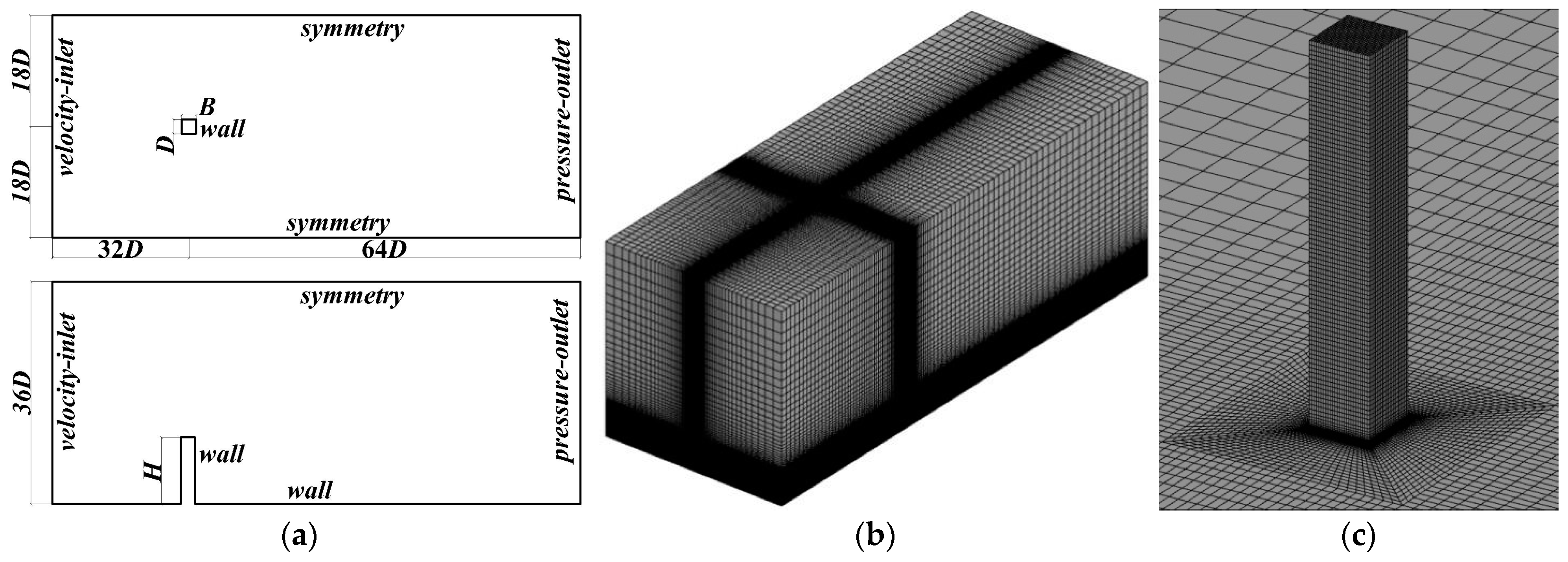
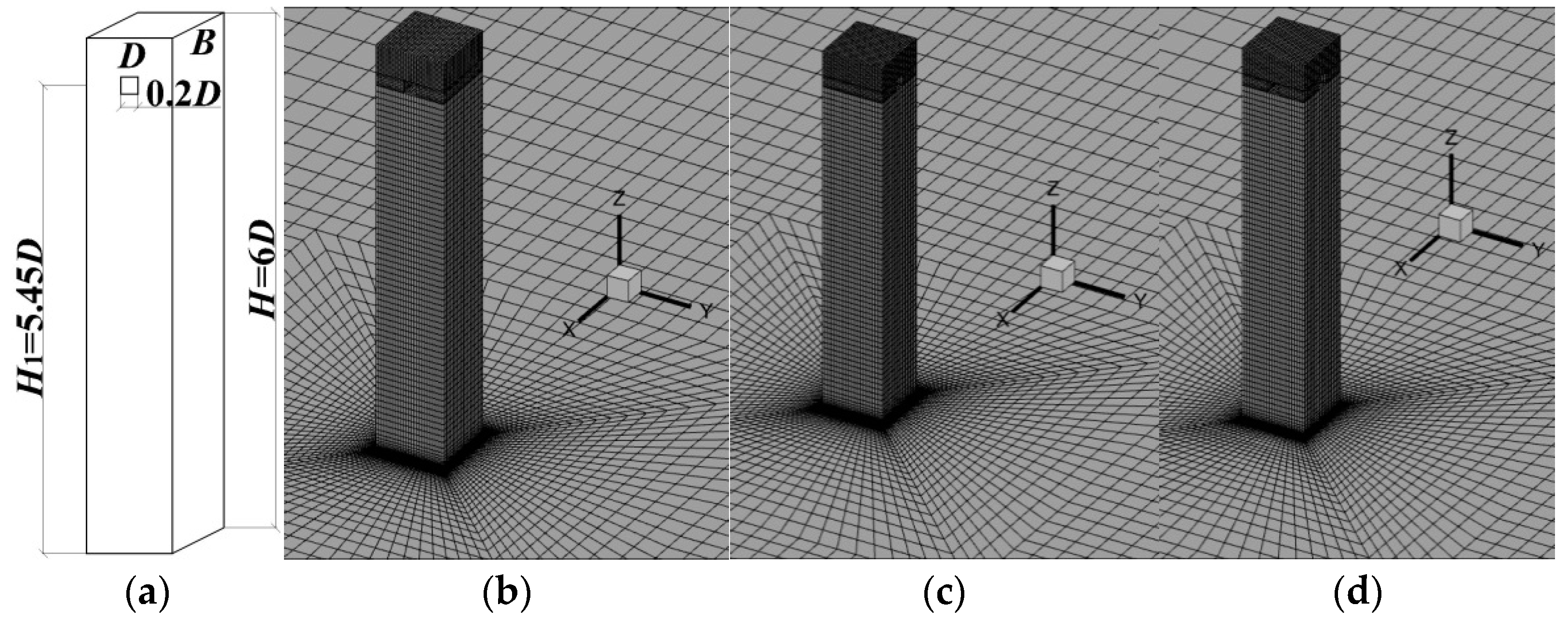
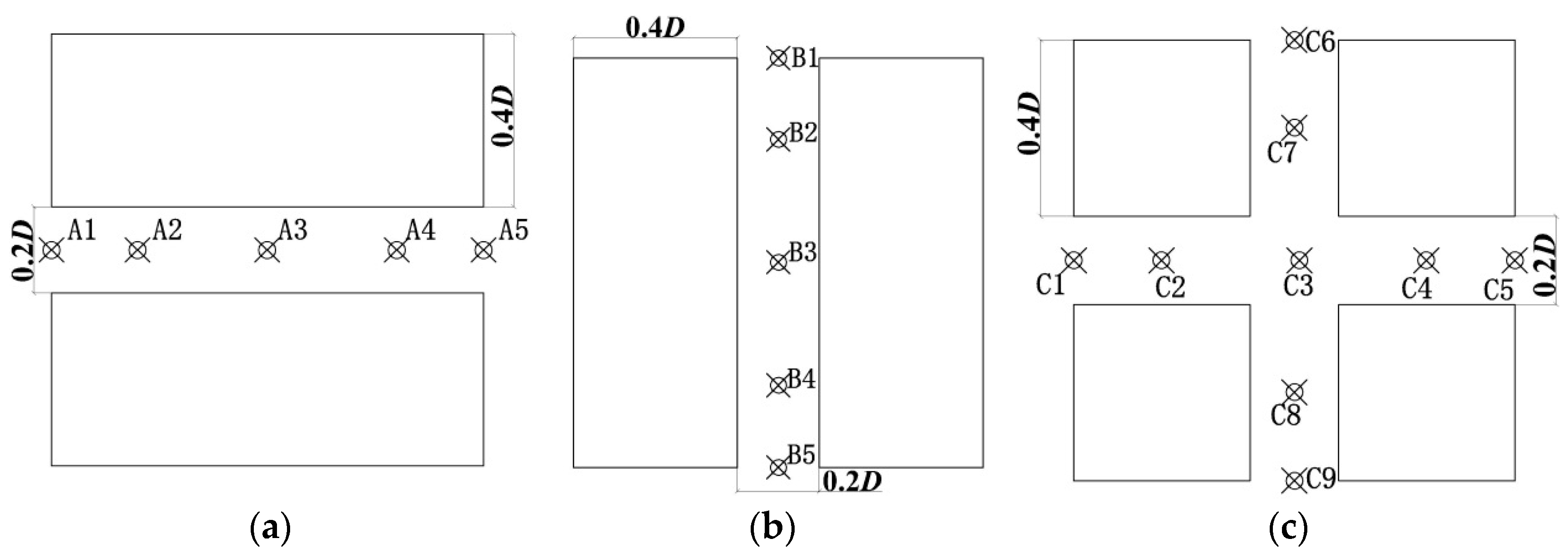
To compare with existing wind tunnel experiments, the scale ratio of the numerical simulation model in this study was consistent with that of the related literature [25]. A 1:500 scaled model of a high-rise building with a square section with a 1:6 aspect ratio of width to height and the length and width of D = B = 0.1 m was taken as the research object. The blockage ratio of the domain was 0.46%, thus meeting the blockage requirement [26]. The Reynolds number, which is based on building height H and incoming flow velocity UH at z = H, was 7.4 × 10⁴. The size of the computational domain was 94D(flow direction x) × 36D(spanwise direction y) × 36D(vertical direction z), as shown in Figure 2a. A structured grid was adopted for grid discretization, and the near-wall grid was appropriately encrypted, as shown in Figure 2b. Figure 2c shows a schematic diagram of the corresponding local encrypted area of the grid. Furthermore, to verify the effectiveness of the numerical simulation method and parameter settings, a square cylinder without opening measures was simulated via LES under different grid sizes, and the numerical simulation results were compared with those of the wind tunnel tests [25]. The three square cylinders with openings were named Case 1 (openings in X-direction), Case 2 (openings in Y-direction) and Case 3 (openings in both X-and Y-directions). The center of the opening hole was 5.45D away from the ground, as shown in Figure 3. Furthermore, Figure 4 illustrates the longitudinal section of the three models with openings. To study the effect of grid resolution, three different kinds of mesh schemes were arranged in the models, as shown in Table 1. The first grid point near the building model surface and the grid point near the ground were set to be different from each other. The grid stretch ratio was set to be less than 1.2, and the numbers of mesh schemes were about 8.96 × 10⁵ and 1.508 × 10⁶, respectively.

2.2. Boundary Conditions

To verify the effect of grid independence, the velocity inlet boundary conditions were determined by using the LES inflow pulsating method based on the self-sustaining boundary conditions. The incoming flow velocity is defined as follows:
u ( z ) = u K ln ( z + z 0 z 0 )
where the Von Karman constant K is 0.42, the roughness length z0 is 2.25 × 10⁻⁴ m, and the friction velocity u* is 0.557 m/s. The turbulent kinetic energy k(z) and dissipation rate ε(z) are determined as follows:
k ( z ) = 2 C 1 ln ( z + z 0 ) + C 2
ε = C μ 1 / 2 k ( z ) u z
where Cμ is a model constant, whose value is 0.09.
The basic idea of the LES method is to divide turbulence into large-scale and small-scale vortices. For large-scale vortices, the instantaneous N-S equation is directly solved, while for small-scale vortices, a model needs to be established to solve the equation. For a viscous incompressible fluid in the blunt-body flow problem, the governing equations after spatial averaging are as follows:
u i ¯ t = 0
u i ¯ t + u i ¯ u j ¯ x j = 1 ρ p ¯ x i + v 2 u i ¯ x j x j 1 ρ τ i j x i
where u i ¯ and u j ¯ are the velocity components and p ¯ is the pressure term after spatial averaging. τ i j = ρ u i u j ¯ ρ u i ¯ u j ¯ is the unclosed term that appears after the spatial averaging of the transient N-S equation, which is the momentum transport term between small-scale pulsations and large-scale vortices, reflecting the influence of the movement of small-scale vortices on the equation of motion that is being solved, which is called SGS subgrid stress. It is necessary to build a subgrid model to make the equations closed and solvable [27].
According to the subgrid model based on the vortex viscosity hypothesis proposed by Smagorinsky [28] and the Boussinesq hypothesis, the subgrid-scale stress can be obtained by using the following formula:
τ i j 1 3 τ k k δ i = 2 u t s ¯ i j
where u t is the subgrid turbulent viscosity coefficient; τ k k is the isotropic part of the subgrid stress, which is introduced into the filtered net pressure term to model it; and s ¯ i j is the solvable scale deformation rate tensor, which is determined as follows:
s ¯ i j = 1 2 ( u i ¯ x j + u i ¯ x i )
The differences among various subgrid models based on the vortex viscosity hypothesis are mainly reflected in the definition of subgrid turbulent viscosity coefficient [28].
In the Smagorinsky model, the viscosity coefficient of subgrid turbulence is defined as follows:
μ t = ρ L S 2 | S ¯ |
where LS is the subgrid-scale mixing length, and | S ¯ | = 2 S ¯ i j S ¯ i j . The subgrid mixing scale is defined as follows:
L S = min ( Κ d , C s V 1 / 3 )
where K is the von Karman constant; d is the distance near the wall; V is the volume of the calculation unit; and CS is the Smagorinsky constant, with its value varying according to the different properties of the flow field.
After further research and analysis of this problem by Germano [29] and Lilly [27], a dynamic value method, namely the dynamic Smagorinsky model, was determined, with a default value ranging from 0 to 0.23. Therefore, the dynamic Smagorinsky–Lilly model was chosen to be the subgrid model.
Firstly, the realizable k-ε turbulence model based on RANS was applied to calculate the steady flow around the square cylinder. The convergent flow field was taken as the initial flow field to carry out the spatial-averaged large eddy simulation. The SIMPLEC method was employed as the pressure–velocity coupling method, and the calculated residual was set to be 0.0005 [30]; the second-order implicit was used for the time discretization scheme and the time-step size was chosen to be 0.0005 s. The histograms in Figure 5 display the range of the cell Courant number of the three different mesh schemes, which show that more than 85% of the grid cells with three different grid sizes have a cell Courant number less than 1.0, indicating that the size of the time steps and meshes used in the present study basically meet the Courant–Friedrichs–Lewy (CFL) condition. The bounded central differencing scheme with second-order precision was used for spatial discretization. The computations were conducted with 8000 time steps, and the last 5000 time steps were used for collecting and averaging the obtained unsteady data.

3. Results and Discussions

In this study, the parameters of the simulated wind field were calibrated mainly based on the mean wind speed profiles, turbulence intensity profiles and wind pressure coefficients acting on the structural surface. The Strouhal numbers for several cases, which were calculated based on the overall lift coefficient and the incoming flow velocity UH at z = H, are shown in Table 1.
The dimensionless wind pressure coefficients can be calculated as follows:
C p i = p i / 0.5 ρ U H 2
where pi is the wind pressure at the measurement point i of the model; ρ = 1.225 kg/m3 is the air density; and UH is the incoming wind speed at the model height. For convenience of analysis, in the following analysis, Cpi,mean and Cpi,rms represent the mean and RMS wind pressure coefficients at the measurement point i, respectively.
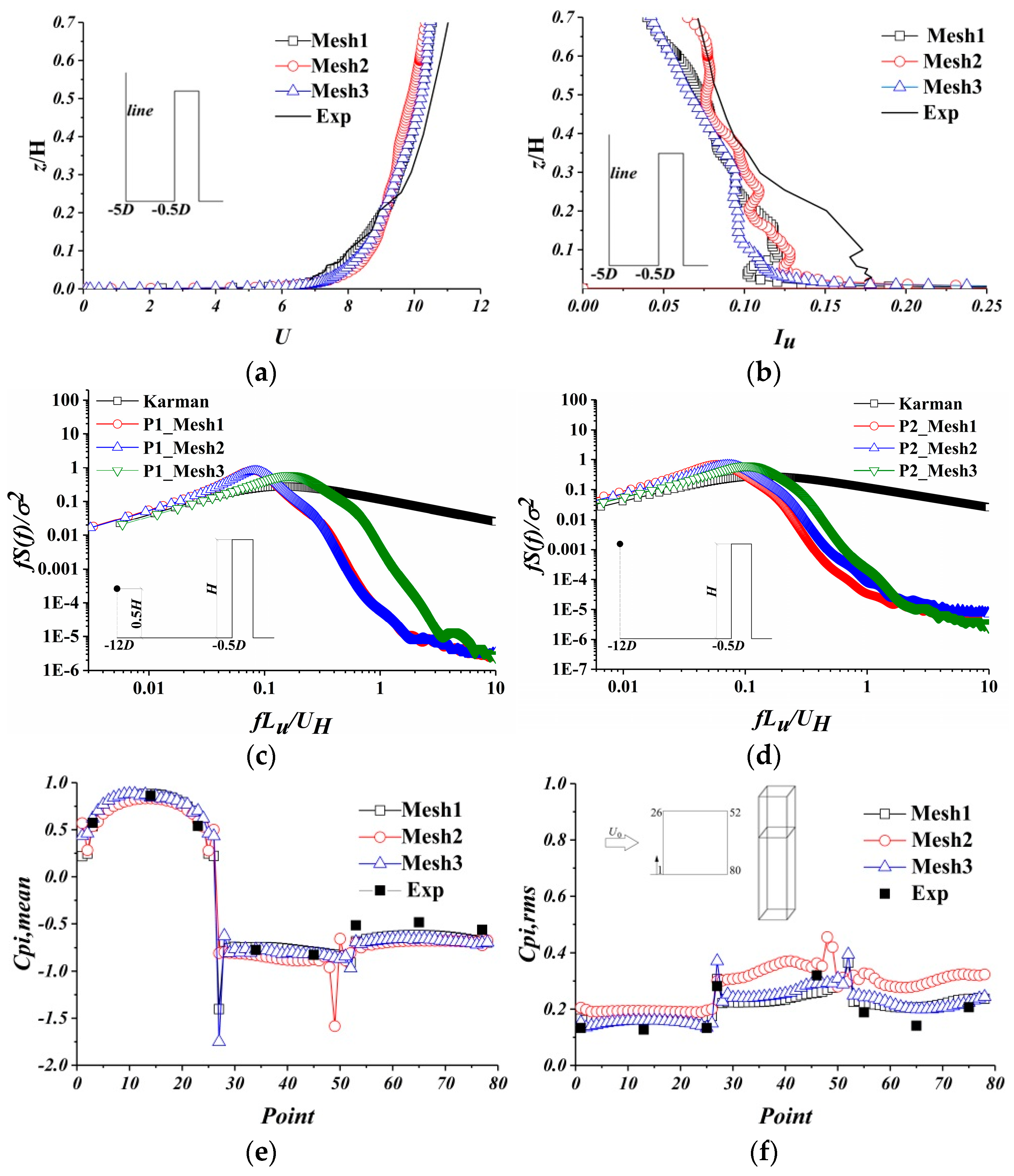
Figure 6 shows a comparison of the wind tunnel tests and numerical simulations. The wind tunnel test results were obtained from the literature [21]. Figure 6a,b show the comparisons of the simulated mean wind velocity and turbulence intensity of the points located at a height of 0.7H above the ground and 5D upstream from the windward side of the square cylinder, respectively. And the simulated wind velocity spectra of the points located at a height of 0.5H and H above the ground and 12D upstream from the windward side of the square cylinder are shown in Figure 6c,d, indicating that the wind velocity spectra obtained via LES could basically coincide with those of Karman at low frequencies, while there are decays in higher frequencies due to the filtering effect of the meshes. Then, the mean and RMS wind pressure coefficients of the standard cylinder at z = 2/3H were compared with the wind tunnel test results, and the results are shown in Figure 6e,f. The comparison indicated that (1) under the self-sustaining inflow boundary conditions, the mean wind velocity profiles are consistent with the wind tunnel test results. (2) In terms of turbulence, the simulated turbulence intensity profiles obtained via large eddy simulation are similar to the wind tunnel test results. Turbulence intensities decrease to a certain extent in the near-surface region, which is caused by ground friction. (3) For the three different near-wall grid sizes, the values of the wind pressure coefficients for the square cylinders are close to each other as a whole, and the variation trend is consistent with the test results. The mean wind pressure coefficients are in good agreement with the wind tunnel experiments. In terms of RMS wind pressures, the values are slightly higher than the wind tunnel test results on the windward and leeward sides. This is mainly caused by the oncoming turbulence on the windward side. In contrast, the Mesh 3 model with the minimum grid size of 0.0005D is more consistent with the experimental data. The grid sizes for the following cases were based on the Mesh 3 model.

3.1. Effect of Openings on Wind Speed Amplification of High-Rise Buildings

After establishing opening measures in high-rise buildings, the wind speed in the openings will be affected. In this study, monitoring points at different positions were set in the openings of Case 1, Case 2 and Case 3 to observe wind speed, and the results are shown in Figure 3. The wind speed amplification can be expressed as follows:
R i = U i / U r
where Ui is the mean wind speed at a measuring point in the openings, as shown in Figure 4, and Ur is the mean wind speed of the approaching location at the same height. Equation (11) reflects the variation in mean wind speed. To analyze the influence on the pulsating wind speed in the flow direction, the amplification of pulsating wind speed is defined by referring to the above equation:
R i , r m s = U i , r m s / U r
where Ui,rms is the RMS wind speed of the measuring point obtained via LES, as shown in Figure 4. From an observation of Table 2, it can be seen that after placing openings in the X-direction in the high-rise building, the mean and RMS wind speed in the openings both increased obviously compared to the wind speed of incoming flow at the same height (from A1 to A5). The wind speed amplification Ri in the openings presented a trend of first increasing and then decreasing, reaching a peak at the center of the cylinder. In Case 1, the mean wind speed amplification Ri of the monitoring points was basically the same as that for the RMS wind speed, which proves that in the case of along-wind openings in high-rise buildings, both the mean and RMS wind speed can increase in the openings, and the amplification amplitude Ri is relatively close. This is because the narrow tube effect caused by the along-wind openings causes an acceleration in the mean and RMS wind speed in the openings.
As can be observed in Table 3, for Case 2, the mean and RMS wind speed of the monitoring points decreased significantly compared with the incoming wind speed at the same height. Near the upper left side of the Y-direction openings, even reverse wind speed (B2) appeared. Compared to the mean wind speed, the RMS wind speed decreased slightly, but it was still much lower than the incoming wind speed, which was closely related to the shielding effect in the windward openings caused by the openings in the Y-direction in the high-rise building. Similarly, in Case 3 with openings in both X- and Y-directions, the wind speed at the monitoring points located at the downwind openings increased (C1–C5), especially at the central monitoring point C3 where the wind speed still presented an amplification even under the effect of openings in both X- and Y-directions. However, the wind speed at the four monitoring points in the across-wind openings still decreased significantly (C6–C9), and the wind direction of the wind speed at points C6 and C7 also reversed, indicating that for high-rise buildings with openings, the measures of openings in both X- and Y-directions will cause completely opposite effects on the changes in wind speed in the tunnel. This is mainly because opening measures change the aerodynamic configuration of high-rise buildings and changes the flow separation of incoming flow on the structural surface, thus affecting the wind load and wind speed of high-rise buildings, which is a typical aerodynamic optimization method.

3.2. Distribution of Mean Wind Pressure Coefficients

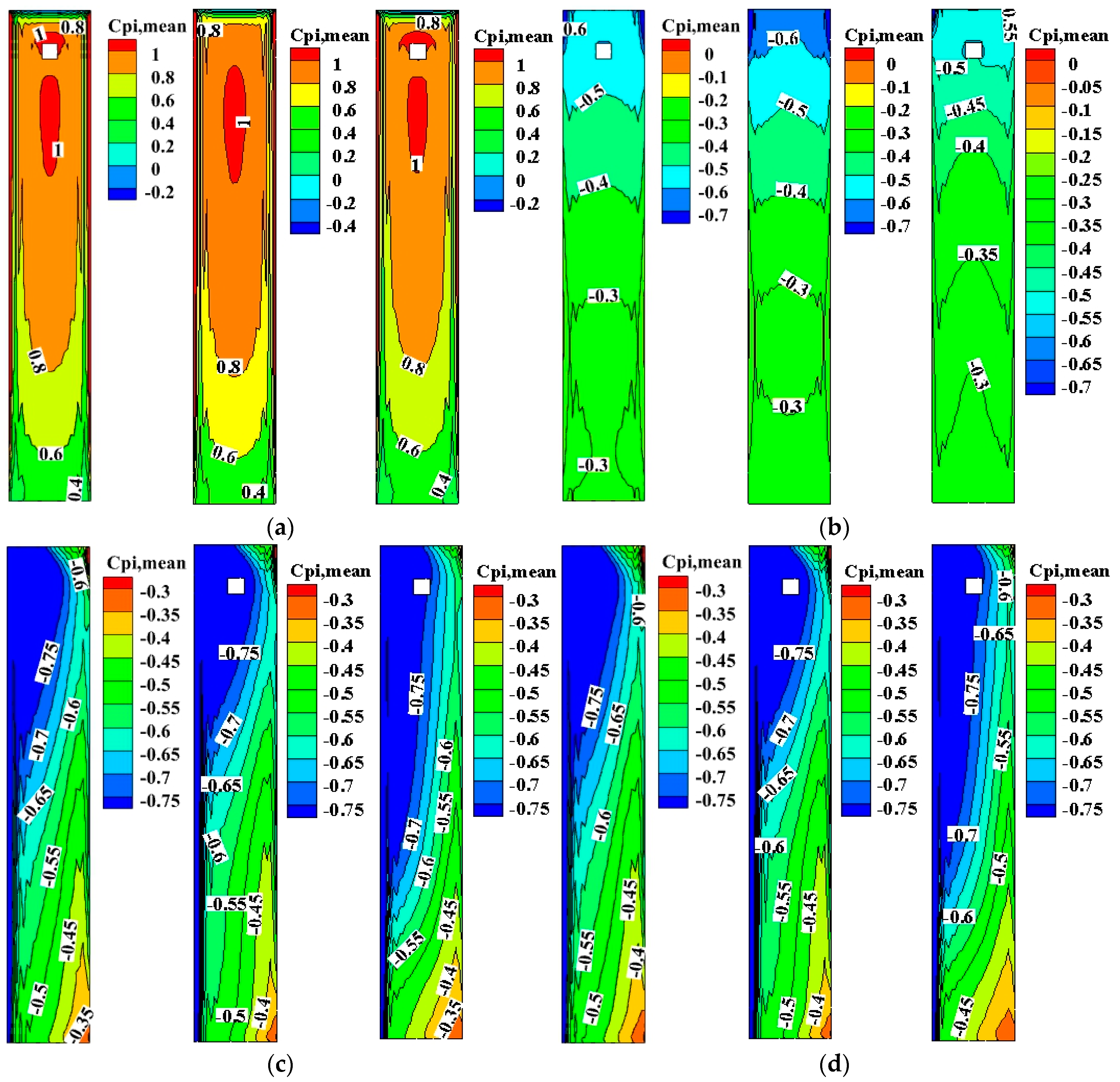
In this section, the contour clouds of the mean wind pressure coefficients on the surface for the standard square cylinder and the three types of opening models are presented to better understand the influence of different openings on high-rise buildings, which are shown in Figure 7 and Figure 8.
As it can be seen, the windward side of the standard cylinder is dominated by positive pressure, while the upper part of the windward side and leeward side is dominated by negative pressure, showing a symmetrical distribution. The wind speed of the incoming flow increases with an increase in height, which enhances the flow separation phenomenon. The mean value of the wind pressure coefficient increases with an increase in height above the ground on the windward and leeward sides. The mean wind pressure coefficients on the windward surfaces reach an extreme value on both sides and the upper area, but decrease somewhat at the top, which is caused by the three-dimensional flow effect of the building. The distribution of wind pressure on the left and right sides is basically the same, and the negative pressure reaches an extreme value on the leading edge, and then gradually decreases with the direction of incoming flow, with the minimum wind pressure at the top and bottom. After establishing opening measure, the incoming flow originally blocked by the building surface at the entrance directly passes through the entrance, resulting in a large change in wind pressure at the edge of the entrance due to flow separation, which mainly affects the distribution of wind pressure in the local areas of the entrance.
As can be seen from Figure 8, under the configuration of openings in the X-direction, Y-direction and both directions, the distribution of mean wind pressure on the surface of the three types of opening buildings is basically consistent with that of the standard square cylinder. The differences are mainly reflected in the locations of the openings. On the windward and leeward sides, the wind pressure around the X-direction opening position of Case 1 and Case 3 surges to a maximum value. The reason for the above difference in distribution is that the existence of the X-direction openings forms a narrow tube effect, which makes the wind speed inside the opening greater than the average wind speed of the incoming flow at equal height (See Table 2 and Table 4), and the airflow through the opening accelerates significantly. As a result, the surrounding openings of Case 1 and Case 3 show greater negative pressure. However, Case 2 with Y-direction openings does not show this phenomenon at the same position, and the distribution of wind pressure is basically consistent with the standard square cylinder. On the left and right sides, the wind pressure of the three opening models is close to each other, showing negative pressure. However, in Case 2 and Case 3 openings, there is no significant wind pressure variation as observed in the X-direction openings. The mean wind pressure on the surface of the three models does not change significantly compared to the standard square cylinder. This indicates that the three opening measures considered have no obvious effect on weakening the overall mean wind pressure of the building. The X-direction openings can significantly alter the distribution of wind pressure in the area near the entrance, leading to wind speed amplification.

3.3. Analysis of Time-Averaged Flow Field

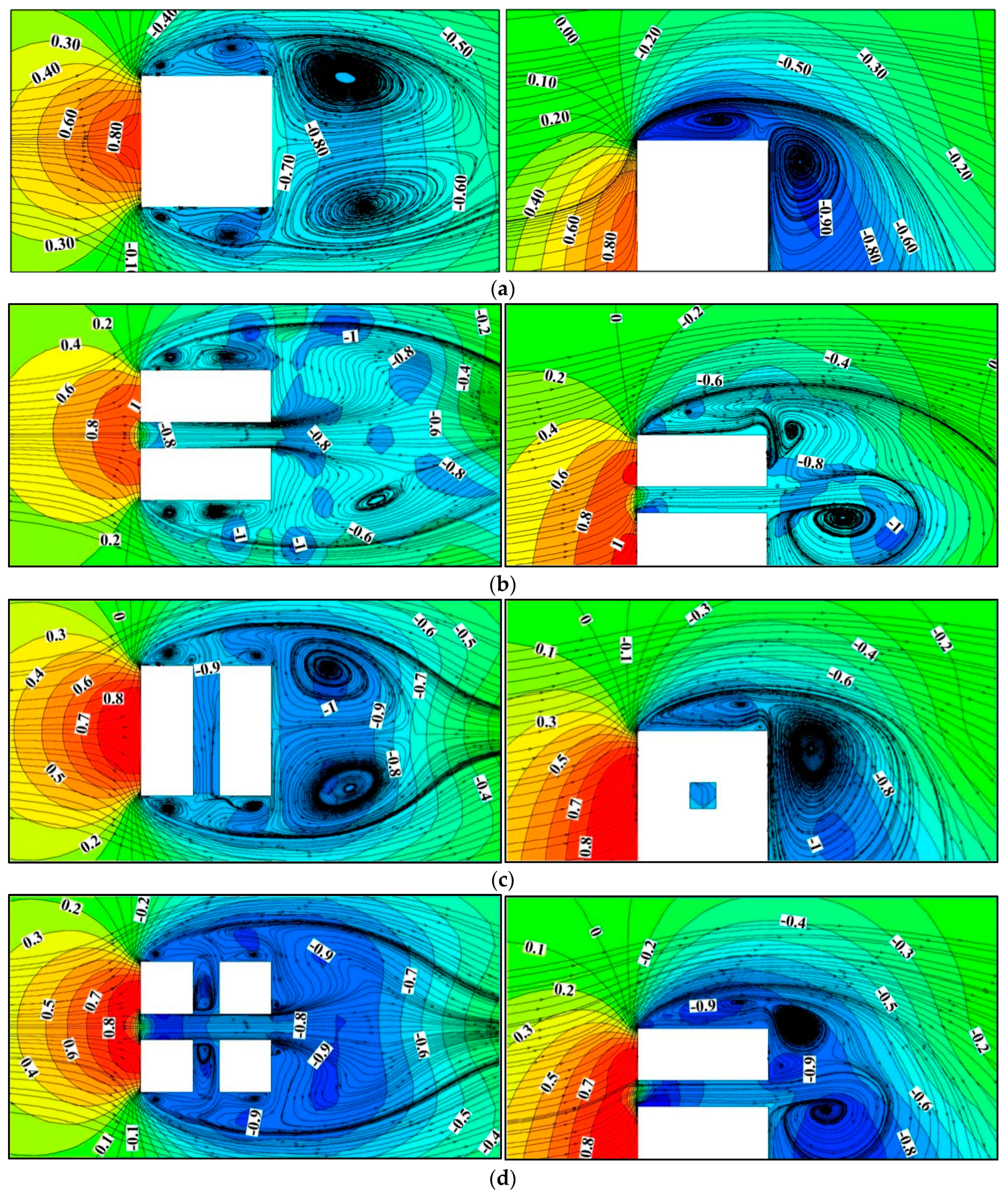
Compared to wind tunnel experiments, CFD numerical simulations have a great advantage in visualization of the flow field, which provides a basis for mechanism analysis. Compared to the RANS method based on time average, the LES method based on spatial average can obtain more comprehensive flow field information, including large-scale average flow and small-scale transient flow. Therefore, the influence mechanism of openings on wind load and wind speed amplification in high-rise buildings was analyzed from the perspective of flow field via LES. Figure 9 shows the time-averaged streamlines of the three opening models at the height of z = 0.55D and compares them with the time-averaged flow field of the standard square cylinder. The following conclusions can be drawn:
(1)
In general, one large-size separation vortex and two small-size separation vortices are formed on each side of the standard square cylinder close to the sidewall, and a pair of symmetric vortices of equal size and in opposite direction also exist on the leeward side. The large-size separation vortices and the small-size separation vortices at the upstream corner are connected with the leeward separation vortices. In the longitudinal section, the top of the windward side and the top of the leeward side of the square cylinder are separation points, and flow separation occurs when the air flows through this region. The top of the standard square cylinder and the top of the leeward surface each form a separate vortex, and the two separate vortices exist independently of each other. Due to the shielding effect of the structure, the incoming flow directly acts on the windward side of the structure, and then flow separation occurs at the top and two sides of the windward surface. Therefore, the side face and the top of the structure are in the separation zone. The suction effect is generated by the existence of the separation vortex, resulting in negative pressure on the side face and the top of the structure. The leeward side of the structure is subjected to the mixed effect of the separation vortex on the side face of the structure and the shedding vortex on the top, which produces wind suction, so it is also represented as negative pressure.
(2)
When compared with the standard square cylinder, the overall wind pressure distribution on the surface of the three opening models is consistent with the standard square cylinder, showing positive pressure on the windward side and negative pressure on the top, side face and leeward side. However, the wind pressure coefficient at the same position is different. For instance, the flow field around Case 1 changes significantly due to the aerodynamic measures of the X-direction openings. The wind pressure on the windward side is lower and the separation vortices behind the sidewalls of the cylinder are reattached on the flow field of the cross section. Symmetric vortices no longer appear on the leeward side. The incoming flow flows along with the openings, dividing the section into two rectangular sections with a large side ratio. The incoming flow in the openings disperses the large-scale separation vortices on the leeward side, and the generated separation vortices form vortices on the leeward side at the top of the tunnel. The scale of the generated separation vortices is lower than that of the standard square cylinder. The height of the vortex core is equal to the height of the tunnel, which reduces the negative pressure on the leeward side. Therefore, according to the cloud chart of wind pressure coefficient, the wind pressure difference between this area and the entrance of the opening on the windward side forms a narrow tube effect, which leads to a sharp increase in incoming wind speed in the opening due to the opening measure in the X-direction.
(3)
Similar to Case 1, the surrounding flow field and wind pressure distribution of Case 2 and Case 3 are clearly different from those of the standard square cylinder due to the opening measures. Under the opening measure in the Y-direction, due to the shielding effect of the windward side, the incoming flow in these openings basically has a lateral effect, and there is no large pressure difference due to the symmetrical distribution of wind pressure at both ends of the openings. As a result, although there is also a large negative pressure in the transverse openings, the X-direction wind speed in this area is significantly lower than that in the X-direction openings at the same height. After the measures for openings in both the X- and Y-directions are taken, the flow field and surface wind pressure distribution around Case 3 are close to those of Case 1. The wind speed under the influence of the measures of openings in both the X- and Y-directions presents an amplification compared to the wind speed of incoming flow at the same height (See Table 4). The wind speed amplification degree is slightly lower than that of Case 1, which also proves that the measure of X-direction openings plays a more important role in the incoming wind speed than that in the Y-direction.

3.4. Analysis of Instantaneous Flow Field

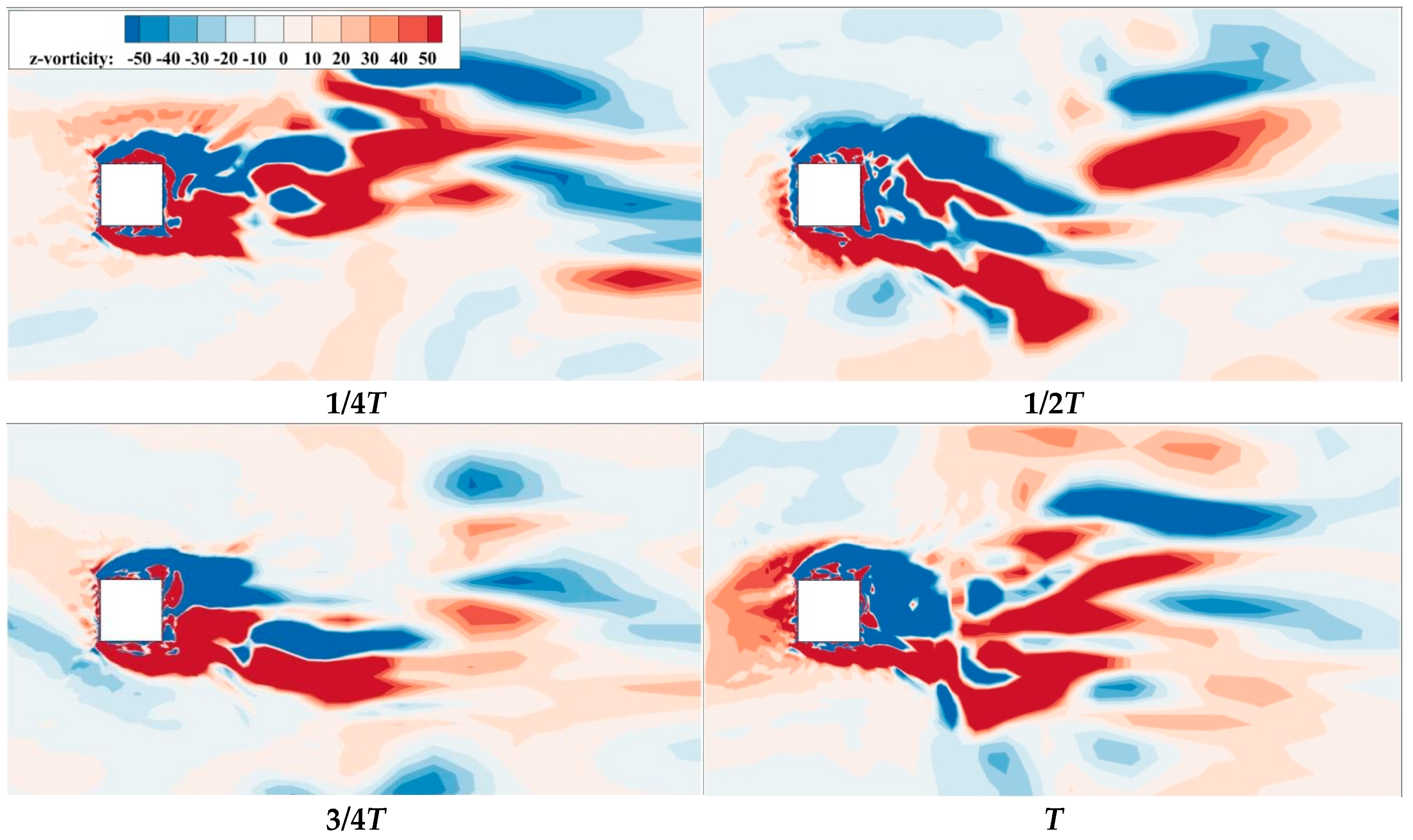
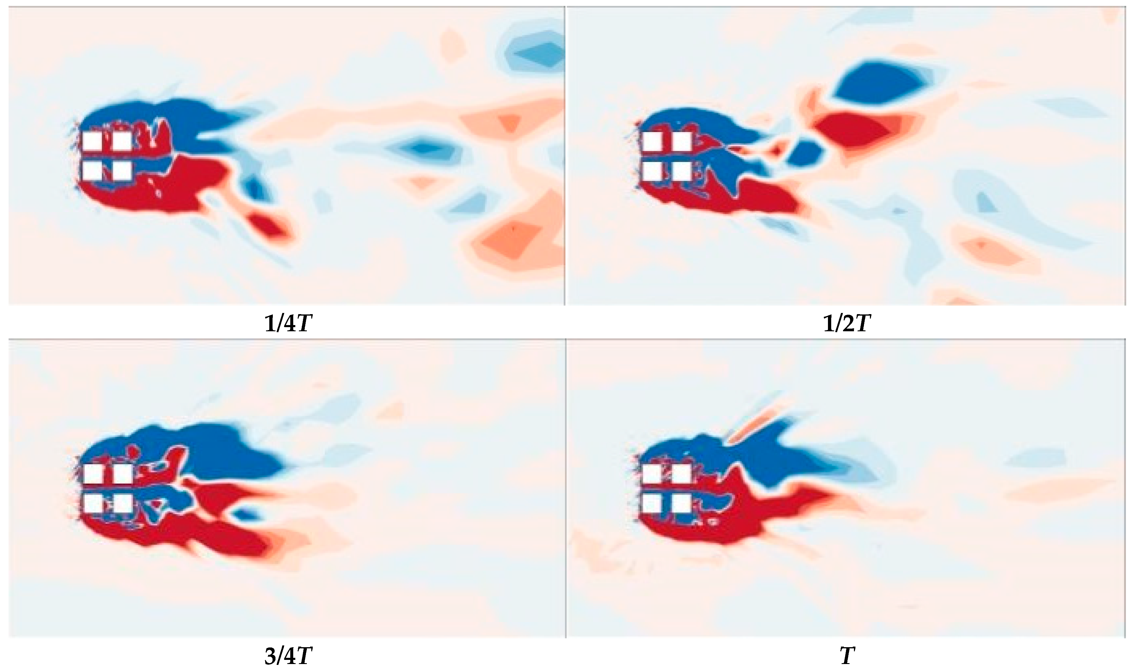
Figure 10 shows the distribution of instantaneous vortices at a section of the standard square cylinder model at four different moments within a certain period. It can be seen that there are abundant vortex structures around the standard square cylinder, with positive and negative vortices concentrated on the upper and lower sides of the cylinder, respectively. At different moments of the period, the shape of the surrounding vortices is also different. The positive vortices on the lower side are far away from the wall, while the negative vortices on the upper side are close to the wall. The vortex structure achieves flow separation on the windward side of the square cylinder, and gradually develops downstream over time. Finally, it reacts with the tail vortex on the leeward side and forms an alternating shedding trend of positive and negative vortices in the wake region.
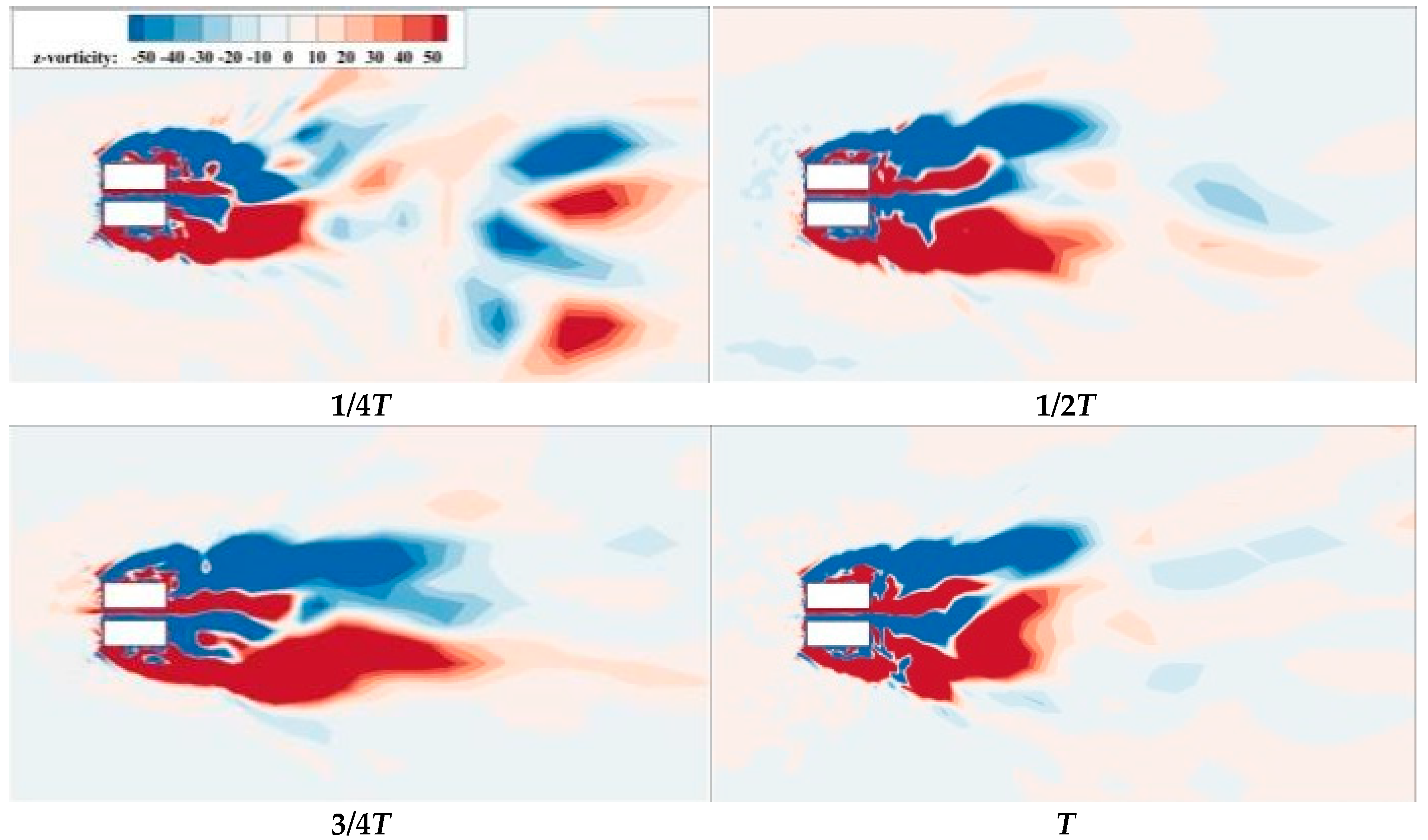
Figure 11, Figure 12 and Figure 13 show the distribution of instantaneous vortices for the three opening models at four classical moments. It can be seen that the instantaneous vortices of the three opening models are similar to those of the standard square cylinder. All of them achieve flow separation in the vortex structure on the windward side of the square cylinder. Compared to the three opening models, the scale of the tail vortex is smaller. In addition to the large-scale main vortex, more abundant smaller-scale vortices are formed, the vortex devolution frequency components are more complex, and the energy distribution is more dispersed. As the air flows around the square cylinder, the phenomena of separation, re-attachment and shedding appear on the model wall surface, and the formation and development of vortices are clarified. The vortices in the wake area fall off one by one and form developing vortices. Due to the opening measure, there are also abundant vortex structures gathered in the openings. In Case 3, the vortex structure in the openings is more complex, the vortex departure frequency components are more complex, and the energy distribution is more dispersed due to openings in both the X- and Y-directions.
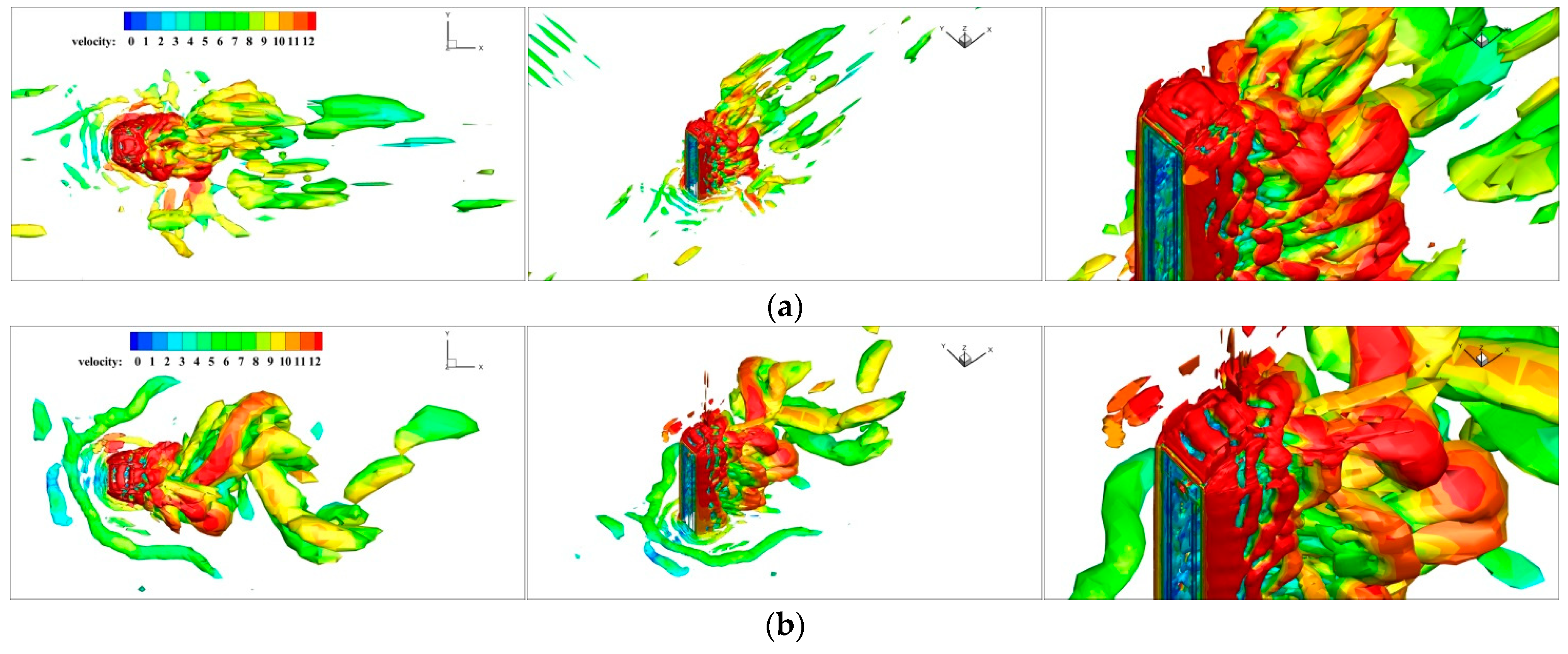
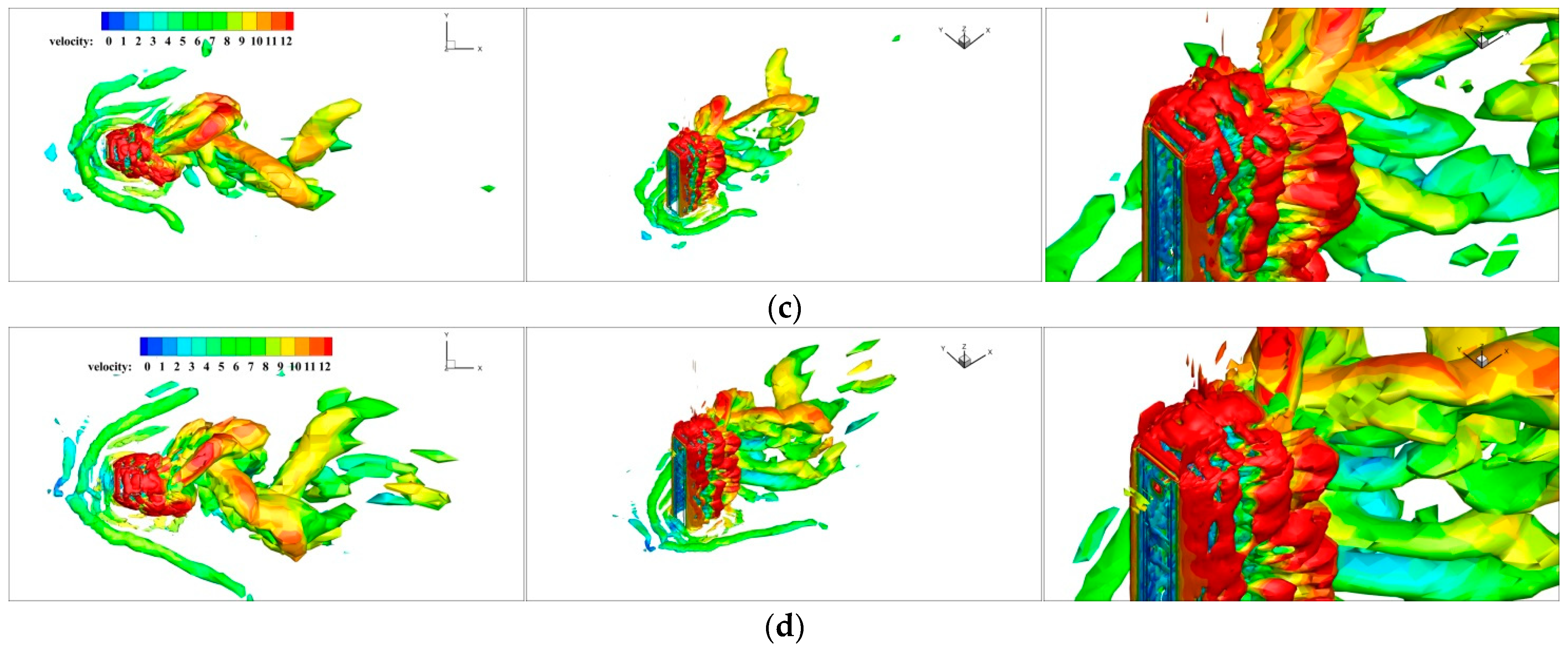
To obtain a better understanding of the distribution state of vortices in the whole flow field, as simulated by using LES, Figure 14 shows the three-dimensional structures of instantaneous vortices around the standard square cylinder and the three opening models at t = 4.0s when the value of the Q-criteria is 3000. In the figure, the vortex structures are presented with the flow direction and the wind speed. The following conclusions can be drawn:
(1)
A large number of vortex structures of different sizes and shapes are distributed around the structures. With a change in height, the vortex structures are also distributed differently, showing obvious three-dimensional characteristics. In the top region of the square cylinder, as the strip vortex separates at around the top separation point of the windward side of the upstream square cylinder, it mixes with the separation vortexes on both sides of the top, forming three-dimensional separation shear vortexes on the top of the square cylinder. With the continuous evolution of the vortex structure, the separation vortexes gradually move from the separation region to the downstream region. The measure of openings in the X-direction causes the flow separation point at the edge of the windward side to move down and the vortices at the top of the square cylinder to decrease. After establishing the openings in the X-direction, the narrow tube effect is formed, which not only accelerates the air flow through the entrance but also disorganizes the large-scale vortices on the leeward side. It forms several small-scale vortices near the entrance and on the leeward side, which disperses energy more. However, the measure of openings in the Y-direction leads to the lateral flow of separation vortices on both sides into the openings, which weakens the energy distribution on both sides. As a result, the lateral shear vortices of Case 2 are smaller than those of Case 1 and Case 3 and closer to the wall, which is determined by the variation in the aerodynamic configuration of the building caused by the opening measures.
(2)
Due to the friction effect on the ground, curved banded boundary-layer vortexes of different scales are generated in the near-ground region in front of the windward side for the three types of square cylinders with openings. The friction effect of the ground also causes the formation of spiral separation vortices on the side of the square cylinders, which is an embodiment of the turbulence pulsation of the incoming flow. Combined with the horizontal vortex diagrams in Figure 11, Figure 12 and Figure 13, the flow field morphology of Case 1, Case 2 and Case 3 is different after adopting openings in the X-direction, Y-direction and both X- and Y-directions, respectively. The side separation vortices of Case 2 are closer to the wall, and there are abundant small-scale vortices. In addition, three-dimensional strip separation vortices are also formed on the side of the square cylinder. The strip vortices of Case 1 and Case 3 have a larger scale and more concentrated vortex structure, while the strip vortices on the side of the square cylinder of Case 2 have a more dispersed scale. It can also be seen that the wind speed in the X-direction openings of Case 1 and Case 3 is significantly higher than that on the windward side of these square cylinders at the same height, while the windward side of Case 2 presents a lower wind speed as a whole due to the shielding effect. For vortices of various forms around the square cylinder, the larger these vortices are, the more energy they carry, the slower they move, and the smaller the wind pressure pulsation they generate. Conversely, the smaller the scale of the vortices, the more obvious the wind pressure pulsation. It is precisely because the opening measures change the aerodynamic configuration of the square cylinder that Case 1 and Case 3 gather small-scale vortex structures in the X-direction openings, which enhances the wind pressure pulsation and increases the mean and RMS wind speed in the openings, thus affecting the wind load on the surface of the square cylinder.

4. Conclusions

Three different opening measures for high-rise buildings were numerically simulated via LES in this study. The main conclusions can be summarized as follows:
(1)
The parameter settings and inflow turbulence based on self-sustaining boundary conditions and generated via LES were adopted. The simulated mean wind profiles and wind velocity spectra are basically consistent with the related wind tunnel test results and can well predict the wind loads of the square cylinders.
(2)
Under the effect of the opening measures, the aerodynamic configuration of the square cylinders is changed, and the wind load and incoming wind speed also vary. By adopting the X-direction opening measure, the pressure on the windward side of the square cylinders decreases. Part of the air flow in the square cylinders flows through the tunnel into the wake negative pressure area, which affects the flow separation point location, shear flow diffusion angle and flow reattachment phenomenon. Meanwhile, the wind speed in the openings increases significantly due to the narrow tube effect, which blows away the large-scale vortices on the leeward side, leading to energy dispersion and weakening the wind pressure on the structural surface. In contrast, the wind speed in the openings decreases significantly due to the shielding effect, and the wind load and the wind-induced response on the surface of the square cylinder are not significantly improved.
(3)
Under the measure of openings in both the X- and Y-directions, the vortex structures in the openings are more complex, the vortex departure frequency components are more complex, and the energy distribution is more dispersed. The wind speed in the X-direction openings still increases sharply, but the wind speed reduction in the Y-direction openings is weaker than that of Case 2. The wind speed in the central monitoring point still increases significantly under the influence of opening measures in both the X- and Y-directions, which proves that the X-direction openings play a more important role than the openings in the Y-direction.

Author Contributions

Conceptualization, F.C.; methodology, Y.L.; software, L.X.; validation, Y.Z.; formal analysis, Z.G.; investigation, Y.M.; resources, F.C.; data curation, Z.W.; writing—original draft preparation, Z.G.; writing—review and editing, Y.L.; visualization, L.X.; supervision F.C.; project administration, F.C.; funding acquisition, F.C. All authors have read and agreed to the published version of the manuscript.

Funding

This research was funded by the National Natural Science Foundation of China (Project No: 52278479), the Hunan Provincial Natural Science Foundation (Project No: 2023JJ30016), the Open Foundation of Key Laboratory of Safety and Control for Bridge Engineering of CSUST, Ministry of Education (Project No:13KB01), and the National Innovation and Entrepreneurship Training Program (Project No: 202210536010).

Institutional Review Board Statement

Not applicable.

Informed Consent Statement

Not applicable.

Data Availability Statement

The data presented in this study are available on request from the corresponding author. The data are not publicly available due to privacy.

Conflicts of Interest

The authors declare no conflict of interest.

References

  1. Li, J. Towards a low-carbon future in China’s building sector—A review of energy and climate models forecast. Energy Policy 2008, 36, 1736–1747. [Google Scholar] [CrossRef]
  2. Stathopoulos, T.; Alrawashdeh, H.; Al-Quraan, A.; Blocken, B.; Dilimulati, A.; Paraschivoiu, M.; Pilay, P. Urban wind energy: Some views on potential and challenges. J. Wind. Eng. Ind. Aerodyn. 2018, 179, 146–157. [Google Scholar] [CrossRef]
  3. Thellufsen, J.Z.; Lund, H.; Sorknæs, P.; Østergaard, P.A.; Chang, M.; Drysdale, D.; Nielsen, S.; Djørup, S.R.; Sperling, K. Smart energy cities in a 100% renewable energy context. Renew. Sustain. Energy Rev. 2020, 129, 109922. [Google Scholar] [CrossRef]
  4. Bagheri, M.; Delbari, S.H.; Pakzadmanesh, M.; Kennedy, C.A. City-integrated renewable energy design for low-carbon and climate-resilient communities. Appl. Energy 2019, 239, 1212–1225. [Google Scholar] [CrossRef]
  5. Stathopoulos, T. Computational wind engineering: Past achievements and future challenges. J. Wind. Eng. Ind. Aerodyn. 1997, 67–68, 509–532. [Google Scholar] [CrossRef]
  6. Tamura, T.; Itoh, Y.; Wada, A.; Kuwahara, K. Numerical study of pressure fluctuations on a rectangular cylinder in aerodynamic oscillation. J. Wind. Eng. Ind. Aerodyn. 1995, 54–55, 239–250. [Google Scholar] [CrossRef]
  7. Murakami, S.; Mochida, A.; Sakamoto, S. CFD analysis of wind-structure interaction for oscillating square cylinders. J. Wind. Eng. Ind. Aerodyn. 1997, 72, 33–46. [Google Scholar] [CrossRef]
  8. Larsen, A. Advances in aeroelastic analyses of suspension and cable-stayed bridges. J. Wind. Eng. Ind. Aerodyn. 1998, 74–76, 73–90. [Google Scholar] [CrossRef]
  9. Klemm, K.; Marks, W.; Klemm, A.J. Multicriteria optimisation of the building arrangement with application of numerical simulation. Build. Environ. 2000, 35, 537–544. [Google Scholar] [CrossRef]
  10. Hubbard, H.H.; Shepherd, K.P. Aeroacoustics of large wind turbines. J. Acoust. Soc. Am. 1991, 89, 2495–2508. [Google Scholar] [CrossRef]
  11. Bouffard, F.; Galiana, F.D. Stochastic Security for Operations Planning With Significant Wind Power Generation. IEEE Trans. Power Syst. 2008, 23, 306–316. [Google Scholar] [CrossRef]
  12. Hyams, M.A. Wind energy in the built environment. In Metropolitan Sustainability; Woodhead Publishing: Sawston, UK, 2012; pp. 457–499. [Google Scholar]
  13. Tamura, T.; Miyagi, T.; Kitagishi, T. Numerical prediction of unsteady pressures on a square cylinder with various corner shapes. J. Wind. Eng. Ind. Aerodyn. 1998, 74, 531–542. [Google Scholar] [CrossRef]
  14. Tamura, T.; Miyagi, T. The effect of turbulence on aerodynamic forces on a square cylinder with various corner shapes. J. Wind. Eng. Ind. Aerodyn. 1999, 83, 135–145. [Google Scholar] [CrossRef]
  15. Wang, X.R.; Gu, M. Experimental study on Re number effects on aerodynamic characteristics of 2D square prisms with corner modifications. Wind. Struct. 2016, 22, 573–594. [Google Scholar] [CrossRef]
  16. Risø, C. Urban Wind Energy-State of the Art 2009; National Laboratory for Sustainable Energy Technical University of Denmark: Roskilde, Denmark, 2009. [Google Scholar]
  17. Li, Q.S.; Chen, F.B.; Li, Y.G.; Lee, Y.Y. Implementing wind turbines in a tall building for power generation: A study of wind loads and wind speed amplifications. J. Wind. Eng. Ind. Aerodyn. 2013, 116, 70–82. [Google Scholar] [CrossRef]
  18. Li, Q.S.; Shu, Z.R.; Chen, F.B. Performance assessment of tall building-integrated wind turbines for power generation. Appl. Energy 2016, 165, 777–788. [Google Scholar] [CrossRef]
  19. Lu, C.L.; Li, Q.S.; Huang, S.H.; Zhao, S.L.; Zhu, C.N. Wind noise simulation and evaluation of a super high-rise building with wind turbine generators. J. Vib. Shock. 2012, 31, 5–9. (In Chinese) [Google Scholar]
  20. Chen, F.B.; Wang, X.L.; Zhao, Y.; Li, Y.B.; Li, Q.S.; Xiang, P.; Li, Y.; Mazzotti, C. Study of wind loads and wind speed amplifications on high-rise building with opening by numerical simulation and wind tunnel test. Adv. Civ. Eng. 2020, 2020, 8850688. [Google Scholar] [CrossRef]
  21. Ruiz, C.A.; Kalkman, I.; Blocken, B. Aerodynamic design optimization of ducted openings through high-rise buildings for wind energy harvesting. Build. Environ. 2021, 202, 108028. [Google Scholar] [CrossRef]
  22. Aristodemou, E.; Bentham, T.; Pain, C.; Colvile, R.; Robins, A.; ApSimon, H. A comparison of mesh-adaptive LES with wind tunnel data for flow past buildings: Mean flows and velocity fluctuations. Atmos. Environ. 2009, 43, 6238–6253. [Google Scholar] [CrossRef]
  23. Jiang, Y.; Alexander, D.; Jenkins, H.; Arthur, R.; Chen, Q. Natural ventilation in buildings: Measurement in a wind tunnel and numerical simulation with large-eddy simulation. J. Wind. Eng. Ind. Aerodyn. 2003, 91, 331–353. [Google Scholar] [CrossRef]
  24. Gousseau, P.; Blocken, B.; Stathopoulos, T.; Van Heijst, G.J.F. CFD simulation of near-field pollutant dispersion on a high-resolution grid: A case study by LES and RANS for a building group in downtown Montreal. Atmos. Environ. 2010, 45, 428–438. [Google Scholar] [CrossRef]
  25. Zheng, D.Q.; Zhang, A.S.; Gu, M. Improvement of inflow boundary condition in large eddy simulation of flow around tall building. Eng. Appl. Comput. Fluid Mech. 2012, 6, 633–647. [Google Scholar] [CrossRef]
  26. Baetke, F.; Werner, H.; Wengle, H. Numerical simulation of turbulent flow over surface-mounted obstacles with sharp edges and corners. J. Wind. Eng. Ind. Aerodyn. 1990, 35, 129–147. [Google Scholar] [CrossRef]
  27. Lilly, D.K. A proposed modification of the Germano subgrid-scale closure method. Phys. Fluids A Fluid Dyn. 1992, 4, 633–635. [Google Scholar] [CrossRef]
  28. Smagorinsky, J. General circulation experiments with the primitive equations. I. The basic experiment. Am. Meteorol. Soc. 1963, 91, 99–164. [Google Scholar]
  29. Germano, M.; Piomelli, U.; Moin, P.; Cabot, W.H. A dynamic subgrid-scale eddy viscosity model. Phys. Fluids 1998, 3, 1760–1765. [Google Scholar] [CrossRef]
  30. Doormaal, J.V.; Raithby, G.D. Enhancements of the simple method for predicting incompressible fluid flows. Numer. Heat Transf. Appl. 1984, 7, 147–163. [Google Scholar]
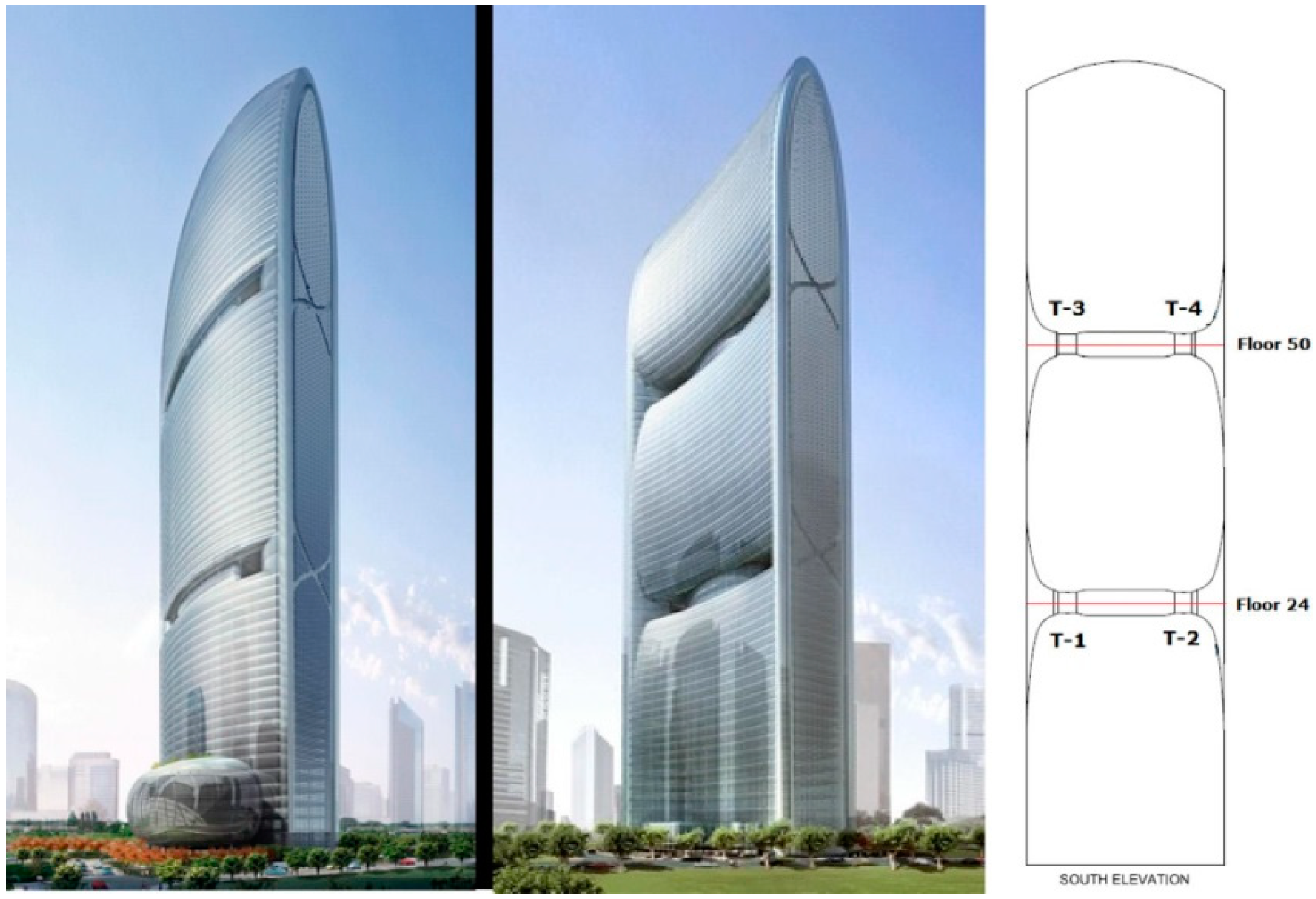
Figure 1. Overview of the Pearl River Tower [18].
Atmosphere 14 01687 g001
Figure 2. Computational situations: (a) computational domain and boundary conditions; (b) meshes for the whole domain; and (c) local meshes.
Atmosphere 14 01687 g002
Figure 3. Geometries and computational grids for three models with openings: (a) model without openings; (b) Case 1; (c) Case 2; and (d) Case 3.
Atmosphere 14 01687 g003
Figure 4. Longitudinal section of three models with openings: (a) Case 1; (b) Case 2; and (c) Case 3.
Atmosphere 14 01687 g004
Figure 5. Histograms of the range of CFL number of three mesh schemes: (a) Mesh 1; (b) Mesh 2; and (c) Mesh 3.
Atmosphere 14 01687 g005
Figure 6. Comparison of wind tunnel tests and numerical simulations: (a) mean wind velocity profile; (b) turbulence intensity profile and velocity spectrum at (c) z = 0.5H and (d) z = H; (e) mean wind pressure coefficients; and (f) RMS wind pressure coefficients.
Atmosphere 14 01687 g006
Figure 7. Mean wind pressure coefficients for standard cylinder: (a) windward; (b) leeward; (c) leftward; and (d) rightward.
Atmosphere 14 01687 g007
Figure 8. Comparison of mean pressure coefficients for three cases (from left to right: Case 1, Case 2 and Case 3): (a) windward; (b) leeward; (c) leftward; and (d) rightward.
Atmosphere 14 01687 g008
Figure 9. Comparison of time-averaged streamlines around the cylinder: (a) standard; (b) Case 1; (c) Case 2; and (d) Case 3.
Atmosphere 14 01687 g009
Figure 10. Standard square of distribution of instantaneous vortices.
Atmosphere 14 01687 g010
Figure 11. Distribution of instantaneous vortices in Case 1.
Atmosphere 14 01687 g011
Figure 12. Distribution of instantaneous vortices in Case 2.
Atmosphere 14 01687 g012aAtmosphere 14 01687 g012b
Figure 13. Distribution of instantaneous vortices in Case 3.
Atmosphere 14 01687 g013
Figure 14. Comparisons of the structure of transient vortices around the building model (from left to right: top view, overall view and partial enlarged view of top position): (a) standard; (b) Case 1; (c) Case 2; and (d) Case 3.
Atmosphere 14 01687 g014aAtmosphere 14 01687 g014b
Table 1. Case details for numerical simulation.
CaseMinimum Grid SizeStretch RatioNumber of Cellsy+St
Standard_Mesh 10.005D1.15896,000<300.098
Standard_Mesh 20.001D1.15896,000<150.096
Standard_Mesh 30.0005D1.101,508,000<50.098
Case 10.0005D1.101,540,000<50.092
Case 20.0005D1.101,540,000<50.09
Case 30.0005D1.101,400,000<50.092
Table 2. Model calculation conditions for Case 1.
A1A2A3A4A5
Ri1.0241.361.301.271.10
Ri,rms1.0251.361.311.281.11
Table 3. Model calculation conditions for Case 2.
B1B2B3B4B5
Ri0.0055−0.0010.001290.002550.0001
Ri,rms0.0770.0490.0490.0520.093
Table 4. Model calculation conditions for Case 3.
C1C2C3C4C5
Ri1.061.411.261.281.24
Ri,rms1.071.411.261.281.25
C6C7C8C9
Ri−0.022−0.003630.002480.028
Ri,rms0.070.0750.0750.078
Disclaimer/Publisher’s Note: The statements, opinions and data contained in all publications are solely those of the individual author(s) and contributor(s) and not of MDPI and/or the editor(s). MDPI and/or the editor(s) disclaim responsibility for any injury to people or property resulting from any ideas, methods, instructions or products referred to in the content.