
A Statistical Approach on Estimations of Climate Change Indices by Monthly Instead of Daily Data


Abstract
:1. Introduction
2. Method
2.1. Climate Change Indices
2.2. Applied Indices
2.3. Regression Functions
2.4. Methodological Approach
2.5. Used Data
3. Results
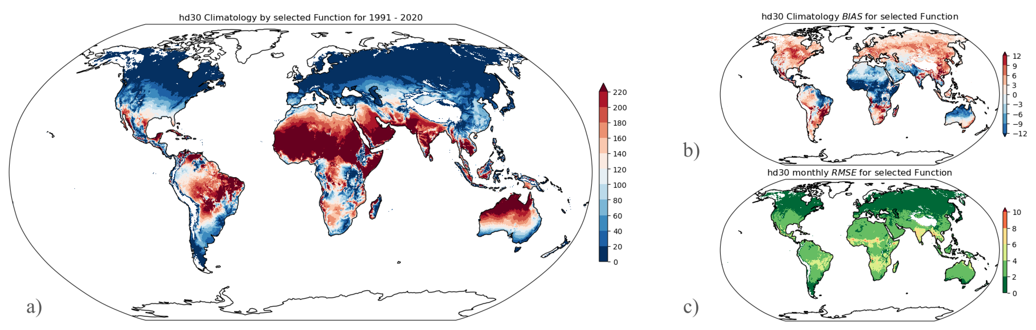
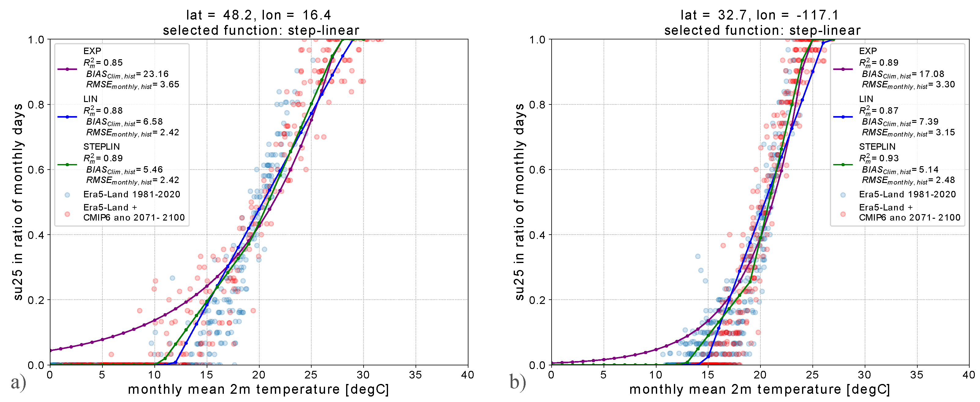
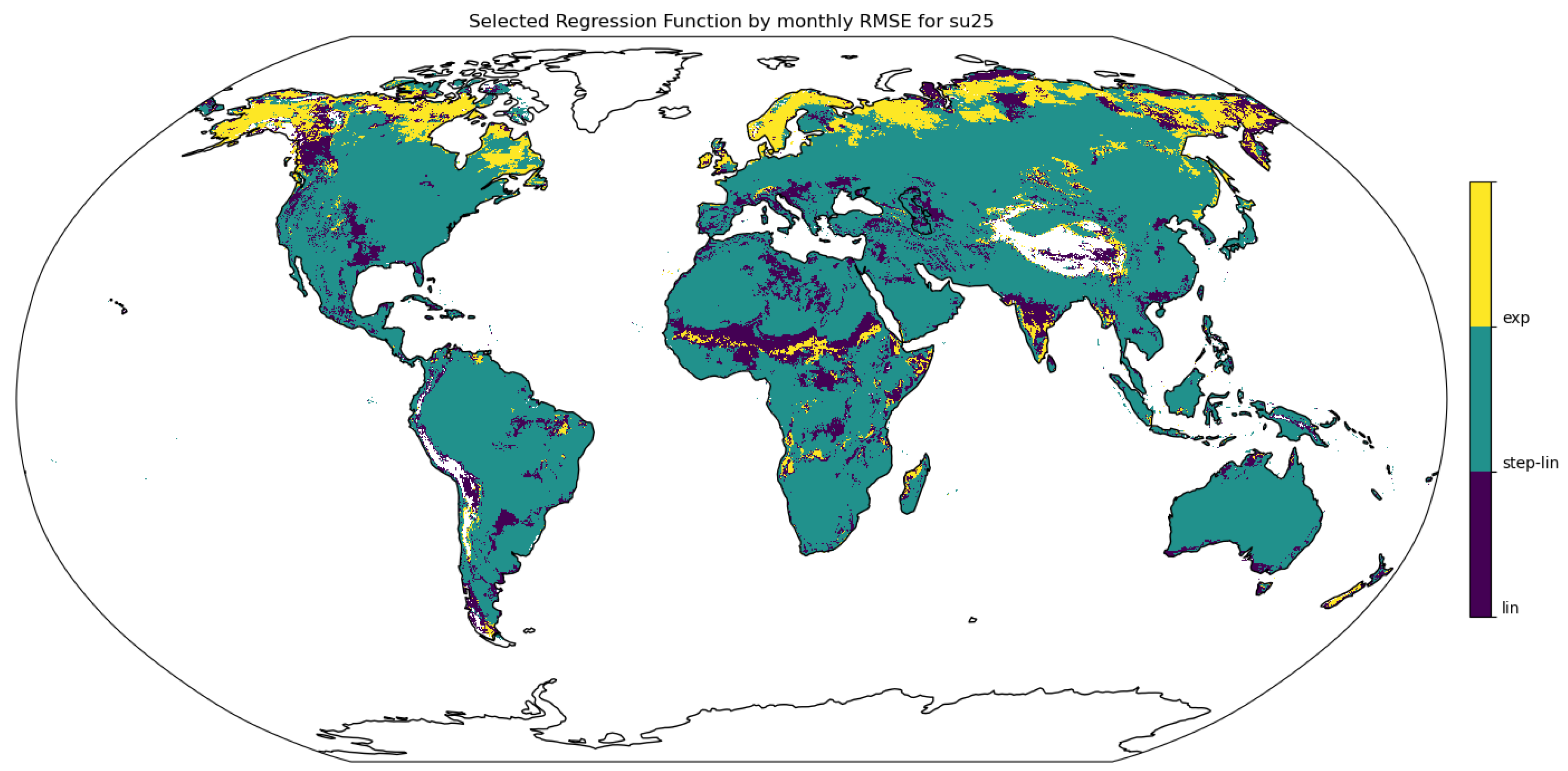
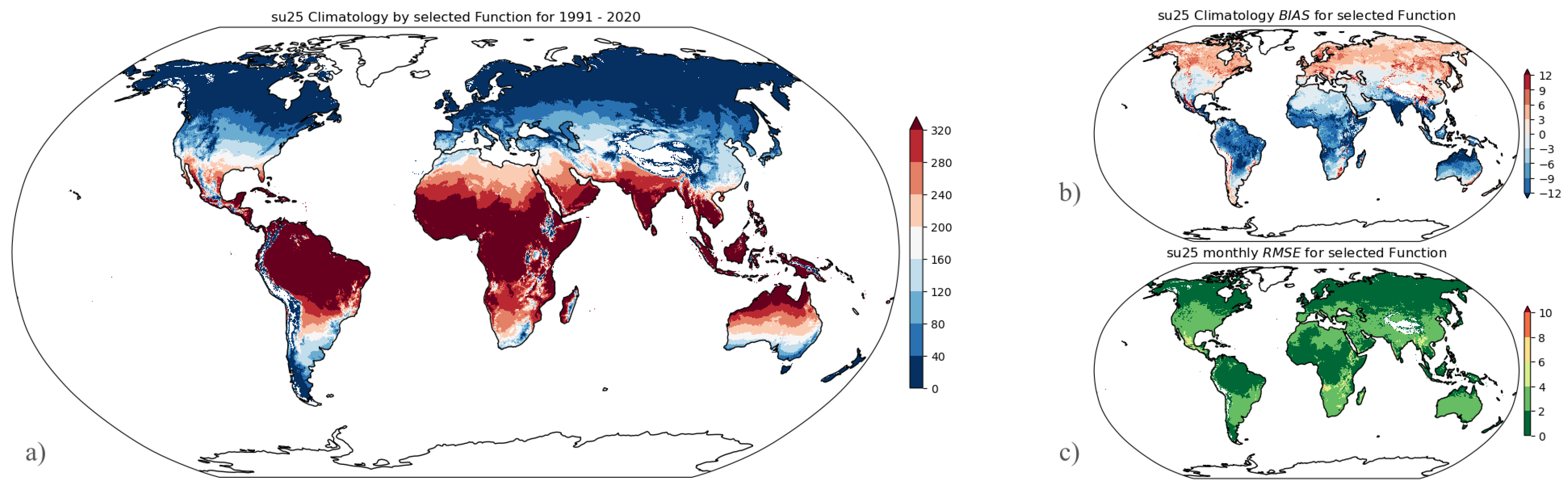
3.1. Summer Days
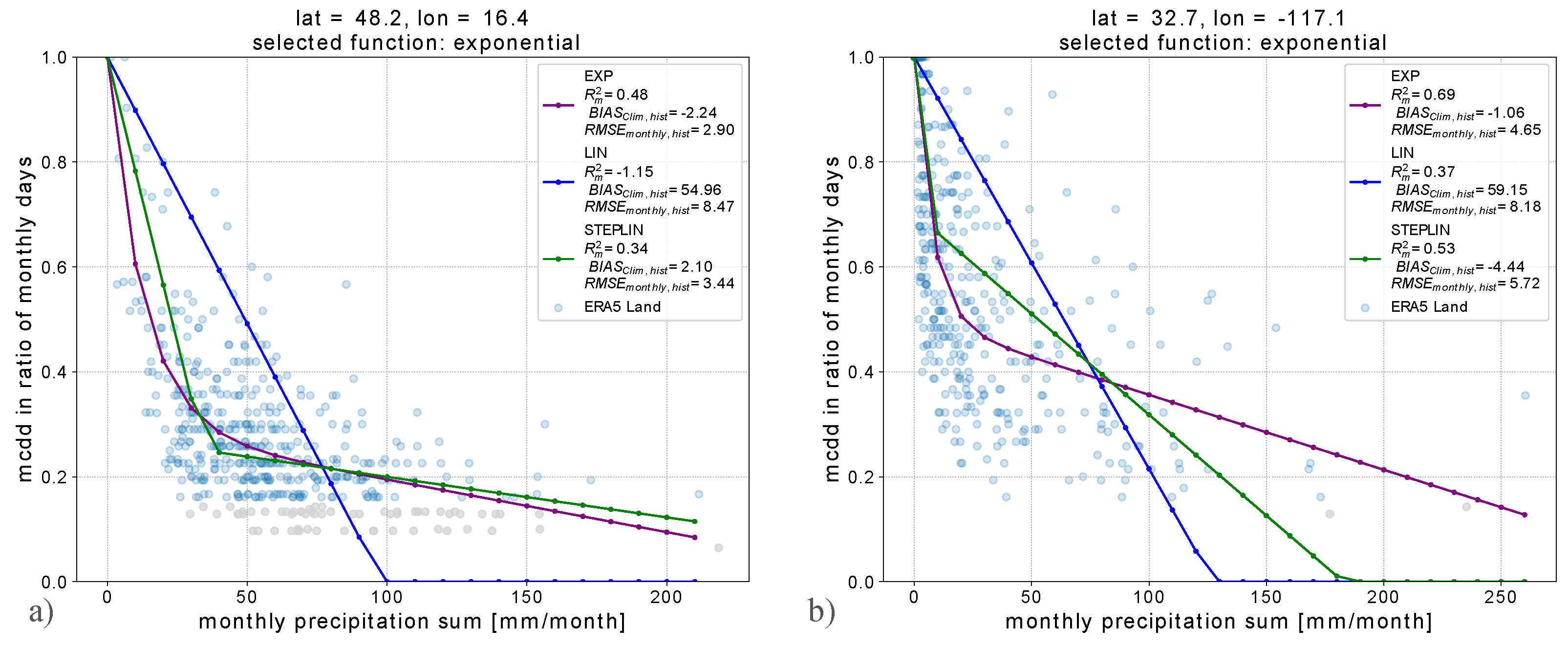
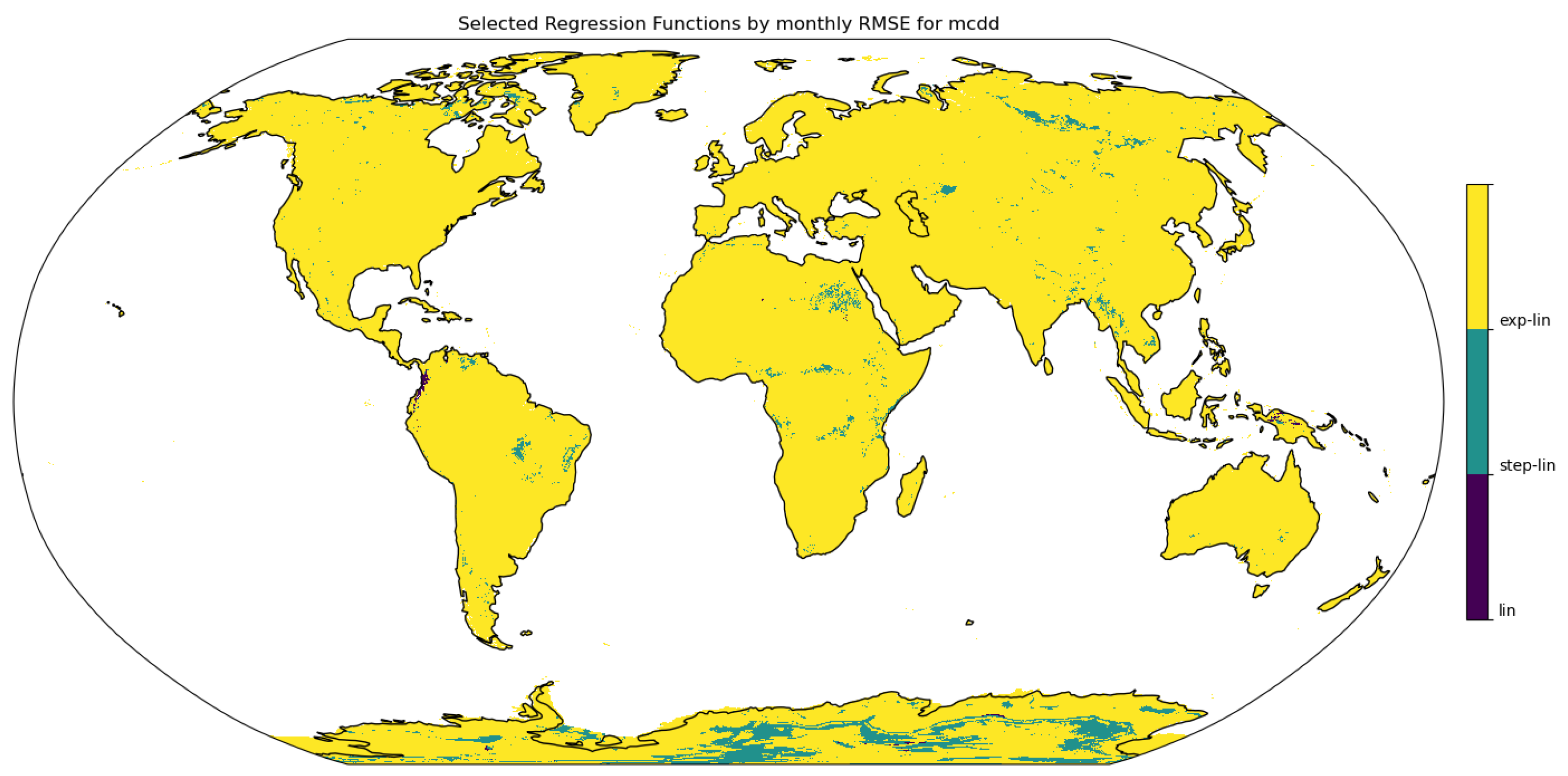
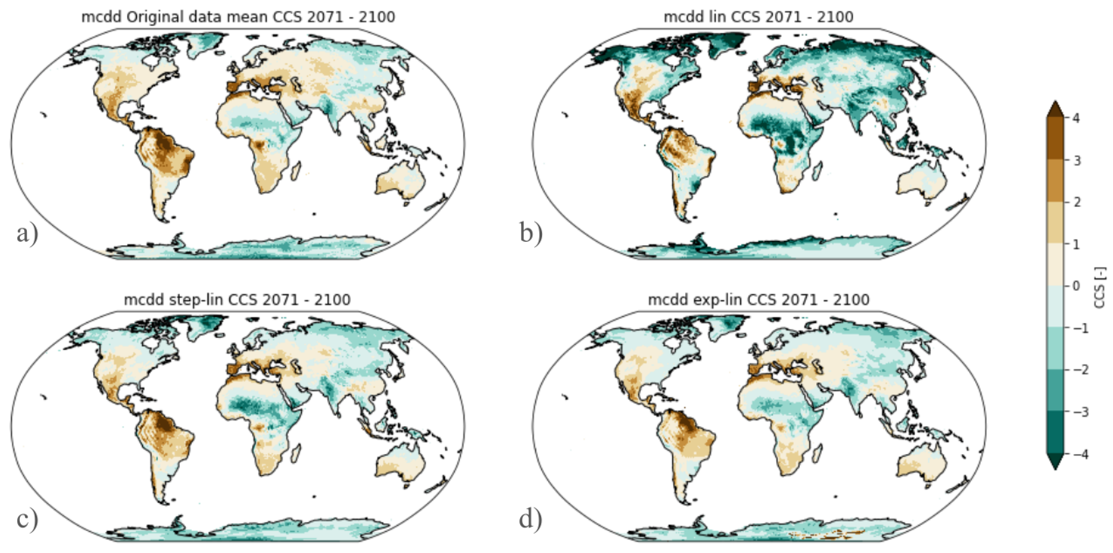
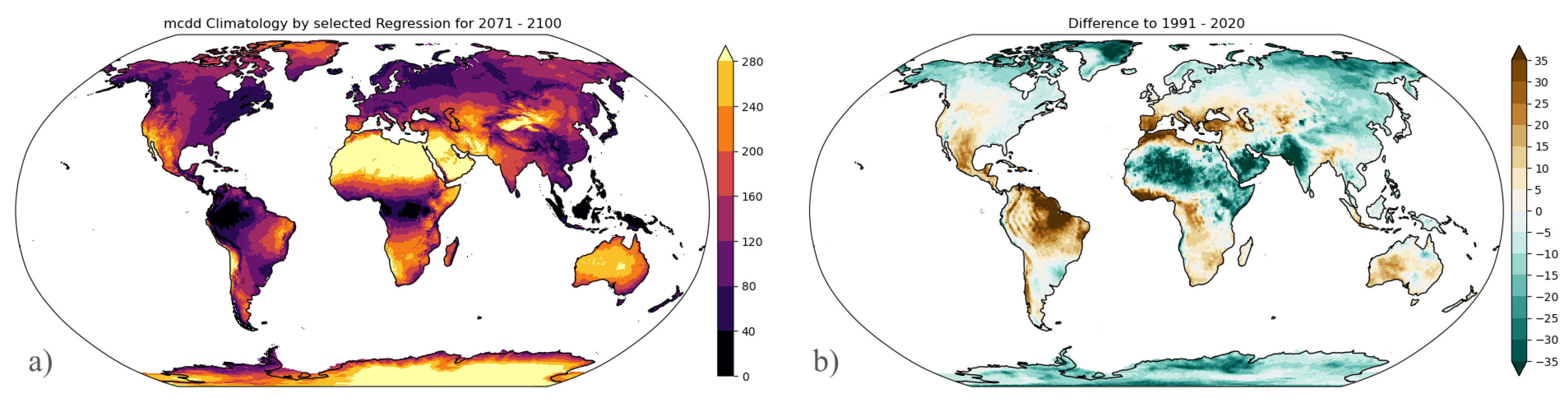
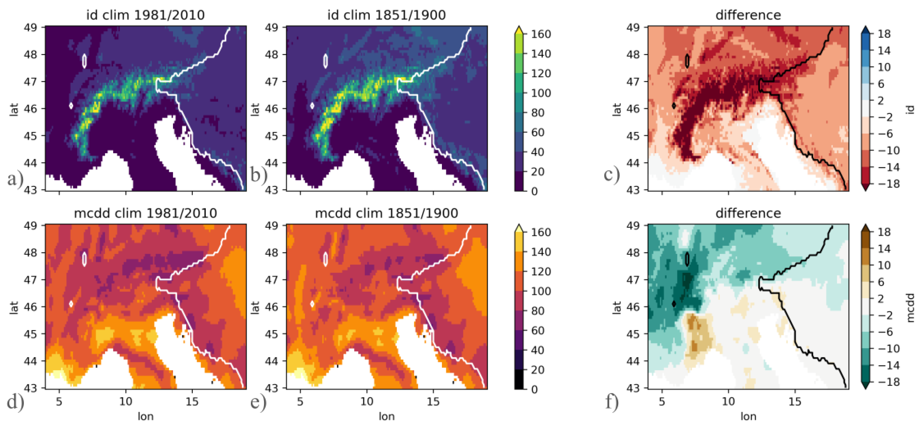
3.2. Maximum Consecutive Dry Days
3.3. Metrics by Updated Köppen–Geiger Climate Zones for Both Temperature and Precipitation Climate Change Indices
4. Examples of Use
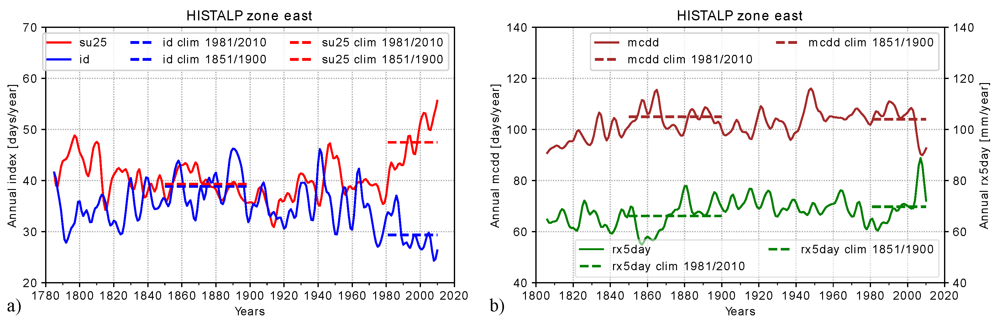
4.1. Calculation of CCI for HISTALP
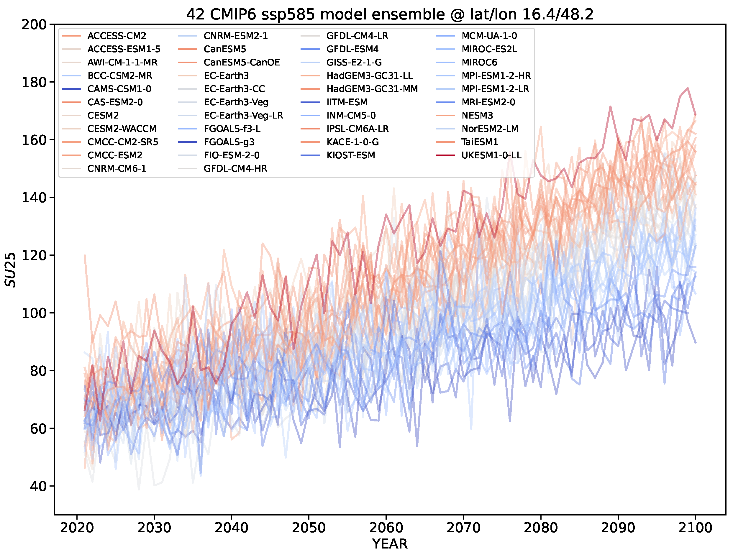
4.2. CMIP6 Ensemble Calculation
5. Discussion and Conclusions
Author Contributions
Funding
Institutional Review Board Statement
Data Availability Statement
Acknowledgments
Conflicts of Interest
Abbreviations
| CCI | Climate change index |
| CMIP6 | Coupled model intercomparison project 6 |
Appendix A
Appendix A.1. Impact of Including Consecutive Events below Five Days in the MCDD’s Climatology
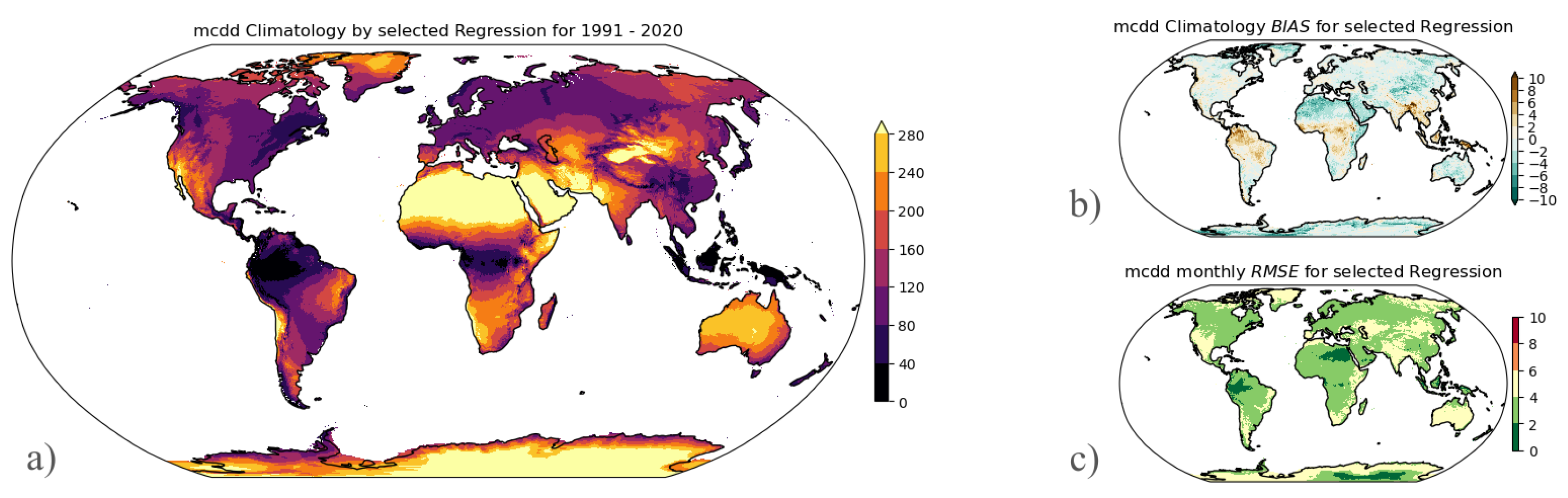

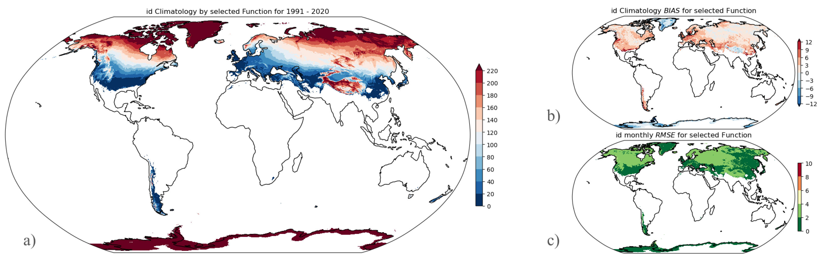
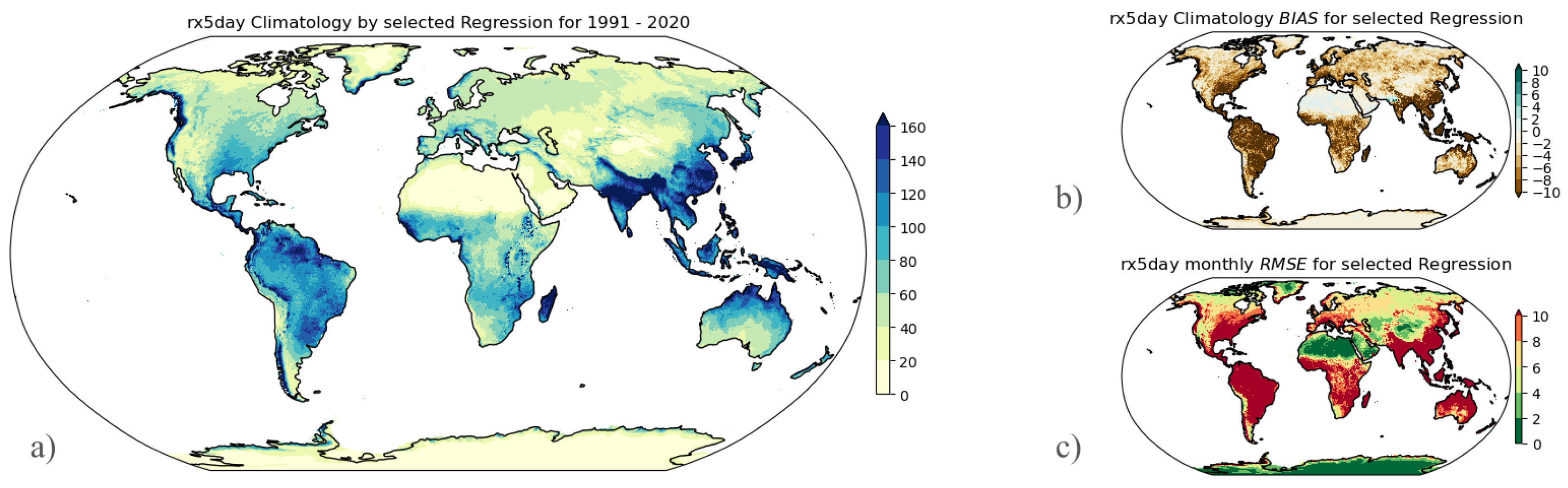
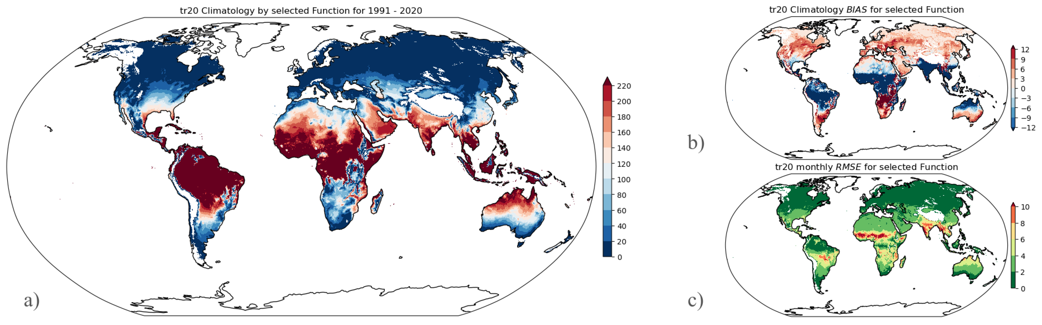
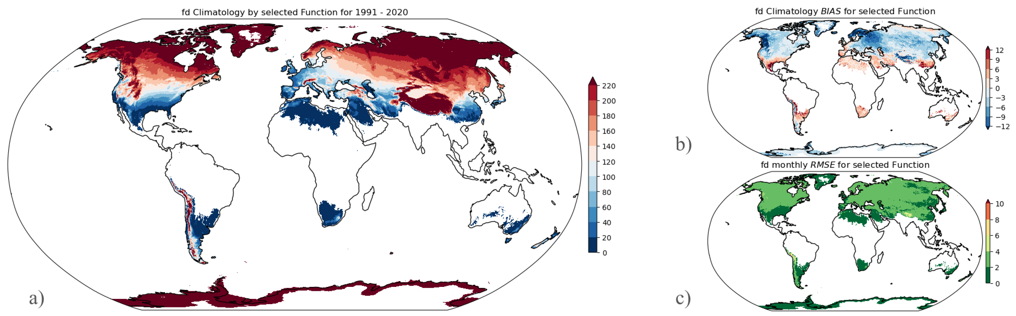
Appendix A.2. Climatology of Precipitation and Temperature Indices with BIAS and RMSE for the Period 1991 to 2020


References
- Geng, T.; Jia, F.; Cai, W.; Wu, L.; Gan, B.; Jing, Z.; Li, S.; McPhaden, M.J. Increased occurrences of consecutive La Niña events under global warming. Nature 2023, 619, 774–781. [Google Scholar] [CrossRef] [PubMed]
- Zachariah, M.; Philip, S.; Pinto, I.; Vahlberg, M.; Singh, R.; Otto, F.; Barnes, C.; Kimutai, J. Extreme Heat in North America, Europe and China in July 2023 Made Much More Likely by Climate Change; Grantham Institute for Climate Change: London, UK, 2023. [Google Scholar] [CrossRef]
- Sillmann, J.; Roeckner, E. Indices for extreme events in projections of anthropogenic climate change. Clim. Chang. 2008, 86, 83–104. [Google Scholar] [CrossRef]
- Mora, C.; Dousset, B.; Caldwell, I.R.; Powell, F.E.; Geronimo, R.C.; Bielecki, C.R.; Counsell, C.W.; Dietrich, B.S.; Johnston, E.T.; Louis, L.V.; et al. Global risk of deadly heat. Nat. Clim. Chang. 2017, 7, 501–506. [Google Scholar] [CrossRef]
- Lee, I.; Voogt, J.A.; Gillespie, T.J. Analysis and comparison of shading strategies to increase human thermal comfort in urban areas. Atmosphere 2018, 9, 91. [Google Scholar] [CrossRef]
- García Molinos, J.; Halpern, B.S.; Schoeman, D.S.; Brown, C.J.; Kiessling, W.; Moore, P.J.; Pandolfi, J.M.; Poloczanska, E.S.; Richardson, A.J.; Burrows, M.T. Climate velocity and the future global redistribution of marine biodiversity. Nat. Clim. Chang. 2016, 6, 83–88. [Google Scholar] [CrossRef]
- Zhao, C.; Liu, B.; Piao, S.; Wang, X.; Lobell, D.B.; Huang, Y.; Huang, M.; Yao, Y.; Bassu, S.; Ciais, P.; et al. Temperature increase reduces global yields of major crops in four independent estimates. Proc. Natl. Acad. Sci. USA 2017, 114, 9326–9331. [Google Scholar] [CrossRef]
- Jaegermeyr, J.; Müller, C.; Ruane, A.; Elliott, J.; Balkovic, J.; Castillo, O.; Faye, B.; Foster, I.; Folberth, C.; Franke, J.; et al. Climate change signal in global agriculture emerges earlier in new generation of climate and crop models. AGU Fall Meet. Abstr. 2021, 2021, U43D-06. [Google Scholar]
- Hirabayashi, Y.; Tanoue, M.; Sasaki, O.; Zhou, X.; Yamazaki, D. Global exposure to flooding from the new CMIP6 climate model projections. Sci. Rep. 2021, 11, 3740. [Google Scholar] [CrossRef]
- Droulia, F.; Charalampopoulos, I. Future climate change impacts on European viticulture: A review on recent scientific advances. Atmosphere 2021, 12, 495. [Google Scholar] [CrossRef]
- Alexander, L.V.; Arblaster, J.M. Assessing trends in observed and modelled climate extremes over Australia in relation to future projections. Int. J. Climatol. 2009, 29, 417–435. [Google Scholar] [CrossRef]
- Sillmann, J.; Kharin, V.; Zhang, X.; Zwiers, F.; Bronaugh, D. Climate extremes indices in the CMIP5 multimodel ensemble: Part 1. Model evaluation in the present climate. J. Geophys. Res. Atmos. 2013, 118, 1716–1733. [Google Scholar] [CrossRef]
- Formayer, H.; Nadeem, I.; Anders, I. Climate Change Scenario: From Climate Model Ensemble to Local Indicators. In Springer Climate; Springer: Cham, Switzerland, 2015; pp. 55–74. [Google Scholar] [CrossRef]
- Karl, T.R.; Nicholls, N.; Ghazi, A. Clivar/GCOS/WMO workshop on indices and indicators for climate extremes workshop summary. In Weather and Climate Extremes; Springer: Dordrecht, The Netherlands, 1999; pp. 3–7. [Google Scholar] [CrossRef]
- Peterson, T. Climate change indices. WMO Bull. 2005, 54, 83–86. [Google Scholar]
- Easterling, D.R.; Alexander, L.V.; Mokssit, A.; Detemmerman, V. CCI/CLIVAR workshop to develop priority climate indices. Bull. Am. Meteorol. Soc. 2003, 84, 1403–1407. [Google Scholar]
- Kharin, V.; Flato, G.; Zhang, X.; Gillett, N.; Zwiers, F.; Anderson, K. Risks from climate extremes change differently from 1.5 C to 2.0 C depending on rarity. Earth’s Future 2018, 6, 704–715. [Google Scholar] [CrossRef]
- Otto, F.E.; Massey, N.; van Oldenborgh, G.J.; Jones, R.G.; Allen, M.R. Reconciling two approaches to attribution of the 2010 Russian heat wave. Geophys. Res. Lett. 2012, 39. [Google Scholar] [CrossRef]
- Wartenburger, R.; Hirschi, M.; Donat, M.G.; Greve, P.; Pitman, A.J.; Seneviratne, S.I. Changes in regional climate extremes as a function of global mean temperature: An interactive plotting framework. Geosci. Model Dev. 2017, 10, 3609–3634. [Google Scholar] [CrossRef]
- Haylock, M.; Nicholls, N. Trends in extreme rainfall indices for an updated high quality data set for Australia, 1910–1998. Int. J. Climatol. 2000, 20, 1533–1541. [Google Scholar] [CrossRef]
- Frich, P.; Alexander, L.V.; Della-Marta, P.; Gleason, B.; Haylock, M.; Tank Klein, A.M.; Peterson, T. Observed coherent changes in climatic extremes during the second half of the twentieth century. Clim. Res. 2002, 19, 193–212. [Google Scholar] [CrossRef]
- Alexander, L.V.; Zhang, X.; Peterson, T.C.; Caesar, J.; Gleason, B.; Klein Tank, A.M.; Haylock, M.; Collins, D.; Trewin, B.; Rahimzadeh, F.; et al. Global observed changes in daily climate extremes of temperature and precipitation. J. Geophys. Res. Atmos. 2006, 111, D05109. [Google Scholar] [CrossRef]
- Cornes, R.C.; van der Schrier, G.; van den Besselaar, E.J.; Jones, P.D. An ensemble version of the E-OBS temperature and precipitation data sets. J. Geophys. Res. Atmos. 2018, 123, 9391–9409. [Google Scholar] [CrossRef]
- Jacob, D.; Petersen, J.; Eggert, B.; Alias, A.; Christensen, O.B.; Bouwer, L.M.; Braun, A.; Colette, A.; Déqué, M.; Georgievski, G.; et al. EURO-CORDEX: New high-resolution climate change projections for European impact research. Reg. Environ. Chang. 2014, 14, 563–578. [Google Scholar] [CrossRef]
- Keller, J.D.; Wahl, S. Representation of climate in reanalyses: An intercomparison for Europe and North America. J. Clim. 2021, 34, 1667–1684. [Google Scholar] [CrossRef]
- Megyeri-Korotaj, O.A.; Bán, B.; Suga, R.; Allaga-Zsebeházi, G.; Szépszó, G. Assessment of Climate Indices over the Carpathian Basin Based on ALADIN5. 2 and REMO2015 Regional Climate Model Simulations. Atmosphere 2023, 14, 448. [Google Scholar] [CrossRef]
- Lehtonen, I.; Ruosteenoja, K.; Jylhä, K. Projected changes in European extreme precipitation indices on the basis of global and regional climate model ensembles. Int. J. Climatol. 2014, 34, 1208–1222. [Google Scholar] [CrossRef]
- Dosio, A. Projections of climate change indices of temperature and precipitation from an ensemble of bias-adjusted high-resolution EURO-CORDEX regional climate models. J. Geophys. Res. 2016, 121, 5488–5511. [Google Scholar] [CrossRef]
- Viceto, C.; Cardoso Pereira, S.; Rocha, A. Climate change projections of extreme temperatures for the Iberian Peninsula. Atmosphere 2019, 10, 229. [Google Scholar] [CrossRef]
- Dikshit, A.; Pradhan, B.; Alamri, A.M. Temporal hydrological drought index forecasting for New South Wales, Australia using machine learning approaches. Atmosphere 2020, 11, 585. [Google Scholar] [CrossRef]
- Liu, J.; Liu, Y.; Chen, X.; Zhang, J.; Guan, T.; Wang, G.; Jin, J.; Zhang, Y.; Tang, L. Extreme Precipitation Events Variation and Projection in the Lancang-Mekong River Basin Based on CMIP6 Simulations. Atmosphere 2023, 14, 1350. [Google Scholar] [CrossRef]
- Auer, I.; Böhm, R.; Jurković, A.; Orlik, A.; Potzmann, R.; Schöner, W.; Ungersböck, M.; Brunetti, M.; Nanni, T.; Maugeri, M.; et al. A new instrumental precipitation dataset for the greater alpine region for the period 1800–2002. Int. J. Climatol. A J. R. Meteorol. Soc. 2005, 25, 139–166. [Google Scholar] [CrossRef]
- Auer, I.; Böhm, R.; Jurkovic, A.; Lipa, W.; Orlik, A.; Potzmann, R.; Schöner, W.; Ungersböck, M.; Matulla, C.; Briffa, K.; et al. HISTALP—Historical instrumental climatological surface time series of the Greater Alpine Region. Int. J. Climatol. A J. R. Meteorol. Soc. 2007, 27, 17–46. [Google Scholar] [CrossRef]
- Muñoz-Sabater, J.; Dutra, E.; Agustí-Panareda, A.; Albergel, C.; Arduini, G.; Balsamo, G.; Boussetta, S.; Choulga, M.; Harrigan, S.; Hersbach, H.; et al. ERA5-Land: A state-of-the-art global reanalysis dataset for land applications. Earth Syst. Sci. Data 2021, 13, 4349–4383. [Google Scholar] [CrossRef]
- O’Neill, B.C.; Tebaldi, C.; Van Vuuren, D.P.; Eyring, V.; Friedlingstein, P.; Hurtt, G.; Knutti, R.; Kriegler, E.; Lamarque, J.F.; Lowe, J.; et al. The Scenario Model Intercomparison Project (ScenarioMIP) for CMIP6. Geosci. Model Dev. 2016, 9, 3461–3482. [Google Scholar] [CrossRef]
- James, G.; Witten, D.; Hastie, T.; Tibshirani, R. An Introduction to Statistical Learning; Springer: New York, NY, USA, 2013; Volume 112. [Google Scholar]
- Jungclaus, J.; Bittner, M.; Wieners, K.H.; Wachsmann, F.; Schupfner, M.; Legutke, S.; Giorgetta, M.; Reick, C.; Gayler, V.; Haak, H.; et al. MPI-M MPI-ESM1.2-HR Model Output Prepared for CMIP6 CMIP Historical; Version 20190825; Earth System Grid Federation: Greenbelt, MD, USA, 2019. [CrossRef]
- Schupfner, M.; Wieners, K.H.; Wachsmann, F.; Steger, C.; Bittner, M.; Jungclaus, J.; Früh, B.; Pankatz, K.; Giorgetta, M.; Reick, C.; et al. DKRZ MPI-ESM1.2-HR Model Output Prepared for CMIP6 ScenarioMIP; ssp585. Version 20190721; Earth System Grid Federation: Greenbelt, MD, USA, 2019. [CrossRef]
- Zhuang, J.; dussin, r.; Jüling, A.; Rasp, S. JiaweiZhuang/xESMF: V0.3.0 Adding ESMF. LocStream Capabilities. 2020. Available online: https://zenodo.org/records/3700105 (accessed on 25 October 2023).
- Shrestha, M.; Acharya, S.C.; Shrestha, P.K. Bias correction of climate models for hydrological modelling—Are simple methods still useful? Meteorol. Appl. 2017, 24, 531–539. [Google Scholar] [CrossRef]
- Chai, T.; Draxler, R.R. Root mean square error (RMSE) or mean absolute error (MAE)?—Arguments against avoiding RMSE in the literature. Geosci. Model Dev. 2014, 7, 1247–1250. [Google Scholar] [CrossRef]
- Chen, C.A.; Hsu, H.H.; Liang, H.C. Evaluation and comparison of CMIP6 and CMIP5 model performance in simulating the seasonal extreme precipitation in the Western North Pacific and East Asia. Weather Clim. Extrem. 2021, 31, 100303. [Google Scholar] [CrossRef]
- Gelaro, R.; McCarty, W.; Suárez, M.J.; Todling, R.; Molod, A.; Takacs, L.; Randles, C.A.; Darmenov, A.; Bosilovich, M.G.; Reichle, R.; et al. The modern-era retrospective analysis for research and applications, version 2 (MERRA-2). J. Clim. 2017, 30, 5419–5454. [Google Scholar] [CrossRef]
- Vanella, D.; Longo-Minnolo, G.; Belfiore, O.R.; Ramírez-Cuesta, J.M.; Pappalardo, S.; Consoli, S.; D’Urso, G.; Chirico, G.B.; Coppola, A.; Comegna, A.; et al. Comparing the use of ERA5 reanalysis dataset and ground-based agrometeorological data under different climates and topography in Italy. J. Hydrol. Reg. Stud. 2022, 42, 101182. [Google Scholar] [CrossRef]
- Eyring, V.; Bony, S.; Meehl, G.A.; Senior, C.A.; Stevens, B.; Stouffer, R.J.; Taylor, K.E. Overview of the Coupled Model Intercomparison Project Phase 6 (CMIP6) experimental design and organization. Geosci. Model Dev. 2016, 9, 1937–1958. [Google Scholar] [CrossRef]
- Simmons, A.; Uppala, S.; Dee, D.; Kobayashi, S. ERA-Interim: New ECMWF reanalysis products from 1989 onwards. ECMWF Newsl. 2007, 110, 25–35. [Google Scholar] [CrossRef]
- Gutjahr, O.; Putrasahan, D.; Lohmann, K.; Jungclaus, J.H.; von Storch, J.S.; Brüggemann, N.; Haak, H.; Stössel, A. Max Planck Institute Earth System Model (MPI-ESM1.2) for the High-Resolution Model Intercomparison Project (HighResMIP). Geosci. Model Dev. 2019, 12, 3241–3281. [Google Scholar] [CrossRef]
- Kottek, M.; Grieser, J.; Beck, C.; Rudolf, B.; Rubel, F. World Map of the Köppen-Geiger climate classification updated. Meteorol. Z. 2006, 15, 259–263. [Google Scholar] [CrossRef] [PubMed]
- Tokarska, K.B.; Stolpe, M.B.; Sippel, S.; Fischer, E.M.; Smith, C.J.; Lehner, F.; Knutti, R. Past warming trend constrains future warming in CMIP6 models. Sci. Adv. 2020, 6, eaaz9549. [Google Scholar] [CrossRef] [PubMed]
- Poertner, H.O.; Roberts, D.C.; Adams, H.; Adler, C.; Aldunce, P.; Ali, E.; Begum, R.A.; Betts, R.; Kerr, R.B.; Biesbroek, R.; et al. Climate Change 2022: Impacts, Adaptation and Vulnerability; IPCC: Geneva, Switzerland, 2022.
- Farr, M.B.; Gasch, J.V.; Travis, E.J.; Weaver, S.M.; Yavuz, V.; Semenova, I.G.; Panasiuk, O.; Lupo, A.R. An Analysis of the Synoptic Dynamic and Hydrologic Character of the Black Sea Cyclone Falchion. Meteorology 2022, 1, 495–512. [Google Scholar] [CrossRef]


| Label | Index Name | Index Definition | Units |
|---|---|---|---|
| Frost days | Let be daily minimum temperature on day i in year j. Count the number of days where C. | days | |
| Ice days | Let be daily maximum temperature on day i in year j. Count the number of days where C. | days | |
| Summer days | Let be daily maximum temperature on day i in year j. Count the number of days where C. | days | |
| 1 | Heat days | Let be daily maximum temperature on day i in year j. Count the number of days where C. | days |
| Tropical nights | Let be daily minimum temperature on day i in year j. Count the number of days where C. | days | |
| Maximum 1-day precipitation | Let be the daily precipitation amount on day i in period j. The maximum 1-day value for period j are . | mm | |
| Maximum 5-day precipitation | Let be the precipitation amount for the 5-day interval ending k, period j. Then maximum 5-day values for period j are . | mm | |
| Maximum consecutive dry days | Let be the daily precipitation amount on day i in period j. Count the largest number of consecutive days where mm. | days |
Disclaimer/Publisher’s Note: The statements, opinions and data contained in all publications are solely those of the individual author(s) and contributor(s) and not of MDPI and/or the editor(s). MDPI and/or the editor(s) disclaim responsibility for any injury to people or property resulting from any ideas, methods, instructions or products referred to in the content. |
© 2023 by the authors. Licensee MDPI, Basel, Switzerland. This article is an open access article distributed under the terms and conditions of the Creative Commons Attribution (CC BY) license (https://creativecommons.org/licenses/by/4.0/).
Share and Cite
Hasel, K.; Bügelmayer-Blaschek, M.; Formayer, H. A Statistical Approach on Estimations of Climate Change Indices by Monthly Instead of Daily Data. Atmosphere 2023, 14, 1634. https://doi.org/10.3390/atmos14111634
Hasel K, Bügelmayer-Blaschek M, Formayer H. A Statistical Approach on Estimations of Climate Change Indices by Monthly Instead of Daily Data. Atmosphere. 2023; 14(11):1634. https://doi.org/10.3390/atmos14111634
Chicago/Turabian StyleHasel, Kristofer, Marianne Bügelmayer-Blaschek, and Herbert Formayer. 2023. "A Statistical Approach on Estimations of Climate Change Indices by Monthly Instead of Daily Data" Atmosphere 14, no. 11: 1634. https://doi.org/10.3390/atmos14111634
APA StyleHasel, K., Bügelmayer-Blaschek, M., & Formayer, H. (2023). A Statistical Approach on Estimations of Climate Change Indices by Monthly Instead of Daily Data. Atmosphere, 14(11), 1634. https://doi.org/10.3390/atmos14111634