Spaceborne Algorithm for Recognizing Lightning Whistler Recorded by an Electric Field Detector Onboard the CSES Satellite

Abstract

The electric field detector of the CSES satellite has captured a vast number of lightning whistler events. To recognize them effectively from the massive amount of electric field detector data, a recognition algorithm based on speech technology has attracted attention. However, this approach has failed to recognize the lightning whistler events which are contaminated by other low-frequency electromagnetic disturbances. To overcome this limitation, we apply the single-channel blind source separation method and audio recognition approach to develop a novel model, which consists of two stages. (1) The training stage: Firstly, we preprocess the electric field detector wave data into the audio fragment. Then, for each audio fragment, mel-frequency cepstral coefficients are extracted and input into the long short-term memory network for training the novel lightning whistler recognition model. (2) The inference stage: Firstly, we process each audio fragment with the single-channel blind source to generate two different sub-signals. Then, for each sub-signal, the mel-frequency cepstral coefficient features are extracted and input into the lightning whistler recognition model to recognize the lightning whistler. Finally, the two results above are processed by decision fusion to obtain the final recognition result. Experimental results based on the electric field detector data of the CSES satellite demonstrate the effectiveness of the algorithm. Compared with classical methods, the accuracy, recall, and F1-score of this algorithm can be increased by 17%, 62.2%, and 50%, respectively. However, the time cost only increases by 0.41 s.

1. Introduction

Lightning-generated whistler waves have abundant access to the topside ionosphere, even close to the magnetic equator. They propagate with different group velocities depending on the frequency; that is, signals at lower frequencies arrive later than those at higher frequencies. Additionally, they present as an L-shape in the time–frequency diagram [1], as shown in Figure 1. As a cheap and effective tool for plasmasphere diagnostics, lightning whistler (LW) is used widely to monitor the Earth–space physical environment. For example, Baytpati et al. [2] analyzed the dispersion pattern of lightning whistler waves observed by the AKEBONO satellite and discussed the relationship between the time of lightning whistler wave propagation along the orbit and the distribution of electron density, indicating that the dispersion trend of lightning whistler waves is a powerful tool for determining the overall electron density distribution in the ionosphere. Oike et al. [3] analyzed the relationship between the frequency of lightning whistler waves detected by the AKEBONO satellite and the spatial and temporal distribution of lightning activity observed on the ground, indicating that the occurrence of lightning whistler waves in the ionosphere is closely related to lightning activity and the distribution of electron density around the earth. YanPing et al. [4] studied the frequency and dispersion characteristics of whistler waves, through the detection of low-frequency emission originating from natural and artificial activities by the high-quality WHU ELF/VLF receiver system deployed in Suizhou, China. Kishore et al. [5] probed the D-region of the ionosphere in the nighttime and the plasmasphere by recording tweek- and whistler-wave atmospherics recorded at a low latitude station, the Suva in the South Pacific region. Zahlava et al. [6] found that waves in the ionosphere were strongly related to frequency and geomagnetic latitude by analyzing the measurements from the detection of electro-magnetic emissions transmitted from spacecraft from earthquake regions. Parrot et al. [7] found that for every 1 degree Celsius change in global temperature, the frequency of lightning varies by 5% to 6%. The electronic components of satellites are susceptible to damage due to the total dose effect and single-event effect of high-energy electrons. Horne et al. [8] constructed a statistical model of whistler-wave parameters, predicting high-energy electron flux, which is of great significance for satellite design and protection. However, “large-scale” in the context of the variability of the geophysical environment can require weeks to years of data acquisition to collect a sufficient number of LW events. In such cases, manual identification of an LW from noisy data becomes an exercise in tedium and is highly inefficient. Lichtenberger et al. [9] proposed an automatic LW detection method with a sliding template matching technique and opened the way to develop a LW recognition algorithm. Following this line of thinking, the field of space physics has been flooded with various recognition methods, which have two stages in common: feature presentation and feature classifier. At present, there are two families of recognition algorithms: methods for off-line recognition, and methods for online recognition.

Methods for off-line recognition: These methods are used for data which are transmitted from satellites to the ground. Without considering the cost of computing time and storage space, many methods for LW recognition have sprung up in recent years. For example, the Stanford VLF Group [10] applied denoising, gridding, and averaging on the time–frequency image to identify the LW event. However, its performance relies deeply on the number of grid cells. Dharma et al. [11] used the connectivity of the LW image region to propose a novel LW recognition method; however, it is very sensitive to image noise. Oike et al. [4] and Fiser et al. [12] experienced a similar dilemma in that lightning pulses are mixed with artificial ground-based emission, which affects the L-shape dispersion feature recognition in the LW time–frequency images. In short, the generalization abilities of the algorithms above are poor. Since 2019, a family of machine learning methods for LW recognition has sprung up. They have achieved more robust performances during the nonlinear classification task. Ali Ahmad et al. [13] processed the edges and lines via an image-processing technique to represent the features of the LW event and employed decision trees to classify it. Using the data observed by the Wuhan VLF ground network, Zhou et al. [14] applied the clustering method, setting the energy-spectrum threshold and time-width threshold of the time–frequency graph to identify the lightning tweek waves. Yuan, et al. [15] proposed an L-shape convolution kernel to enhance the features of the LW to obtain satisfactory classification results. Benefiting from the advantage of the feature learning ability of deep convolutional neural networks (DNN), Kona et al. [16] proposed two kinds of LW recognition algorithm based on a deep neural network: one is the sliding deep convolutional neural network (SDNN) and another is the YOLOv3 (You Only Look Once version 3) neural network algorithm.

Methods for online recognition: The above algorithms have achieved satisfactory performance in the field of LW recognition at the cost of much time and memory space. In order to ensure the recognition algorithm can run smoothly on the satellite, the compression, high computing time, and storage space are taken into account. Yuan et al. [17] proposed a method based on intelligent speech technology, which employs mel-frequency cepstral coefficient (MFCC) features and a long short-term memory (LSTM) neural network for real-time recognition of LWs recorded by a search coil magnetometer (SCM). However, this method [17], when mounted on a satellite, cannot recognize LWs recorded by EFD. The reason is that the LW events in EFD data were contaminated by other electromagnetic perturbations. To overcome this limitation and improve the performance of recognizing LWs in EFD data, this study uses the single-channel blind source separation (SCBSS) technique to modify the method [17] to develop a novel recognition approach, which is more suitable for identifying the LW events recorded by the EFD. The primary focus of this study is to separate the LW signals contaminated by horizontal interference signals, which are always artificial signals from transmitters. The separation of other types of waves, such as chorus and hiss, is beyond the scope of the current study.

The novelty and the main contributions of the present study mainly include two aspects. This is the first time that speech-processing technology has been used to process the EFD data of the CSES satellite. The accuracy of recognition is improved by adding a single-channel blind source separation technique in the MFCC–LSTM [17] method.

The subsequent contents of this paper are arranged as follows. In Section 2, the framework of the proposed method is introduced and the three main parts, including data preprocessing, audio feature extraction, and LSTM neural network classification and decision fusion, are explained in detail. In Section 3, the experimental results are given and analyzed. First, datasets and evaluation metrics are introduced, then the visualized results and quantitative results are compared and analyzed. In Section 4, the impact of the parameters M and p on the performance of the proposed approach are discussed and the visualization results of hidden-layer features of the LSTM neural network are also discussed. Section 5 is the conclusions. For convenience, all the abbreviations within the paper are listed in

Table 1. Abbreviation list.

Abbreviation	Meaning	Abbreviation	Meaning
EFD	electric field detector	LW	lightning whistler
SDNN	sliding deep convolutional neural network	DNN	deep convolutional neural network
LWRM	LW recognition model	LW-EFD	an LW event in EFD data
BSS	blind source separation	VLF	very low frequency
SCBSS	single-channel blind source separation	ROC	receiver operating characteristic
MFCCs	mel-frequency cepstral coefficients	MPSK	multiphase phase-shift keying
LSTM	long short-term memory	ICA	independent component analysis
SSA	singular spectrum analysis	YOLO	you only look once
AUC	area under the curve	SVD	singular value decomposition
MSK	minimum shift keying	BBS	blind source separation
QAM	quadrature amplitude modulated	SCM	search coil magnetometer
FA	false alarm rate	MA	missed alarm rate

.

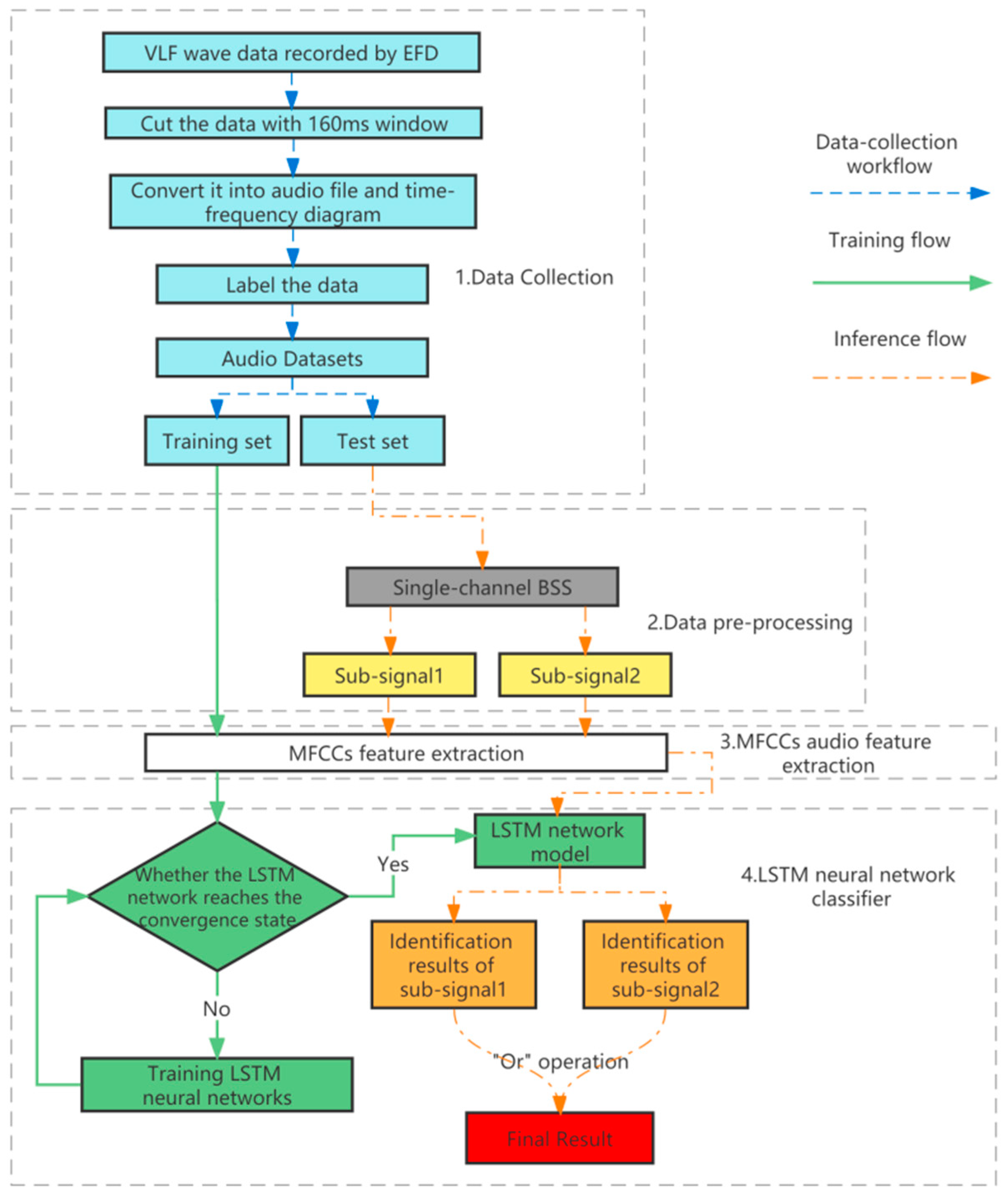
2. The Proposed Method

An LW event in EFD data (LW-EFD) is usually contaminated by other signal sources (e.g., signals from very low frequency (VLF) transmitters). Due to the short duration of LWs, their audio features were easily destroyed by these undesired signals, which decreases LW audio-recognition performance. To overcome the problem, we propose applying signal-separation techniques to reduce the interference from non-LW signals. The observation data in this paper come from a single-channel source (namely, the Z component of the EFD waveforms); meanwhile the number of mixed signals in the observed data and the mixing process were unknown. Therefore, this study adopted a single-channel blind source separation (SCBSS) algorithm to improve the LW audio-recognition algorithm, to reduce the influence of other electromagnetic disturbances, and to improve the performance of recognition of LWs from the EFD. The overall framework of the novel algorithm is shown in Figure 2; compared with the original method [17], the improvements were made mainly in the inference stage, which included four steps: data preprocessing, MFCC audio-feature extraction, LSTM neural network classification, and decision fusion. This section will mainly introduce these improvements.

2.1. Data Preprocessing

Each audio segment was considered as a single-channel observation signal. The single-channel blind source separation can obtain the source signal only according to the observed signal, which provides an effective solution for satellite signal analysis. With respect to the solution, there were three main families. The first kind is the model-based method, such as in Yilmaz et al. [18], which defined a weighted two-dimensional (2-D) histogram of time–frequency representations to separate mixed speech. Li-Na et al. [19] used the cepstrum peaks of speech signals to estimate the pitch period, separating voiced speech from mono speech. Mowlaee et al. [20] proposed a sinusoidal model-based algorithm, mainly consisting of a double-talk/single-talk detector and a minimum mean square error estimator to identify speaker and separate speech. Hershey et al. [21] adopted temporal dynamics model to separate speech. King et al. [22] separated the overlapping speech in the single-channel source by incorporating phase estimation via complex matrix factorization. Gao et al. [23] proposed an adaptive sparsity non-negative matrix factorization method for source separation and decomposed the mixture into a series of intrinsic mode functions without pretraining knowledge [24]. The second kind is the tuned signal feature-based method, such as in Warner et al. [25], which proposed an architecture for the blind separation of multiple, pulse-shaped multiphase phase-shift keying (MPSK) signals by means of a conventional independent component analysis (ICA) algorithm. Liao et al. [26] evaluated the multiphase phase-shift keying (MPSK) signal and the quadrature amplitude modulated (QAM) signal using the blind separation performance bound. Guo-Sheng et al. [27] estimated the amplitude for minimum shift keying (MSK) mixing signals in a single channel, improving the estimating accuracy by using the envelop values of leakage spectrum located at high-intensity spectral lines. Liang et al. [28] introduced the status of blind source separation (BBS) and studied some blind separation methods including transform domain filtering, multi-parameter joint estimation and so on. The third kind is the virtual multi-channel method, such as in Davies et al. [29] which identified when features of single-channel data can be used to extract independent components from a stationary scalar time series and stated that it was impossible to separate overlapping spectra sources by the standard ICA and the linear separation system. Hong et al. [30] separated periodic mechanical source signals from mixed signals in single-channel by combining the methods of wavelet decomposition and Fourier transform. Hong-Guang et al. [31] separated blind signals in single-channel by combining singular spectrum analysis (SSA) and blind source separation (BSS) techniques and proposed a segmentation method for nonstationary time series. Mijovi et al. [32] combined empirical-mode decomposition with ICA to separate and analyze biomedical signals with high noise-to-signal ratios. The model-based method was mainly suitable for the separation of mixed signals of speech and music signals, which required prior knowledge of the mixed signals. The tuned signal feature-based method was suitable for modulated speech signals, which required modulation prior to the signals; the virtual multi-channel-based method required less a priori information for single channel mixed signals and was suitable for the situation where there was no a priori knowledge. Since the CSES satellite electric field data in this study lacked the support of a priori knowledge, a SCBSS method based on virtual channels [33] was used to improve the old LW audio recognition model. The whole process, as shown in Figure 3, consisted of two parts: constructing a virtual multi-channel and blind source separation based on independent component analysis (ICA), which will be described in detail next.

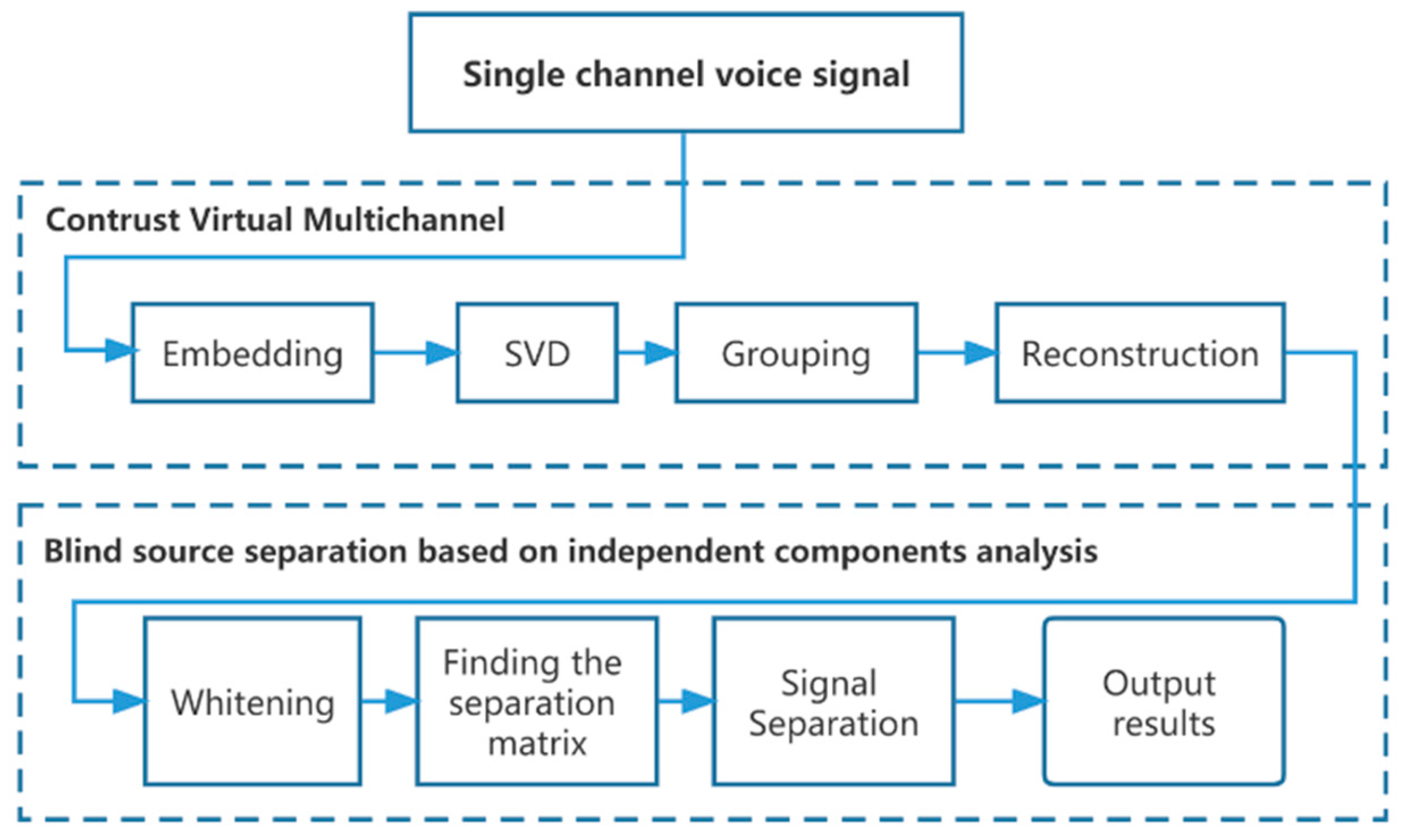
2.1.1. Construction of Virtual Multi-Channel

This subsection consists of four main implementation steps: embedding, singular value decomposition, grouping, and reconstruction.

A.

Embedding

The original waveform data have a sliding window of 160 ms, which contains 8192 evenly distributed points, denoted as ns sampling points. Therefore, for each audio signal, $x=\left[x_1,x_2,\dots ,x_{ns}\right]$, we chose an appropriate window length, L, and transformed the one-dimensional sequence into a trajectory matrix, X, as shown in Equation (1):

$$\mathit{X}=\left[\begin{array}{c}{x}_1\\ x_2\\ ⋮\\ x_M\end{array}\begin{array}{c}{x}_2\\ x_3\\ ⋮\\ x_{M+1}\end{array}\begin{array}{c}\dots \\ \cdots \\ ⋮\\ \cdots \end{array}\begin{array}{c}{x}_L\\ x_{L+1}\\ ⋮\\ x_{ns}\end{array}\right]=\left[{\mathit{x}}_1,{\mathit{x}}_2,\dots ,{\mathit{x}}_{\mathit{L}}\right]$$

(1)

where, $L=ns-M+1$. We set $M=128$ (details will be presented in the Discussion Section 4.1), $x_j={\left[x_j,x_{j+1},\dots ,x_{j+M-1}\right]}^T,\left(1\leqq j\leqq L\right)$. The trace matrix had the same elements on the opposite diagonal, and was called the Hankel matrix.

B.

SVD (singular value decomposition)

The singular value decomposition (SVD) of the trajectory matrix $X$ is computed as shown in Equation (2):

$$X=U\mathsf{\Sigma }{V}^T$$

(2)

where $U$ and $V$ were both unitary matrices satisfying $U{U}^T=I \mathrm{a}\mathrm{n}\mathrm{d} V{V}^T=I$, $U\in {\mathbb{R}}^{M\times M}$ was called the left singular matrix, $V\in {\mathbb{R}}^{L\times L}$ was called the right singular matrix, $\mathsf{\Sigma }\in {\mathbb{R}}^{M\times L}$ was a diagonal matrix with values only on the main diagonal, called singular values, and the remaining elements were all zeros. $\mathsf{\Sigma }$ had the following general form.

$$\mathsf{\Sigma }={\left[\begin{array}{c}{\sigma }_1\\ 0\\ 0\\ 0\end{array}\begin{array}{c}0\\ {\sigma }_2\\ 0\\ 0\end{array}\begin{array}{c}0\\ 0\\ \ddots \\ 0\end{array}\begin{array}{c}0\\ 0\\ 0\\ \ddots \end{array}\begin{array}{c}0\\ 0\\ 0\\ 0\end{array}\right]}_{M\times L}$$

(3)

If $U=\left[u_1,u_2,\dots ,u_M\right]$ and $V=\left[v_1,v_2,\dots ,v_L\right]$, Equation (2) was rewritten as Equation (4).

$$X=U\Sigma V^T={\sum }_{j=1}^M{\sigma }_j{u}_j{{(v}_j)}^T=X_1+X_2+\dots +X_M$$

(4)

where $X_j$ was the singular matrix corresponding to the singular value ${\sigma }_i$, called the singular sub-matrix of the matrix $X$.

C.

Grouping

Grouping aimed to divide the matrix $X$ into a set of linearly independent sub-matrices. According to the theorem that singular sub-matrix $X_i$ is independent of $X_j$ only if their singular values ${\sigma }_i\ne {\sigma }_j$, we divided the singular values $\left({\sigma }_1,{\sigma }_2,\cdots ,{\sigma }_L\right)$ into $\mathrm{d}$ groups, $l_1,l_2,\cdots ,l_d,$ and the trajectory matrix can be expressed as Equation (5):

$$X=X_{l_1}+X_{l_2}\cdots +X_{l_d}$$

(5)

where $X_{l_n}=\sum _{{\sigma }_j\in l_n}{\sigma }_j{u}_j{{(v}_j)}^T$. In the study, we divided $\left({\sigma }_1,{\sigma }_2,\cdots ,{\sigma }_L\right)$ into two groups: $l_1=\{{\sigma }_1,{\sigma }_2,\cdots ,{\sigma }_p\}$and $l_2=\left\{{\sigma }_{p+1},{\sigma }_{p+2},\cdots ,{\sigma }_L\right\} (\mathrm{w}\mathrm{h}\mathrm{e}\mathrm{r}\mathrm{e} {\sigma }_j\ne 0)$. Then, $X$ can be expressed as in Equation (6).

$$X=X_{l_1}+X_{l_2}$$

(6)

where $X_{l_1}=\sum _{j=1}^p{\sigma }_j{u}_j{{(v}_j)}^T$, $X_{l_2}=\sum _{j=p+1}^M{\sigma }_j{u}_j{{(v}_j)}^T$, $p$ was the parameter to be set, and $p=8$ was used in this paper; a detailed discussion is in Section 4.2.

D.

Signal reconstruction.

The matrices ${\mathit{X}}_{l_1}$ and ${\mathit{X}}_{l_2}$ were averaged inverse-diagonally according to Equation (7).

$$x_{l_{d,}k}=\left\{\begin{array}{c}\frac{1}{k}{\displaystyle \sum _{m=1}^k}{X}_{l_{d}m,k-m+1},1\le k<L^{\ast }=min\left\{M,L\right\}\\ \frac{1}{L^{\ast }}{\displaystyle \sum _{m=1}^{L^{\ast }}}{X}_{l_{d}m,k-m+1},L^{\ast }\le k\le K^{\ast }=max\left\{M,L\right\}\\ \frac{1}{ns-k+1}{\displaystyle \sum _{k-K^{\ast }+1}^{N-K^{\ast }+1}}{X}_{l_{d}m,k-m+1},{ K}^{\ast }<k\le ns\end{array}\right.\begin{array}{cc}& \\ & \\ & \end{array}$$

(7)

where $X_{l_d,p,q}$ denotes the element of the sub-matrix $X_{l_d}$ at position $\left(p,q\right)$. Finally, two sequences were obtained.

$${\mathcal{X}}_{l_1}={\left[{\mathcal{X}}_{l_{1}1},{\mathcal{X}}_{l_{1}2},\cdots {,\mathcal{X}}_{l_{1}ns}\right]}^T,{\mathcal{X}}_{l_2}={\left[{\mathcal{X}}_{l_{2}1},{\mathcal{X}}_{l_{2}2},\cdots {,\mathcal{X}}_{l_{2}ns}\right]}^T$$

(8)

2.1.2. Blind Source Separation Based on Independent Component Analysis (ICA)

Independent component analysis (ICA) was performed on the signal $\mathit{X}={\left({\mathit{x}}_{{\mathit{l}}_1},{\mathit{x}}_{{\mathit{l}}_2}\right)}^T\in {\mathbb{R}}^{2\times 8192}$.

A.

Whitening process

We whitened the signal $X$ to obtain mutually uncorrelated rows as shown in Equation (9).

$$\tilde{X}=E{D}^{\frac{1}{2}}{E}^{T}X$$

(9)

where $ED{E}^T$ was the eigenvalue decomposition of the covariance of $X$, i.e., $X{X}^T=ED{E}^T$.

B.

Finding the separation matrix$W^{\mathrm{*}}$

To find an optimal projection direction $W$, $\tilde{X}$ was projected into a direction which has the maximized non-Gaussianity. In this study, we used the negative entropy to measure the non-Gaussianity and made the mathematical model for finding the separation matrix $W$ in Equation (10).

$$\begin{gathered} W^{\ast }=arg max J_G\left(W\right)=\left[E\right\{G\left(W^T\tilde{X}\right)\}-E\{G\left({W^T\tilde{X}}_{gauss}\right\}{]}^2 \\ s.t.\left|\left|W^{T}W\right|\right|=1 \end{gathered}$$

(10)

where G denotes non-linear function and, in this study, was defined as $G\left(u\right)=-exp\left(-u^2/2\right)$, and ${W^T\tilde{X}}_{gauss}$ denotes a Gaussian random variable with the same covariance matrix as the variable $W^T\tilde{X}$. Finally, we use Lagrange multiplier method and Newton’s method in the paper [34] to figure out the model in Equation (10) to obtain the final $W$.

C.

Signal separation

The separation matrix $W^{\ast }$ was implemented on $\tilde{X}$ to produce the signal separation results $\widehat{S}$. The detail is expressed by Equation (11).

$$\widehat{S}={(\widehat{s_1},\widehat{s_2})}^T=W^{\ast T}\tilde{X}$$

(11)

where $\widehat{s_i}=\widehat{S}\left(i,:\right), 1\le i\le n$ (n = 2 in this paper).

Figure 4 illustrates an example of signal separation: the upper sub-figure displays the EFD waveform data, and the bottom sub-figure presents a time–frequency diagram. Figure 4a illustrates the source data. Figure 4b is the sub-signal $\widehat{s_2}$, which mainly contained the lightning whistler event. Figure 4c depicts the sub-signal $\widehat{s_1}$, which contained only the horizontal perturbation signal. Through the comparison among Figure 4a–c, it is evident that the LW in Figure 4b is much easier to recognize than in Figure 4a.

2.2. Audio Feature Extraction Stage

For the two sub-signals obtained from Section 3.1, their MFCC features are extracted by the method described in [17] and are illustrated in Figure 5. The MFCC map of the observed data in Figure 5a had a large region full of the strong energy. The MFCC map of the first sub-signals, denoted by MF$\widehat{s_1}$, is shown in Figure 5b. Figure 5c illustrates the MFCC map of the second sub-signals, denoted by MF$\widehat{s_2}$. Compared to Figure 5a, MF$\widehat{s_1}$ and MF$\widehat{s_2}$ demonstrate less red area, which indicates that some disturbance signals were reduced from the source data. It is worth noting that the second sub-signal MF$\widehat{s_2}$ in Figure 5c has only a very small area full of red, which means that the sub-signal MF$\widehat{s_2}$ is more clean than Figure 5a,b.

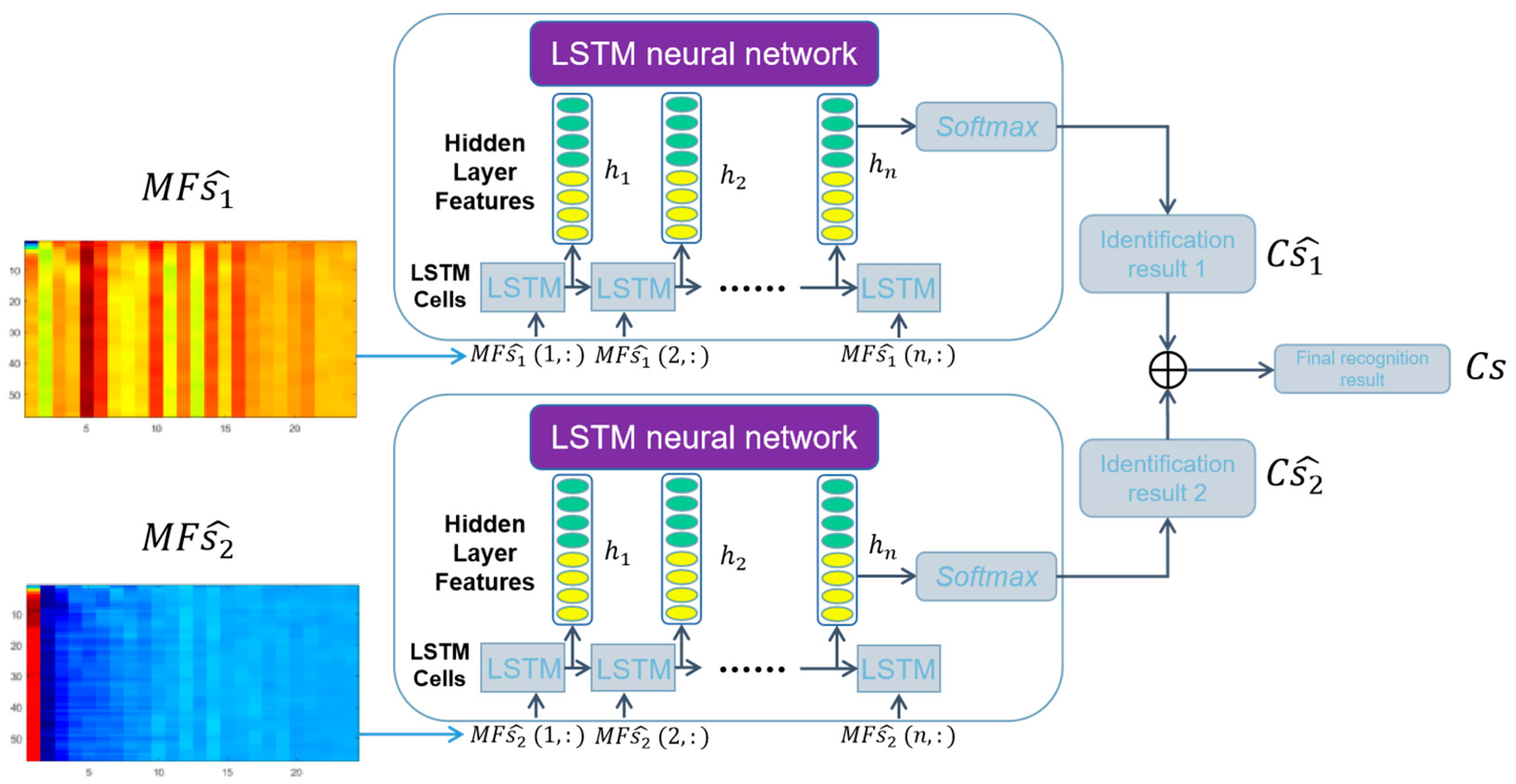
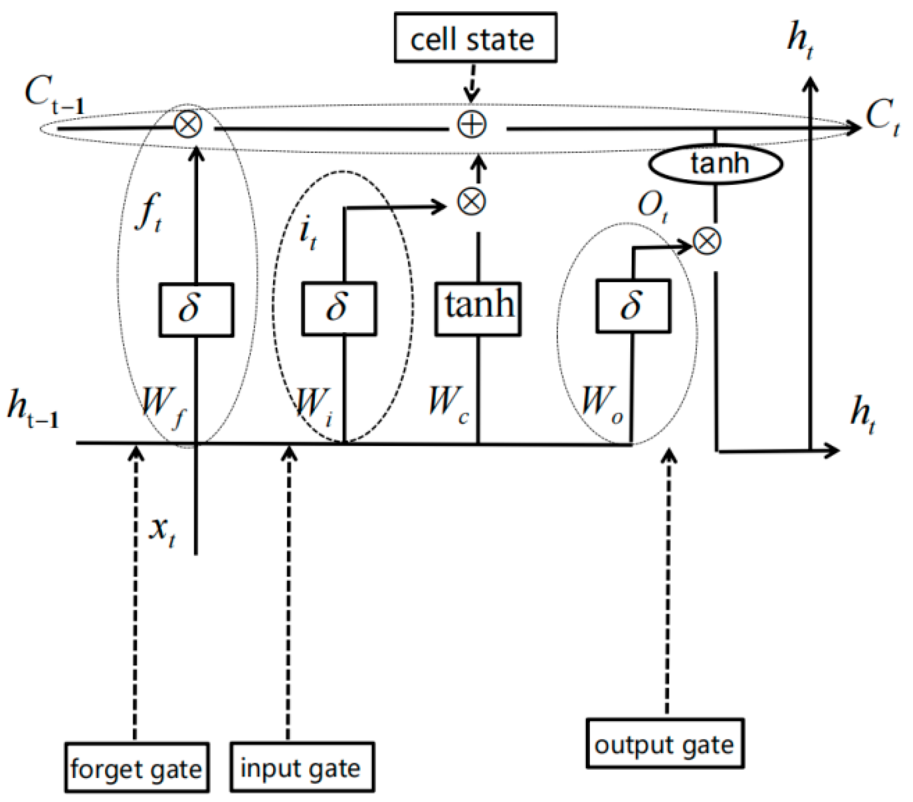
2.3. LSTM Neural Network Classification and Decision Fusion

The original data of the EFD are time series signals, and their MFCC features have obvious sequence correlation. LSTM is a type of neural network specifically fit for processing sequence-related data. In this subsection, classification and decision fusion will be conducted by a LSTM neural network as shown in Figure 6. MF$\widehat{s_1}$ and MF$\widehat{s_1}$ were input into the trained LSTM network to output the results $C_{\widehat{s_1}}\in \left\{0,1\right\}$ and $C_{\widehat{s_2}}\in \left\{0,1\right\}$, respectively (‘0′ means no LW, ‘1′ means LW). Finally, $C_{\widehat{s_1}}$ and $C_{\widehat{s_2}}$ were processed with the “or” operation as shown in Equation (12) to yield the final recognition result.

$$C_S=C_{\widehat{s_1}}⨁C_{\widehat{s_2}}$$

(12)

where $C_S\in \left\{0,1\right\}$ is the final recognition result and $\mathrm{“}⨁\mathrm{”}$ is the “or” operator.

The key element of the network is the LSTM cell unit, the structure of which is shown in Figure 7. It enables the network to “remember” long-term historical information, thereby capturing the dependency relationship between the current information and the historical information. The LSTM cell unit is mainly composed of four parts: cell state, forget gate f, input gate i, and output gate o.

The forget gate is used to determine which historical information needs to be discarded. The LSTM network learns to determine which content needs to be remembered. The forget gate is defined as follows:

$$f_t=\delta \left(W_t·\left[h_{t-1},x_t\right]+b_f\right)$$

(13)

where $x_t$ is the input of the network at time t, and it is the t-th MFCC value in the sequence. $\delta$ is the value of the sigmoid function. $W_t$ is the weight matrix at time t. $h_{t-1}$ represents the output feature of the LSTM network after inputting MFCC sequence data ${(x}_1,x_2,\dots ,x_{t-1})$. $b_f$ is the bias at time t. $f_t$ ranges from 0 to 1 and it represents the degree of forgetting at time t. A value of 0 represents complete forgetting, and 1 represents complete memory. The forget gate can filter out features unrelated to lightning whistle waves.

The input gate processes the current location data in the MFCC sequence. The sigmoid activation function at the left side of the middle part of Figure 7 is used to determine which features of the input date will be remembered. The input gate is defined as follows:

$$i_t=\delta \left(W_i·\left[h_{t-1},x_t\right]+b_i\right)$$

(14)

The cell state is a hidden state, which is an information container, storing relation information of the sequence data with historical memory. Its definition is as follows:

$$C_t=f_t\times C_{t-1}+i_t\times R_t$$

(15)

where $R_t$ (the candidate cell state) is the tanh of the part at the right of the input gate in Figure 7 and $R_t=\tanh \left(W_c·\left[h_{t-1},x_t\right]+b_c\right)$. It combines the last output and current input to calculate the current candidate cell state. Some information in the last cell state $C_{t-1}$ could be forgotten by combining the last cell state $C_{t-1}$ and forget gate $f_t$ through $f_t\times C_{t-1}$. Some information in the current candidate cell state $R_t$ could be remembered by combining the current candidate cell state $R_t$ and input gate $i_t$ through $i_t\times R_t$.

The output gate controls the output of the current hidden state, and the calculation is as follows:

$$o_t=\delta \left(W_o·\left[h_{t-1},x_t\right]+b_i\right)$$

(16)

where $o_t$ is the output gate. At first, the last output $h_{t-1}$ and the current input $x_t$ are sent to the sigmoid function. Then the current key information $h_t$ could be calculated as follows:

$$h_t=o_t\times \tanh \left(C_t\right)$$

(17)

$h_t$ is computed by combining the output gate $o_t$ and the current cell state $C_t$, containing correlation information among the sequence data, greatly improving the classification effect.

3. Experiments and Analysis

3.1. Datasets and Evaluation Metrics

The data set in this study was from the detailed survey of the EFD payload’s very low frequency (VLF) band during August 2019 from the CSES data [35]. Firstly, a sample wave was generated with a 160 ms window that included 8192 evenly distributed points, then it was converted into an audio file (i.e., wav) as a piece of sample. Secondly, a short-time Fourier transform analysis was implemented on an audio file to obtain its dynamic power spectra with a frequency resolution of 19.5 Hz and a time resolution of 0.5 ms. Thirdly, the MFCC speech feature matrix [22] was extracted from the audio data; for more concrete details, please refer to paper [10]. In short, we obtained a 16 × 39 matrix for each audio sample, where 16 and 39 denoted the number of frames and the number of MFCC features, respectively. Finally, the audio segments were manually labeled according to whether an L-shaped dispersion feature existed in the spectrogram. The data comprised 10,436 segments collected in August 2019, of which 5000 segments contained only LW, 4336 segments had no LW and no interference, 500 segments had LW and contained strong interference, and the remaining 500 segments contained only interference without LW.

Evaluation Metric: We used the following metrics to evaluate the performance of all methods [17]: accuracy, recall, F1-score, false alarm rate (FA), and missed alarm rate (MA), which were defined in the following Equations (18)–(22). The AUC (area under the curve) value is the area covered by the ROC (receiver operating characteristic) curve, and the larger the AUC value, the better the classification effect of the classifier. $\mathrm{A}\mathrm{U}\mathrm{C}\in [0,1]$.

$$Accuracy=\frac{TP+TN}{TP+FP+TN+FN}\in [0, 1]$$

(18)

$$Recall=\frac{TP}{TP+FN}\in [0, 1]$$

(19)

$$F1-score=\frac{1}{\left(TP+FP\right)/TP+\left(TP+FN\right)/TP}\in [0, 1]$$

(20)

$$FA=\frac{FP}{FP+TN}\in [0, 1]$$

(21)

$$MA=\frac{FP}{FP+TN}\in [0, 1]$$

(22)

where TP denotes the number of true positive cases, TN is the number of true negative cases, FN is the number of false negative cases, and FP represented the number of false positive cases. The higher the accuracy, recall, F1-score and ROC-AUC, the better, while the opposite is true for FA and MA.

Firstly, we randomly selected 10% of the LW-EFD data set as a validation for fine-tuning the hyper-parameters to obtain the final value as shown in

Table 2. Parameters.

	Parameter Name	Learning Rate	Batch-Size	Epoch	Optimizer	BSS_p	BSS_M
Extraction Method
MFCCs–LSTM		10 × 10−3	64	20	Adam	-	-
BSS–MFCCs–LSTM		10 × 10−3	64	20	Adam	8	128

Note: Where Learning rate indicates the learning rate of the neural network model, Batch indicates the number of training samples per batch, Epoch indicates the number of iterations during training, Optimizer indicates the optimizer used for the network model, Original indicates the original waveform as the feature, MFCCs_LSTM indicates the MFCCs were extracted from the original waveform as features, BSS_MFCCs_LSTM indicates that two sub-segments were obtained by BSS of the original waveform, and then MFCCs features were extracted from the sub-signal separately, P denotes the number of the first set of singular values, and M denotes the number of rows of the trajectory matrix.

. The maximum learning rate equaled 0.001, batch-size was 64, epoch was 20, and optimizer was Adam. Moreover, BSS_p, denoting the parameter p in Equation (6), was set to 8, BSS_M, representing the parameter M in Equation (1), was set to 128. Then, we randomly divided the LW-EFD dataset into the training set (30% of LW-EFD) and testing set (70% of LW-EFD). To evaluate the effectiveness of the proposed approach, BSS–MFCCs–LSTM, we used the previous method, MFCCs–LSTM [17], as a baseline and carried out 1000 rounds of experiments on the LW-EFD set.

3.2. Experimental Results

In this section, we will introduce the visualized and quantitative results to verify the effectiveness of our algorithm.

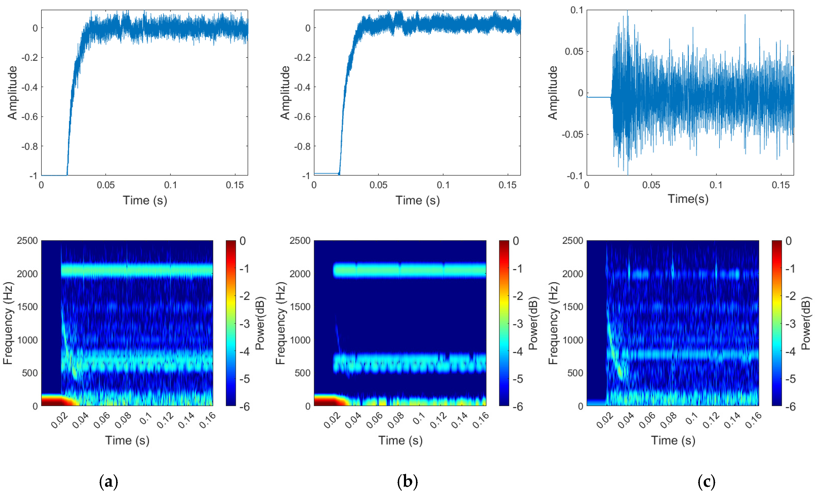
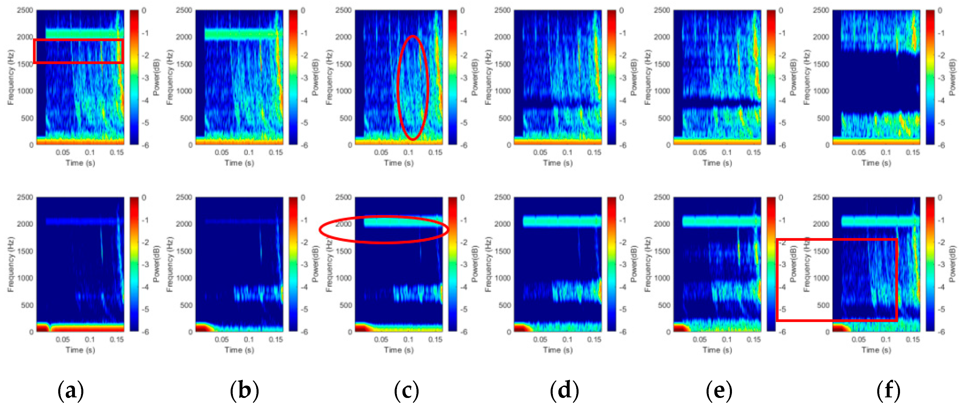
3.2.1. The Visualized Results

The visualized results are shown in Figure 8. The upper panels are the waveforms, and the lower panels are the time–frequency diagrams. Figure 8a illustrates the source data and tells us that it is rather challenging to identify an LW event from the noisy data, which is contaminated by lots of electromagnetic disturbances. The proposed method was implemented with SCBSS to yield two sub-signals, as shown in Figure 8b,c. It can be seen that recognizing the LW event from the sub-signal as shown in Figure 8c is not that difficult.

3.2.2. Quantitative Results

The works by paper [11] and the method of MFCCs–LSTM [17], which did not rely on GPU devices, were chosen as the baselines. We carried out 1000 rounds of experiments to compute the mean evaluation metrics (summarized in

Table 3. Performance.

	Recognition	Accuracy	Recall	F1-Score	ROC-AUC	FA	MA	Cost Time (s)	Cost Memory (MB)
Algorithm Evaluation Metrics
Works by Dharma et al. [11]		0.581 ± 0.021	0.236 ± 0.021	0.181 ± 0.021	0.678 ± 0.022	0.301 ± 0.019	0.78 ± 0.021	2.18 ± 0.117	68.1 ± 0.225
MFCCs–LSTM		0.573 ± 0.031	0.149 ± 0.065	0.253 ± 0.095	0.778 ± 0.049	0.002 ± 0.003	0.850 ± 0.065	2.240 ± 0.070	83.026 ± 0.560
BSS–MFCCs–LSTM		0.745 ± 0.050	0.771 ± 0.050	0.753 ± 0.028	0.821 ± 0.021	0.228 ± 0.143	0.279 ± 0.050	2.655 ± 0.050	128.210 ± 0.525

). In order to overcome the dependence on GPU equipment, a whistler recognition algorithm based on intelligent voice technology [17] has gained attention. However, compared with magnetic field data, the EFD data is very sensitive to noise, and the method of MFCCs–LSTM [17] cannot recognize lightning whistler events from EFD data interfered with by noise. In order to solve this problem, we have improved the method of MFCCs–LSTM [17] by adding a blind-source separation process to form the proposed method of BSS–MFCCs–LSTM, thereby increasing the time consumption and memory consumption slightly. As shown in Table 3, under the same conditions, the MFCCs–LSTM method consumes about 2.24 s, while the BSS–MFCCs–LSTM method consumes about 2.655s, an increase of about 0.41s. However, it can be seen from Table 3 that our BSS–MFCCs–LSTM had better performance on accuracy, recall, F1-Score, ROC_AUC, and MA metrics. It was noted that MFCCs–LSTM had an abnormally small effect on FA metrics. The reason for this was that the MFCCs–LSTM method cannot recognize LW samples with strong interference, which caused the FP in Equation (21) to be very low.

4. Discussion

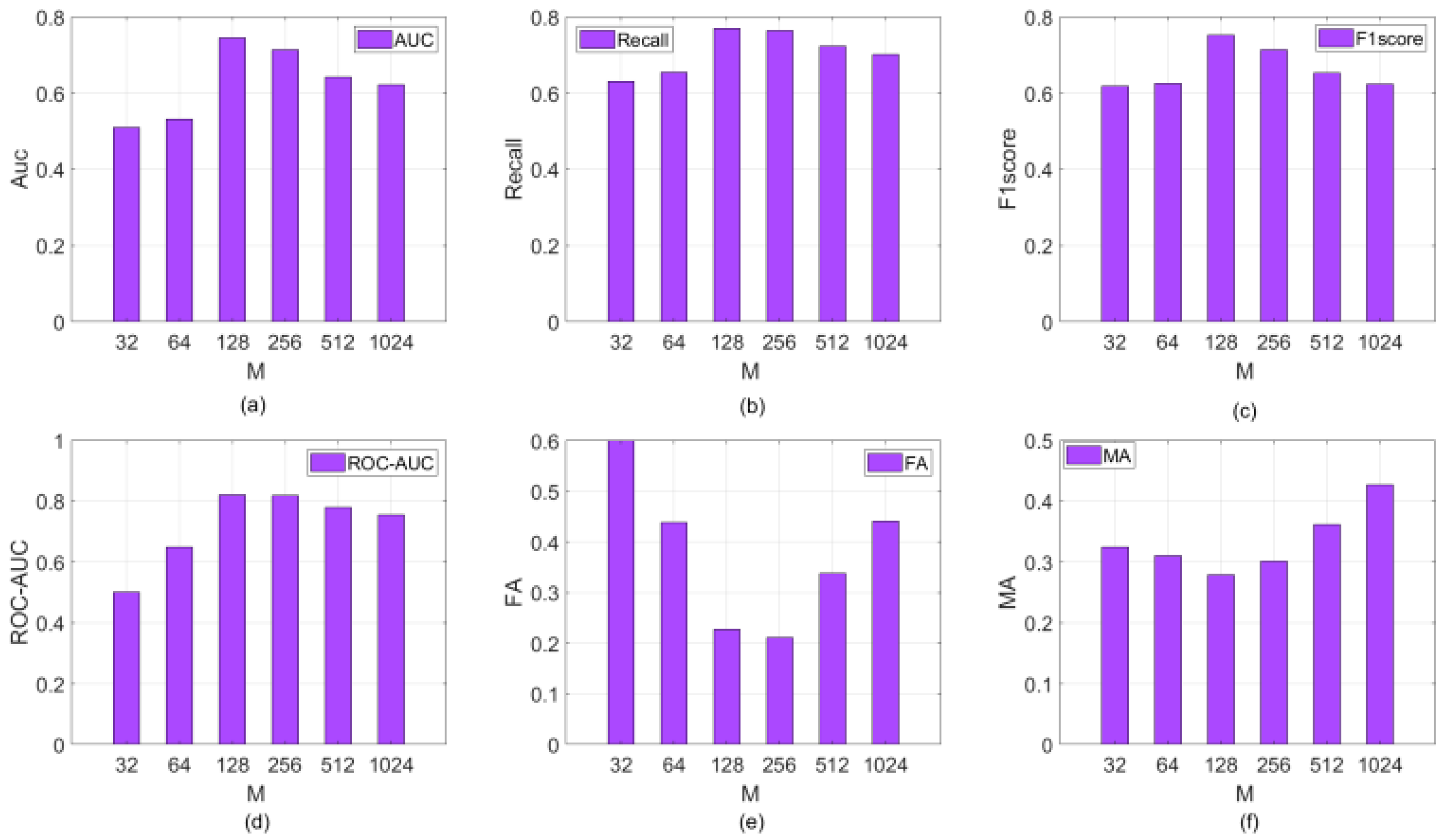
4.1. Impact of the Parameter M on the Performance of the Proposed Approach

An important parameter involved in BSS–MFCCs–LSTM was M; we explored the impact of different values of M on its performance in this subsection. With M varied from 32 to 1024, the quantitative results were plotted in Figure 9. It can be seen that when M was 128, the proposed method of BSS–MFCCs–LSTM (M = 128) could achieve a new state-of the-art in recognizing LW from the LW-EFD data set. The reason for this was that setting M = 128 could provide the best separated results by the SCBSS technique used in BSS–MFCCs–LSTM. To further explain it, we randomly selected a sample which contained an LW event and other electromagnetic signals, as shown in Figure 9. To see the details clearly, we illustrated the source signal in the frequency range from 0–2.5 kHz (Figure 10). For each value of the parameter p, the SCBSS was employed to handle the source signal to yield two sub-signals. In Figure 11, we depicted the time–frequency map of the 1st sub-signal and 2nd sub-signal in the left row and the right row, respectively. They revealed that when M < 128, the LW in the 1st sub-signal had been cut off at the band of 900 Hz, as marked with a red ellipse in Figure 11a, and when M > 128, the horizontal disturbance contaminated the first separated signal strongly, as marked with a rectangle in Figure 11e. Taking into comprehensive consideration the six metrics, the overall recognition performance was optimal at M = 128.

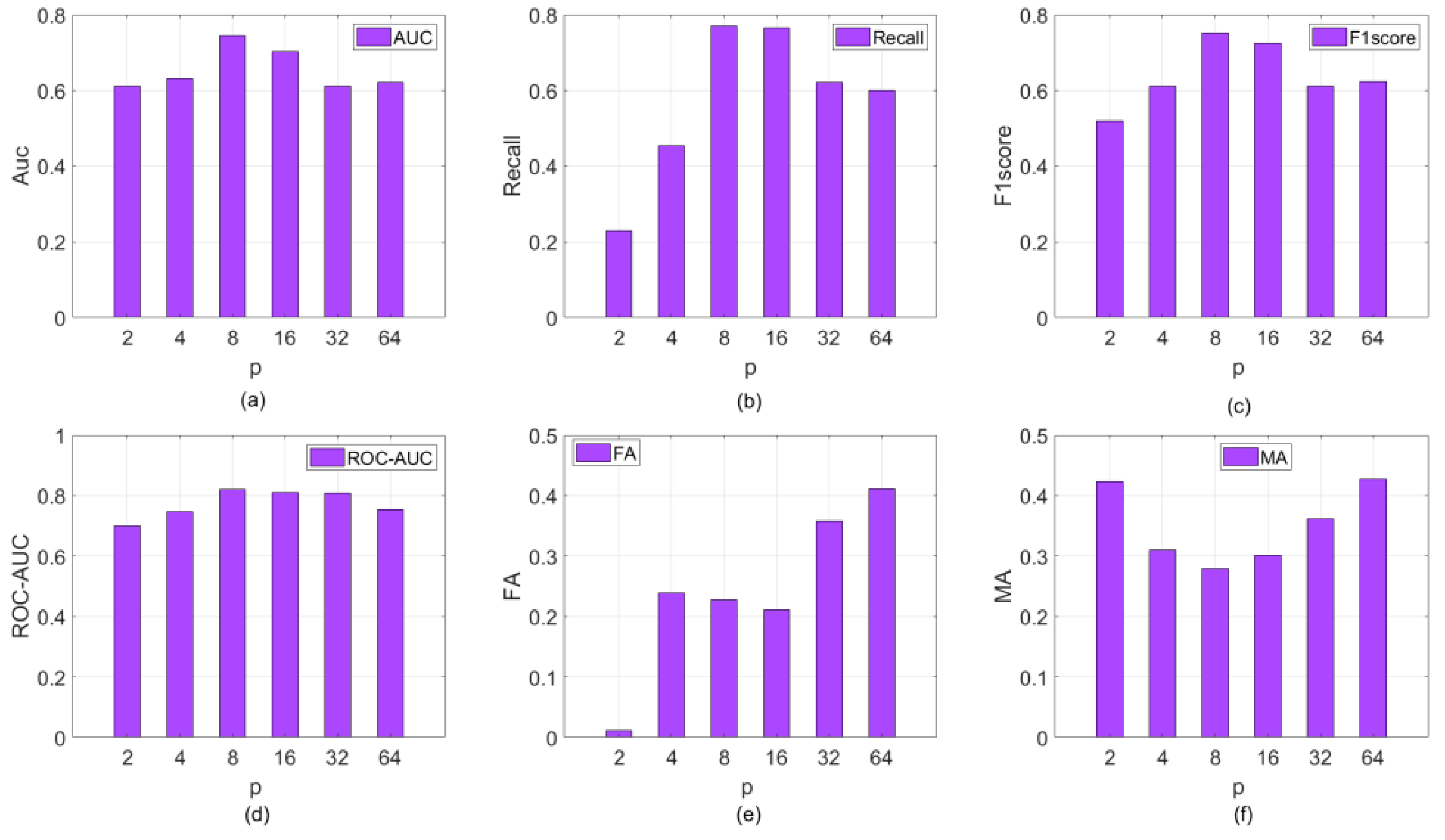
4.2. Impact of the Parameter p on the Performance of the Proposed Approach

In order to study the influence of different values of p on the performance of the proposed approach, we carried out experiments of varying values of p, with $\mathrm{p}\in \left\{\mathrm{2,4},\mathrm{8,16,32,64}\right\}$, to obtain the results illustrated in Figure 12. With the increasing of the p value, there was a trend that accuracy, recall, F1-score, and ROC-AUC first increased and then decreased, and another trend that MA first decreased and then increased. Special attention was paid to the trend of FA. When p = 4, the trend of FA was first decreased and then increased. However, at p = 2 the value of FA changes extremely little. To explain this further, a sample was separated by SCBSS with different values of p to yield sub-signals, as shown in Figure 13. Figure 13a is the time–frequency map of the two sub-signals separated by SCBSS (with p = 2) involving BSS–MFCCs–LSTM. It was easy to observe that the LW event in the first row of Figure 13a is contaminated strongly by the horizontal disturbance, as masked by the rectangle. This caused the LW event not to be identified. Further, it can significantly decrease the value of FP in Equation (22), thereby, causing the FA to fall to an extremely low value. Observed in Figure 13b–f, we found that at p = 8, the LW event and the horizontal disturbance were separated better than at other p values, masked by the ellipse. However, with increasing p, most of the LW event and the horizontal disturbance were mixed, such as in the rectangle area in Figure 13f. Taking Figure 12 and Figure 13 into comprehensive consideration, we could draw a conclusion that the optimal value of p was 8.

At present, values of M and p are selected manually through quantitative experiments and comparisons; establishing a method for determining the optimal parameters is an important issue to be studied in the future.

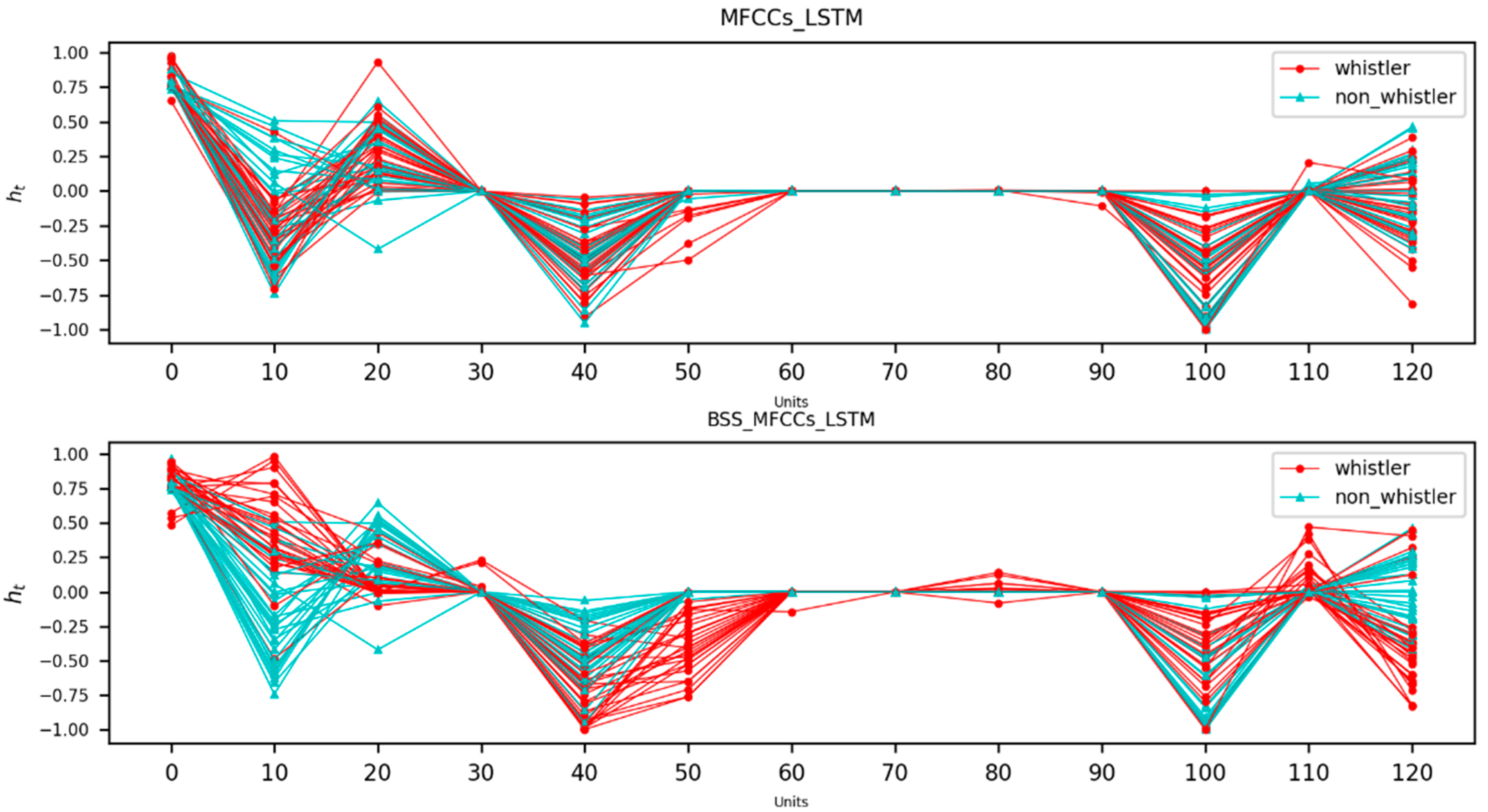
4.3. Visualization Results of Hidden-Layer Features of LSTM Neural Network

The hidden information features output by the hidden layer of the LSTM neural network model at the last moment are represented by $h_{\mathrm{t}}$. This abstract feature contains the historical and trend information of this time series, which will have a key impact on the final classification results. In this subsection, 60 samples (including 30 samples of lightning whistler with interference and 30 samples of non-lightning whistler with interference) were randomly selected from the test set of strong interference samples, and these samples were processed by two different algorithms (LSTM and BSS + LSTM) before being input to the LSTM neural network classifier model to determine their abstract information features in the hidden layer, and visualized as shown in Figure 14. Where the horizontal axis indicates the number of hidden units and the sequence length of $h_{\mathrm{t}}$, the vertical axis indicates the abstract feature values of the hidden layers. As can be seen from Figure 14, there are differences in the hidden-layer abstraction feature density between the MFCCs–LSTM algorithm and the BSS–MFCCs–LSTM algorithm for the lightning whistler with interference and the non-lightning whistler model with interference; the former has smaller inter-class variance and larger intra-class variance, while the latter has larger inter-class variance and smaller intra-class variance, which indicates that the features learned by the BSS–MFCCs–LSTM algorithm make it easier to achieve the classification of lightning whistlers.

5. Conclusions

The previous LW audio recognition algorithm (i.e., Yuan et al., [15]) had a poor performance when the LW events were contaminated severely by strong disturbances in the EFD data of the CSES. To overcome this limitation, this paper proposed a novel LW audio recognition algorithm with single-channel blind source separation (BSS–MFCCs–LSTM).

In the model inference stage, we employed SCBSS to handle the source data to yield two sub-signals. Then, the MFCCs for each sub-signal were extracted and input into the trained LSTM neural network to output two recognition results. Finally, they were computed by an “Or” operation to yield the final result. The experiments showed a clear improvement over previous methods in recognizing LW events from EFD data sets.

We examined the effects of two important parameters (i.e., M and p) on the performance on our approach. The results based on the EFD data of the CSES satellite demonstrate the effectiveness of the algorithm. The accuracy, recall and F1-score of this algorithm increased by 17%, 62.2%, and 50%, respectively, compared with classical methods. Moreover, the time-cost only increases by 0.41 s.

However, our algorithm was weak in the recognition of non-LW events with strong interference, which resulted in a worse FA. In our future work, the attention mechanism will be introduced to improve the algorithm.

References

1. Carpenter, D.L.; Anderson, R.R. An ISEE/Whistler model of equatorial electron density in the magnetosphere. J. Geophys. Res. Space Phys. 1992, 97, 1097–1108. [Google Scholar] [CrossRef]
2. Bayupati, I.P.A.; Kasahara, Y.; Goto, Y. Study of Dispersion of Lightning Whistlers Observed by Akebono Satellite in the Earth’s Plasmasphere. IEICE Trans. Commun. 2012, E95-B, 3472–3479. [Google Scholar] [CrossRef]
3. Oike, Y.; Kasahara, Y.; Goto, Y. Spatial distribution and temporal variations of occurrence frequency of lightning whistlers observed by VLF/WBA onboard Akebono. Radio Sci. 2015, 49, 753–764. [Google Scholar] [CrossRef]
4. Chen, Y.; Ni, B.; Gu, X.; Zhao, Z.; Yang, G.; Zhou, C.; Zhang, Y. First observations of low latitude whistlers using WHU ELF/VLF receiver system. Sci. China (Technol. Sci.) 2017, 60, 166–174. [Google Scholar] [CrossRef]
5. Kishore, A.; Deo, A.; Kumar, S. Upper atmospheric remote sensing using ELF–VLF lightning generated tweek and whistler sferics. South Pac. J. Nat. Appl. Sci. 2016, 34, 12. [Google Scholar] [CrossRef]
6. Záhlava, J.; Němec, F.; Pincon, J.L.; Santolík, O.; Kolmaová, I.; Parrot, M. Whistler Influence on the Overall Very Low Frequency Wave Intensity in the Upper Ionosphere. J. Geophys. Res. Space Phys. 2018, 123, 5648–5660. [Google Scholar] [CrossRef]
7. Parrot, M.; Pinçon, J.-L.; Shklyar, D. Short-Fractional Hop Whistler Rate Observed by the Low-Altitude Satellite DEMETER at the End of the Solar Cycle 23. J. Geophys. Res. Space Phys. 2019, 124, 3522–3531. [Google Scholar] [CrossRef]
8. Horne, R.B.; Glauert, S.A.; Meredith, N.P.; Boscher, D.; Maget, V.; Heynderickx, D.; Pitchford, D. Space weather impacts on satellites and forecasting the Earth’s electron radiation belts with SPACECAST. Space Weather-Int. J. Res. Appl. 2013, 11, 169–186. [Google Scholar] [CrossRef]
9. Lichtenberger, J.; Ferencz, C.; Bodnár, L.; Hamar, D.; Steinbach, P. Automatic Whistler Detector and Analyzer system: Automatic Whistler Detector. J. Geophys. Res. Space Phys. 2008, 113. [Google Scholar] [CrossRef]
10. The Stanford VLF Group Automated Detection of Whistlers for the TARANIS Spacecraft Overview of the Project. 2009. Available online: https://vlfstanford.ku.edu.tr/research_topic_inlin/automated-detection-whistlers-taranis-spacecraft/ (accessed on 15 August 2023).
11. Dharma, K.S.; Bayupati, I.; Buana, P.W. Automatic Lightning Whistler Detection Using Connected Component Labeling Method. J. Theor. Appl. Inf. Technol. 2014, 66, 638–645. [Google Scholar] [CrossRef]
12. Fiser, J.; Chum, J.; Diendorfer, G.; Parrot, M.; Santolik, O. Whistler intensities above thunderstorms. Ann. Geophys. 2010, 28, 37–46. [Google Scholar] [CrossRef]
13. Zhou, R.X.; Gu, X.D.; Yang, K.X.; Li, G.S.; Ni, B.B.; Yi, J.; Chen, L.; Zhao, F.T.; Zhao, Z.Y.; Wang, Q.; et al. A detailed investigation of low latitude tweek atmospherics observed by the WHU ELF/VLF receiver: I. Automatic detection and analysis method. Earth Planet. Phys. 2020, 4, 120–130. [Google Scholar] [CrossRef]
14. Ali Ahmad, U.; Kasahara, Y.; Matsuda, S.; Ozaki, M.; Goto, Y. Automatic Detection of Lightning Whistlers Observed by the Plasma Wave Experiment Onboard the Arase Satellite Using the OpenCV Library. Remote Sens. 2019, 11, 1785. [Google Scholar] [CrossRef]
15. Konan, O.J.E.Y.; Mishra, A.K.; Lotz, S. Machine Learning Techniques to Detect and Characterise Whistler Radio Waves. arXiv 2020, arXiv:2002.01244. [Google Scholar] [CrossRef]
16. Yuan, J.; Wang, Q.; Yang, D.H. Automatic recognition algorithm of lightning whistlers observed by the Search Coil Magnetometer onboard the Zhangheng-1 Satellite. Chin. J. Geophys. 2021, 64, 3905–3924. [Google Scholar] [CrossRef]
17. Yuan, J.; Wang, Z.J.; Zeren, Z.M.; Wang, Z.G.; Feng, J.L.; Shen, X.H.; WU, P.; Wang, Q.; Yang, D.H.; Wang, T.L.; et al. Automatic recognition algorithm of the lightning whistler waves by using speech processing technology. Chin. J. Geophys. 2022, 65, 882–897. [Google Scholar]
18. Yilmaz, O.; Rickard, S. Blind Separation of Speech Mixtures via Time-Frequency Masking. IEEE Trans. Signal Process. 2004, 52, 1830–1847. [Google Scholar] [CrossRef]
19. Li-Na, Z.; Er-Hua, Z.; Jun-Liang, J. Monaural voiced speech separation based on computational auditory scene analysis. Comput. Eng. Sci. 2019, 41, 1266–1272. [Google Scholar] [CrossRef]
20. Mowlaee, P.; Saeidi, R.; Christensen, M.G.; Zheng-Hua, T.; Kinnunen, T.; Franti, P.; Jensen, S.H. A Joint Approach for Single-Channel Speaker Identification and Speech Separation. IEEE Trans. Audio Speech Lang. Process. 2012, 20, 2586–2601. [Google Scholar] [CrossRef]
21. Hershey, J.R.; Rennie, S.J.; Olsen, P.A.; Kristjansson, T.T. Super-human multi-talker speech recognition: A graphical modeling approach. Comput. Speech Lang. 2010, 24, 45–66. [Google Scholar] [CrossRef]
22. King, B.J.; Atlas, L. Single-Channel Source Separation Using Complex Matrix Factorization. IEEE Trans. Audio Speech Lang. Process. 2011, 19, 2591–2597. [Google Scholar] [CrossRef]
23. Gao, B.; Woo, W.L.; Dlay, S.S. Adaptive Sparsity Non-Negative Matrix Factorization for Single-Channel Source Separation. IEEE J. Sel. Top. Signal Process. 2011, 5, 988–1001. [Google Scholar] [CrossRef]
24. Gao, B.; Woo, W.L.; Dlay, S.S. Single-Channel Source Separation Using EMD-Subband Variable Regularized Sparse Features. IEEE Trans. Audio Speech Lang. Process. 2011, 19, 961–976. [Google Scholar] [CrossRef]
25. Warner, E.S.; Proudler, I.K. Single-channel blind signal separation of filtered MPSK signals. IEE Proc.-Radar Sonar Navig. 2003, 150, 396–402. [Google Scholar] [CrossRef]
26. Liao, C.; Wan, J.; Zhou, S. Single-channel blind separation performance bound of two co-frequency modulated signals. J. Tsinghua Univ. 2010, 50, 1646–1650. [Google Scholar] [CrossRef]
27. Rui, G.S.; Xu, B.; Zhang, S. Amplitude estimating algorithm for single channel mixing signals. J. Commun. 2011, 32, 82–87. [Google Scholar]
28. Liang, W.U.; Hua, J. Blind separation algorithm of single-channel mixed-signal. Inf. Electron. Eng. 2012, 10, 343–349. [Google Scholar] [CrossRef]
29. Davies, M.E.; James, C.J. Source separation using single channel ICA. Signal Process. 2007, 87, 1819–1832. [Google Scholar] [CrossRef]
30. Hong, H.; Liang, M. Separation of fault features from a single-channel mechanical signal mixture using wavelet decomposition. Mech. Syst. Signal Process. 2007, 21, 2025–2040. [Google Scholar] [CrossRef]
31. Ma, H.-G.; Jiang, Q.-B.; Liu, Z.-Q.; Liu, G.; Ma, Z.-Y. A novel blind source separation method for single-channel signal. Signal Process. 2010, 90, 3232–3241. [Google Scholar] [CrossRef]
32. Mijović, B.; De Vos, M.; Gligorijevic, I.; Taelman, J.; Van Huffel, S. Source Separation From Single-Channel Recordings by Combining Empirical-Mode Decomposition and Independent Component Analysis. IEEE Trans. Biomed. Eng. 2010, 57, 2188–2196. [Google Scholar] [CrossRef] [PubMed]
33. Maddirala, A.K.; Shaik, R.A. Separation of Sources From Single-Channel EEG Signals Using Independent Component Analysis. IEEE Trans. Instrum. Meas. 2018, 67, 382–393. [Google Scholar] [CrossRef]
34. Ji, L.; Zhuang, H.; Cheng, D.; Yi, C. Blind Source Separation of Single-Channel Background Sound Cockpit Voice Based on EEMD and FastICA. J. Technol. 2021, 21, 62–67,74. [Google Scholar] [CrossRef]
35. Diego, P.; Bertello, I.; Candidi, M.; Mura, A.; Coco, I.; Vannaroni, G.; Ubertini, P.; Badoni, D. Electric field computation analysis for the Electric Field Detector (EFD) on board the China Seismic-Electromagnetic Satellite (CSES). Adv. Space Res. 2017, 60, 2206–2216. [Google Scholar] [CrossRef]
Figure 1. Lightning-generated whistler recorded by the EFD (electric field detector) onboard the CSES.
Atmosphere 14 01633 g001
Figure 2. The framework of the proposed audio recognition for lightning whistlers recorded by the EFD onboard the CSES satellite.
Atmosphere 14 01633 g002
Figure 3. Single-channel blind source separation based on virtual multi-channel.
Atmosphere 14 01633 g003
Figure 4. Results: (a) source data; (b) the first sub-signal; (c) the second sub-signal.
Atmosphere 14 01633 g004
Figure 5. Audio features: (a) original data; (b) MFCC map of the first sub-signal; (c) MFCC map of the second sub-signal.
Atmosphere 14 01633 g005
Figure 6. LSTM neural network classification and decision fusion.
Atmosphere 14 01633 g006
Figure 7. The unit structure of the LSTM cell.
Atmosphere 14 01633 g007
Figure 8. Results by using SCBSS: (a) source data; (b) sub-signal 1; (c) sub-signal 2.
Atmosphere 14 01633 g008
Figure 9. Recognition results varied with different values of M: (a) 32; (b) 64; (c) 128; (d) 256; (e) 512; (f) 1024.
Atmosphere 14 01633 g009
Figure 10. An example of source data.
Atmosphere 14 01633 g010
Figure 11. Visualized results varied with different values of M: (a) 32; (b) 64; (c) 128; (d) 256; (e) 512; (f) 1024.
Atmosphere 14 01633 g011
Figure 12. Recognition results varied with different values of p: (a) AUC; (b) Recall; (c) F1score; (d) ROC-AUC; (e) FA; (f) MA.
Atmosphere 14 01633 g012
Figure 13. Visualized results varied with different values of p: (a) 2; (b) 4; (c) 8; (d) 16; (e) 32; (f) 64.
Atmosphere 14 01633 g013
Figure 14. Visualization results of hidden-layer features of LSTM neural networks under different algorithms (MFCCs–LSTM, BSS–MFCCs–LSTM).
Atmosphere 14 01633 g014