1. Introduction
Wildland fires are a naturally occurring phenomenon, the impacts of which can be exacerbated or ameliorated by human actions. Fire plays an essential role in many ecosystems, but when not adequately managed, it can have disastrous impacts on natural systems and human lives and assets. Indeed, many of the wildland fires that have occurred around the world over the last two decades constitute significant natural disasters, particularly in regions such as southeastern Australia and western North America [
1,
2,
3]. Anthropogenic climate change is also affecting fire occurrence and severity around the globe and is a likely driver of the increase in the frequency of very large and destructive wildland fires that have been observed [
4,
5,
6]. The Black Summer fires that occurred during 2019–2020 over southeastern Australia serve as a particularly telling example. These fires burnt over the course of several months and directly caused 33 deaths, including 26 civilians and seven firefighters [
7]. Extensive smoke from the fires resulted in almost 450 additional deaths due to smoke inhalation and affected around 80% of the population [
8,
9]. It is further estimated that in excess of one billion animals perished in the fires [
10].
Wildfire management, which encompasses risk assessment and decision-making, ecological considerations, strategic fuel management, and fire suppression (direct or indirect), has an important role to play in mitigating wildfire impact. It requires considerable resources, which need to be deployed in a cost-effective manner. Wildfire spread prediction is critical in supporting decision-making related to the deployment of resources, suppression tactics, the issuance of public evacuation orders, and other aspects of wildfire management and emergency response.
Mathematical models of wildfire spread have been developed to predict fire behavior since the 1940s [
11]. There are different types of fire behavior models, including empirical and semi-empirical models, such as artificial intelligent (AI) models, which are based on experiments and historical data, and physics-based models that are based on physical and mathematical relationships between inputs and the rate of fire spread [
12]. Because of their computational simplicity, empirical models are usually preferred [
13] in most operational systems, and for this reason, empirical models are used in this study for developing the rate of fire spread.
Two-dimensional empirical and semi-empirical fire propagation models were established based on an anisotropic Huygens principle [
14]. These models typically require weather inputs such as wind, temperature, relative humidity, and the moisture content of the fuel, as well as fuel and topographic conditions. Fire propagation is particularly sensitive to variations in wind speed and direction [
15]. The rate of fire propagation is approximately proportional to the square of wind speed (when >
) [
16]. This effect can be further increased under certain conditions, such as when fuel moisture content is low. As such, spatial and temporal variations in wind inputs can have significant impacts on the propagation of a fire [
17,
18]. Spatio-temporal variation in the wind field, along with variations in the other driving factors, can cause a considerable range of uncertainty in the prediction of fire spread, so much so that it is considered routine for actual fire spread to differ from the predicted fire spread by a factor of ±30% [
19]. Therefore, the inclusion of wind models that account for the intrinsic uncertainty of the wind field and understanding how they might influence the output of operational fire propagation models represent important aspects of effective fire risk management [
20,
21].
In order to better accommodate the influence of the spatial and temporal variability of weather-related factors in fire spread prediction, modelers have pursued various probabilistic approaches. In one approach, which is here referred to as the “deterministic ensemble” approach, weather inputs are repeatedly sampled from a particular probability distribution. Each of the sampled input datasets is then applied in a deterministic fire-spread model, providing an ensemble of possible fire-spread outcomes. In the most basic implementations of the deterministic ensemble approach, fire weather inputs are sampled from standard probability distributions, such as the uniform distribution (e.g., Fire
ds [
22]) or the normal distribution (e.g.,
spark [
23]), whereas in more sophisticated implementations, the forecast and historical data are combined to produce a more faithful statistical characterization of weather inputs at a particular location (e.g.,
wfdss [
24]). This deterministic ensemble approach was also applied in the context of one-dimensional rate-of-spread prediction by [
25], who sampled input conditions from a normal distribution but also noted the potential use of the Weibull distribution for sampling wind speed. Hilton et al. [
26] and Dabrowski et al. [
17] incorporated random components in a fire propagation model, which resulted in a probabilistic technique for predicting wildfire propagation.
Specifically, Hilton et al. [
26] added the spatial and temporal variation of environmental factors, such as combustion condition, wind speed, and wind direction, to the rate of fire spread prediction based on the level set method. The variation in the elements was investigated by picking random values for the inputs from a Gaussian distribution with a prescribed standard deviation. The resultant simulations compared favorably with observed grassland fires, thus highlighting the potential improvements that such an approach could have in fire propagation modeling. The analyses carried out by [
26] demonstrated that variation in the combustion condition slows the rate of fire growth and creates an irregular fire front, whereas wind variation produces more rounded flanks and alters the geometric shape of the fire perimeter for simulations initialized with a straight fire line. Although this study introduced some randomness to fire spread simulation, the simulations generated roughly symmetrical fire perimeters that did not show any indication of natural variability of wind over time, nor did it consider ensemble runs to assess the spatial variability of risk.
Although deterministic ensemble approaches, along with other probabilistic wildfire spread models, such as [
26], account for variability in a wind field and other driving factors, they do not really acknowledge the inherent stochasticity of the wind vector, nor do they acknowledge the process-based nature of wind variability [
27].
On the other hand, in other areas of study related to wind modeling, e.g., for wind energy applications and wind farms, the wind is explicitly treated as a stochastic variable [
28]. Indeed, there have been several studies that have treated wind as a stochastic process. Bivona et al. [
27] developed a class of stochastic models for an hourly averaged wind speed time series using the models of [
29]. The proposed stochastic models were then evaluated for wind speed time series recorded in two regions in Italy over four years, and it was found that the results captured the wind speed distributions in
of cases.
The Ornstein-Uhlenbeck (
ou) process, also known as the “First-Order Gauss-Markov (
fogm) process”, has been frequently utilized for wind modeling, especially in applications related to wind power generation. Arenas et al. [
30] considered the relationship between mean wind speed and turbulence intensity using the
ou process to capture wind speed variability, and wind magnitude and direction data at altitudes of up to 20 km were used by Turkoglu et al. [
31] to calibrate an
ou process model to better inform real-time guidance strategies in avionics applications. Their results showed that the wind simulations reasonably imitate the stochastic nature of the wind characteristics. Zarate et al. [
32] applied the continuous format of stochastic differential equations (Wiener process) to generate wind speed profiles with statistical properties, including mean, variance, and autocorrelation. These profiles were constructed based on historical wind speed data for a specific location and were designed to be suitable for power system dynamic studies.
Benth et al. [
33] investigated the correlation between electricity prices and wind power production in wind energy markets. Specifically, they modeled wind speed using the
ou process and calibrated the parameters based on wind observations, with the practical intention of helping inform business strategy and risk assessment for energy producers. Loukatou et al. [
28] also showed the advantage of a dynamic representation in continuous time for random wind speed variation through the application of the
ou process.
Stochastic process models have also seen some limited use in bushfire modeling applications. For example, Zazali et al. [
34] considered a basic deterministic bushfire model and incorporated stochasticity in the model by treating wind speed and direction as Wiener processes. They compared the resulting stochastic model with corresponding deterministic ensembles and demonstrated that the stochastic model generated a broader range of possible fire perimeters than the deterministic ensemble approach.
In the present study, we attempt to accommodate the environmental uncertainty that arises due to temporal variations in the wind vector in a wildfire spread model within the two-dimensional fire simulation platform
spark [
35], which models fire propagation using a level set-based approach [
26]. We model the wind vector using two different stochastic processes, namely the Wiener process and the
fogm process, using the wind observations of Quil et al. [
20] to calibrate the required parameters. The stochastic wind models are then incorporated within the workflow of
spark.
3. Data Analysis and Stochastic Wind Simulations
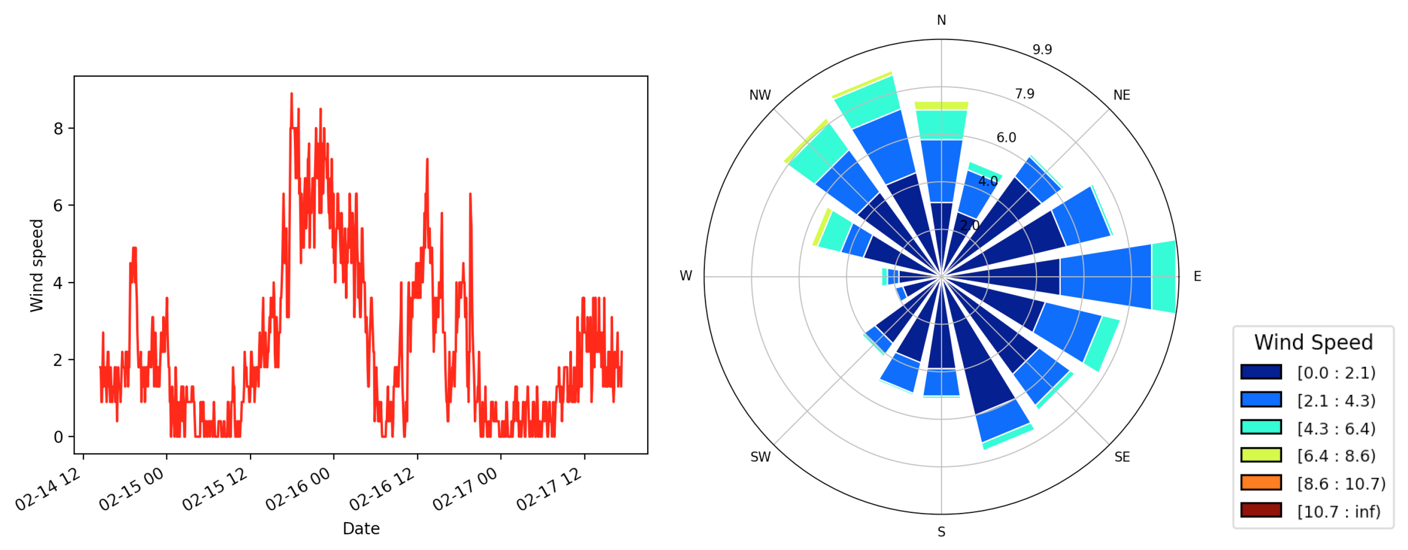
In this section, the primary goal is to harness historical wind data collected at a 5 min sampling rate to derive reliable estimates of the stochastic process noises to quantify the variability in the wind. This approach enables the capture of sub-hourly temporal wind variability, which can then be incorporated into a fire simulation model when the sub-hourly wind data are not available. The aim is to gain a deeper understanding of the inherent variability and uncertainty within wind patterns. This understanding is crucial, especially when simulating scenarios within a fire spread model, where accurately representing the dynamic nature of wind can significantly impact the reliability of predictions. This becomes particularly valuable for regions or times with sparse wind observations, allowing us to fill in the gaps and provide more reliable predictions.
3.1. Stochastic Process Calibration
In this section, the magnitude of each of the stochastic process noise parameters
, and
in Equations (
3) and (
4) are calibrated using anemometer data collected from a field site close to Canberra Airport [
36]. The collection period was divided into hourly blocks, as this reflects operational time frames, i.e., wind conditions are typically reported on an hourly basis. Hence, the calibration of the process noises of the random walk and
fogm processes are estimated over every hourly block, and a time step of 5 min is used as
in both stochastic processes. In order to calculate the magnitude of the stochastic noises, the point-to-point variance in consecutive wind data
is calculated within each hourly block. For the random walk process, based on Equation (
3), this value is then divided by the square root of the sampling rate of the data, which is 5 min. Additionally, for the
fogm process, the calculated variance, the sampling rate, and the correlation time are substituted into Equation (
5) to determine the process noise
and
for each of the wind components.
When considering each of the hourly intervals for each of the 11 anemometers, this yielded thousands of estimates of the process noises. These were averaged for each weather station and applied in simulations to model the wind vector components. The mean of the estimated values for the random walk process noise over all the stations was calculated as
for the
x and
y components
, and the calculated mean process noise for the
fogm process is
. The calibrated process noise components for all stations are listed in
Table 1 and
Table 2.
3.2. Wind Simulations
After the calibration of the process noise parameters, the stochastic wind models were implemented to predict the wind vector during a specific period. This prediction needs to be evaluated by comparing it with the observed wind data. For the evaluation of the two stochastic process models, the estimated mean process noise, calibrated using data collected over a two-month period from 11 weather stations and hourly blocks, was applied to simulate the wind components for each hourly block. While the same mean process noise was applied to all the hourly blocks, the initial wind observation for each hourly block was used as the initial value for each simulation. An alternative approach would be to generate a set of random initial points around the observed initial value, generate a set of simulations over the selected period, and eventually use the mean of all the simulations. However, due to the mean-reverting property of the fogm process, the mean of these simulations would not be significantly different from a simulation starting from the observed initial value. Moreover, the standard deviation of the observed data in the particular experiment carried out here is small enough that an average of such simulated data would be insignificantly different from a simulation using the actual observed value for both the fogm and random walk processes.
The correlation time in the fogm process was chosen to be 5 h. For the observed wind data of this study, we evaluated the discrepancy between the observed data and simulated data when using different correlation times for the fogm process and discovered that a correlation time of ∼5 h (for hourly blocks of wind data) gives the closest simulations to the observations. Sensitivity analyses were also carried out to examine the effect of using different correlation times, ranging from 5 min to 10 h. These analyses revealed that varying the correlation time across this range of values had minimal impact on the results.
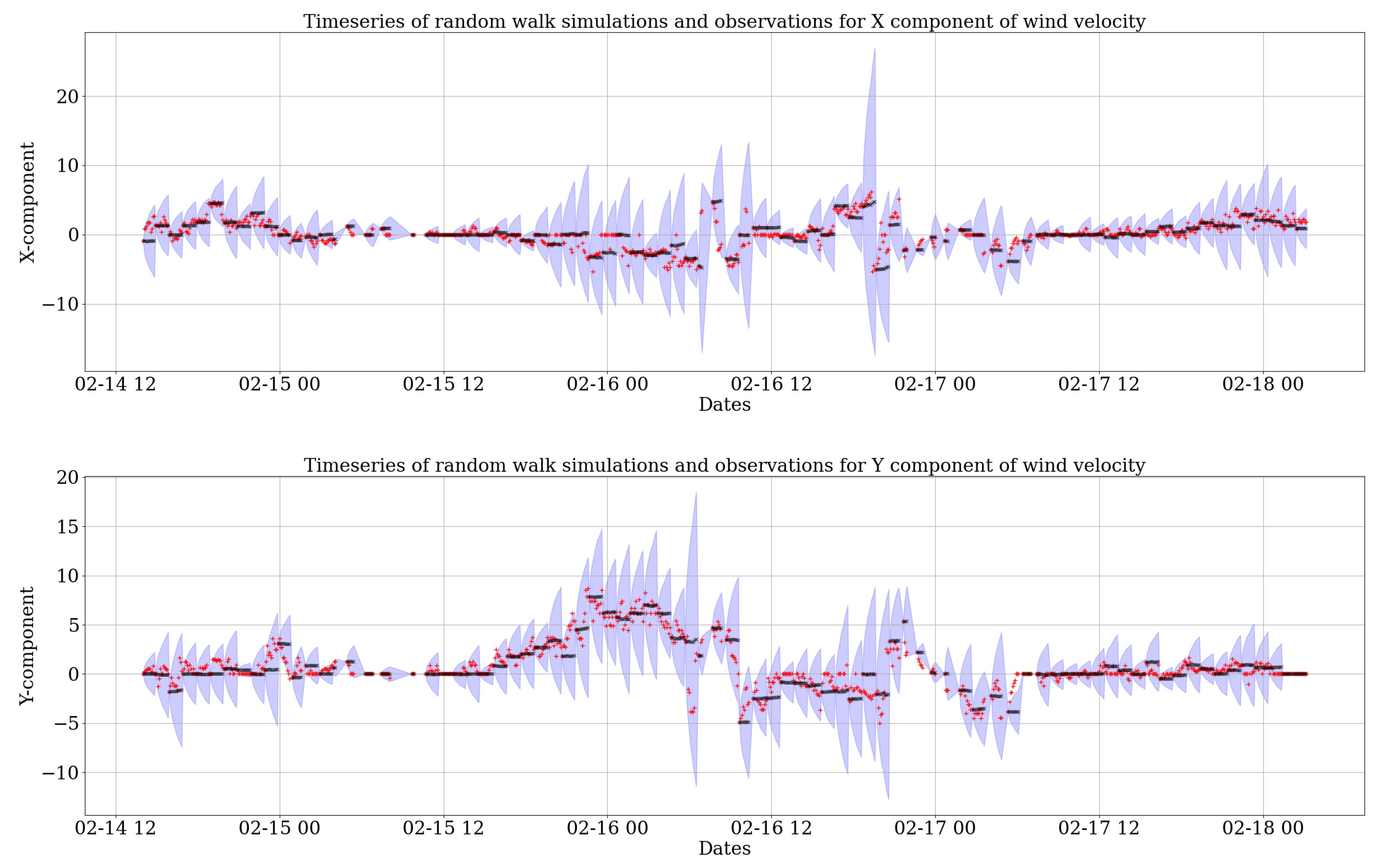
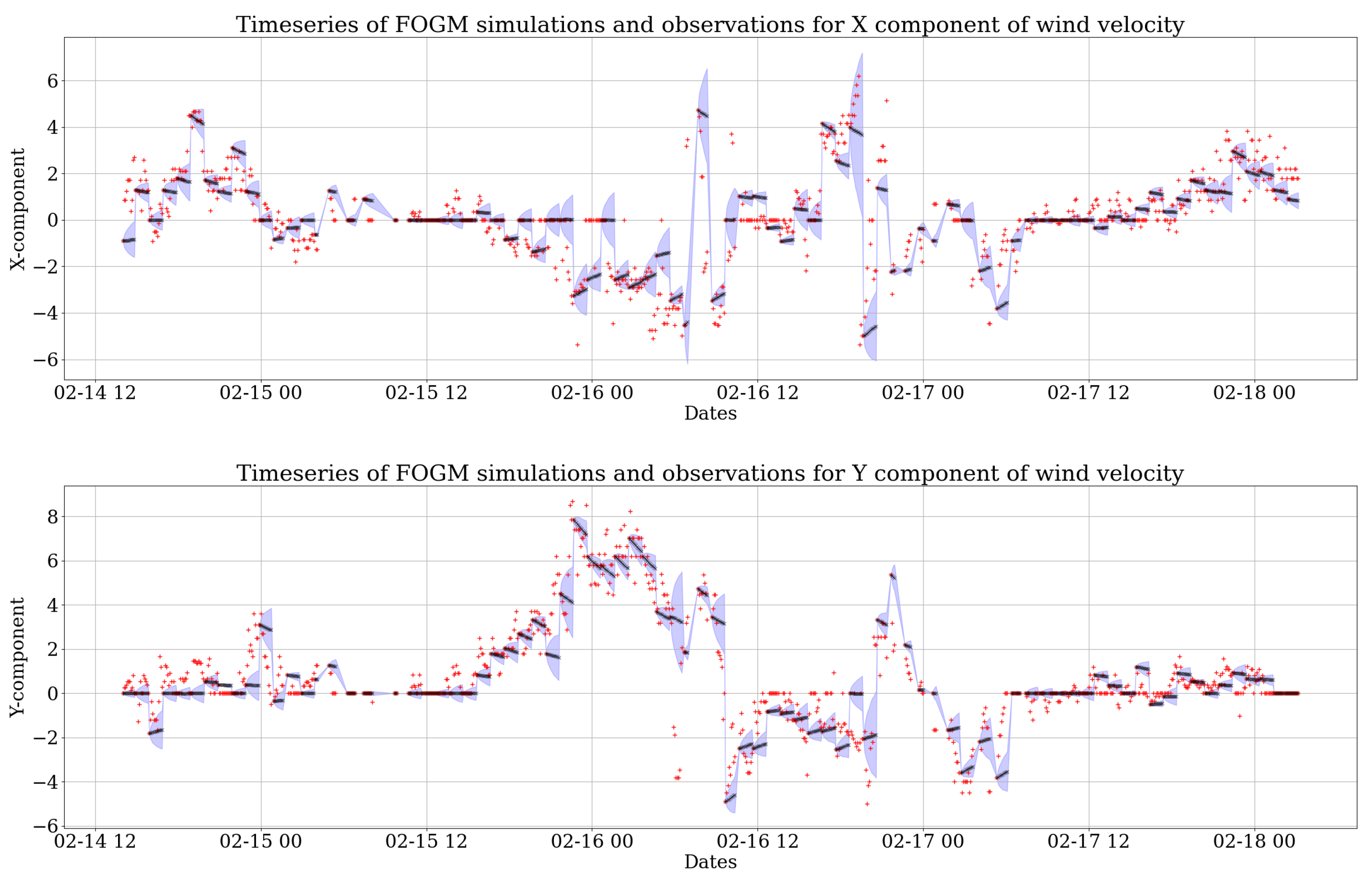
The resulting predictions for 3 days (14–18 February 2014) can be seen in two sets of time series in
Figure 2 and
Figure 3. For each simulation, 1000 realizations were computed. Then, the mean of all of these realizations was compared to the observations to assess how well the model fits the recorded wind data.
Figure 2 shows the resultant components of wind velocity predicted by the random walk process. The
prediction bands of the 1000 realizations in blue show where one expects the simulated data to lie. The black dots give the mean of the 1000 realizations at each time step. It is clear that the mean prediction (black) is very close to the red stars representing the wind velocity observations. Similarly,
Figure 3 shows the predictions from the
fogm model. By comparing
Figure 2 and
Figure 3, it is clear that the variability created by the random walk model is larger than the
fogm process. This is due to the fact that
fogm is a mean-reverting process, which is always naturally bounded and maintains the data around a value, while the prediction band of the random walk simulation tends to cover a higher scatter. However, the mean of 1000 realizations of both stochastic processes (black dots in
Figure 2 and
Figure 3) behave very similarly to the observations of each wind component and also each other.
An evaluation of both the stochastic wind models was performed for the collected data from all 11 weather stations, which resulted in very similar outcomes. In general, the results show that the fogm process gives smaller uncertainties for wind modeling compared to the random walk process. The prediction bands of the fogm process are also much narrower than the bands of the random walk. This is due to the fact that the different simulations of the fogm process are much closer to each other compared to the random walk as a result of the mean-reverting characteristic of the fogm process. However, the means of both stochastic processes exhibit similar behavior and fit very well the observed wind data. This will be further assessed by validating the stochastic wind models in the next section.
3.3. Validation of Estimated Noises for Data Collected from Weather Stations
The simulations were evaluated using the root mean square error (
rmse). If
represents the data predicted using a stochastic process model and
represents the observed data, then the
rmse is calculated as
where
rmse is calculated for the simulations described in the previous section using both the random walk and
fogm processes for all 11 weather stations. For every hourly interval, the corresponding estimated process noise is applied to predict the wind components; then, the
rmse is calculated for that hourly duration. The average of all calculated
rmse for all time intervals was then calculated as the
rmse of the predicted data for each weather station. Additionally, for the sake of the validation of the process noises, the calibrated process noises from each weather station were implemented to model the data for every other station, and, again, the
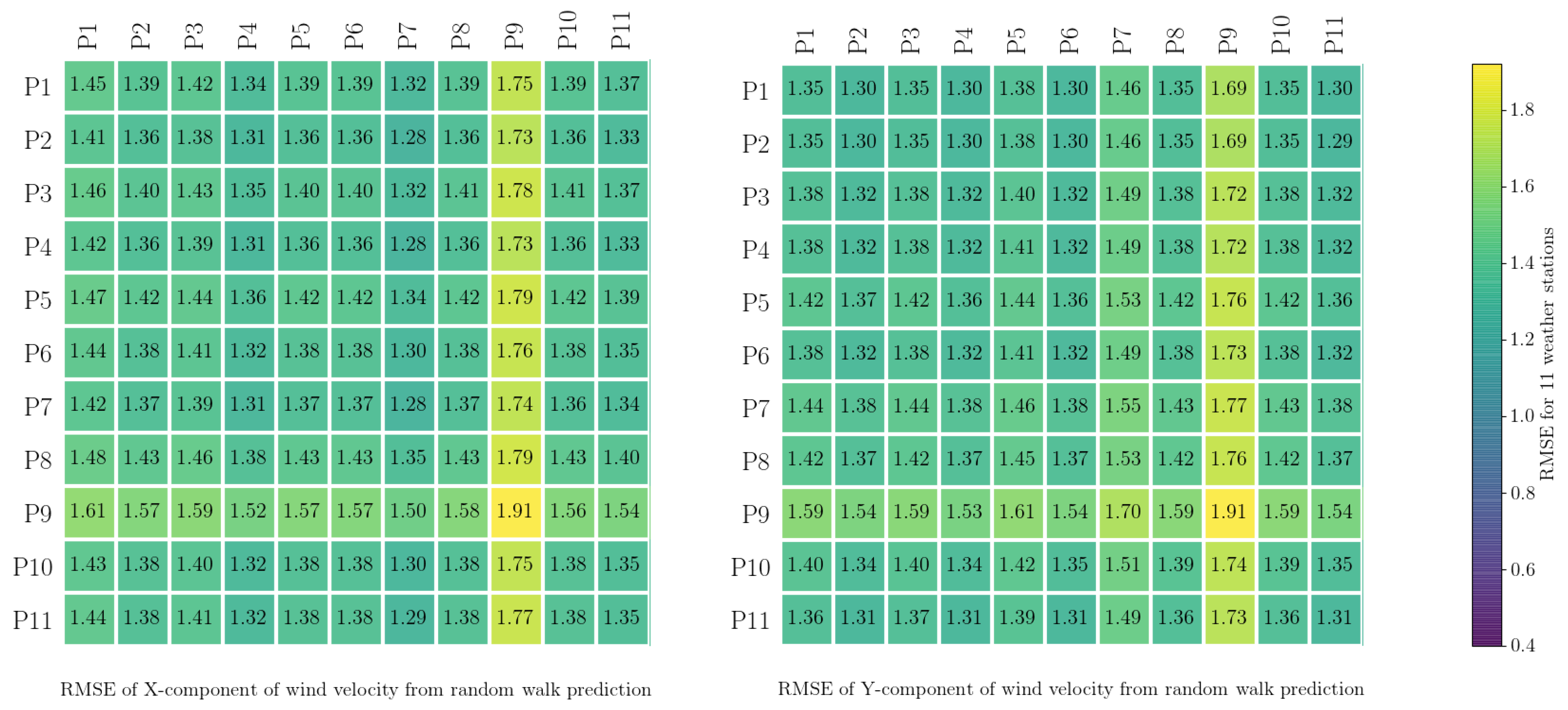
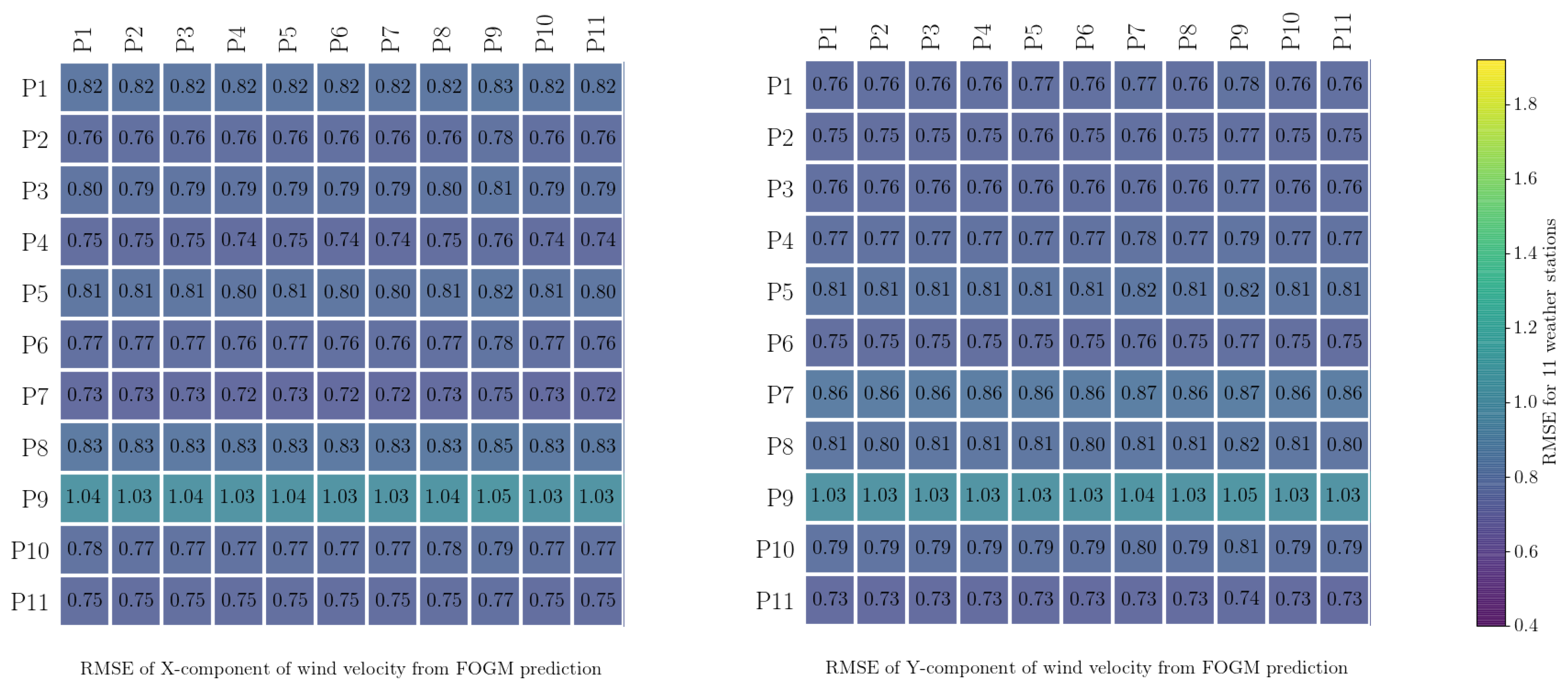
rmse was calculated for each station to understand how valid these estimated process noises were for different spatial positions. The results are presented in
Figure 4 and
Figure 5. From
Figure 4 and
Figure 5, it can be seen that the
rmse from applying the process noises estimated from a particular station to other stations is not generally much different from the
rmse for that particular station. For example, the
rmse of the predicted
x-component at station
paw1 (
p1), resulting from the estimated
fogm process noise for the same station, is about
, whereas using the same process noise for all the other stations results in a similar range for
rmse. This shows that, for this case study, the estimated process noise from the data recorded by any particular weather station is similar to all the other stations. This is as it should be, as all of the weather stations were in close proximity to each other and so were sampling very similar local wind conditions.
The calculated
rmse for the random walk process (
Figure 4) is, in general, slightly larger than the calculated
rmse for the
fogm process (
Figure 5). In these figures, the results for weather station
p9 stand out slightly, and the reason for this is that the duration of data collection for this station was shorter than for the others, as mentioned in
Section 2.1.
The results of the stochastic wind simulations in
Figure 2 and
Figure 3 and the calculated
rmse values in
Figure 4 and
Figure 5 show that the
fogm model produces predictions closer to the observed data when compared to the Wiener model and considering each and every realization of the simulations. The reason is that the
fogm process is a mean-reverting process, so it is naturally bounded and more confined, whereas the Wiener process tends to fluctuate more widely because of its unrestrained variance.
3.4. Comparison of the Stochastic Simulation Distributions
In order to assess the similarity between the distributions of the stochastic wind simulations and the wind observations, Quantile-Quantile (
q-q) plots are used.
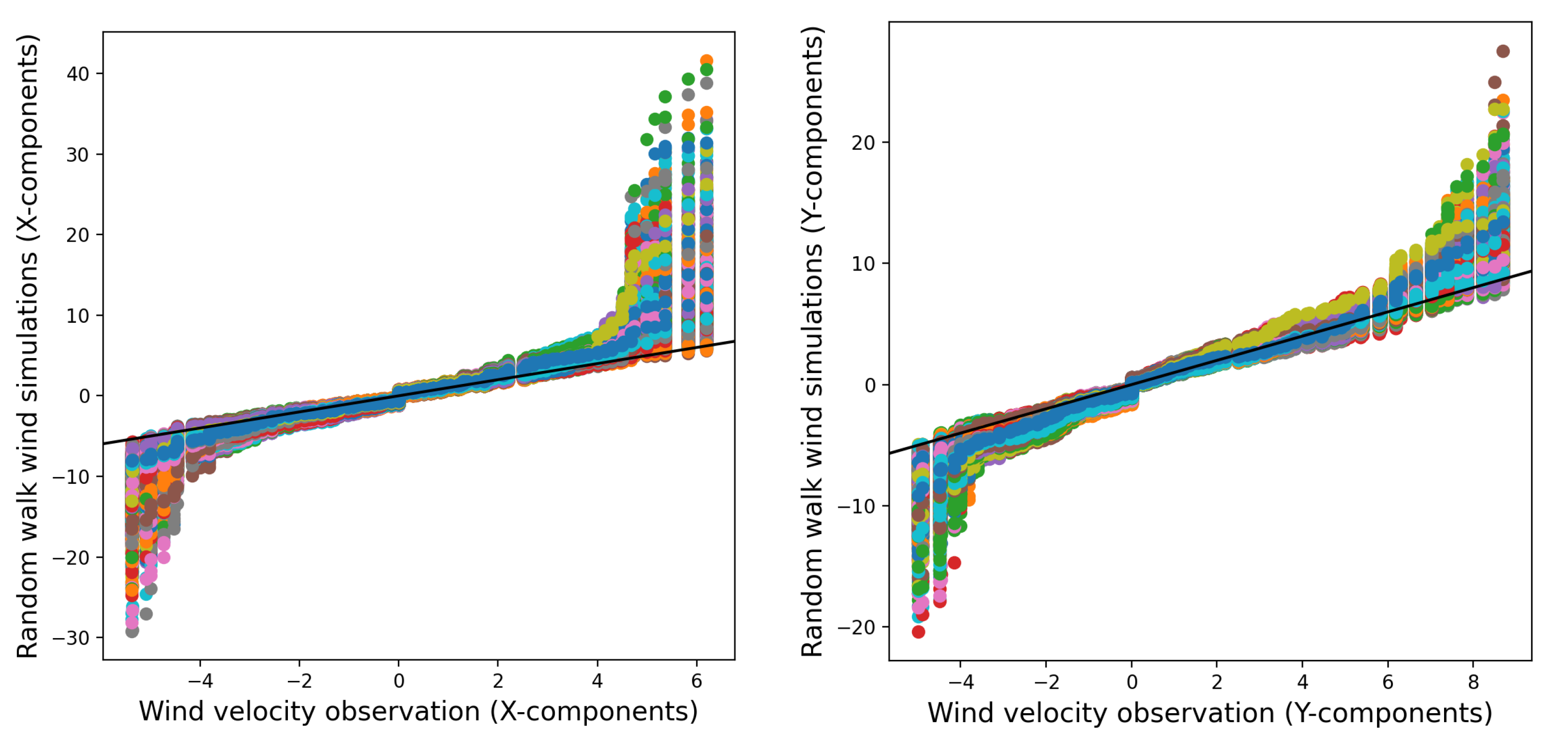
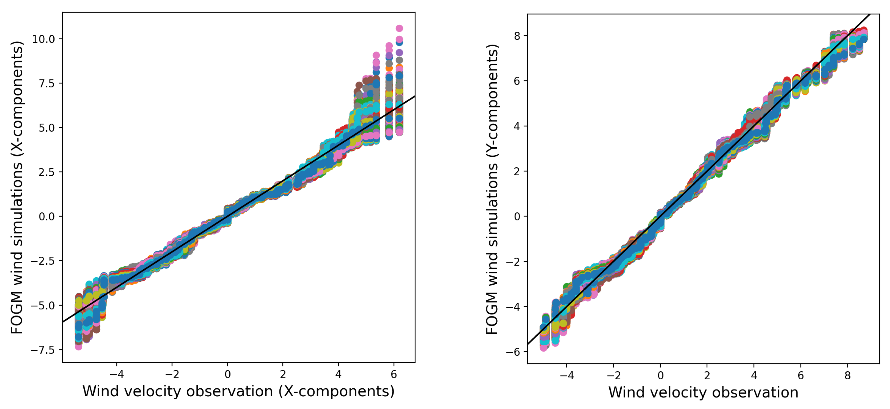
Figure 6 and
Figure 7 use
q-q plots to compare 1000 simulated wind data points from two models from real wind observations. The models include a random walk process for the wind velocity components (
x and
y) and a
fogm process. The comparison helps assess how closely the models’ distributions match the observed data. The simulations are based on estimated process noises, and all data are taken from
paw1 over a 3-day period (14–18 February 2014).
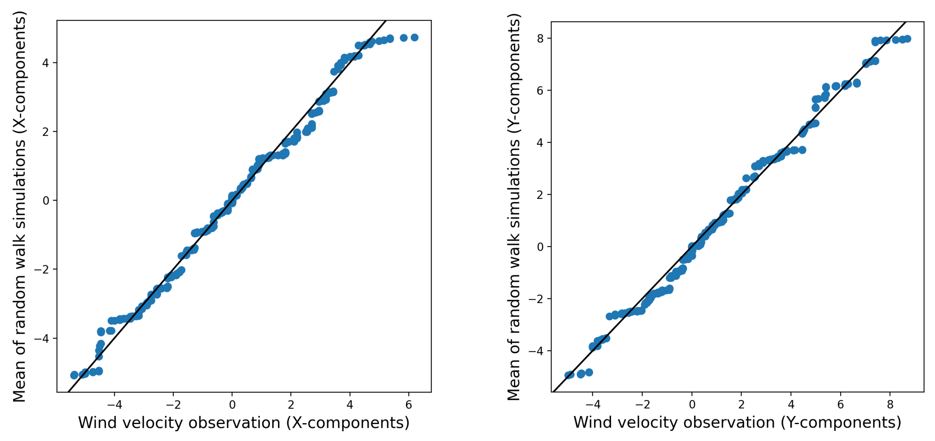
Figure 6 reveals that the random walk simulations exhibit fat tails, indicating greater variability and possible disparities in the extreme values when compared to the distribution seen in the wind observations. However, in
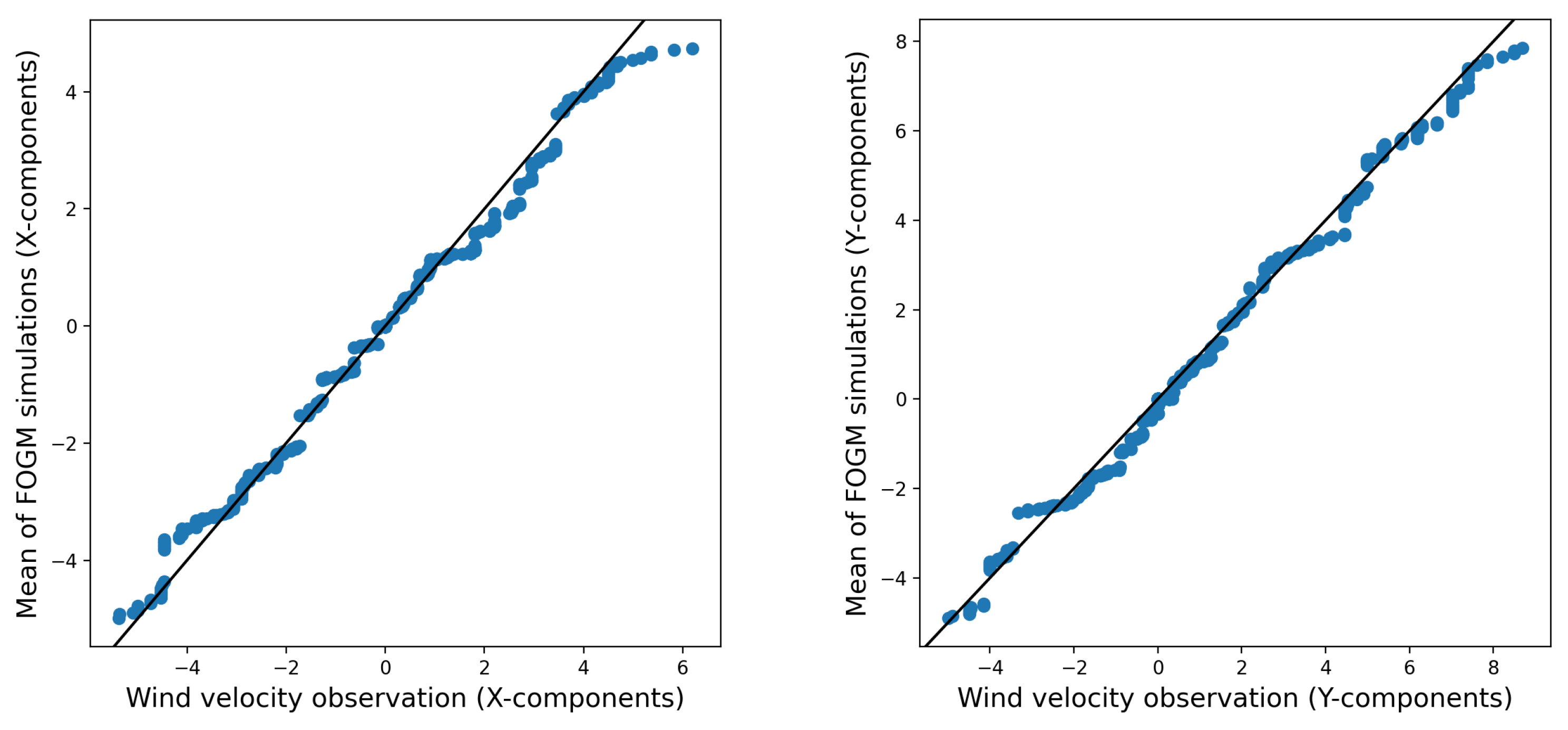
Figure 8, which depicts the average of 1000 realizations of the random walk simulations, these fat tails are less evident. The mean of the simulations seems to closely correspond to the distribution of the observed wind data. This suggests that the random walk model accurately captures the central tendencies and general patterns of wind behavior.
Conversely, the average of 1000 realizations from the
fogm process behaves in a very similar manner to the average of 1000 realizations from the random walk simulation. Additionally, both averages closely align with the wind observations (as shown in
Figure 8 and
Figure 9). This indicates that although the
fogm process generally produces less variation among different simulations and generates values that are nearer to the observed data compared to the random walk simulation (see
Figure 7), the means of the realizations for both stochastic processes are similar and closely resemble the observed data.
It is important to note, however, that obtaining a sufficient number of realizations to accurately capture the average outcomes can be computationally demanding and time-intensive. This aspect provides the fogm process with an advantage over the random walk process.
4. Fire Simulation
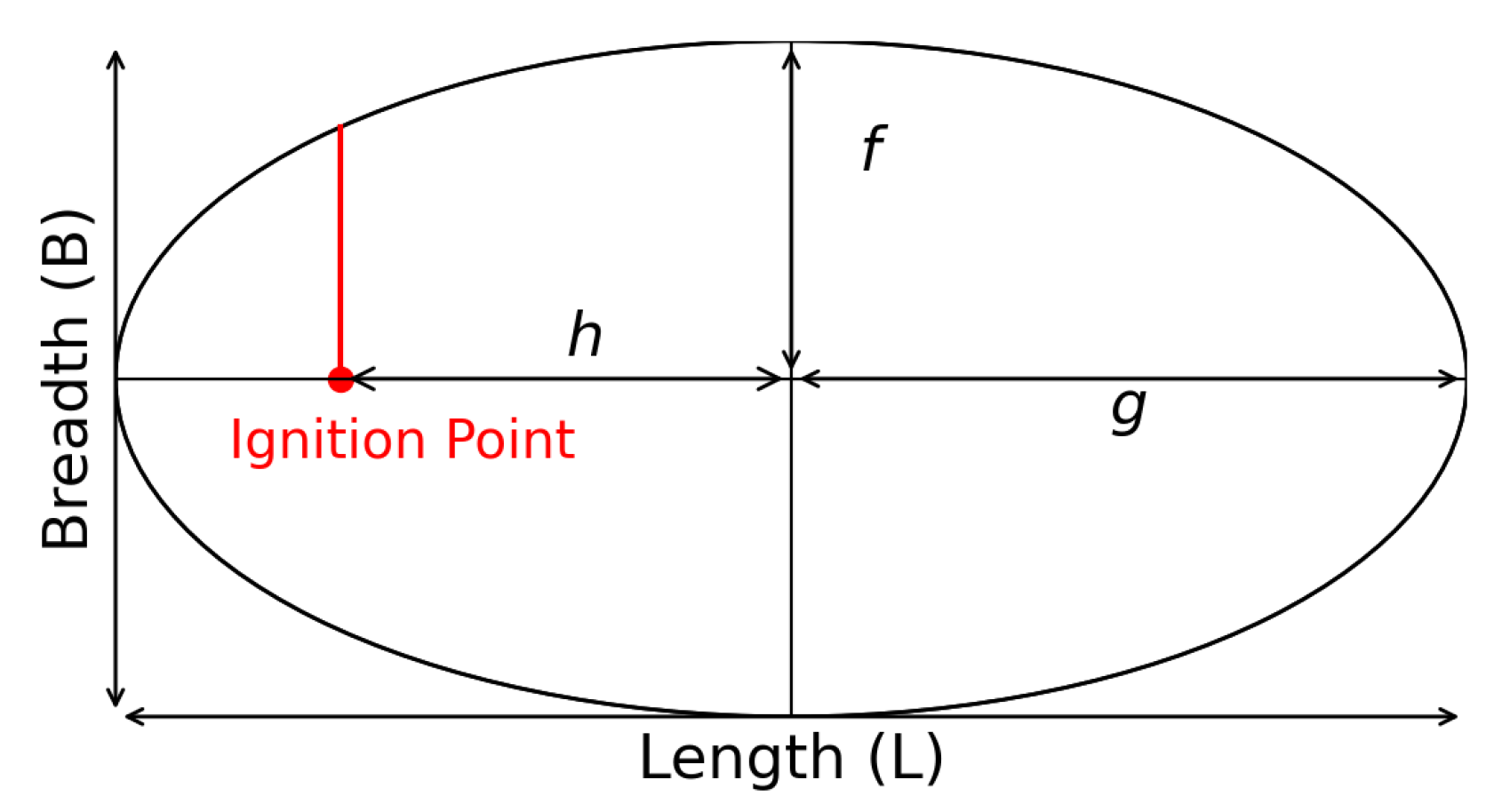
Normally, in rate-of-fire spread simulations, the fire perimeter in two-dimensional space can be modeled based on an elliptic Huygen principle [
14]. We employ such a model here, with shape parameters
f,
g, and
h, as depicted in
Figure 10.
The model describes a fire moving with a speed determined by the wind, which is related to the length-to-breadth ratio,
, of the elliptic stencil [
45]. The spread of the elliptical fire in this model can be described as a normal flow, with the speed given by Robert et al. [
42]:
where
is the unit normal vector to the fire perimeter, and
is the wind direction vector, and
with the head-to-back fire rate-of-spread ratio,
, given by
In order to implement the calibrated stochastic wind models in a fire spread model, the
spark fire spread simulator is used. In this framework, the elliptical fire model can be applied, as well as other deterministic models where the growth of the fire front can be calculated by tracking the distance between the points on the front and the points in a specific domain using the level set method [
46]. The level set method uses the signed distance
as the level set function of a closed curve, which is the fire perimeter; if a point is inside the curve, the signed distance function is negative (
); if it is outside the curve, the function is positive (
); otherwise, the function is zero, which means that the point is located on the boundary of the curve (
). The zero-level set at each time step represents the new fire front at that time step. In other words, the
spark framework is able to track the outward evolution of the fire front, with the speed,
s, at each point on the fire boundary given using the following equation for the level set function:
Wind is an important factor in the spark framework. The fire simulator tracks the direction of fire growth with respect to the wind vector, which can potentially change the direction and the wind speed of the fire, which affects the dimensional parameters of the elliptical stencil via the length-to-breath ratio (stronger winds correspond to a larger length-to-breadth ratio).
In order to integrate the newly introduced stochastic wind model into the
spark solver and adjust the wind components stochastically, the stochastic wind models have been integrated into the level set solver. Subsequently, the
spark solver gains access to and utilizes these models within the advection model. This facilitates the dynamic and stochastic modification of the
advect-x and
advect-y components, ensuring that the variability of the wind is adequately accounted for during the simulation. The script demonstrates how to pass the random walk wind model to the solver.
Figure 11 displays a comparison between the deterministic fire spread model without the implemented stochastic wind models and the fire model with the implemented FOGM wind model, which updates both wind vector components at each time step. The natural variability of wind components throughout the fire simulation is clearly noticeable.
config = {
‘‘resolution’’: 1.0,
‘‘advectionScript’’: ’’’
advect_x = sqrt(dt)∗0.03∗randomNormal(0,1);
advect_y = sqrt(dt)∗0.03∗randomNormal(0,1);’’’
... #buildScript and initialisations if it is needed
}
solver = LevelSet()
solver.init(json.dumps(config), v, inputVariables = variables)
...
The stochastic nature of the wind models presented in this study gives variability in the results of the fire spread simulations, so every realization of the same simulation represents a different fire front. In order to visualize the different possibilities of stochastic wind models, each of the simulations was run 1000 times. The fire spread simulations are executed using various integrated wind models, including ensemble-deterministic, the
fogm process, and the random walk process; the estimated statistics from the
paw stations are utilized, as shown in
Table 3. Besides applying probabilistic approaches to capture the intrinsic uncertainty in wildfire spread, probability maps [
22] can be useful aids in visualizing the possible scenarios of burnt and unburnt regions. The fire spread simulations in
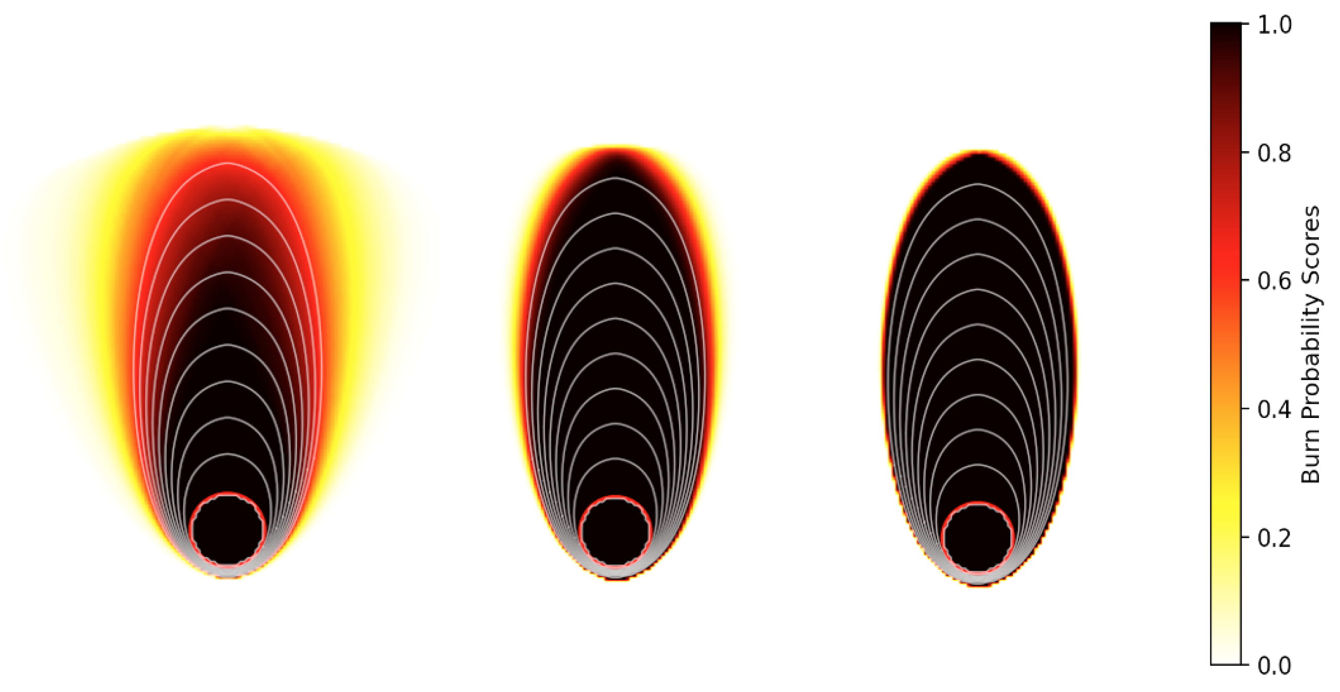
spark, coupled with the different stochastic wind models, are visualized by burn probability maps displayed in
Figure 12. Darker colors show the locations that have higher burn probability scores in comparison with the lighter colors, which are less likely to burn.
Figure 12 shows three different fire scenarios simulated by different probabilistic wind models, including a deterministic ensemble (with distributed inputs generated by a normal distribution, with estimated mean and variance from the observed data), the random walk process, and the
fogm process. In general, the stochastic approaches present a smaller range of uncertainty related to the wind vector; the regions with darker colors and the higher burn probabilities are larger for boththe random walk and
fogm processes when compared to the ensemble simulation on the left side of
Figure 12. Additionally, the implemented
fogm process in the fire simulation shows less uncertainty compared to the random walk simulation, as would be expected from previous observations.
5. Discussion
Incorporating time series derived from stochastic wind velocity simulations has the potential to extend the capability of bushfire modeling to capture the intrinsic stochastic variation of fire propagation. Both stochastic wind models considered here supported this capability, even though they exhibited slightly different results. The resulting fire simulations provide more useful and well-informed predictions compared to the deterministic ensemble simulations in terms of risk assessment. The time series of the ensemble of the random walk model follows the observed variability in the wind components over time with a broader band for the prediction compared to the time series of the ensemble
fogm prediction. Although the distribution of every realization might not fit the observed values very well in
Figure 6 and
Figure 7, the average of the different realizations gives predictions that are very close to the wind observations in
Figure 8 and
Figure 9. The fat-tailed
q-q plots for the random walk simulations confirm this observation. The random walk model is able to introduce uncertainty into the wind factor for fire spread simulation, with a narrower uncertainty band for the probability of burning compared to the deterministic ensemble model.
On the other hand, the individual realizations of the ensemble
fogm model produce very similar wind predictions to the wind observations, which can be observed in the time series of the simulations, as well as the resultant thin tail
q-q plots. Even though the individual realizations of the random walk model sometimes produce simulations less similar to the observed data than the
fogm model, the average of all the ensemble members from both models shows similar outcomes that represent the observed data very well (shown in
Figure 8 and
Figure 9). Implementing the
fogm wind model in
spark exhibits an even narrower band of uncertainty in the burned probability map compared to the fire spread models for both the implemented random walk wind prediction and the deterministic ensemble.
The information conveyed from different burn probability maps has the potential to better inform the decision-making of fire management personnel, as they provide an estimate of the relative likelihood of different regions being burnt in a particular fire event. Implementing the deterministic and stochastic wind models with different associated levels of uncertainty provides insights into the different levels of risk that apply in various forecast scenarios. These insights can then assist expert fire behavior analysts in making predictions about likely fire progression and the associated decisions related to resource allocation or public evacuation. Future work will examine how to best capture the intrinsic variability of real wildfires, as the over-estimation of fire propagation can result in the needless allocation of resources or public evacuations, whereas the under-estimation of fire propagation can have far more dire consequences. Overall, it is important to employ models that more faithfully and accurately account for the processes that underpin the intrinsic variability of fire spreading and better capture the many uncertainties that make wildfire spread prediction such a challenging task.
The data used in this study were collected from a particular location characterized as flat grassland, which may not be representative of more general environments where fires may burn. The uniqueness of the data originating from multiple stations in close proximity to the same location is exceptionally rare. As such, the estimated process noises may not be applicable for other locations that do not match the particular wind characteristics considered here. Applying stochastic wind models as part of bushfire simulations in different locations—especially those in complex forested terrain—would require similar but separate analyses to determine the process noises and the validity of the stochastic wind models. This would be an essential requirement in extending the model across different geographical conditions. Nevertheless, the process noise levels estimated in this study can provide a good indication for realistic noise levels to be used when implementing stochastic processes to simulate wind data.
