The Influence of pH Dynamics on Modeled Ammonia Emission Patterns of a Naturally Ventilated Dairy Cattle Building

Abstract

Ammonia emission rates from naturally ventilated livestock housing systems can be estimated in multiple ways. By coupling different modeling approaches towards a semi-mechanistic barn-scale ammonia emission model, we investigated the influence of urine puddle pH dynamics on the (sub)daily and seasonal pattern of ammonia emissions. We compared the simulated ammonia emission patterns using about ten months of on-farm measurements obtained from a naturally ventilated dairy cattle building with a scraped solid floor in Northern Germany. The dataset included gas concentration measurements as well as wind data (ranging from 0 m s${}^{-1}$ to about 8.6 m s${}^{-1}$) and air temperature data (ranging from about −4 ${}^{\circ }$C to about 32 ${}^{\circ }$C), the average number of housed cows (about 380) and information on the average cow mass (about 700 kg). In addition, the average dry matter intake, total gross energy intake and nitrogen intake were used to model the ammonia emission potential. In the emission modeling, we considered two potential types of pH dynamics in the urine puddles: a saturating scenario and a peaking scenario. For both of them, 21 different combinations of initial pH and maximum pH were considered within a range of 6.5 to 11. We showed that the non-linear interaction of the puddle pH and temperature caused specific emission patterns, where the degree of influence of the two parameters changed over the course of the emission process. Low initial pH values together with high asymptotic pH values were associated with the largest emissions. Considering the same asymptotic pH value, the higher the initial pH value, the lower the observed emissions; especially when assuming peak pH dynamics, the emission values were significantly lower. In natural pH settings (i.e., low to intermediate initial pH and intermediate asymptotic pH), the winter emissions were considerably lower than the summer emissions (i.e., the winter emission was about half of the summer emission, as observed in the on-farm studies). In contrast, artificial pH settings with high pH values led to markedly lower emissions in the summer (i.e., the summer emission was about the same as winter emission), reducing the total annual emission value. Our sensitivity study indicated that the urine puddle alkalizing dynamics play a key role in the overall emission model accuracy in order to capture seasonal and diurnal variability of the ammonia emission of naturally ventilated dairy cattle barns in mechanistic modeling approaches. Thus, future studies should investigate the range of pH dynamics that naturally occur in urine puddles in cattle barns depending on the flooring material, the entry of litter or feed leftovers, the cleaning and cooling system (e.g., in terms of use of water) and so on in order to further refine the emission model.

1. Introduction

Ammonia (NH${}_3$) is a short-living atmospheric tracer gas that affects the environment, climate and health of animals and humans in multiple ways. It forms chemical compounds that acidify soil and water, affecting plant cover and biodiversity. In addition, microbial oxidation of NH${}_3$ to nitrite is associated with the production of nitrous oxide, which is a strong greenhouse gas with a long atmospheric residence time [1]. Moreover, NH${}_3$ contributes to the formation of secondary particulate matter, which impairs the respiratory and cardiovascular systems of animals and humans [2].

Having 80% to 90% of the global emissions, agriculture is by far the largest emitter of NH${}_3$ [3]. In Europe, more than 90% of NH${}_3$ emissions originate from agricultural production, about 22% of which are associated with the housing and manure management of cattle [4]. Animal housing NH${}_3$ originates almost exclusively from chemical reactions on the floors of barns or exercise yards and in (liquid) manure storage. The reaction speed, and consequently, the emission value per time unit, are both particularly high when urine and feces come together due to enzymatic activity. The enzyme urease, which is contained in the feces, decomposes uric acid into carbamic acid and NH${}_3$. The carbamic acid is unstable at temperatures above −23 ${}^{\circ }$C and spontanously decomposes into NH${}_3$ and carbon dioxide (CO${}_2$) [5]. Solved in water, the NH${}_3$ will be partly converted to ammonium (NH${}_4$) ions, where only the NH${}_3$ will evaporate. Depending on the actual environmental conditions (particularly the pH and temperature of the liquid), there will be a defined equilibrium between NH${}_3$ and NH${}_4$ [6]. In consequence, the local emission source strength of NH${}_3$ depends on the available nitrogen, the liquid’s pH and temperature and on the near-surface wind speed. It is a result of the complex interplay of the dissociative, enzymatic and evaporative processes (cf. [7]).

Because the emission value of an individual husbandry system is influenced by multiple factors, a detailed acquisition of emission data requires extensive resource usage for on-farm measurements, whereas it is still associated with large uncertainty. The literature suggests that a high variation of both NH${}_3$ concentration and emissions are associated with the specificity of measurements in the buildings [8]. Direct measurements of gas concentrations and emissions are impaired by spatially inhomogeneous and temporally fluctuating dilution rates as a result of the complex air flow pattern [9,10]. Moreover, the high variation in both NH${}_3$ concentration and emissions can be associated with the specificity of measurements in the buildings [8]. In consequence, different modeling approaches have been developed over the past decades to make expensive, overarching measurement campaigns obsolete in the future. These methods include the balancing of nutrition and excretion, reaction kinetics models for individual urine puddles and storage tanks and gas dispersion modeling (e.g., [11,12,13,14,15]). All of them represent crucial aspects of the emission process and focus on different spatial and/or temporal scales. In order to draw conclusions on whole housing systems, the models typically rely on either complex measurements or default values. Many of the input values can only be assessed with large uncertainty [16]. It has been shown that this issue can be minimized when different (semi-)mechanistic modeling approaches are coupled [7].

Snoek et al. (2014) reported that, with regard to the reaction kinetics of urine puddles, the actual sensitivity of the model on the input variables depends on the considered timeframe [16]. In their study, five variables turned out to be particularly important for the global model sensitivity, namely the pH value, puddle depth, initial urea concentration, puddle area and puddle temperature.

For the pH value of cattle urine, which (as one of the key influencing factors) we will focus on in the present sensitivity study, a large range of values is reported in the literature. The reported measurements ranged from below 6 to 8.6 (for fresh urine) or even 9.3 (for about 1 h old urine) [17,18,19]. Healthy cow urine pH typically ranges between 7.4 and 8.4 with seasonal variations [20].

Studies by Hempel et al. (2022) came to the conclusion that the predicted emission pattern using a nested reaction kinetics model was particularly sensitive on the assumed pH dynamics in the liquid during the emission process [7,21]. It was further observed that there was some season-dependent shaping for this effect [21]. Moreover, it was shown that the interaction between urine puddles and ambient temperature affected the emission rates, leading to an overestimation of NH${}_3$ emissions [22]. This was also highlighted by a meta-analysis showing that urine puddles together with seasonal temperature had a more significant effect on NH${}_3$ emissions than housing factors in commercial barns [23].

However, little is known so far about the actual temporal evolution of the pH in urine puddles. There are a few studies indicating that the pH of fresh manure in the first hour(s) quickly increases, then saturates and finally tends to decrease again [5,24,25]. Snoek et al. mentioned a reference value of pH = 9.4, which is used to model NH${}_3$ emissions from concrete slatted floors in the Netherlands, while their own pH measurements showed a pH increase up to 9.0 for concrete and asphalt floor [18]. An earlier study by Sommer et al. under lab conditions reported a strong increase in the pH of cattle slurry at 8 h, followed by a phase of a nearly constant pH and a decline after about 20 h (faster at higher temperatures than at lower temperatures) [26]. The direction of the pH change was associated with the ratio of total inorganic carbon to total ammoniacal nitrogen. It can be expected that similar temporal patterns will also occur in emitting urine puddles. The influencing factors on and the resulting modulations of the temporal dynamics of the pH are, however, not well described in the literature, and the potential influencing factors are barely measured for on-farm conditions, respectively.

Our study aimed to systematically review the effect of different settings of initial and asymptotic pH dynamics on the projection of the long-term NH${}_3$ emission pattern of a naturally ventilated dairy cattle building with solid floors. We hypothesized that the dynamics of the pH during the emission process in interaction with the puddle temperature cause specific emission patterns. In consequence, even with the same initial or average pH value, the average annual emission can vary. Thus, considering the change of urine puddle pH over time when mechanistic modeling is used to assess the potential NH${}_3$ emissions of a facility will contribute to the improvement of digital models that describe the complex interactions between the design and management of livestock housing facilities, the ambient climate conditions and the actual NH${}_3$ emissions.

2. Materials and Methods

2.1. Farm Site and Data Collection

A naturally ventilated dairy barn in Northern Germany was considered as the reference case. The internal room volume of the building was about 25,000 m${}^3$. Natural ventilation was facilitated via the two widely open long sidewalls; gates, doors and space boards in the gable walls; and a 0.5 m ridge slot. Four temperature-controlled operating ceiling fans further supported ventilation. The building has a gable height of about 11 m, a side wall height of about 4 m and a floor area of 96 m by 34 m, consisting of four compartments. Compartments I and II housed groups of about 120 cows, and compartments III and IV housed groups of about 70 cows (cf. Figure 1). The average body mass of the cows was about 700 kg. The cows went to the milking house three times a day (approx. at 6:00 a.m., 2:00 p.m. and 10:00 p.m.) in groups for about an hour each time. Feed was delivered at about 06:45 a.m. and 10:30 a.m. as a total mixed ratio. The solid concrete floors of the alleys were cleaned using automatic scrapers every 1.5 h. We measured the concentrations of CO${}_2$ and NH${}_3$ over 10 months using a two Fourier transform infrared (FTIR) spectrometer (Gasmet CX4000, Gasmet Technologies Inc., Karlsruhe, Germany). We used ten orificed Teflon sampling lines (orifice distances of about 10 m). One of the measuring lines was mounted below the ridge, and the other lines were approximately at the 3 m height. The air temperature was measured with an EasyLog USB 2+ sensor (Lascar Electronics Inc., Whiteparish, UK) in the vicinity of the building. Inflow velocity was measured using a Windmaster Pro ultrasonic anemometer (Gill Instruments Limited, Lymington, Hampshire, UK) mounted at the ridge of the building. Near-surface wind speed was estimated based on computational fluid dynamics simulations neglecting the supporting fan ventilation, the details of which can be found in [27]. Compartment-related stocking density, average animal mass, milk yield and composition, dry matter intake (DMI) and chemical composition of the feed were provided by the farm management. A summary of the inter-group variation in the main descriptive variables is provided in

Table 1. Summary of farm data. The group numbers refer to the four compartments of the building, which accommodated cows in different lactation states (cf. Figure 1). Number of cows and dry matter intake were obtained as average values from herd management. Air temperature and inflow values were estimated from measurements, and the remaining quantities were estimated from simulations of submodels (i.e., the digestion and excretion model and the fluid dynamical airflow model).

Group	I	II	III	IV
Average number of cows	120	120	70	70
Dry matter intake in g d${}^{-1}$	24,078	23,897	22,485	20,451
Total gross energy intake in MJ d${}^{-1}$	444.094	449.093	423.297	389.725
Fraction of ash	81	81	77	81
Nitrogen intake in g N d${}^{-1}$	642.9	681.9	576.0	527.8
Milk N per growth N	213.2	207.8	181.2	186.5
Milk (kg Fat- and protein-corrected milk d${}^{-1}$)	40.7	39.6	34.6	35.6
Total excreted nitrogen in g N d${}^{-1}$	429.7	474.1	394.8	341.3
Total urine nitrogen in g N d${}^{-1}$	239.5	282.0	205.4	171.4
Total fecal nitrogen in g N d${}^{-1}$	190.2	192.1	189.4	169.9
Volume urine in l d${}^{-1}$	46.69	46.98	43.94	40.13
Mean near-surface wind speed in m s${}^{-1}$	1.03 ± 0.54	1.02 ± 0.52	1.07 ± 0.51	1.03 ± 0.57
Max near-surface wind speed in m s${}^{-1}$	2.77	2.72	2.77	3.09
Mean air temperature in ${}^{\circ }$C	10.51 ± 7.13	10.51 ± 7.13	10.51 ± 7.13	10.51 ± 7.13
Min air temperature in ${}^{\circ }$C	−4.30	−4.30	−4.30	−4.30
Max air temperature in ${}^{\circ }$C	32.3	32.3	32.3	32.3
Mean inflow in m s${}^{-1}$	2.01 ± 1.36	2.01 ± 1.36	2.01 ± 1.36	2.01 ± 1.36
Max inflow in m s${}^{-1}$	8.59	8.59	8.59	8.59

.

In addition, on a day in December, the temperature and pH value of twelve urine puddles were measured together with the near-surface air temperature. The puddles were randomly distributed in the barn as shown in Figure 1. For more details about farm site and data collection, we refer to previous publications (e.g., [7]).

2.2. The Nested Model

The barn-scale NH${}_3$ emission model used in this sensitivity study builds on a set of differential equations that describe the change of the total ammoniacal nitrogen (i.e., sum of ammonia and ammonium, TAN) and urea concentration (U) in urine puddles during the release of NH${}_3$ (cf. Equations (1) and (2)).

$$\frac{dU}{dt}=-\frac{c_{1}U}{c_2+U}$$

(1)

$$\frac{dTAN}{dt}=f(pH,v,T)\times \frac{TAN}{d}-2\frac{dU}{dt}$$

(2)

Here, $c_1$ refers to the maximum conversion rate of urea, $c_2$ is the Michaelis constant, d is the puddle depth and f is a function of puddle pH ($pH$), puddle temperature (T) and near-surface wind speed (v), which merges the mass transfer coefficient, ammonia fraction and Henry’s constant. Values for the initial TAN and urea concentration, pH and temperature of the emitting urine puddles, near-surface wind speed, and the effective emission active surface area are required as model inputs. Except for the effective emission active surface area, all of this information is obtained from submodels based on data of feed chemical composition, milk yield and incident wind velocity and air temperature. The effective emission active surface area remains as a tuning parameter in the model. Thus, the overall model is semi-quantitative as it can quantify the ratios of emission values in reaction to varying puddle and wind field features, while the average total emission value is defined by the value of the tuning parameter. Details on the core model and submodels can be found in the literature [7]. In the present study, we considered that urination is uniformly distributed during the day and that urine puddles cool down from body temperature to ambient air temperature following the Newtonian law of cooling [28]. Moreover, a group compartment-specific average near-surface wind speed was considered, which we obtained by downscaling the inflow wind velocity with scaling factors that were derived from computational fluid dynamics simulations [27].

The pH value was determined as a function of the hypothetical values of the initial pH and asymptotic pH of the urine puddles. The change in pH over time was modeled as a superposition of two exponential terms (see Equation (3)) based on the literature [25].

$$p{H}_t=p{H}_f-a_1\times (p{H}_f-p{H}_i)\times e^{(-k_{1}t)}-a_2\times (p{H}_f-p{H}_i)\times e^{(-k_{2}t)}$$

(3)

Here, $p{H}_t$ is the pH value after time t in hours, $p{H}_i$ is the initial pH value, $p{H}_f$ is the final pH value and $k_1$ and $k_2$ are the alkalizing rates. The values of $a_1$ and $a_2$ represent the fraction by which each of the two exponential contribute to the pH value. The first exponential term is describing the fast increase in pH in the beginning of the emission process, while the second is describing the slowing down of the alkalization towards the asymptotic pH. We set $a_1=0.45·(p{H}_f-p{H}_i)$ and $a_2=0.55·(p{H}_f-p{H}_i)$, following the observations made by Snoek et al. [25]. The parameter $k_1$ and $k_2$ were estimated from 12 on-farm samples of urine puddle pH and temperature, which were collected in the barn (cf. Figure 1). They were derived by comparing the measured values with model predictions for a given age of the puddle, permitting $k_1$ to range between $0.5$ and 7 and $k_2$ to range between $0.1$ and 2 (based on the values reported in the study by Snoek et al. [25]). Because the exact age of the measured urine puddles was unknown, first, the age of each puddle was estimated by assuming that all puddles cooled down from 39 ${}^{\circ }$C following the Newtonian law of cooling at approximately the same cooling rate, where a maximum age of one hour was set. The final selected parameter values represent the parameter combination that fits, on average, the best with the 12 measurements given the assumed values $p{H}_i$ and $p{H}_f$.

In this study, the change in pH over time was considered for two options: in the first case, it was assumed that Equation (3) is applicable for the whole 24 h period of model integration per urination event; in the second case, Equation (3) was considered valid only until time $t_{max}$, where after this time, the pH will decrease exponentially again (cf. [5]). This late exponential decay was approximated using Equation (4).

$$\widehat{p{H}_t}=p{H}_t\left[t_{max}\right]+exp(0.005\times (t_{max}-t))$$

(4)

Here, $\widehat{p{H}_t}$ is the pH value at time t and $p{H}_t\left[t_{max}\right]$ is the maximum pH value reached after time $t_{max}$ according to Equation (3). The maximum time for the pH raise was set to $t_{max}=10$ h for this study.

Moreover, two cleaning efficiencies, $c_{eff1}$ and $c_{eff2}$, were considered. The cleaning efficiency is a tuning parameter of the nested model, which represents the fraction of remaining emission active surface area after each scraping event. As scraping involves two contradicting effects, namely the removal of liquid and its smearing on the surface, the joint effect on the emission active surface cannot be directly measured. The first value $c_{eff1}$ was taken from the study where the nested model was originally introduced [7]. It was used to tune the model based on a small subset of emission values in order to achieve the maximum correlation between simulated and measured emissions. This set of input parameters was similarly applied to this study. Particularly, the pH change was considered to follow Equation (3) for the whole duration with $p{H}_i=6.8$ and $p{H}_f=9.2$. The second value of the cleaning efficiency, $c_{eff2}$ in the present study, was selected in such a way that the average simulated emission value for $p{H}_i=7$ and $p{H}_f=9$ was in the same order of magnitude when using Equation (4) as it was in the setup before.

2.3. Emission Value Derivation

In order to derive the emission values from the gas concentration measurements, the outdoor sample line with the lowest CO${}_2$ value was selected to determine the background gas concentrations $CO{2}_{bg}$ and $NH{3}_{bg}$ in the incoming air at each timestamp. The average concentration value of the six sample lines inside the barn at the same timestamp was used to estimate gas concentrations $\overline{CO{2}_{in}}$ and $\overline{NH{3}_{in}}$ in the outgoing air. The ratio of the indoor–outdoor concentration differences of NH${}_3$ and CO${}_2$ was then multiplied with the theoretical CO${}_2$ production rate $P_{CO2}$ to obtain the emission value for the timestamp (cf. Equations (5) and (6)).

$$E=P_{CO2}\frac{\overline{NH{3}_{in}}-NH{3}_{bg}}{\overline{CO{2}_{in}}-CO{2}_{bg}}$$

(5)

$$P_{CO2}=\frac{(1000+4\times (20-T))\times 0.2\times (5.6\times M^{0.75}+22\times Y+1.6\times {10}^{-5}\times D^3)}{1000}$$

(6)

Here, T is the air temperature and M, Y and D are the average mass, milk yield and days of pregnancy of the cows, respectively. The described procedure is known as the CO${}_2$ balance method and is further described, e.g., in [10]. In case of missing or negative gas concentration differences, the timestamp was omitted.

In order to derive theoretical emission values, we varied the initial pH ($p{H}_i$) from 6.5 to 10.5 and the asymptotic pH ($p{H}_f$) from 8 to 11, both in steps of 0.5. Combinations with $p{H}_i\ge p{H}_f$ were omitted in this sensitivity study. For each of the remaining combinations, hourly NH${}_3$ emission values for a period of 302 days were simulated. First, the pH was considered to follow Equation (3) for 24 h while $c_{eff1}=0.415$. Next, the pH was considered to follow Equation (3) for 10 h and then follow Equation (4) while $c_{eff2}=0.380$.

2.4. Data Analysis

The individual emission values and their distributions were compared between the sets obtained for different simulation cases and the set that was derived from gas concentration measurements. In order to evaluate the effect of the pH dynamics on the emission time series, we quantified the deviation between the different simulated emission time series and the experimentally derived time series using the RMSE. In this case, the experimentally derived time series serve as a reference. In addition, we calculated the correlation of the different simulated emission time series with the experimentally derived time series (i.e., with the reference). Note that in this setting, a large deviation or low correlation means that the considered pH dynamics are likely not representative for the actual pH dynamics during the measurements. It does not necessarily mean that the respective pH dynamics cannot occur under any practical conditions.

Besides the comparison of the time series itself, we also considered deviations in the distributions of emission values. Therefore, we compared rank-ordered sets instead of the time series, which is a common procedure used in modeling to identify and correct systematic biases introduced by the model. In this case, the temporal order was neglected, and the focus was purely on the probability distribution. This permits us to reveal relations that are otherwise hidden by temporal fluctuations, but with the cost of losing potential causal relations. The deviation between the differently rank-ordered sets of simulated emissions and the rank-ordered set of experimentally derived emission values was again quantified using the RMSE, where the experimentally obtained data were considered as a reference. In addition, the distributions of all time series values were compared in violin plots. The plots show the median of each set together with the interquartile range and rotated kernel density estimated for the respective set.

Finally, we analyzed the seasonal relative and absolute deviations of the different simulation cases from the respective reference value (i.e., the experimentally derived emission values). Here, seasons were defined as calendar date-based periods: winter (December, January and February), transition (March, April and May) and summer (June, July and August).

3. Results

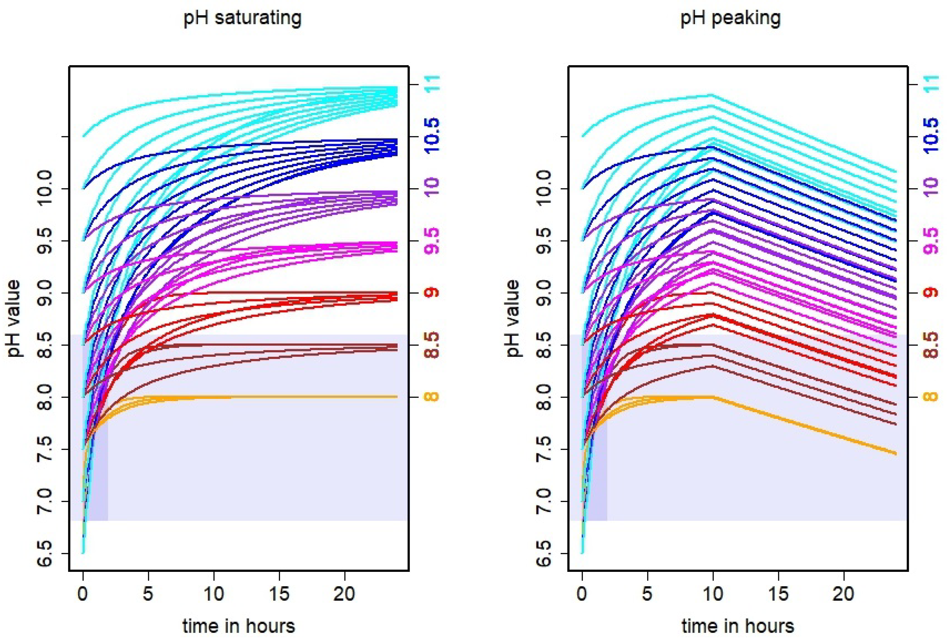
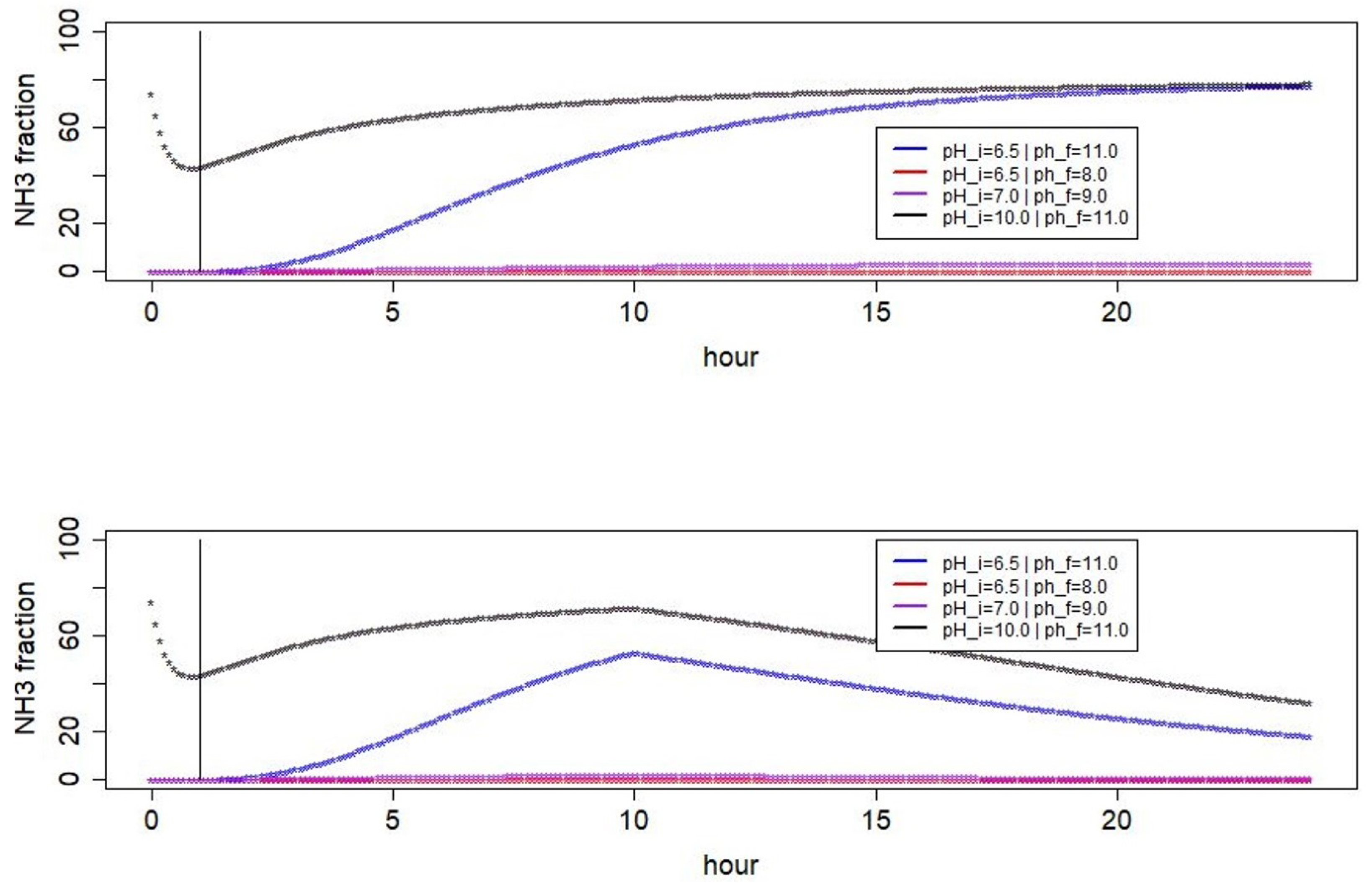
3.1. Simulated pH Dynamics

When varying $p{H}_i$ and $p{H}_f$ and fitting Equation (3) to the 12 puddle samples, we obtained average values for the parameters: $a_1=0.86$, $a_2=1.05$, $k_1$ = 0.81 h${}^{-1}$ and $k_2$ = 0.19 h${}^{-1}$. The actual parameter values for each combination of $p{H}_i$ and $p{H}_f$ are listed in

Table 2. Parameter settings of assumed pH dynamics of urine puddles. The initial pH ($p{H}_i$) and maximum pH ($p{H}_f$) have been preset. The other parameters were derived by fitting the example floor measurements illustrated in Figure 1. Two possible versions of the temporal evolution of pH over time were considered. Those follow Equation (3) for the first 10 h of the biochemical reaction (resulting in $p{H}_t\left[10\right]$). Afterwards, the pH evolution follows either Equation (3) (resulting in $p{H}_t\left[24\right]$ after 24 h) or Equation (4) (resulting in $\widehat{p{H}_t}\left[24\right]$ after 24 h). The table provides a list of assumed and fitted parameters describing the pH dynamics in the individual simulation runs. The unit of parameters $k_1$ and $k_2$ is $h^{-1}$; the other quantities are dimensionless. The resulting pH time series are plotted in Figure 2.

${\mathit{pH}}_{\mathit{i}}$	${\mathit{pH}}_{\mathit{f}}$	${\mathit{a}}_1$	${\mathit{a}}_2$	${\mathit{k}}_1$	${\mathit{k}}_2$	${\mathit{pH}}_{\mathit{t}}\left[10\right]$	${\mathit{pH}}_{\mathit{t}}\left[24\right]$	$\widehat{{\mathit{pH}}_{\mathit{t}}}\left[24\right]$
6.5	8	0.675	0.825	4.54	1.03	8	8	7.46
6.5	8.5	0.9	1.1	1.2	0.76	8.5	8.5	7.92
6.5	9	1.125	1.375	0.72	0.63	9	9	8.39
6.5	9.5	1.35	1.65	1.2	0.18	9.23	9.48	8.6
6.5	10	1.575	1.925	0.9	0.16	9.61	9.96	8.96
6.5	10.5	1.8	2.2	0.8	0.11	9.77	10.34	9.11
6.5	11	2.025	2.475	0.57	0.15	10.44	10.93	9.74
7	8	0.45	0.55	6.33	0.58	8	8	7.46
7	8.5	0.675	0.825	0.72	0.57	8.5	8.5	7.92
7	9	0.9	1.1	0.92	0.16	8.78	8.98	8.18
7	9.5	1.125	1.375	0.54	0.19	9.29	9.49	8.66
7	10	1.35	1.65	0.52	0.1	9.39	9.85	8.75
7	10.5	1.575	1.925	0.5	0.1	9.78	10.33	9.12
7	11	1.8	2.2	0.5	0.1	10.18	10.8	9.49
7.5	8	0.225	0.275	0.69	0.33	7.99	8	7.45
7.5	8.5	0.45	0.55	0.5	0.1	8.29	8.45	7.73
7.5	9	0.675	0.825	0.5	0.1	8.69	8.93	8.1
7.5	9.5	0.9	1.1	0.5	0.1	9.09	9.4	8.47
7.5	10	1.125	1.375	0.5	0.1	9.49	9.88	8.85
7.5	10.5	1.35	1.65	0.5	0.1	9.88	10.35	9.22
7.5	11	1.575	1.925	0.5	0.1	10.28	10.83	9.59
8	8.5	0.225	0.275	0.5	0.1	8.4	8.48	7.83
8	9	0.45	0.55	0.5	0.1	8.79	8.95	8.2
8	9.5	0.675	0.825	0.5	0.1	9.19	9.43	8.57
8	10	0.9	1.1	0.5	0.1	9.59	9.9	8.94
8	10.5	1.125	1.375	0.5	0.1	9.99	10.38	9.31
8	11	1.35	1.65	0.5	0.1	10.38	10.85	9.68
8.5	9	0.225	0.275	0.5	0.1	8.9	8.98	8.3
8.5	9.5	0.45	0.55	0.5	0.1	9.29	9.45	8.67
8.5	10	0.675	0.825	0.5	0.1	9.69	9.93	9.04
8.5	10.5	0.9	1.1	0.5	0.1	10.09	10.4	9.41
8.5	11	1.125	1.375	0.5	0.1	10.49	10.88	9.78
9	9.5	0.225	0.275	0.5	0.1	9.4	9.48	8.76
9	10	0.45	0.55	0.5	0.1	9.79	9.95	9.13
9	10.5	0.675	0.825	0.5	0.1	10.19	10.43	9.5
9	11	0.9	1.1	0.5	0.1	10.59	10.9	9.87
9.5	10	0.225	0.275	0.5	0.1	9.9	9.98	9.23
9.5	10.5	0.45	0.55	0.5	0.1	10.29	10.45	9.6
9.5	11	0.675	0.825	0.5	0.1	10.69	10.93	9.97
10	10.5	0.225	0.275	0.5	0.1	10.4	10.48	9.69
10	11	0.45	0.55	0.5	0.1	10.79	10.95	10.06
10.5	11	0.225	0.275	0.5	0.1	10.9	10.98	10.16

, and the resulting theoretical time series of the pH values are shown in Figure 2. The determined parameter value for $a_1$ varied between $0.225$ and $2.025$ with a median of $0.79$ and a standard deviation of $0.50$. For parameter $a_2$, it varied between $0.275$ and $2.475$ with a median of $0.96$ and a standard deviation of $0.61$. The derived alkalizing rates varied between 0.50 h${}^{-1}$ and 6.33 h${}^{-1}$ for $k_1$ and between 0.10 h${}^{-1}$ and 1.03 h${}^{-1}$ for $k_2$. The associated medians were 0.50 h${}^{-1}$ for $k_1$ and 0.10 h${}^{-1}$ for $k_2$. The associated standard deviations were 1.08 h${}^{-1}$ for $k_1$ and 0.21 h${}^{-1}$ for $k_2$. It turned out that with the estimated parameters, $88\%$ of the simulation cases did not reach the asymptotic pH value after 10 h. After 24 h still, about $86\%$ of the pH values were below the assumed asymptotic pH value.

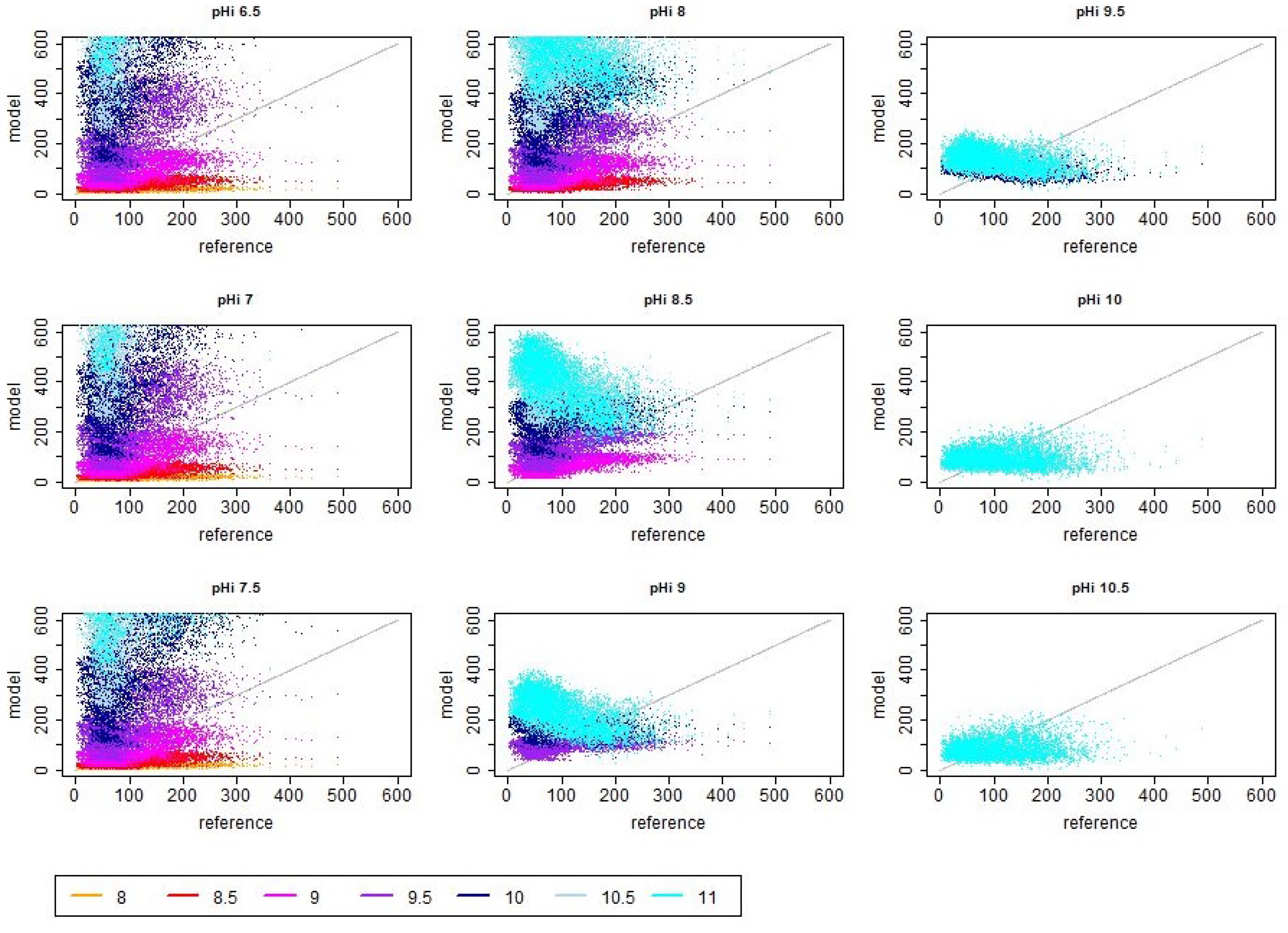
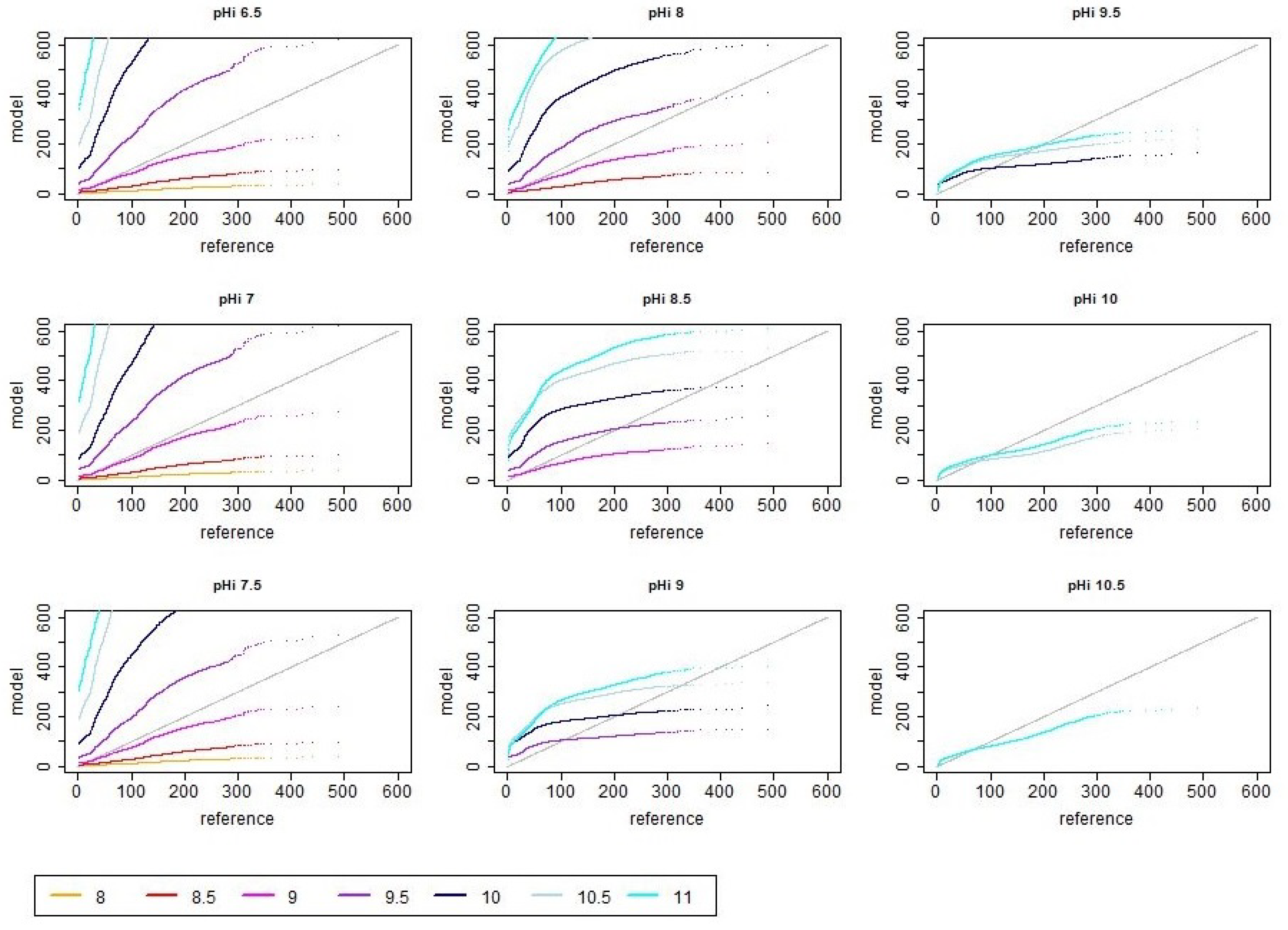
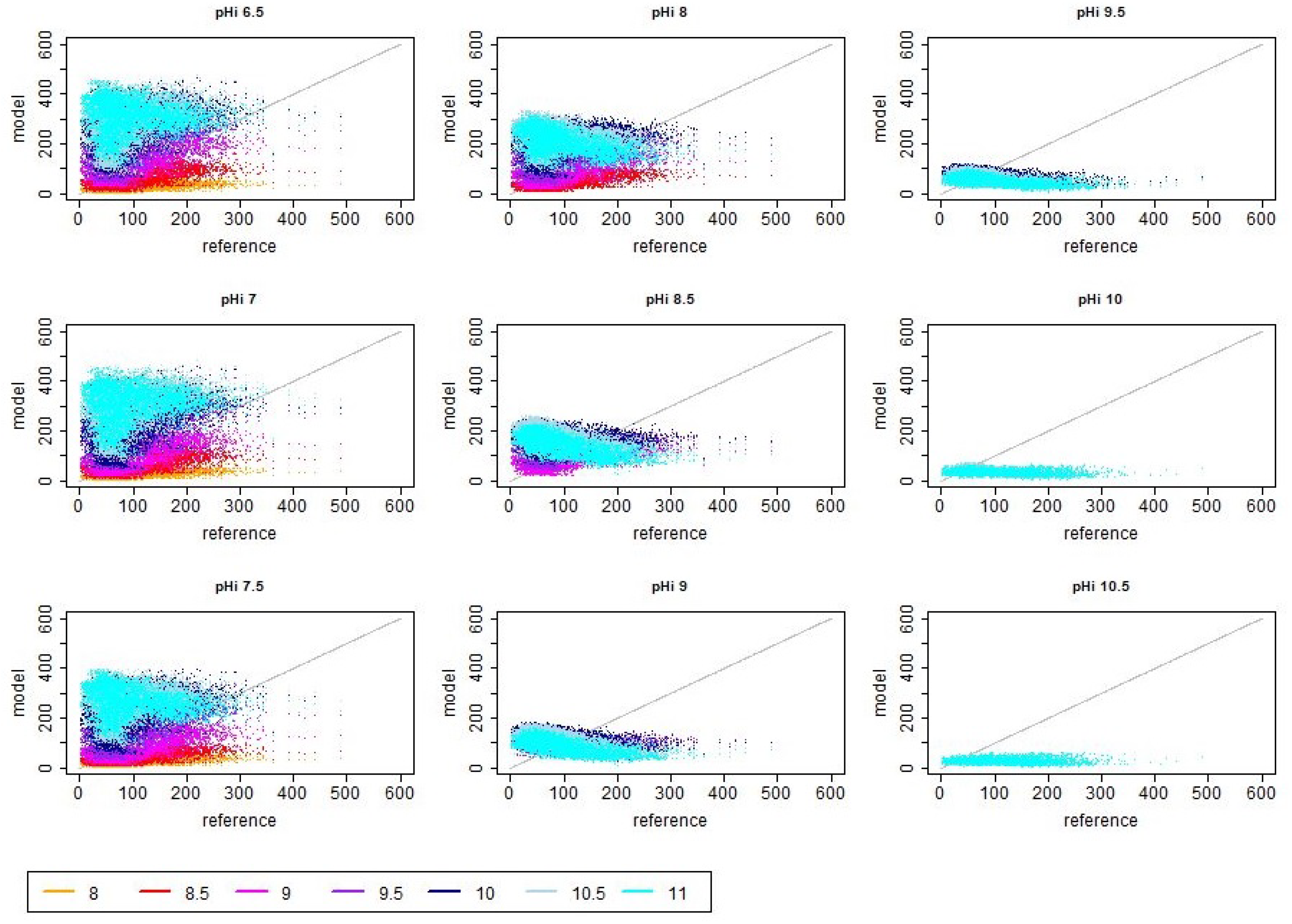
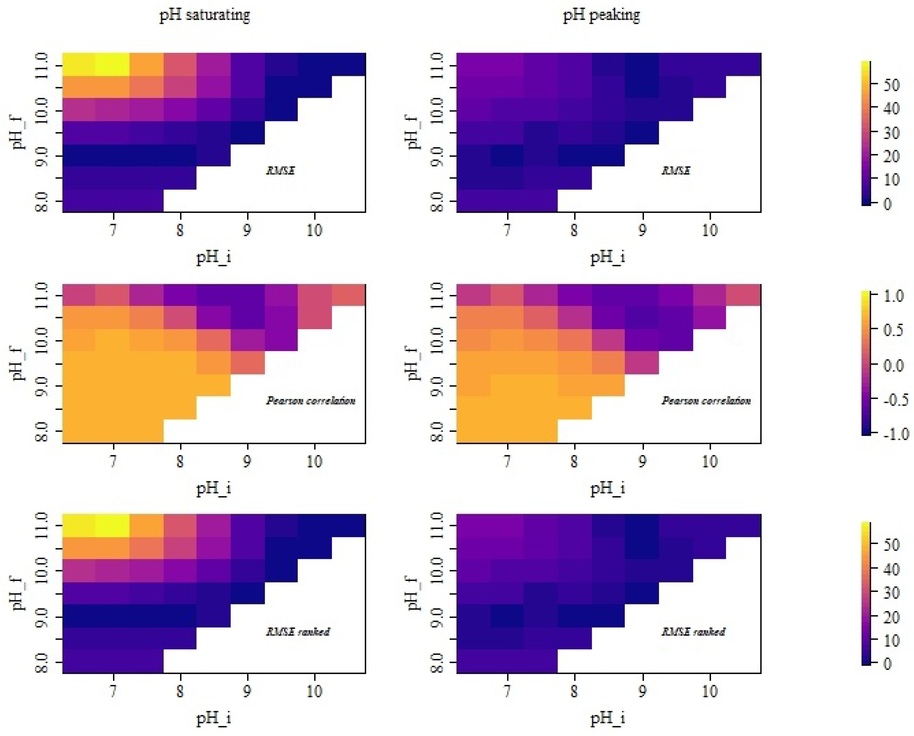
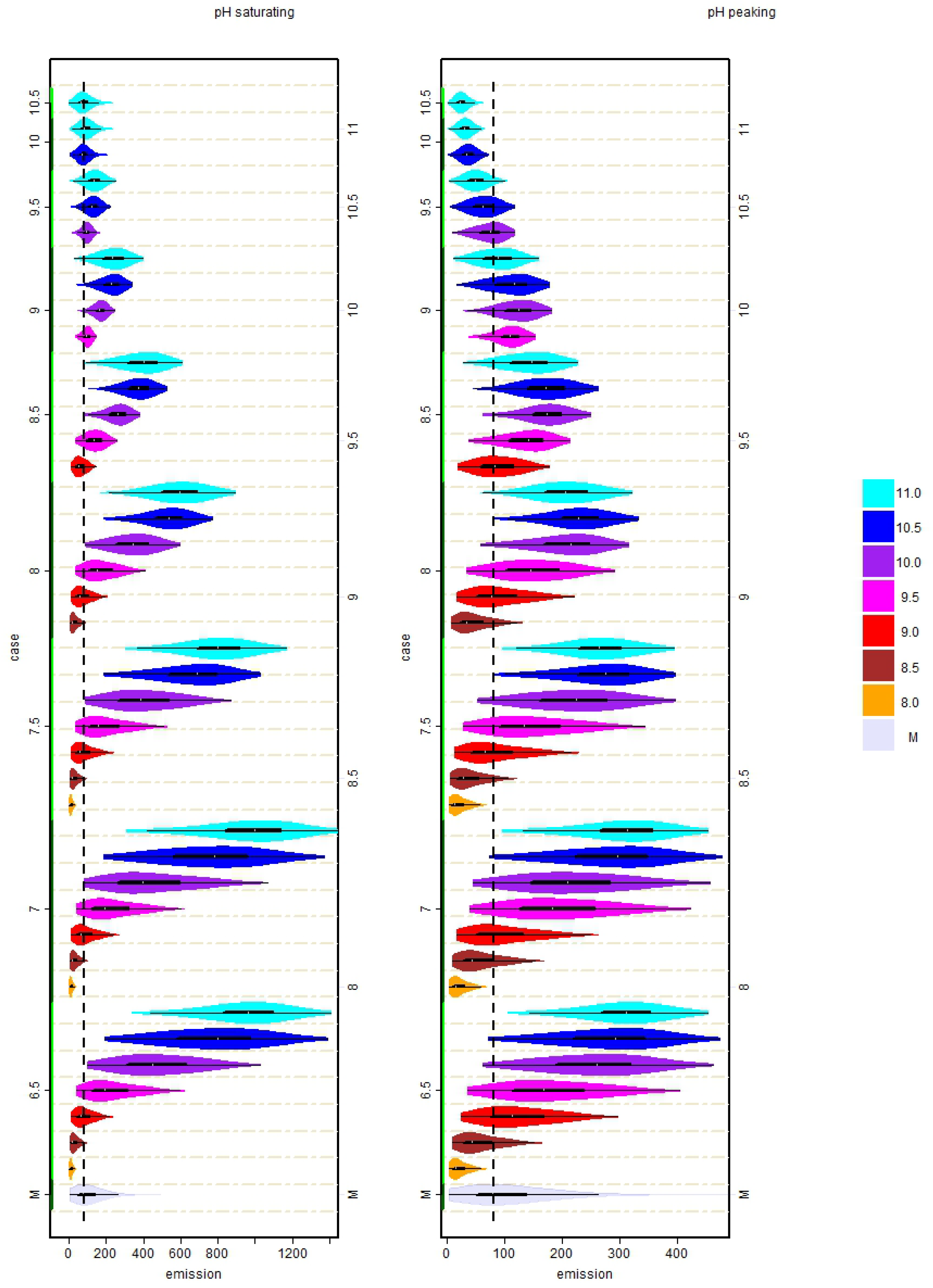
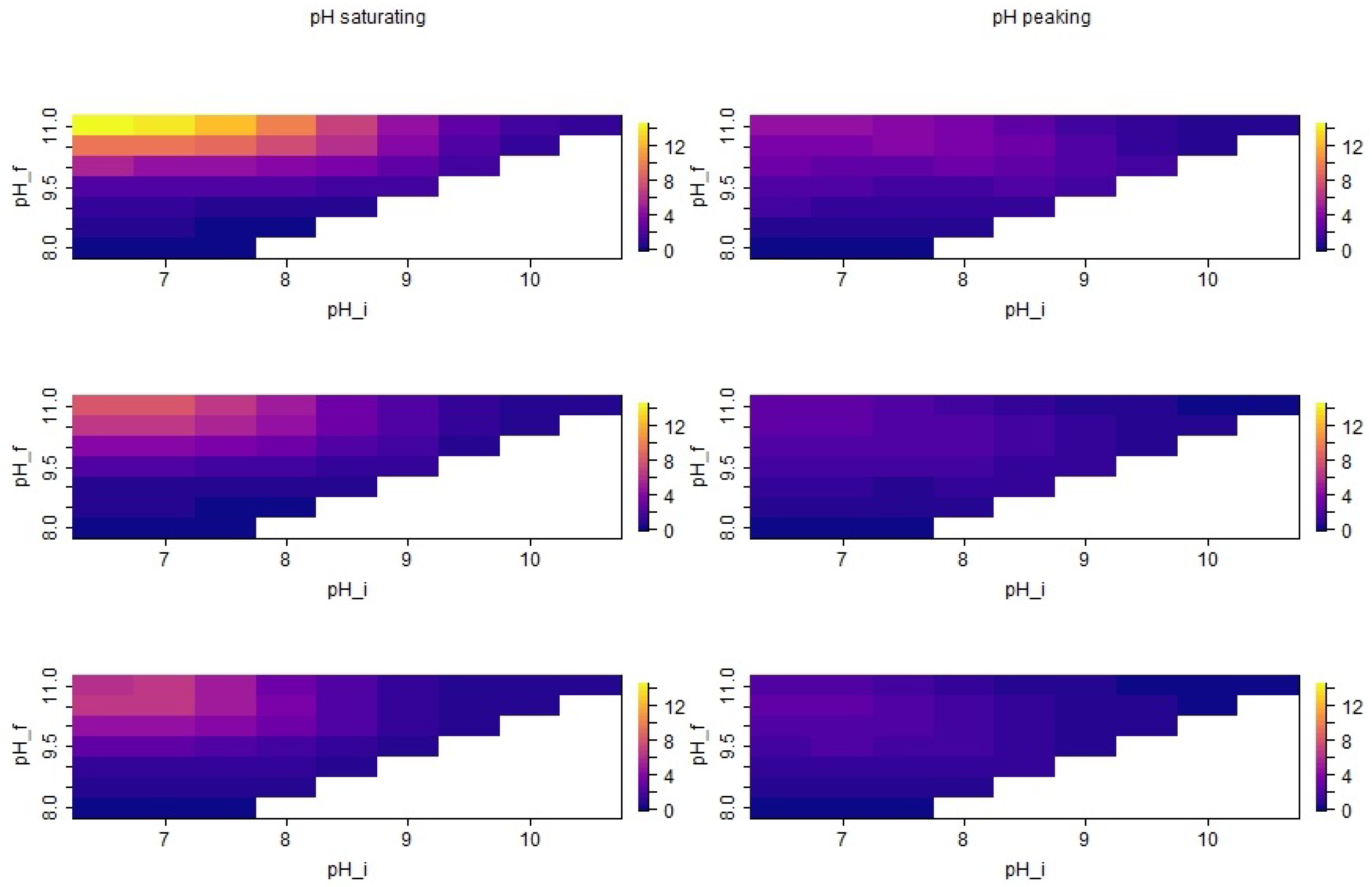
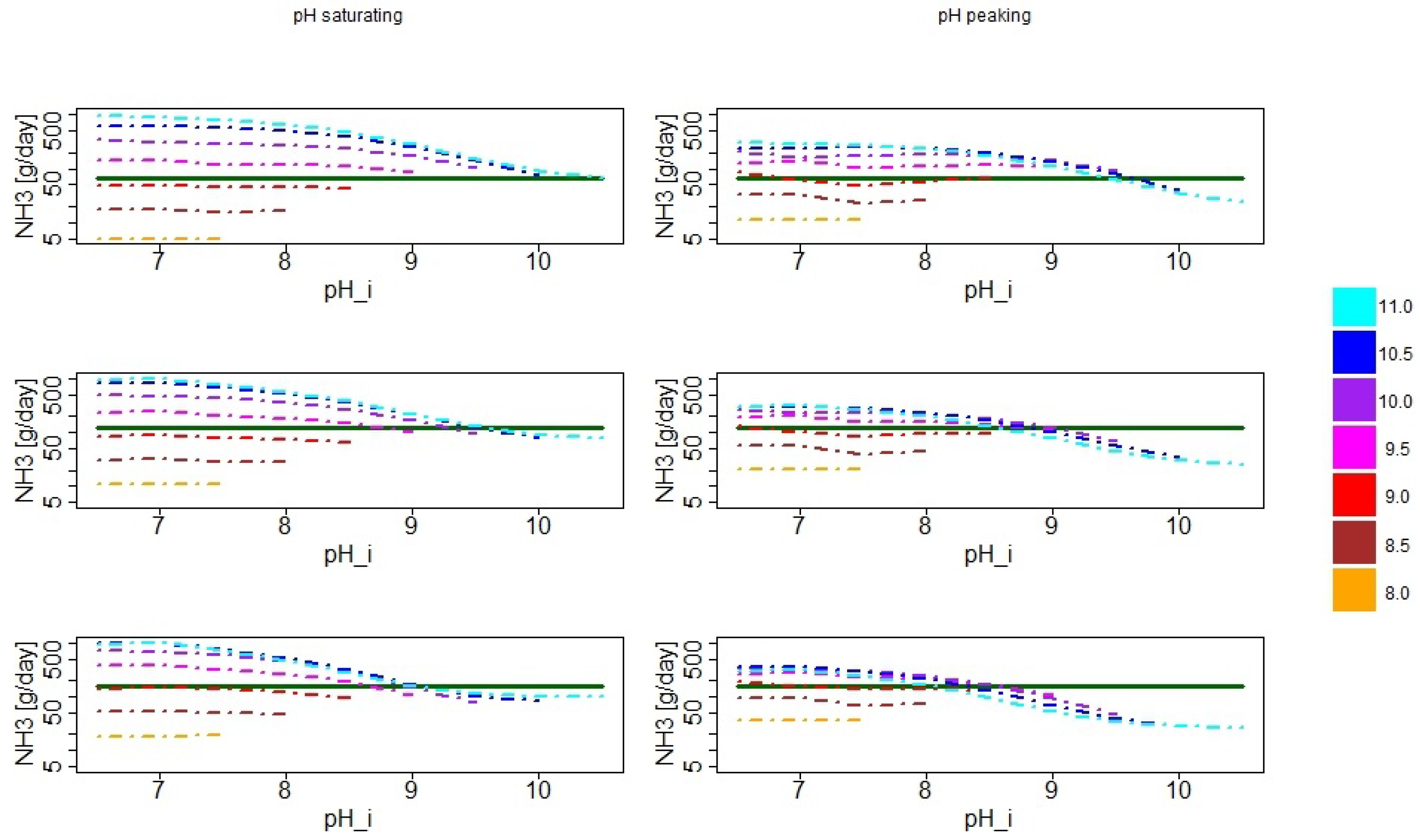
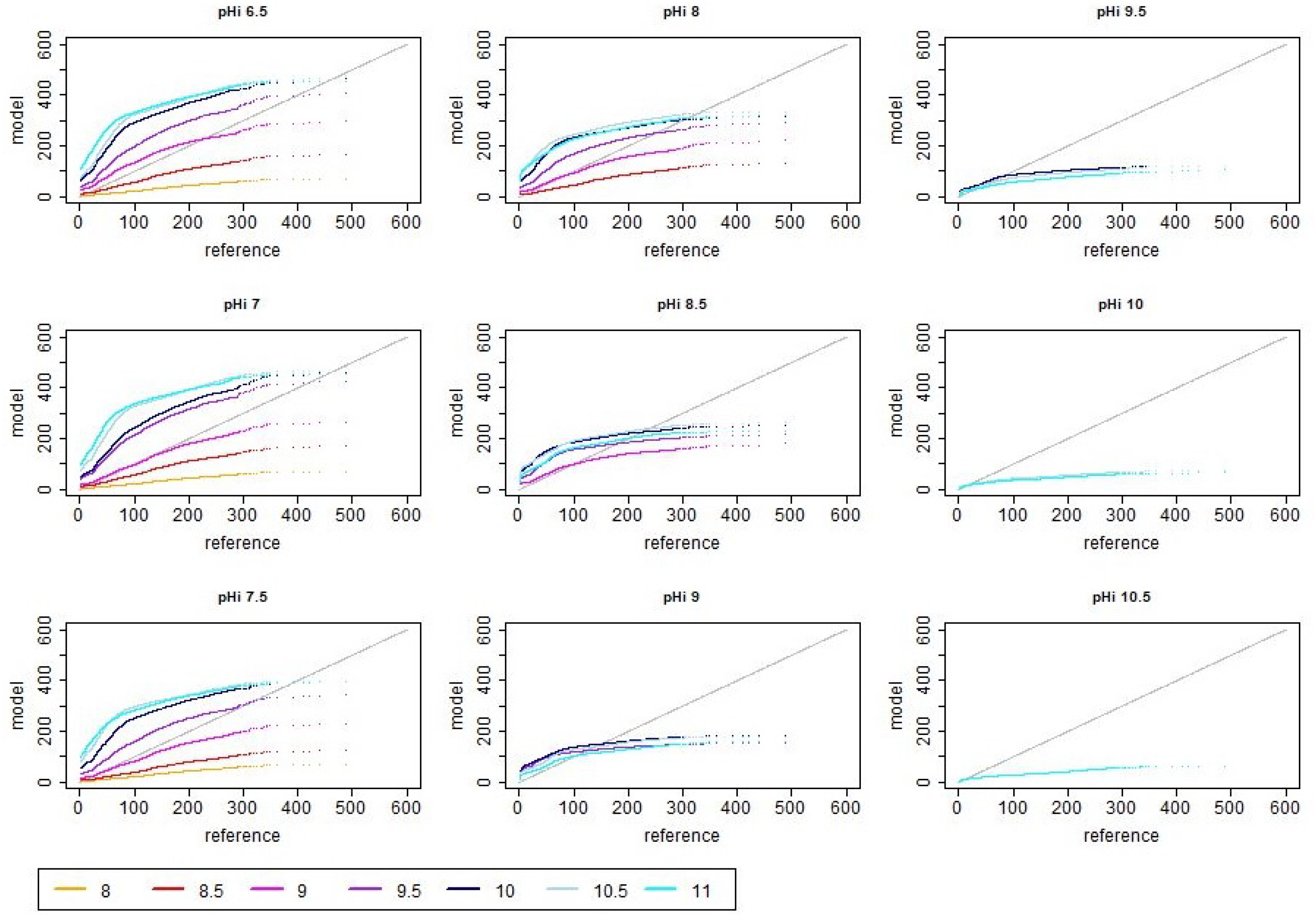
3.2. Distribution of Simulated Emission Values

In the saturating simulation case where the pH value increased over 24 h, the best match with the measured emission values in terms of variability, RMSE and correlation was found for $p{H}_i=7.0$ and $p{H}_i=7.5$ together with $p{H}_f=9.0$, as can be seen in Figure 3 and Figure 4 in the left panels. For the pair $p{H}_i=7.0$ and $p{H}_f=9.0$, this is not surprising as the parameter values are very close to the values for which the model was originally calibrated (i.e., $p{H}_i=6.8$ and $p{H}_f=9.2$, cf. [7]). In consequence, the distribution of the emission values in Figure 4 is very similar to that of the experimentally derived emission values. The comparison of all distributions of the simulated and experimentally derived emission values indicated that in the abovementioned simulation cases with $p{H}_i=7.0$ or $p{H}_i=7.5$ and $p{H}_f=9.0$, basically only the few very high emission peaks were not captured. At the same time, simulation cases with $p{H}_f>9$ typically yielded far less low emission values and resulted in more symmetric distributions, while the average emission value increased. In consequence, the temporal dynamics of the simulated emission values must not be expected to be similar to the dynamics of the experimentally derived emissions (which can be also seen in the scatter plots in the Appendix A Figure A1 and Figure A2). These systematic changes in the distribution of emission values are caused by the modified pH dynamics and may explain a part of the variability of on-farm emissions observed in practice even when the building design, herd composition and feed strategies are similar.

The scattering of the points in Figure A1 is centered around the line of identity for the case $p{H}_i=7.0$ and $p{H}_f=9.0$, as expected. However, the scatter plots also show that a comparable scattering of points can be obtained with the high values of $p{H}_i$ and $p{H}_f$ being closer together (e.g., $p{H}_i=8$ and $p{H}_i=8.5$ combined with $p{H}_f=9$ or $p{H}_f=9.5$), and it is also possible to obtain a similar scattering with very high $p{H}_i$ and $p{H}_f$ values (i.e., cases were $p{H}_i\ge 9.5$). However, in the mentioned cases with higher values of $p{H}_f$, the violin plots in Figure 4 also show that the shape of the distribution becomes rather different and that most of the lower emission values (normally typical for winter conditions) are missing.

Looking at the rank-order scatter plots (Figure A2), it can be further confirmed that the systematic bias was much higher when using the mentioned parameter combinations with the higher $p{H}_i$ values compared with the cases of $p{H}_i$ that ranged from $6.5$ to $8.0$ together with $p{H}_f=9.0$. Particularly, the combination of $p{H}_i=8.5$ and $p{H}_i=9$ with $p{H}_f=9.5$ led to a significant overestimation of the lower emission values, which was compensated by an underestimation of the higher emission values. This overestimation of the low emission values was decreasing for higher $p{H}_i$ values. This trend can be also seen in the top and bottom panels on the right of Figure 3 in the distribution of RMSE. The smallest errors were obtained when $p{H}_i<9$ and $p{H}_f=9$ or $p{H}_i\ge 9$ and $p{H}_f=p{H}_i+0.5$.

The RMSE of the original time series and of the ranks showed almost the same pattern, indicating that the temporal dependencies only barely affected the RMSE. This is also consistent with Figure A1 and Figure A2, where the former set shows high variability but generally similar trends compared with the latter.

The central panel of the left column of Figure 3 shows that the correlation between measurements and simulations follows a different trend than the RMSE with respect to $p{H}_i$ and $p{H}_f$. In general, the correlation became worse for higher asymptotic pH values (except for cases with very high $p{H}_i$), while for the RMSE, this was only the case for $p{H}_f\ge 9$. By far the best correlations were obtained for the lower $p{H}_i$ values together with $p{H}_f=p{H}_i+0.5$ or $p{H}_f=p{H}_i+1$. In contrast, some of the other parameter combinations that showed low RMSE had a vanishing correlation with the measurements or even showed anti-correlation.

If a decrease in pH after 10 h was considered, the overall emissions were increasing. In order to account for this effect, the assumed cleaning efficiency was adjusted in the simulations (i.e., cleaning was assumed to be more efficient, which is reflected in the model by a smaller value of the correction factor for the emission active surface $c_{eff}$). Afterwards the distribution of emission values, RMSE and correlations show in general similar trends as in the previous simulation cases with saturating pH. The main difference in the scatter plots is that in the cases with peaking pH, the spread is much lower, particularly for high $p{H}_f$ values (cf. Figure A1 vs. Figure A3). This reduced variability is also observed in the violin plots (cf. left vs. right panel in Figure 4). For most pH combinations (except for the very high initial pH values), the tendency for overestimation was lower in the cases with peaking pH (cf. also Appendix A Figure A3 and Figure A4). High correlation and low RMSE were particularly found for lower pH values with $p{H}_f$ being up to a value of 9 (see Figure 3 right panels). A particularly low RMSE was observed for the parameter combination $p{H}_i=7$ and $p{H}_f=9$ (for which $c_{eff}$ was tuned) but also for the combination $p{H}_i=8$ and $p{H}_f=9$, the combination $p{H}_i=8.5$ and $p{H}_f=9$ and the combination $p{H}_i=9$ and $p{H}_f\ge 9.5$. The mentioned combinations with $p{H}_i=9$, however, were associated with an anti-correlation between the simulated and measured emissions. The best correlations (i.e., values of about 0.64) were obtained for the simulation cases with $p{H}_f=8$ and all considered $p{H}_i$ as well as with $p{H}_i=7$, $p{H}_f=8.5$ and $p{H}_i=7.5$, $p{H}_f=8.5$. The range of observed correlation values for the simulations with non-monotonic pH dynamics was very similar to the set of simulations with saturating pH. At the same time, the maximal observed RMSE was much lower for the non-monotonic pH dynamics (cf. Figure 3).

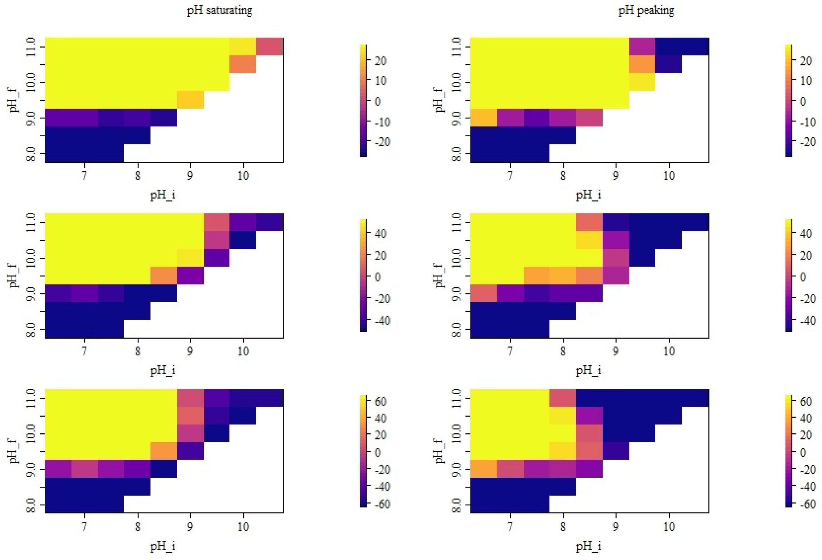
3.3. Seasonal Effects of pH Dynamics

As shown in Figure 5, the relative deviation of the simulation from the measurements became typically larger when the deviation between $p{H}_i$ and $p{H}_f$ was increasing. Moreover, the deviation from the measurements was largest when low values of $p{H}_i$ were combined with high values of $p{H}_f$. Both effects were less pronounced when the pH was decreasing after 10 h compared with a saturating pH assumption. Overall, the largest relative deviations were observed in winter. In Figure 6, the absolute deviations between the simulation and measurement were plotted for all pH combinations and showed a relative deviation of less than ±40% from the measurements. It can be seen that considerable overestimation and underestimation can be found for some pH parameter combinations and seasons.

Only with $p{H}_f=9$ did almost all considered combinations result in absolute deviations within the considered range of uncertainty. With $p{H}_f=9$, assuming the saturating pH resulted in an underestimation for all seasons and initial pH values (cf. Figure 6 left column). The level of underestimation was strongest in the transition season and showed an increasing trend for higher initial pH values. When a decrease in the pH after 10 h was considered, the trends over the seasons for $p{H}_f=9$ were similar to the previously described situation (cf. Figure 6 right column): Typically, higher initial pH resulted in lower seasonal emission values, and underestimation was most pronounced in the transition season.

In Figure 7, the actual simulated seasonal emission values for the different pH settings are shown together with the associated reference values. Here, it can be seen even better that around initial pH values around 8.5 and $p{H}_f=p{H}_i+0.5$, the model started to flip from underestimation to overestimation. In the case of the saturating scenario, this flipping occurred for similar initial pH values in all seasons. In the peaking scenario, it already occurred between 8.0 and 8.5 in summer, between 8.5 and 9.0 in transition and only around 9.5 in winter.

For very high $p{H}_i$ and $p{H}_f$, an underestimation in summer and transition season was observed in the saturating and, particularly, in the peaking pH scenarios (see also

Table 3. Simulated average emission values (winter/transition/summer) in g day${}^{-1}$ for the saturating $pH$ setting. Rows refer to the initial pH $p{H}_i$ and columns refer to the asymptotic pH $p{H}_f$ that was used in the different simulation cases. The associated reference values were 66 g day${}^{-1}$/125 g day${}^{-1}$/157 g day${}^{-1}$ for the three seasons.

$\mathit{pH}$	8.0	8.5	9.0	9.5	10.0	10.5	11.0
6.5	5/11/18	17/31/52	49/85/135	143/240/375	349/512/708	632/826/1029	939/970/949
7.0	5/11/18	17/32/53	49/91/151	144/242/376	299/470/693	616/811/1015	923/1004/1035
7.5	5/11/19	15/29/50	44/81/135	120/204/320	295/434/601	577/700/796	810/809/746
8.0	-/-/-	16/29/48	44/76/121	118/183/268	276/367/456	505/548/544	653/589/477
8.5	-/-/-	-/-/-	42/66/95	107/147/189	235/272/288	393/376/317	464/379/275
9.0	-/-/-	-/-/-	-/-/-	86/100/106	171/171/151	259/221/168	283/220/160
9.5	-/-/-	-/-/-	-/-/-	-/-/-	102/93/79	143/121/102	154/129/114
10.0	-/-/-	-/-/-	-/-/-	-/-/-	-/-/-	75/77/83	90/92/101
10.5	-/-/-	-/-/-	-/-/-	-/-/-	-/-/-	-/-/-	68/81/98

and

Table 4. Simulated average emission values (winter/transition/summer) in g day${}^{-1}$ for the peaking $pH$ setting. Rows refer to the initial pH $p{H}_i$ and columns to the asymptotic pH $p{H}_f$ that was used in the different simulation cases. The associated reference values were 66 g day${}^{-1}$/125 g day${}^{-1}$/157 g day${}^{-1}$ for the three seasons.

$\mathit{pH}$	8.0	8.5	9.0	9.5	10.0	10.5	11.0
6.5	11/21/37	33/58/95	85/132/194	128/191/271	208/269/337	241/296/353	306/310/305
7.0	11/21/37	33/59/96	59/100/158	141/206/287	162/231/314	244/299/356	293/313/325
7.5	11/21/36	22/40/67	49/85/136	102/156/227	177/233/295	245/276/297	271/265/246
8.0	-/-/-	26/46/75	58/93/141	113/159/212	183/216/243	230/231/216	231/203/163
8.5	-/-/-	-/-/-	65/94/128	118/145/168	171/176/166	193/169/131	173/136/94
9.0	-/-/-	-/-/-	-/-/-	108/112/105	138/121/92	136/105/69	110/80/52
9.5	-/-/-	-/-/-	-/-/-	-/-/-	90/69/47	79/57/39	61/45/34
10.5	-/-/-	-/-/-	-/-/-	-/-/-	-/-/-	41/34/29	34/30/29
10.5	-/-/-	-/-/-	-/-/-	-/-/-	-/-/-	-/-/-	24/25/27

). In the peaking scenario, the observed underestimation was already nearly one order of magnitude. In the saturating scenario, this underestimation in summer and transition came with a small overestimation in winter season, while in the peaking pH scenario, a considerable underestimation was also observed in winter.

4. Discussion

4.1. Conclusions on Actual pH Dynamics

The measured pH values in the case study barn ranged between 6.8 and 8.6. This fits well with the estimated pH dynamics when selecting $p{H}_i=7$ and $p{H}_f=9$. Those values were among the parameter combinations with the best matches with the observed long-term NH${}_3$ emission dynamics. In this context, it has to be noted that the match in terms of absolute emission level is of little significance, as it strongly depends on the value of the theoretical cleaning efficiency, which was used as a tuning parameter in the simulation. Thus, a good match in our study mainly refers to high correlations and a good representation of the seasonal differences in the emission patterns, as those features are strongly affected by the assumed pH dynamics.

In both simulation settings, i.e., with saturating and with peaking pH dynamics, the assumed functional relations with the $p{H}_i=7$ and $p{H}_f=9$ predicted pH values was around $8.5$ for puddles with an age of around two hours (cf. Figure 2). This age of two hours is the likely maximum age of most of the urine volume in the barn as the time span is close to the scrapping frequency. Hence, the parameter combination mentioned above probably reflects the actual pH range well. The question of when urine puddle pH starts to decrease, however, remains open, as both simulations settings (i.e., assuming pH only decreased after more than 24 h versus assuming that pH decreased after 10 h) did not differ considerably in terms of the quality of the prediction of the long-term ammonia emission dynamics with the parameter combination $p{H}_i=7$ and $p{H}_f=9$. Moreover, based on the literature, it is likely that the turning point in the pH dynamics will vary from barn to barn, from season to season and maybe even from puddle to puddle [25].

In contrast to the measurements, a theoretical initial pH value of 8.3 was estimated based on the available information on feed chemical composition for the herd under study; this value is very close to the highest measured pH in the urine puddles. Starting with a pH value of 8.5 (which is closest to this theoretical value among the considered initial values) resulted in an acceptable RMSE and a correlation with the measurements if $p{H}_f=9$ was selected. But the seasonal variation of emission dynamics was not well reproduced in that case, implying that this theoretical value may not reflect the average initial pH value well.

However, it must be noted that a constant initial urine pH value was considered in our simulations, whereas the actual initial pH may vary during the day in dependence of the temporal distance between feeding and urination as well as over the course of the year. Snoek et al. found in time series measurements of a 4 h duration that urine puddle pH increased more slowly in summer than in winter and that pH curves were more dynamic in winter [25]. They assumed that the differences in the dynamical behavior might be the result of different feeding strategies or feed composition in summer and winter. On the other hand, Kadzere et al. mentioned a relation between heat stress and raising urine pH that was reported in the literature, which would imply that diurnal variation in urine pH has to be expected, particularly in summer season [29]. Moreover, Dancher et al. reported physiological diurnal fluctuations in the fecal and urinary pH of Danish Holstein cows, which they associated with variations in feed intake, transit time, fermentation patterns, absorption of metabolites and pH in the rumen and hindgut over the course of the day [30]. In consequence, it might be that the mentioned theoretical initial urine pH value for our considered herd reflected a maximum rather than a daily average urine pH. However, in their study, Dancher et al. did not mention the amplitude of the diurnal fluctuations of urine pH. The question of how and to which extent the average urine pH value is modulated in response to the feeding strategy (e.g., the time of feeding and the duration of feed availability) remains open. Also, the effect of heat stress on urine pH is only described qualitatively in the literature. In another study, Roche et al. also showed small diurnal variations in the urine pH of non-lactating Holstein-Friesian cows with access to hay for about 10 h per day, but they concluded that there is no significant diurnal variation in the urine pH [31].

This highlights that further studies on the diurnal and seasonal urine pH variations and their influencing factors are crucial for obtaining a more representative urine pH model to drive our ammonia emission model without extensive on-farm urine puddle sampling.

4.2. Impact of pH Dynamics on Total Ammonia Emission

In the simulations, it was observed that for the parameter settings with high asymptotic pH and low initial pH, summer emissions were considerably reduced compared with the “real-barn” dynamics while winter emissions were slightly reduced. This even led to counter-intuitive seasonal emission patterns for some parameter combinations (cf. also the results reported in [21]).

This effect might be explained by the presence of different fractions of NH${}_3$ and NH${}_4^{+}$ in the urine puddles. Each puddle is an aqueous solution where NH${}_3$ and NH${}_4^{+}$ are in a chemical equilibrium, but only NH${}_3$ will volatilize from the solution to the surrounding environment [24,32]. In our simulation model, the ammonia fraction was approximated following the equation suggested by Elzing and Monteny 1997 (see Equation (7)) for manure and urine puddles in cattle houses [15]. This definition of the fraction was adapted from an earlier study on chicken manure by Hashimoto and Kudington 1971 [33].

$$f=\frac{100}{1+\frac{{10}^{-pH}}{0.81 \times {10}^{-10} \times {1.07}^{(T-20)}}}$$

(7)

Here, T is the temperature of the puddle in ${}^{\circ }$C, $pH$ is the pH value of the puddle and f is the ammonia fraction in %. In this equation, the actual ammonia fraction at a particular time point depends on the temperature and pH of the urine puddle at this time point. Alkali regimes and high temperatures shift the equilibrium towards NH${}_3$, while acid regimes and low temperatures favor NH${}_4^{+}$. Following Equation (7), for a urine puddle temperature that is close to body temperature, there would be a 50:50 ratio of NH${}_3$:NH${}_4^{+}$ for pH values around 9.5, while at pH = 11, almost all of the ammoniacal nitrogen would be NH${}_3$. At a temperature of 20 ${}^{\circ }$C, the 50:50 ratio would be achieved for a pH slightly above 10 and, for around the freezing point of water, a pH of around 10.5 would result in the 50:50 ratio of NH${}_3$:NH${}_4^{+}$.

As urine puddles tend to cool down and alkalize during the emission process, a shift in the NH${}_3$:NH${}_4^{+}$ ratio must be expected. Based on Equation (7), in the beginning of the emission process (i.e., when temperature is high and the pH is low), the ammonia fraction would be lower the higher that the assumed maximum pH value is. Later, when the temperature of the puddle is considerably lower but the pH is higher, the opposite trend can be true (i.e., a higher maximum pH would be associated with a higher ammonia fraction). However, at this later time point, the total amount of ammoniacal nitrogen will be lower due to the conversion of urea and the cleaning of the floor. Thus, the impact on the overall emission is not straightforward.

When pH${}_i$ is already high in the beginning, there will be a large portion of NH${}_3$ independent of the temperature. In consequence, the emission pattern must be expected to be rather uniform throughout the different temperature regimes, i.e., throughout the seasons. This is well in line with the pattern that we observed for pH${}_i\ge 10$. Here, we found almost the same average emission value in summer and in winter in the simulation.

When considering a simplified simulation case with a hypothetical air temperature of 10 ${}^{\circ }$C and the a selection of high and low $p{H}_i$ and $p{H}_f$ values, the emission behavior can be linked with the change in the ammonia fraction over time (cf. Figure 8). In the settings with high $p{H}_i$ values, it turned out that the total ammoniacal nitrogen concentration was very high in the beginning but already dropped during the first hour of integration. Then, it increased again slightly (the lower the ambient temperature was). Finally, in the long run, the total ammoniacal nitrogen concentration decreased very slowly. As a consequence, although the portion of ammonia was very high at those high pH values, the total ammonia emission was low in this setting.

In contrast, when the maximum pH was high but the initial pH value was much lower than 10, the drop in total ammoniacal nitrogen concentration occurred later and was less sharp in the simulation. In those cases, there was no considerable intermittent increase in the total ammoniacal nitrogen concentration. Considering the whole 24 h period of integration, the total ammonia emission was higher for the lower initial pH values than in the case of the very high pH${}_i$.

In practice, typically much lower maximum pH values are reported, e.g., a range of 5.5 to 8.3 [17], 7 to 8.6 [34] or 8.1 to 9.4 [25]. In these pH regimes, the behavior outlined above will not occur as the total ammoniacal nitrogen concentration increases and decreases very slowly in the simulations. Here, lower initial pH values in the simulations were associated with lower emissions. This is well in line with the observations in practice, where acidification of slurry is used as an ammonia mitigation measure (e.g., [35,36,37]).

In contrast, very low initial combined with very high asymptotic pH values have not been reported in the literature about cattle urine puddles and might thus be only a hypothetical case. However, a chemical reaction with non-standard flooring material could potentially also result in higher pH levels. Moreover, almost instantaneous treatment of the fresh puddle of urine is conceivable. Although artificially increasing the pH value in urine storage is not common in the agricultural context, it is used in other fields of application. In the context of waste water treatment, for example, Larsen et al. 2021 highlighted that the alkaline stabilization of urea with urine pH values of about 10 using wood ash can be considered a valid alternative to acidic stabilization [38]. Moreover, in the context of slurry storage and utilization, the process of alkalization is also reported as a method to reduce emissions [39,40]. In contrast to the observed behavior in our simulation, the main line of argumentation in the literature is, however, that shifting the equilibrium towards NH${}_3$ by increasing the pH value results in high ammonia concentrations, which can be captured to produce ammonium-based mineral fertilizers. Alkalization at a very early stage is recommended to minimize the consumption of bases due to the complex interaction of different pH buffering systems in the slurry. Such a scenario of pH change could be associated with the simulations cases where we start with a rather low initial pH and have a very sharp increase towards high pH values, i.e., low $p{H}_i$ and high $p{H}_f$. However, the mentioned buffering effects have so far not been mapped in our pH model.

5. Conclusions

We systematically reviewed the effect of 42 settings of pH dynamics on the projection of the long-term ammonia emission pattern of a naturally ventilated dairy cattle building with solid floors. We showed that the non-linear interaction of the puddle pH and temperature caused specific emission patterns, where the degree of influence of the two parameters changed over the course of the emission process. In consequence, even with the same initial or average pH value, the same initial concentration of urea and total ammoniacal nitrogen may result in different emission patterns, yielding partly considerably different annually averaged emission values. Thus, potential barn management or design settings (e.g., flooring material or cleaning systems) that may affect the temporal evolution of the pH value of urine puddles should be considered more in terms of their potential impacts on the emission of $N{H}_3$ in the future. Particularly due to the effects of evaporation and cleaning, the total amount of nitrogen that is released from the urine puddle by means of $N{H}_3$ emission can vary; this is the case even on longer time scales despite the initial nitrogen content of the puddle being the same (i.e., it is not that “everything” comes out anyway). The key findings were derived from the simulation setup as follows.

Low initial pH values together with high asymptotic pH values were associated with the largest emissions. Considering the same asymptotic pH value, the emission was lower the higher that the chosen initial pH value was. This indicates that acidification of urine or slurry as an emission mitigation measure requires that the pH level is kept low over a longer period of time, as a fast pH increase over time may considerably amplify the total emissions. Attempts to control the total ammonia emission by modifying the pH should focus on limiting the highest pH values but also avoid steep gradients in pH change over time.

Assuming peak pH dynamics, the emission values were significantly lower. This highlights the specific relevance of pH in the late phase of the emission process when the puddle temperature was fairly low and the emission active surface area was greatly reduced. This role of the late phase of the emission process further caused specific seasonal effects. In natural pH settings (i.e., low to intermediate initial pH and intermediate asymptotic pH), the winter emissions were considerably lower than the summer emissions. In contrast, artificial pH settings with high pH values led to considerably lower emissions in the summer, reducing the total annual emission value. Whether such moderation of the pH dynamics would be feasible in practical applications, however, has to be further investigated in future studies. Those future studies should also investigate the range of naturally occurring pH dynamics in urine puddles in cattle barns, which might be influenced by many factors, e.g., by the flooring material, entry of litter or feed leftovers, the cleaning systems (e.g., use of water), or the cooling system (e.g., use of misters).

In addition, the coupled semi-mechanistic model needs to be further refined (e.g., to capture better urination and cleaning patterns and incorporate the dynamic, bidirectional interaction between the puddle pH and the emission source strength itself). The latter is so far only implemented as a unidirectional relation (i.e., pH influences the emission source strength). Thus, in future studies, it needs to be evaluated to which degree the observed pH dynamics and the resulting emission pattern persist when the change in the pH would be dynamically coupled to the actual instantaneous emission source strength, as some feedback loops may dampen the effects noticed.

References

1. Huang, T.; Gao, B.; Hu, X.K.; Lu, X.; Well, R.; Christie, P.; Bakken, L.R.; Ju, X.T. Ammonia-oxidation as an engine to generate nitrous oxide in an intensively managed calcareous Fluvo-aquic soil. Sci. Rep. 2014, 4, 3950. [Google Scholar] [CrossRef] [PubMed]
2. Behera, S.N.; Sharma, M. Degradation of SO2, NO2 and NH3 leading to formation of secondary inorganic aerosols: An environmental chamber study. Atmos. Environ. 2011, 45, 4015–4024. [Google Scholar] [CrossRef]
3. OECD. Trends and Drivers of Agri-Environmental Performance in OECD Countries; OECD Publishing: Paris, France, 2019; p. 105. [Google Scholar] [CrossRef]
4. European Environment Agency (EEA). European Union Emission Inventory Report 1990–2017; European Environment Agency (EEA): Copenhagen, Denmark, 2019; Volume 8.
5. Dai, X.; Karring, H. A determination and comparison of urease activity in feces and fresh manure from pig and cattle in relation to ammonia production and pH changes. PLoS ONE 2014, 9, e110402. [Google Scholar] [CrossRef] [PubMed]
6. Vaddella, V.; Ndegwa, P.; Jiang, A. An empirical model of ammonium ion dissociation in liquid dairy manure. Trans. ASABE 2011, 54, 1119–1126. [Google Scholar] [CrossRef]
7. Hempel, S.; Ouatahar, L.; Janke, D.; Doumbia, E.M.; Willink, D.; Amon, B.; Bannink, A.; Amon, T. Ammonia emission prediction for dairy cattle housing from reaction kinetic modeling to the barn scale. Comput. Electron. Agric. 2022, 199, 107168. [Google Scholar] [CrossRef]
8. Mielcarek-Bocheńska, P.; Rzeźnik, W. Odors and ammonia emission from a mechanically ventilated fattening piggery on deep litter in Poland. Arch. Environ. Prot. 2022, 48, 86–94. [Google Scholar]
9. Snell, H.; Seipelt, F.; Van den Weghe, H. Ventilation rates and gaseous emissions from naturally ventilated dairy houses. Biosyst. Eng. 2003, 86, 67–73. [Google Scholar] [CrossRef]
10. Janke, D.; Willink, D.; Ammon, C.; Hempel, S.; Schrade, S.; Demeyer, P.; Hartung, E.; Amon, B.; Ogink, N.; Amon, T. Calculation of ventilation rates and ammonia emissions: Comparison of sampling strategies for a naturally ventilated dairy barn. Biosyst. Eng. 2020, 198, 15–30. [Google Scholar] [CrossRef]
11. Bannink, A.; Spek, W.J.; Dijkstra, J.; Šebek, L.B. A Tier 3 method for enteric methane in dairy cows applied for fecal N digestibility in the ammonia inventory. Front. Sustain. Food Syst. 2018, 2, 66. [Google Scholar] [CrossRef]
12. Bjerg, B.; Cascone, G.; Lee, I.B.; Bartzanas, T.; Norton, T.; Hong, S.W.; Seo, I.H.; Banhazi, T.; Liberati, P.; Marucci, A.; et al. Modelling of ammonia emissions from naturally ventilated livestock buildings. Part 3: CFD modelling. Biosyst. Eng. 2013, 116, 259–275. [Google Scholar] [CrossRef]
13. Saha, C.K.; Zhang, G.; Ni, J.Q. Airflow and concentration characterisation and ammonia mass transfer modelling in wind tunnel studies. Biosyst. Eng. 2010, 107, 328–340. [Google Scholar] [CrossRef]
14. Rong, L.; Nielsen, P.V.; Zhang, G. Effects of airflow and liquid temperature on ammonia mass transfer above an emission surface: Experimental study on emission rate. Bioresour. Technol. 2009, 100, 4654–4661. [Google Scholar] [CrossRef] [PubMed]
15. Elzing, A.; Monteny, G. Modeling and experimental determination of ammonia emissions rates from a scale model dairy-cow house. Trans. ASAE 1997, 40, 721–726. [Google Scholar] [CrossRef]
16. Snoek, D.J.; Stigter, J.D.; Ogink, N.W.; Koerkamp, P.W.G. Sensitivity analysis of mechanistic models for estimating ammonia emission from dairy cow urine puddles. Biosyst. Eng. 2014, 121, 12–24. [Google Scholar] [CrossRef]
17. Melendez, P.; Bartolome, J.; Roeschmann, C.; Soto, B.; Arevalo, A.; Möller, J.; Coarsey, M. The association of prepartum urine pH, plasma total calcium concentration at calving and postpartum diseases in Holstein dairy cattle. Animal 2021, 15, 100148. [Google Scholar] [CrossRef] [PubMed]
18. Snoek, D.J.; Stigter, J.D.; Kupers, G.C.; Koerkamp, P.W.G.; Ogink, N.W. Assessing fresh urine puddle chemistry in commercial dairy cow houses. Biosyst. Eng. 2017, 159, 143–153. [Google Scholar] [CrossRef]
19. Kume, S.; Sato, T.; Murai, I.; Kitagawa, M.; Nonaka, K.; Oshita, T. Relationships between urine pH and electrolyte status in cows fed forages. Anim. Sci. J. 2011, 82, 456–460. [Google Scholar] [CrossRef] [PubMed]
20. Gulhane, H.; Nakanekar, A.; Mahakal, N.; Bhople, S.; Salunke, A. Gomutra (cow urine): A multidimensional drug review article. Int. J. Res. Ayurveda Pharm. 2017, 8, 1–6. [Google Scholar] [CrossRef]
21. Hempel, S.; Ouatahar, L.; Janke, D.; Amon, T. A nested semi-mechanistic model to predict the temporal dynamics of ammonia emissions from a solid floor naturally ventilated dairy cattle building—Parameter estimation and associated uncertainties. In Proceedings of the International Conference on Agricultural Engineering AgEng-LAND.TECHNIK 2022, Berlin, Germany, 22–23 November 2022; VDI Wissensforum GmbH: Düsseldorf, Germany, 2022; Volume 2406, pp. 197–202, ISBN 978-3-18092406-9. [Google Scholar]
22. Tabase, R.K. Mimicking indoor climate dynamics and ammonia emissions in a pig housing compartment using artificial pigs and an automatic urea spraying installation. Agric. Eng. Int. Cigr J. 2019, 21, 40–50. [Google Scholar]
23. Qu, Q.; Groot, J.C.; Zhang, K.; Schulte, R.P. Effects of housing system, measurement methods and environmental factors on estimating ammonia and methane emission rates in dairy barns: A meta-analysis. Biosyst. Eng. 2021, 205, 64–75. [Google Scholar] [CrossRef]
24. Cortus, E.; Lemay, S.; Barber, E.; Hill, G.; Godbout, S. A dynamic model of ammonia emission from urine puddles. Biosyst. Eng. 2008, 99, 390–402. [Google Scholar] [CrossRef]
25. Snoek, D.J.; Ogink, N.W.; Stigter, J.D.; Agricola, S.; Van de Weijer, T.M.; Koerkamp, P.W.G. Dynamic behavior of PH in fresh urine puddles of dairy cows. Trans. ASABE 2016, 59, 1403–1411. [Google Scholar]
26. Sommer, S.; Sherlock, R. pH and buffer component dynamics in the surface layers of animal slurries. J. Agric. Sci. 1996, 127, 109–116. [Google Scholar] [CrossRef]
27. Doumbia, E.M.; Janke, D.; Yi, Q.; Amon, T.; Kriegel, M.; Hempel, S. CFD modelling of an animal occupied zone using an anisotropic porous medium model with velocity depended resistance parameters. Comput. Electron. Agric. 2021, 181, 105950. [Google Scholar] [CrossRef]
28. Piccione, G.; Caola, G.; Refinetti, R. Daily and estrous rhythmicity of body temperature in domestic cattle. BMC Physiol. 2003, 3, 1–8. [Google Scholar] [CrossRef] [PubMed]
29. Kadzere, C.T.; Murphy, M.; Silanikove, N.; Maltz, E. Heat stress in lactating dairy cows: A review. Livest. Prod. Sci. 2002, 77, 59–91. [Google Scholar] [CrossRef]
30. Danscher, A.M.; Li, S.; Andersen, P.H.; Khafipour, E.; Kristensen, N.B.; Plaizier, J.C. Indicators of induced subacute ruminal acidosis (SARA) in Danish Holstein cows. Acta Vet. Scand. 2015, 57, 39. [Google Scholar] [CrossRef]
31. Roche, J.R.; Dalley, D.E.; O’Mara, F.P. Effect of a metabolically created systemic acidosis on calcium homeostasis and the diurnal variation in urine pH in the non-lactating pregnant dairy cow. J. Dairy Res. 2007, 74, 34–39. [Google Scholar] [CrossRef]
32. Ni, J. Mechanistic models of ammonia release from liquid manure: A review. J. Agric. Eng. Res. 1999, 72, 1–17. [Google Scholar] [CrossRef]
33. Hashimoto, A.; Ludington, D. Ammonia desorption from concentrated chicken manure slurries. In Livestock Waste Management and Pollution Abatement; ASABE: St. Joseph, MI, USA, 1971; pp. 117–121. [Google Scholar]
34. Afsahi, A.; Ahmadi-Hamedani, M.; Khodadi, M. Comparative evaluation of urinary dipstick and pH-meter for cattle urine pH measurement. Heliyon 2020, 6, e03316. [Google Scholar] [CrossRef]
35. Petersen, S.O.; Andersen, A.J.; Eriksen, J. Effects of cattle slurry acidification on ammonia and methane evolution during storage. J. Environ. Qual. 2012, 41, 88–94. [Google Scholar] [CrossRef] [PubMed]
36. Fangueiro, D.; Hjorth, M.; Gioelli, F. Acidification of animal slurry–a review. J. Environ. Manag. 2015, 149, 46–56. [Google Scholar] [CrossRef] [PubMed]
37. Misselbrook, T.; Hunt, J.; Perazzolo, F.; Provolo, G. Greenhouse gas and ammonia emissions from slurry storage: Impacts of temperature and potential mitigation through covering (pig slurry) or acidification (cattle slurry). J. Environ. Qual. 2016, 45, 1520–1530. [Google Scholar] [CrossRef] [PubMed]
38. Larsen, T.A.; Riechmann, M.E.; Udert, K.M. State of the art of urine treatment technologies: A critical review. Water Res. X 2021, 13, 100114. [Google Scholar] [CrossRef]
39. Overmeyer, V.; Holtkamp, F.; Clemens, J.; Büscher, W.; Trimborn, M. Dynamics of different buffer systems in slurries based on time and temperature of storage and their visualization by a new mathematical tool. Animals 2020, 10, 724. [Google Scholar] [CrossRef]
40. Mohammed-Nour, A.; Al-Sewailem, M.; El-Naggar, A.H. The influence of alkalization and temperature on ammonia recovery from cow manure and the chemical properties of the effluents. Sustainability 2019, 11, 2441. [Google Scholar] [CrossRef]
Figure 1. (a) Image of the reference dairy cattle barn (source: ATB, Potsdam); (b) sketch of locations for gas concentration, air temperature and wind speed measurements. Red (indoor) and blue (outdoor) lines indicate locations of gas sampling. The pink star marks the location of inflow measurements, while the yellow star refers to the location of air temperature measurements; (c) floor plan of the reference dairy cattle barn with the four groups of cows, as indicated in roman numerals. Group I and II consisted of about 120 cows each (I: second lactation or later, II: first and second lactation) and group III and IV consisted of about 70 cows each (III: late lactation stage, IV: early lactation stage). Sampling points for puddle pH and temperature are marked by red squares. The measured values of temperature and pH are noted next to the sampling position.
Atmosphere 14 01534 g001
Figure 2. Simulated time series of urine puddle pH in dependence of assumed initial (left axis) and asymptotic pH values (right axis). Left: a saturating pH is assumed for the considered time frame, i.e., the pH tends towards the asymptotic value for 24 h, following Equation (3). Right: a pH peaking after 10 h is assumed, i.e., the pH value increased for 10 h and then exponentially decreased, following Equation (4). In both cases, curves of the same colors refer to the same asymptotic pH values. The shaded area indicates the range of pH values that were measured in the reference dairy cattle barn. The darker shaded stripe refers to the most likely age of the puddles during those measurements.
Atmosphere 14 01534 g002
Figure 3. RMSE of NH 3  emission (kg day 1  per cow as averaged over all groups) and correlations assuming different urine puddle pH dynamics, with  p H _ i  and  p H _ f  referring to the initial and asymptotic pH value assumed in the simulation. The left panels refer to the saturating case assuming no decrease in pH in the first 24 h (i.e., pH follows Equation (3) for the whole simulation time). The right panels refer to the peaking scenarios assuming a decrease in pH after 10 h (i.e., pH follows Equation (3) for 10 h and then follows Equation (4). The upper panels show the distribution of the calculated RMSE of the simulated emission time series with respect to the experimentally derived emission time series. The middle panels show the Pearson correlations of the same set of time series. The lower panel shows the RMSE considering rank-ordered time series (i.e., the RMSE when comparing only the distribution of values, neglecting any temporal relation).
Atmosphere 14 01534 g003
Figure 4. Comparison of distribution of experimentally determined NH 3  emission values (in g day 1 ) in the reference dairy barn and distributions of simulated emission values assuming different urine puddle pH dynamics (left panel: saturating pH dynamics; right panel: peaking pH dynamics). The left vertical axis refers to the values of the assumed initial pH value (groups of same initial pH are marked by axis color). The vertical axis at the right refers to the values of the assumed asymptotic pH value, where distributions of the same color refer to the same asymptotic pH value (see also the color bar on the right). The distributions at the very bottom (marked with “M”) refer to the measurements. The black boxes inside all distributions indicate the quartiles, and the gray circles indicate the median of the respective distribution. The vertical dashed line is aligned with the median of the experimentally determined emission values.
Atmosphere 14 01534 g004
Figure 5. Seasonal relative deviation (dimensionless) from the reference value, i.e., the measured seasonal average emission. Top row is based on the months December, January and February. Middle row is based on the months March, April and May. Bottom row is based on the months June, July and August. The left column shows the results for simulations with saturating pH, while the right column refers to the simulations where the pH was decreasing after 10 h. In all cases,  p H _ i  and  p H _ f  refer to the initial and asymptotic pH value assumed in the simulation.
Atmosphere 14 01534 g005
Figure 6. Seasonal absolute deviation from the measured seasonal average emission (g day 1 , deviations below or above ± 40% of the seasonal reference value are set to the associated boundary value). Top row is based on the months December, January and February. Middle row is based on the months March, April and May. Bottom row is based on the months June, July and August. The left column shows the results for simulations with saturating pH, while the right column refers to the simulations where the pH was decreasing after 10 h. In all cases,  p H _ i  and  p H _ f  refer to the initial and the asymptotic pH value assumed in the simulation.
Atmosphere 14 01534 g006
Figure 7. Simulated seasonal average  N H 3  emission values and reference value, i.e., the experimentally derived seasonal average emission. Top row is based on the months December, January and February. Middle row is based on the months March, April and May. Bottom row is based on the months June, July and August. The left column shows the results for simulations with saturating pH, while the right column refers to the simulations where the pH was decreasing after 10 h. In all cases, the ordinate is shown in logarithmic scale. The value of  p H _ i  refers to the initial pH value assumed in the simulation. The colors indicate the different values of the assumed asymptotic pH value  p H f  that were used in the simulations (color coding as in Figure 4 as indicated by the color bar).
Atmosphere 14 01534 g007
Figure 8. Simplified simulation of the evolution of the ammonia fraction with changing pH value assuming an air temperature of 10  C and a constant air velocity of 1 m s 1 . A urine nitrogen excretion of 240 g N day 1  and a total nitrogen excretion of 430 g N day 1  were assumed as initial values. The upper panel shows the results for the saturating pH case while the lower panel shows the corresponding results in a peaking pH scenario. The comparison shows that in both cases, the scenarios with low initial pH yield very low NH 3  fractions in the early phase of the emission process, while scenarios with high asymptotic pH yield very high fractions in the late phase of the emission process.
Atmosphere 14 01534 g008