Article

Assessment of NEX-GDDP-CMIP6 Downscale Data in Simulating Extreme Precipitation over the Huai River Basin

1
School of Geography and Tourism, Anhui Normal University, Wuhu 241002, China
2
Institute for Disaster Risk Management, Nanjing University of Information Science & Technology, Nanjing 210044, China
*
Author to whom correspondence should be addressed.
Atmosphere 2023, 14(10), 1497; https://doi.org/10.3390/atmos14101497
Submission received: 25 July 2023 / Revised: 16 September 2023 / Accepted: 22 September 2023 / Published: 27 September 2023

Abstract

:
This study aimed to assess the performance of 35 global climate models included in NEX-GDDP-CMIP6, derived from downscaling CMIP6 data to high spatial (25 km) and temporal (daily) resolutions, in reproducing extreme precipitation events over the Huai River Basin. Eight widely used extreme precipitation indices were employed to quantitatively describe the models’ capability of simulation. Results indicate that the majority of models can reasonably capture trends, with UKESM1-0-LL performing the best among all considered models. All models demonstrate high accuracy in simulating climatological means, especially for the total precipitation (PRCPTOT), displaying a spatial correlation coefficient exceeding 0.8 when compared to the observed data. NorESM2-MM and MRI-ESM2-0 can accurately simulate the frequency and intensity of extreme precipitation, respectively. In general, UKESM1-0-LL, CESM2, MIROC6, MRI-ESM2-0, CMCC-CM2-SR5, and MPI-ESM-2-LR exhibit superior simulation capabilities in terms of capturing both the trends and climatology of extreme precipitation. The aforementioned findings provide guidance for future studies on the regional impacts of climate change using NEX model data, and therefore hold great importance in comprehending the regional impacts of, and the adaptability to, climate change, as well as the development of adaptation strategies.

1. Introduction

Global climate change has resulted in an amplification of water vapor effects, leading to an increase in both the frequency and intensity of extreme precipitation events on regional and global scales [1,2]. This trend has been observed in most areas with available observational data [3,4,5] and is projected to increase by approximately 7% per degree of global warming, according to the Sixth Assessment Report of the Intergovernmental Panel on Climate Change (IPCC AR6) [6]. These changes are expected to have significant impacts on economic production and people’s livelihoods, causing serious damage to natural ecosystems [7,8,9]. Therefore, researching extreme precipitation events has become crucial in the field of climate change. Focusing on regional extreme precipitation research can enhance our understanding of the local effects of climate change while providing scientifically supported strategies for adapting to and mitigating climate change.
Climate scientists rely on global climate models (GCMs) to understand past climate patterns and predict future changes [10,11]. The International Comparison Project of Coupled Models, now in its sixth phase (CMIP6), marks a significant milestone in climate research. This phase includes a record number of models, the most well-designed scientific experiments, and the largest volume of simulated data provided since the Coupled Model Intercomparison Project was implemented over 20 years ago [12,13]. The new models integrated into CMIP6 have improved the simulation capability of extreme precipitation compared to previous models [14,15]. This has been evaluated in recent research studies [16,17]. However, recent research has also identified some limitations in the accuracy of GCMs in simulating extreme climatic characteristics across China, particularly in areas characterized by complex and multifaceted climatic factors [18].
The Huai River Basin (hereafter, HRB) in China is a unique region that experiences the combined effects of ocean and continent aspects [19,20], as well as various weather systems such as the East Asian Monsoon and the Quasi-Stationary Front of the Yangtze-Huai River [21,22,23]. It also has a unique ecosystem at the geographical boundary between northern and southern China [24]. This north−south transition zone is highly susceptible to extreme weather events due to its sensitivity to climate change and vulnerability to the natural environment. Being predominantly an agricultural and densely inhabited area, the HRB faces more severe losses when floods triggered by extreme precipitation events occur. Thus, it becomes critical to develop specialized adaptation and mitigation plans that take into account the specifics of this transition zone. Research on extreme precipitation over the HRB has indicated an increasing trend of extreme precipitation risk but with significant differences in spatial patterns [25,26]. Some scientists predict a wetter trend in the inland areas of the basin in the future [27], while others foresee an increase in the frequency of extreme precipitation events, primarily near the Huai River’s mainstem [28]. In a separate study, Jin et al. [29] divide the HRB into five subzones based on hydrological similarities in their study and demonstrate that the southern portion of the basin will experience more severe rainfall during different return periods, making it a critical location for flood control and mitigation. Wang et al. [30], on the other hand, emphasize the need for greater attention to the northern part of the basin over the next 60 years. Despite promising results from these studies, significant differences exist in the above simulation results, which may be attributed to the limitations of the model resolution. To provide more accurate guidance for preventing and controlling extreme weather disasters, climate data with higher resolution will be necessary to better capture spatial details and reveal the spatiotemporal distribution characteristics of extreme precipitation [31].
The National Aeronautics and Space Administration (NASA) has developed a set of high-resolution (25 km) daily data based on the coupled model within CMIP6, namely NEX-GDDP-CMIP6 [32], in order to enrich climate change research that requires analysis at a finer scale. The performance of the previous dataset, NEX-GDDP-CMIP5, in simulating extreme weather/climate events over China, has been evaluated, with results demonstrating a high degree of agreement with events observed in historical scenarios [33]. Scholars have also conducted pertinent studies on the current generation of NEX-GDDP since the release of the NEX-GDDP-CMIP6 dataset. Zhang et al. [34] used the most recent high-resolution downscaling data to analyze the abrupt shifts between drought and flood events in China, while Xu et al. [35] used the data to predict concurrent precipitation and temperature extremes over the Asian monsoon region. Despite its potential to advance climate science, the latest NEX-GDDP-CMIP6 dataset has been underutilized in Chinese research. Therefore, given the increasing importance of understanding climate change impacts at local and regional scales, further research using the NEX-GDDP-CMIP6 dataset is warranted, especially for the transition zone.
Considering the lack of consensus on the HRB’s extreme precipitation based on coarse-grid GCMs discussed above, and the underutilization of the state-of-the-art downscaling dataset—NEX-GDDP-CMIP6—in Chinese research, more research into climate models’ simulating performance in terms of extreme precipitation in transition zones is needed. Therefore, the main goal of this study is to add to the existing body of research on this topic. We do this by utilizing eight widely used extreme precipitation indices as assessment indicators, assessing the overall performance of 35 global climate models derived from NEX-GDDP-CMIP6 in modeling the spatial distribution of trends and climatological means of extreme precipitation over the HRB. Assessment by comparing simulation results with observational data will contribute to a deeper understanding of local climate variability and improve the accuracy of future climate projections. Because the HRB is a highly climate-sensitive region where further research on climate modeling and climate change impacts is needed, these results can also provide a scientific basis for climate change adaptation research, climate policy decisions, and the promotion of sustainable development.

2. Material and Methods

2.1. Study Area

The HRB (shown in Figure 1) is located in the eastern monsoon region of China and is characterized by a warm temperate zone to the north and a northern subtropical zone to the south. Notably, the 0 °C isotherm for January and 800mm isohyetal line closely trace the Huai River and Qinling Mountains [36], contributing to its typical and representative climate. The west, southwest, and northeast of the basin are mountainous, whereas the remaining two-thirds consist of a broad plain, which has allowed a large area of arable land to be developed in the HRB. In addition, the simultaneous occurrence of rainfall and high temperatures during the growing season makes the region favorable to agricultural production. The combination of reliable water resources, suitable temperatures, and fertile land contributes to the HRB’s role as a vital agricultural hub in China [37,38].

2.2. Data

The CN05.1 dataset, provided by the China Meteorological Administration, encompasses four key meteorological variables: daily mean temperature, maximum temperature, minimum temperature, and precipitation, and is used to obtain an observational reference for this study. It offers data with a spatial resolution of 0.25 degrees and covers extensive periods, often spanning several decades, making it valuable for more refined spatial analysis and long-term climate trend assessments. To develop this high-quality reanalysis dataset with a long time series and high resolution, the researchers utilized more than 2400 ground-based observatories across China and adopted the “Thin-Plate Splines” method and the “Angular-Distance-Weighting” technique [39]. First, the climatic field is interpolated using the ANUSPLIN software, (Version 4.4, Australian National University, Canberra, Australia), using longitude and latitude as independent variables and altitude as a covariate. The “Angular-Distance-Weighting” method is then employed to interpolate the anomaly field, in which the value at each grid point is determined by weighing the angle and distance between those points and the station value. More details can be found at https://ccrc.iap.ac.cn/resource/detail?id=228, accessed on 25 May 2022. Notably, CN05.1 data have undergone extensive validation in various river basins and are widely regarded as a reliable source for research including climate change detection, attribution studies, and model evaluation [15,40,41].
NEX-GDDP-CMIP6, the latest version of NASA Earth Exchange Global Daily Downscaled Projections, is available at https://nex-gddp-cmip6.s3.us-west-2.amazonaws.com/index.html#NEX-GDDP-CMIP6/, accessed on 1 October 2022. It provides an extensive collection of downscaled climate scenarios on a global scale and covers a historical period from 1995 to 2014 and future projections from 2015 to 2100. The downscaled projections are produced using the Bias Correction Spatial Disaggregation (BCSD) technique [32,42,43], to address the need for more refined resolutions in climate research and effectively bridge the gap between coarse-scale outputs and the demand for finer grained data. There are two stages in particular to ensure accurate results. Firstly, deviation information obtained by comparing model results with observations from the same period is utilized to adjust and refine future climate predictions. Secondly, the integration of observational data with more detailed spatial features allows for the interpolation of outcomes at a resolution of 0.25°. By adopting this approach, NEX-GDDP-CMIP6 achieves higher precision and comprehensiveness in climate projections, capturing spatiotemporal patterns of climate variables more accurately.
The shared spatial resolution of CN05.1 and NEX-GDDP-CMIP6 offers a convenient opportunity to investigate climate patterns. Notably, in this study, our primary focus is on the evaluation period spanning from 1995 to 2014, which aligns with the historical reference period specified in the IPCC AR6 report. For the 1995–2014 daily precipitation obtained from NASA Earth Exchange Global Daily Downscaled Projections, we will further tailor the dataset to the study area’s specific geographical coordinates, retaining only the data that fell within the confines of the HRB. Quality control of the read data will also be performed and any outliers or missing values will be filled in using interpolation. At the same time, given the temporal disparities among various models, a crucial step in this data harmonization process involved resampling. This will standardize the temporal dimension to either 365 days for non-leap years or 366 days for leap years. In order to facilitate the comparison of differences between model and observation data over the HRB, the observation data (502 grids) are interpolated to be consistent with the model output (511 grids). Finally, we obtain the 1995–2014 daily precipitation data of the HRB, encompassing 511 grid points. By comparing the NEX-GDDP-CMIP6 models (as presented in Table 1) against the daily precipitation data from CN05.1, we aim to assess their ability to accurately represent extreme precipitation characteristics in representative climatic regions during this crucial evaluation period.

2.3. Methodology

The assessment of model capabilities includes two key aspects: the simulation of temporal trends and the model’s ability to replicate the climatology. Here, climatology refers to the long-term average of the meteorological variables during the specified period. We first evaluate the spatial distribution of trends and horizontal pattern of climatological means of 8 extreme precipitation indices over the HRB, which provides a systematic understanding of the precipitation over this transition zone. Then, we evaluate the 35 climate models’ performance in terms of the tendency and climatology of the historical simulations, using the Taylor diagram and Taylor Skill score. Lastly, to conduct an evaluation of each model’s comprehensive performance in capturing both climatological patterns and trends, we introduce the “Mr” as a precision measure. As a result of this evaluation, we identified six models that demonstrated superior performance, and the weighted average of these preferred models is processed to further evaluate the multi-model ensemble. The specific methods are described as follows.

2.3.1. Extreme Precipitation Indices

The Expert Team on Climate Change Detection and Indices (ETCCDI), which was jointly established by the World Meteorological Organization’s (WMO) Commission for Climatology (CCI), the World Climate Research Program (WCRP), and the Joint WMO/IOC Technical Commission for Oceanography and Marine Meteorology (JCOMM), has developed a comprehensive set of 27 extreme climate indices that are globally representative and applicable [75]. As shown in Table 2, the assessment of eight extreme precipitation indices developed from the ETCCDI framework is the main emphasis of this study.

2.3.2. Methods for Trend Analysis and Significance Testing

The trend analysis in this study employed the Theil−Sen estimation approach [76]. This approach, known for its non-parametric nature, is less sensitive to measurement errors and outliers and has been widely adopted for trend calculations. Concerning the significance of linear trends in extreme precipitation indices over time, the Mann−Kendall [77] non-parametric test is suitable for determining whether there is a significant monotonic increasing or decreasing trend. For time series variables x1, x2, …, xn, where n is the length of the time series, the Mann−Kendell method defines the statistic S:
S = i = 1 n 1   j = i + 1 n sign   x j x i
In the equation, “sign” is a sign function that returns −1, 0, or 1 when “xj − xi” is less than, equal to, or greater than zero, respectively. Assuming that S is normally distributed, when n > 10, the normal distribution statistic is:
Z = S 1 n n 1 2 n + 5 18   S   >   0 0                                                 S = 0 S + 1 n n 1 2 n + 5 18   S   <   0
In our analysis, |Z| represents the absolute value Z. If |Z| > Z1−α/2, the null hypothesis will be rejected at the confidence level α; that is, a positive or negative trend is present in the time series data. For a significance level of 5%, Z1−α/2 = Z1−0.025 = 1.96, which means when |Z| less than 1.96, the trend is invalid. In this work, the commonly used 5% significance level is used for p-values. If the p-value of the test is less than 0.05, then there is statistically significant evidence to reject the null hypothesis, assuming a trend is present in the time series data. All data were tested at a 95% confidence interval.

2.3.3. Taylor Diagram

The spatial consistency between observation and outcomes was quantitatively evaluated using the Taylor diagram [78]. The Taylor diagram is widely acknowledged as a useful tool for assessing model performance [27,28]. It provides a visual representation that effectively captures the performance of various models. By employing the Taylor diagram, researchers can compare and analyze the agreement and disparities between model findings and actual data using three key metrics: root mean square error (RMSE, Equation (3)), correlation coefficient (R, Equation (4)), and standard deviation (SD, Equations (5) and (6)). The RMSE measures the disparity between the observed truth and the simulated values, while R assesses the strength of the association between the simulated and observed data. Additionally, SD sheds light on how well the model replicates the magnitude of the observed variability. The horizontal and vertical coordinates are the standard deviation (SD), and the sector coordinates are the spatial similarity coefficients (R). Model performance is considered superior when the spatial correlation coefficient is higher, the ratio of model standard deviation (SDmodel) to observed standard deviation (SDobs) is close to 1, and the RMSE value is lower (i.e., the closer the point represented by each model is to the center of the observed circle).
RMSE = 1 n i = 1 n x i   x ¯ y i   y ¯ 2 1 2
R = 1 SD model SD obs 1 n i = 1 n x   i   x ¯ y i   y ¯
SD model = 1 n i = 1 n x i   x ¯ 2 1 2
SD obs = 1 n i = 1 n y i   y ¯ 2 1 2
  x ¯ = 1 n i = 1 n x i
  y ¯ = 1 n i = 1 n y i
In the equations, ‘‘ x I ’’ represents the modeled simulation results of the ith grid, ‘‘   x ¯ ’’ represents the average of the modeled simulation results of all grids, ‘‘ y I ’’ represents the observed values of the ith grid, and ‘‘   y ¯ ’’ represents the average of the observed results of all grids. We mainly evaluate the trend and climatological performance using the spatial distribution, so “n” represents the total number of grid points, i.e., 511.

2.3.4. TS

In the Taylor diagram, it is difficult to tell whether the simulation performance of the model has improved if the R and the ratio of the SDmodel to the SDobs are both reduced [79]. In this work, the TS (Taylor Skill) [78] is introduced to quantitatively evaluate the ability of the model to simulate extreme precipitation. The aforementioned statistical measures were utilized to calculate the TS scores for each model’s extreme precipitation indices. The 35 models were then ranked based on their TS scores across eight selected extreme precipitation indicators.
TS = 4   ×   1 + R 2 SD model SD obs + SD obs SD model 2 × 1 + R o 2
In Equation (9), ‘‘ R ’’ represents the correlation coefficient between the modeled simulation results and the observed true values, while ‘‘ R o ’’ represents the maximum correlation coefficient between the modeled simulation results and the observations.

2.3.5. Mr (Modified rank) Scores

To provide a comprehensive evaluation that considers 8 indices in terms of the trend and the climatology, the study also used the Mr (Modified rank) [80] as a composite ranking measure. Compared with the original ranking method proposed by Schuenemann and Cassano, which merely took correlation into account, the modified ranking provides for a more extensive analysis of the index in a variety of ways. This method has been extensively employed to comprehensively evaluate the simulation performance of models [79], and it has made it possible for us to more accurately judge their simulation abilities. A higher Mr value indicates superior overall model performance.
Mr = 1 1 a × b i = 1 b r i
In Equation (10), ‘‘ a ’’ represents the number of models included in the assessment of NEX-GDDP-CMIP6, while ‘‘ b ’’ denotes the number of evaluation indices. ‘‘ r i ’’ indicates the ranking based on the TS value for each evaluation index. For instance, in evaluating the replication performance of climatology of extreme precipitation frequency for ACCESS-ESM1-5, where there are three evaluation indices (CDD, CWD, R10mm), we set b = 3 . By considering the TS value, we find that its capability to simulate the CDD, CWD, and R10mm are ranked 10th, 9th, and 11th, respectively. So, the i = 1 b r i = 10 + 9 + 11 = 20. When we analyze the comprehensive performance of ACCESS-ESM1-5, we set b = 4 (the performance of the frequency index for climatology and trend, and the performance of the intensity index for climatology and trend).
By doing this, the study achieved an integrated evaluation of the models’ performance in capturing extreme precipitation events. The TS scores provided insights into the models’ skill in reproducing specific precipitation indices, while the Mr measure offered a consolidated ranking considering various indices. The comprehensive evaluation presented through the TS values and Mr rankings allows for a more informed understanding of the simulating capabilities.

2.3.6. Weighted Average Formula

After establishing the simulation ability ranking, we assign weights to the preferred models and calculate their weighted average by grid using Equation (11). This approach aims to enhance the fidelity of the representation of real-world precipitation patterns.
VMME = Mr 1 × V 1 i = 1 n Mr i + Mr 2 × V 2 i = 1 n Mr i + + Mr i × Vi i = 1 n Mr i
In Equation (11), ‘‘ VMME ’’ represents the ensemble means of selected models, ‘‘ Mr i ’’ means the Mr scores of the models, while ‘‘ Vi ’’ represents the extreme precipitation indices values of the corresponding model. “i” is determined by the number of the preferred models. Note, we calculate ‘‘ VMME ’’ by grid.

3. Results

3.1. Characteristics of Extreme Precipitation Indices

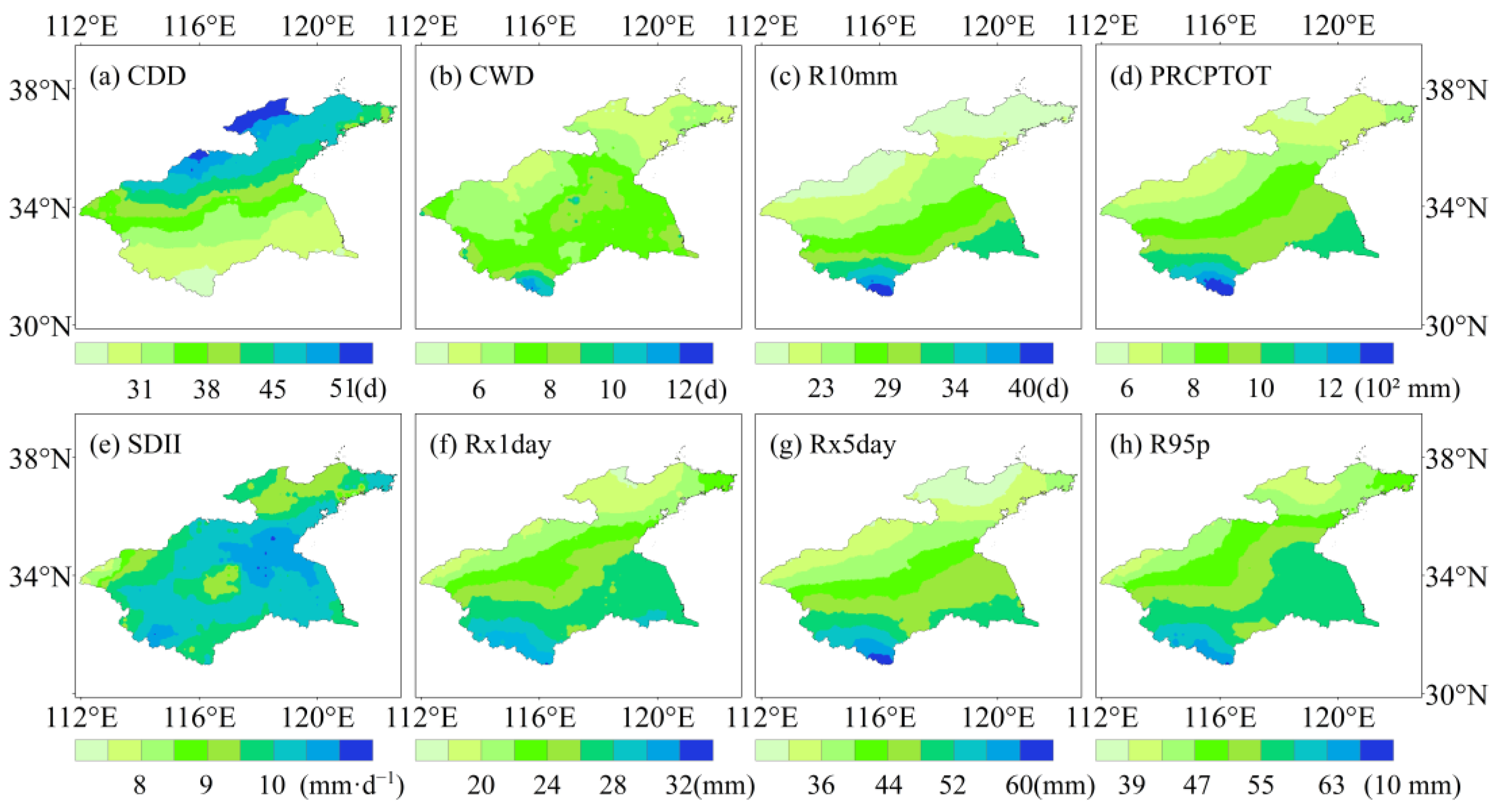
The spatial distribution of climatological means of different indices from 1961 to 2020 is shown in Figure 2. Except for SDII and CDD, all other indices show a comparable spatial pattern for the climatological means. Generally, higher values are observed in the southwest region of the basin, gradually decreasing towards the northern portion. Notably, CDD demonstrates a more pronounced distribution, with higher values concentrated north of 34 °N in the basin and having a clear declining tendency from northwest to southeast. SDII exhibits mild spatial variability, with the lowest values (7.320 mm d−1) in the western mountainous region and a regional center of high value (11.110 mm d−1) in the middle and lower portions of the basin.
Subtle variations can be observed in the spatial patterns of several extreme precipitation indices, as shown in Figure 3. Approximately 86% of the study area exhibits an upward trend in PRCPTOT, with significant increases centered in the southwest of the basin at a 95% confidence level, while no significant decreases are observed. SDII shows growth in the central area with declining tendencies in the peripheral regions, particularly in the northern section of the basin. The distribution patterns of SDII and CDD are similar. Moreover, CWD is becoming more prominent in the eastern coastal regions and western highland areas, while declining in other locations.
The analysis of the eight aforementioned extreme precipitation indices reveals that the spatiotemporal patterns, particularly for indices such as SDII, Rx1day, and Rx5day that are linked to intensity, are strongly influenced by topography. Therefore, taking models’ simulation capabilities of spatial pattern into consideration is essential when conducting the model assessment.

3.2. Assessment of Model Performance for Extreme Precipitation Indices

The results shown in Figure 2 and Figure 3 demonstrate a pronounced spatial non-uniformity in extreme precipitation, which is consistent with previous studies [81,82]. The assessment concentrates on the spatial distribution of climatological means and trends for each index during the historical period from 1995 to 2014 to gauge the model’s performance. Here, the average of meteorological variables recorded between 1995 and 2014 is referred to as the climatological means.
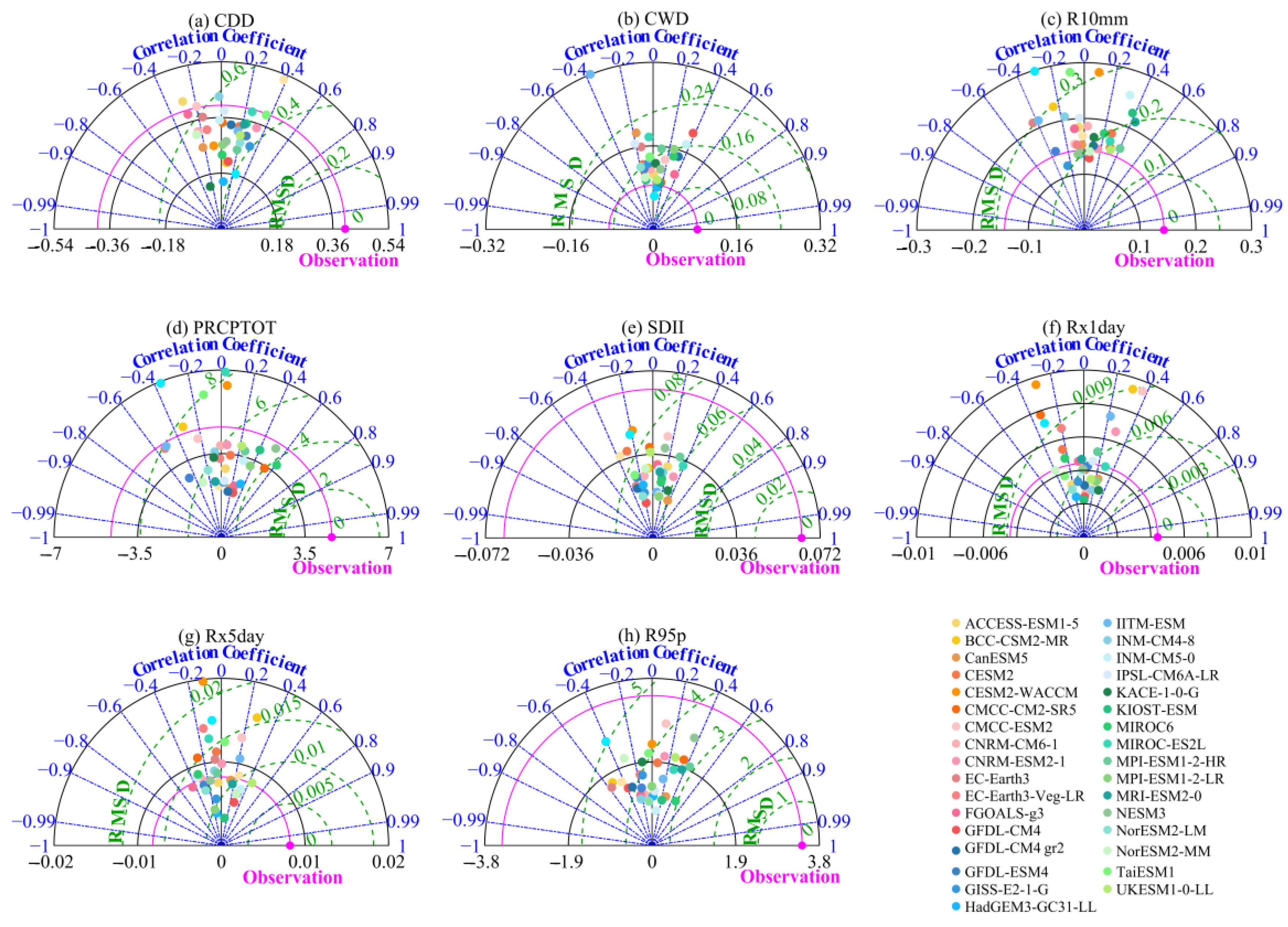
The Taylor diagram shown in Figure 4 offers an analysis of spatial distribution of trends in extreme precipitation indices for the years 1995 to 2014. It reveals that a significant number of models exhibit weak correlations when it comes to specific extreme precipitation indices. Among these, the CMCC-CM2-SR5 model exhibits the strongest correlation in the trend of total precipitation (PRCPTOT), albeit still being below 0.590. The ratio of the model’s standard deviation (SDmodel) to the observed standard deviation (SDobs) ranges from 0.230 to 3.790. The normalized RSME, defined as the ratio of the RSME to the SDobs, is concentrated between 0.800 and 2.500. These results indicate that the models have a limited ability to capture the spatial patterns of trend changes, which requires further improvements in their performance. It is worth noting that the resolution of the models significantly affects their performance, and downscaled climate models are still insufficient in the simulation of extreme precipitation indices in the humid regions of eastern China. Therefore, apart from resolution, other factors such as the dynamic framework of the models require further investigation to better replicate the complex spatial characteristics of extreme precipitation. Simulating longer-term climate sequences often results in greater modeling performance. The length of the simulated period is another significant component that impacts the modeling capacity [31,83]. This finding provides insight into one possible explanation for the weak correlation between the observed data and the models, in addition to the inherent limitations in the accuracy of the models.
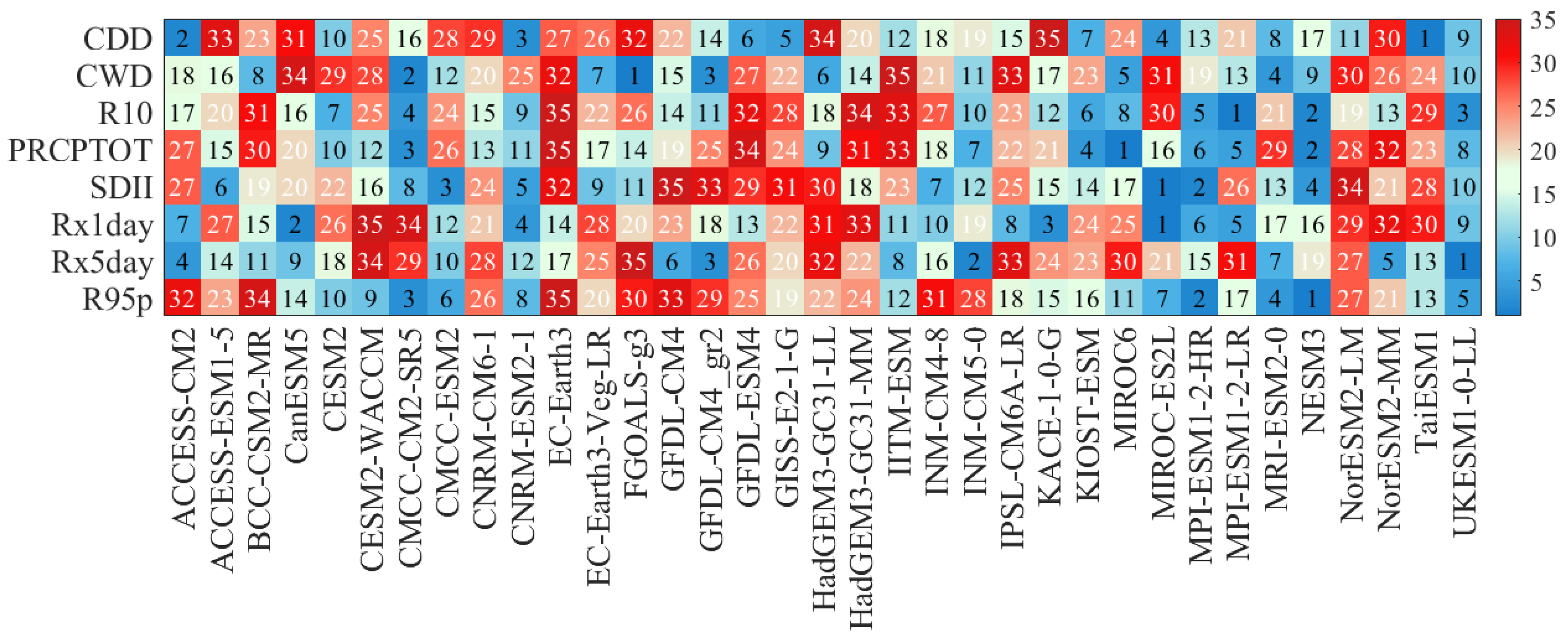
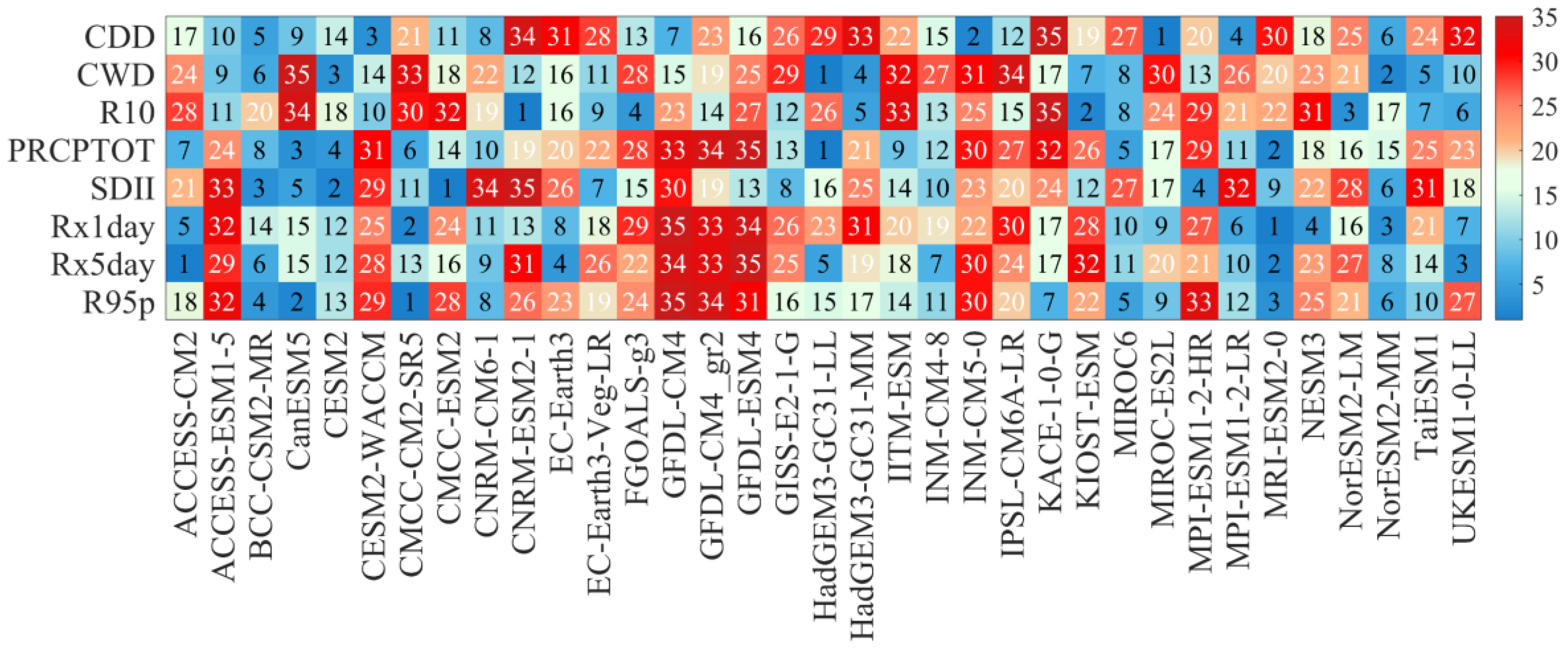
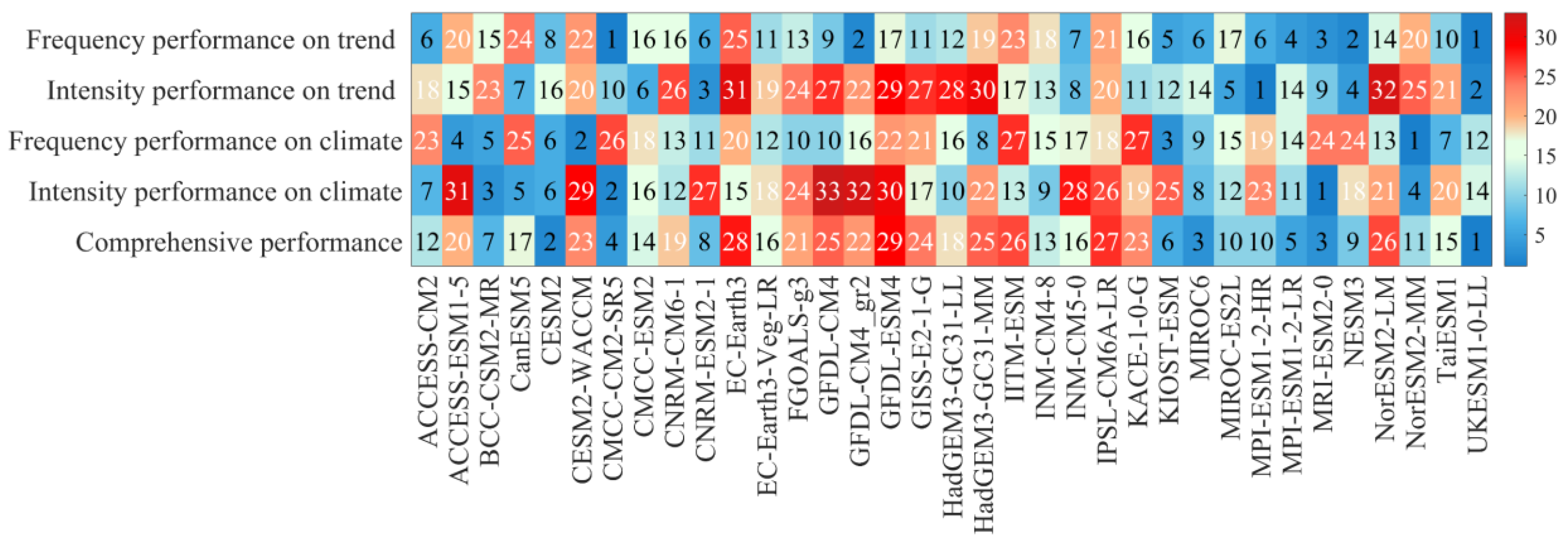
Based on the analysis depicted in Figure 4, the TS values were calculated for the various indices across the 35 models, and then a unique ranking was established as shown in Figure 5. The findings clearly indicate significant disparities in the modeling performance among the different models. For example, KACE-1-0-G exhibits the weakest performance in simulating the CDD index, while closely trailing the top-performing models, MIROC-ES2L and CanESM5, for the Rx1day index. In terms of overall performance, UKESM1-0-LL, CMCC-CM2-SR5, and GFDL-CM4_gr2 perform better for frequency indices and MPI-ESM1-2-HR and UKESM1-0-LL exhibit superior performance for intensity indices. By leveraging the ensemble mean of better-performing models, researchers improve the analysis of extreme precipitation trends, leading to more reliable and integrated results in assessing the regional impacts of climate change.
The distribution of climatological means of each model exhibits a high level of agreement with observed precipitation, indicating successful simulation (Figure 6 and Figure 7). For the PRCPTOT, which represents the integrated changes in precipitation, models show the highest R values exceeding 0.850. The ratio of RMSE to SDobs generally remains below 0.500, and the ratio of SD spans from 0.800 to 1.250, closely approximating the spatial patterns of observed precipitation. The Taylor plots show the distribution of climate models is organized, indicating a high degree of agreement among them. They perform relatively better in simulating the Rx5day and R95p indices, while improvements are still needed for accurate simulation of SDII and CWD. All models consistently underestimate Rx1day and Rx5day, while overestimating CWD and R10mm. These biases exhibit a strong correlation with topography, where increased topographical complexity leads to larger discrepancies [84,85]. More specifically, smaller biases are observed in the central plain regions of the basin, while the western mountainous areas and eastern coastal regions of the basin show more significant disparities. When using datasets in areas with complicated topography, it is necessary to employ appropriate bias correction techniques. Furthermore, it is important to acknowledge that the model’s ability to simulate extreme precipitation indices is subject to significant uncertainty, which can be influenced by various factors such as structural frameworks, external forcing, and other considerations.

3.3. Assessment of Preferred Models

Since there is significant regional variability in extreme precipitation, reliable data are crucial for predicting regional dangers that are involved. A large number of researchers mainly use data from CMIP models to forecast extreme precipitation events, which means the success of related risk evaluation efforts is directly influenced by the models’ ability to simulate the observational data. So, selecting appropriate simulation outcomes from a wide array of models is critical. To further pinpoint models with the best simulation ability, the spatial distribution of trends and the horizontal pattern of climatological means were assessed in terms of how they reproduce real-world conditions accurately (Figure 8), using an extensive ranking method.
The analysis of extreme precipitation indices in many studies is mainly attributed to frequency, intensity, area, and duration. In this work, the eight extreme precipitation indices are separated into two groups, according to their definitions: frequency index (CDD, CWD, R10mm) and intensity index (PRCPTOT, SDII, Rx1day, Rx5day, R95p). The ability of 35 models to replicate extreme precipitation is thoroughly examined in terms of climate, tendency, and the combination of the two, using the Mr scores. Figure 8 demonstrates that most models that underperform in simulating intensity tend to perform better in simulating frequency. Meanwhile, models weaker in capturing trends often exhibit better simulation skills in representing climatological means. Contrary to the assessment of extreme temperature, this pattern introduces a higher amount of uncertainty [86,87]. For instance, CMCC-CM2-SR5 is ranked 26th in terms of simulating frequency indices in time changes, but demonstrates competitive performance in simulating the climatological means of intensity indices, coming in second place to MRI-ESM2-0. Certain models demonstrated strong simulation capability for both extreme frequency and intensity indices, encompassing both climatological means and tendency. UKESM1-0-LL performs the best among all considered models, also showing high simulation abilities across other evaluation measures [88]. This finding indicates that UKESM1-0-LL has the best ability to simulate extreme precipitation events over the HRB. In general, UKESM1-0-LL, CESM2, MIROC6, MRI-ESM2-0, CMCC-CM2-SR5, and MPI-ESM-2-LR exhibit superior simulation capabilities, consistently ranking in the top five models. Among these, MIROC6 and MRI-ESM2-0 are both ranked third.
Researchers commonly use multi-model ensemble averaging to reduce uncertainties in extreme weather/climate events projection. However, a single model with substantial deviations may introduce more errors and uncertainties. Therefore, we selected the top five models with excellent simulation capabilities, i.e., the Mr scores exceed 0.680, as our final preferred models, referring to the Reference [80]. We derived a weighted average of the six favored models based on the Mr scores. Mr scores for UKESM1-0-LL, CESM2, MIROC6, MRI-ESM2-0, CMCC-CM2-SR5, and MPI-ESM-2-LR are 0.793, 0.743, 0.736, 0.736, 0.721, and 0.700, respectively. As a result, their weights are 0.179, 0.168, 0.166, 0.163, and 0.157, respectively, according to Equation (11).
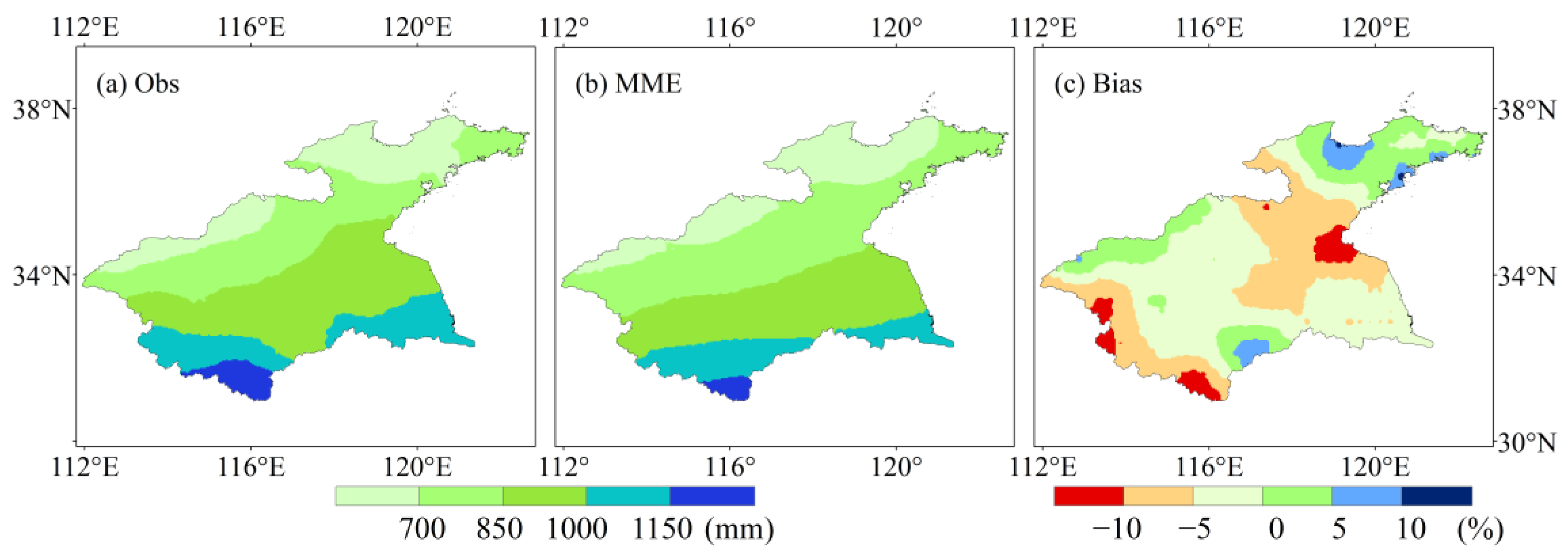
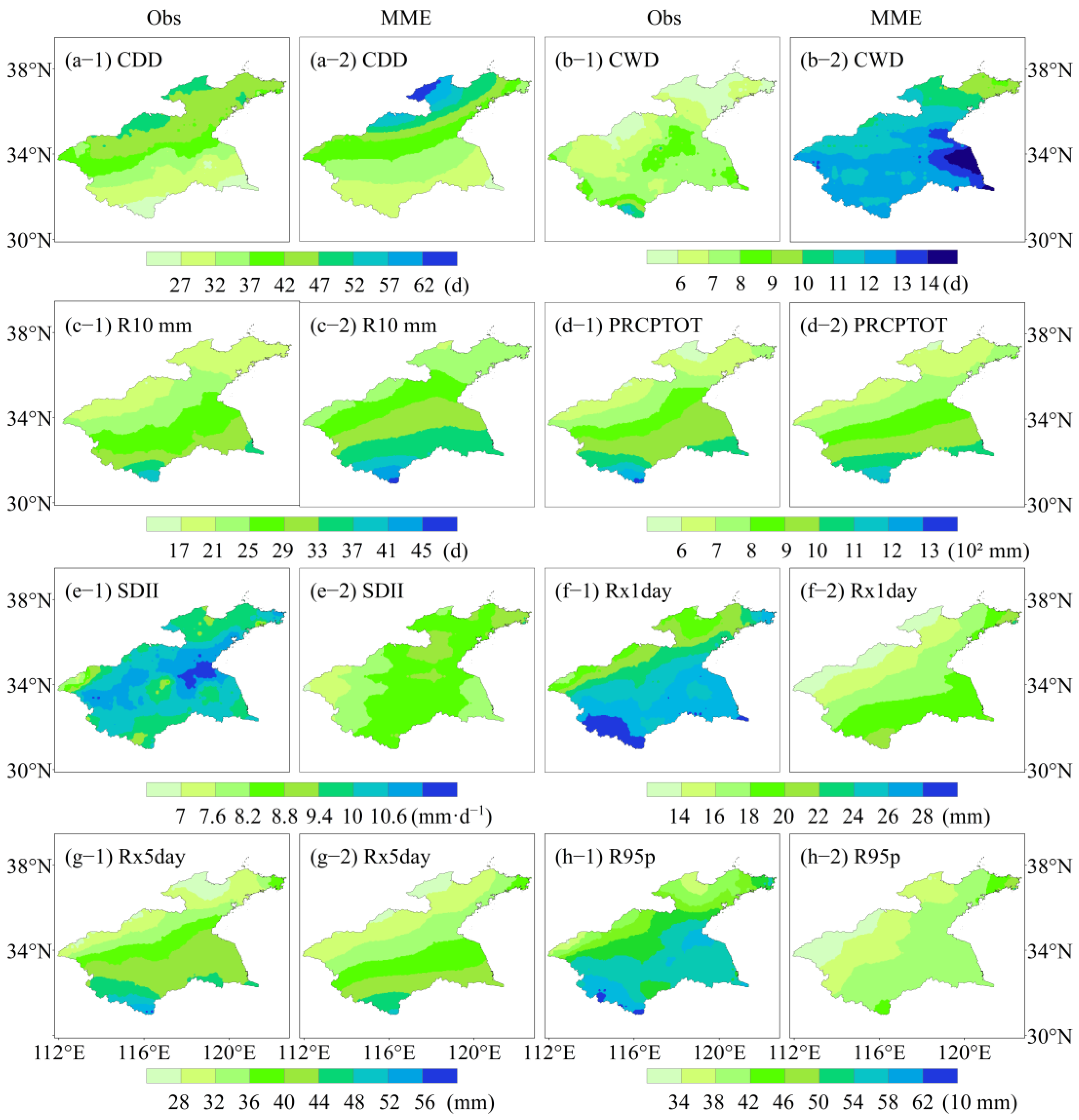
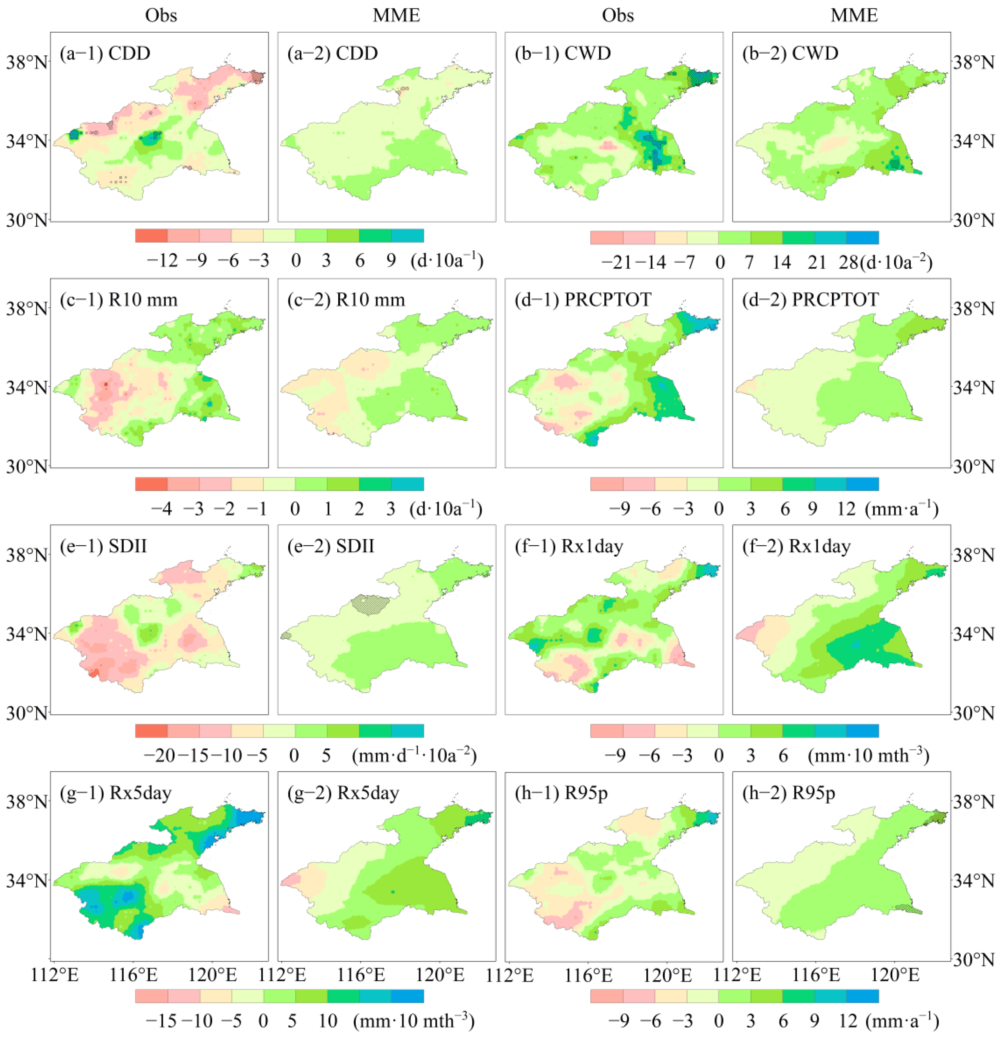
The preferred models’ ensemble has a slight bias of less than 10% relative to the annual precipitation perspective (Figure 9), successfully reproducing the spatial distribution pattern of a decreasing trend from southeast to northwest over the HRB. Although the ensemble tends to underestimate indices such as Rx1day, R95p, and SDII when taking into account the climatological means and trend fluctuations, as illustrated in Figure 10 and Figure 11, the discrepancies in magnitude are typically negligible. Additionally, the ensemble appropriately depicts the steady trends of the R10mm, Rx1day, and Rx5day indices across the entire basin, as well as the distribution characteristics of indices such as CDD, PRCPTOT, and Rx5day. As a result, it can be said that the ensemble of the recommended models is an effective instrument for faithfully modeling extreme precipitation over the HRB.
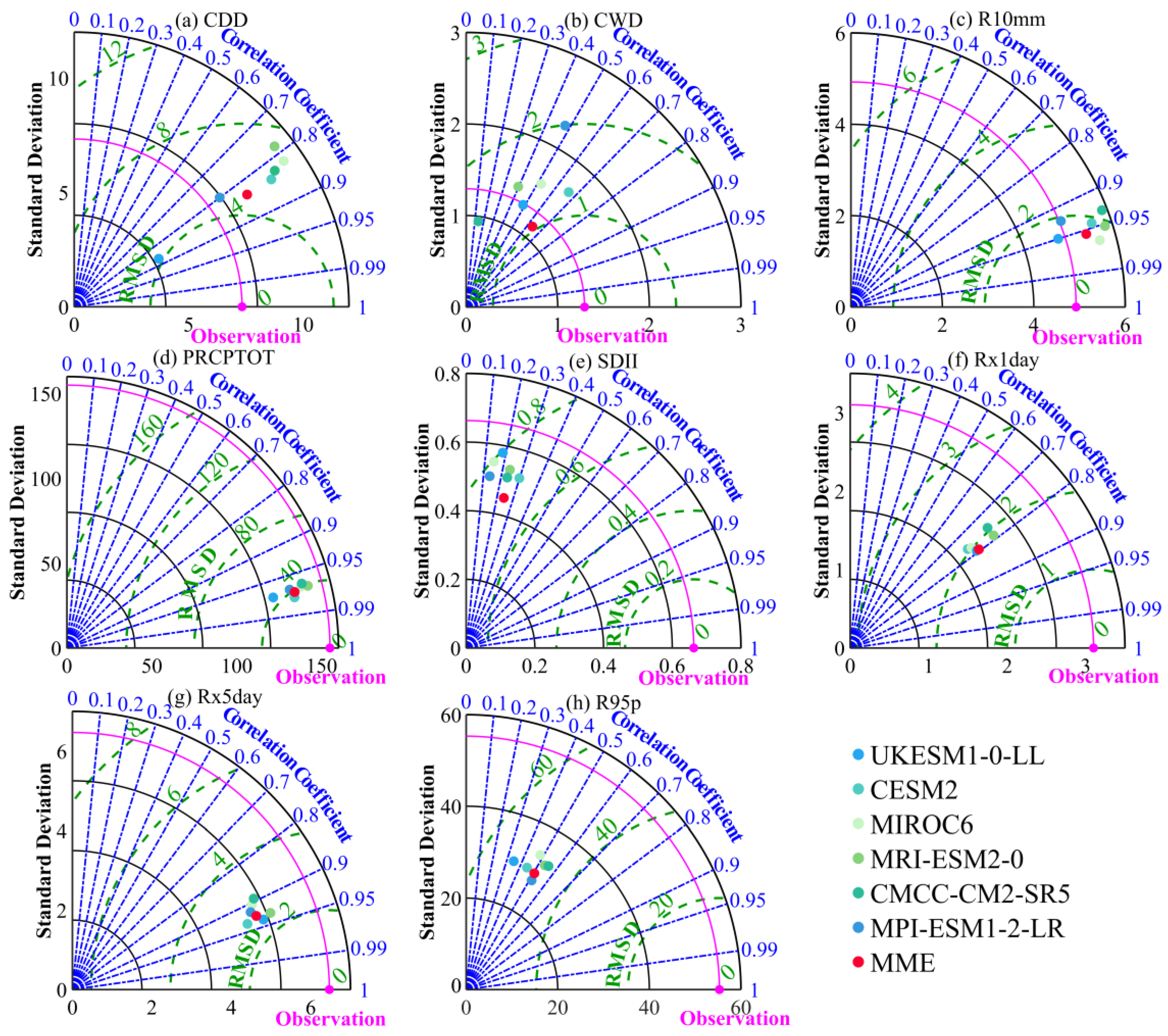
According to the Taylor diagram (Figure 12 and Figure 13), the ensemble greatly improves the negative correlation that individual models showed across many indices and exhibits greater precipitation-catching abilities. The ensemble shows enhanced comprehensive modeling skills for frequency indices such as CDD, CWD, and R10mm with excellent spatial correlation coefficients. Furthermore, in comparison to the observed values, R10mm and Rx5day both exhibit significant spatial correlation coefficients that exceed 0.900. With an average climatological correlation coefficient for the eight indices of 0.800, the ensemble of preferred models performs best when compared to individual models and the ensemble mean of all models.
Consequently, using the ensemble mean of the selected models is a more reliable and justifiable strategy in the scientific study of the estimation of future extreme precipitation-related disaster risks over the HRB.

4. Discussion

The inherent, non-uniform characteristics of extreme precipitation have caused strong biases between models and observational data. Furthermore, the HRB is located in the East Asian Monsoon Zone of China, where precipitation caused by the East Asian Monsoon during summer plays a significant role in driving regional extreme precipitation [22]. That is, the unique location and climate mechanism of the HRB further enlarge the uneven features of extreme precipitation. Moreover, the eastern region has experienced significant economic development, resulting in increased human activities that have intensified the impact on the environment surrounding meteorological observation stations. This has led to the observed values deviating from the actual, true values. The primary basis for modulating the model outputs is the observed data, which, to some extent, adds to the modeling discrepancies [31]. It is worth noting that the biases are relatively small in absolute magnitude, indicating that it is reasonable to see variations in the model’s capacity to replicate the precipitation’s spatiotemporal trends.
Previous research has also demonstrated that the CMIP6 data, which provide higher resolution and higher fidelity, are a trustworthy source for climate studies. Compared to CMIP5, the data show significant improvements in simulating extreme precipitation in arid and semi-arid regions, but with less significant improvements in the humid parts of eastern China [87]. Inaccuracies can also be seen in the data of NEX-GDDP-CMIP6, a downscaled version of CMIP6, in capturing the eastern region’s precipitation characteristics. There is a greater need for models to meet stricter performance requirements due to the complex, interrelated processes that affect the climatic patterns in the eastern monsoon zone. Therefore, additional research is required to explore the model’s physical processes, dynamic frameworks, and other pertinent factors aside from resolution concerns in order to better comprehend its potential in simulation.
It is important to recognize the uncertainties and restrictions related to this study. The choice and combination of indicators can have an impact on the results of the assessment. There are inherent limitations in using eight frequently used extreme precipitation indices to assess the capabilities of simulating extreme precipitation frequency and intensity. Furthermore, China’s vast geographical expanse gives rise to potential disparities in the simulation performance of a single climate model across different topographical regions. UKESM1-0-LL is the model that performs the best overall in our thorough evaluation of the whole HRB, and MIROC6 was the model that performed the best in the study conducted by Li et al. [89], which considered the integrity of administrative units to divide the HRB. One potential explanation for these discrepancies lies in the inherent differences in physical parameters, system configurations, and other model-specific attributes among the various climate models. These distinctions could account for variations in their capacity to capture precipitation patterns across diverse topographic regions. Consequently, a more in-depth analysis and investigation into the sources of errors among these models is imperative. Additionally, there are may still some outliers in the outputs due to the model’s physical parameter settings and potential biases inherited from the driving GCMs. However, the number of outliers is minimal in comparison to the whole data sample and is ignored throughout processing. These ignored outliers may, to some extent, lead to inaccuracies in the climate model performance, which will influence model selection and potentially lead to significant errors in the preferred multi-model means. Therefore, it is crucial to identify such outliers and address them scientifically [90]. In future work, it may be worthwhile to delve into this aspect by, for instance, performing sensitivity analysis of outliers, determining whether outliers have a significant impact on model assessments, or considering the use of the entire ensemble climate sensitivity range to account for uncertainties in future climates. The model ensemble employed a straightforward weighted average method based on Mr scores, and future research could explore more sophisticated weighted ensemble methods that take into account more variables. It would also be worthwhile to conduct further research into the application of various evaluation techniques to reduce model uncertainty.

5. Conclusions

This study evaluates 35 NEX-GDDP climate models’ performance in simulating extreme precipitation events in the HRB using eight specific indicators. The results can be concluded as follows:
(1)
The underlying topography and the spatial dynamics of extreme precipitation indices over the HRB are well related. Both frequency and intensity indices exhibit noticeable variations in regions with significant changes in the topography, which emphasizes the need for climate models to accurately replicate the complex spatial features linked to these indices.
(2)
The models’ capacity to replicate the trends of extreme precipitation requires further development. With a positive correlation with the observed field in 87% of the extreme precipitation indices, UKESM1-0-LL outperforms the other considered models, but still with a relatively weak connection. Since different models exhibit large differences in their capacity to represent both the trends and climatology of various indices, a great deal of uncertainty is introduced into the simulation of extreme precipitation indices. In comparison to their trend simulations, models perform better when modeling the climatological means, and they are better at simulating frequency indices than intensity indices. NorESM2-MM and MRI-ESM2-0, in particular, are excellent at simulating climatology. UKESM1-0-LL, CMCC-CM2-SR5, and MPI-ESM1-2-HR have relatively superior performance in terms of changing trends.
(3)
Based on their comparatively superior simulation abilities, the preferred models, UKESM1-0-LL, CESM2, MIROC6, MRI-ESM2-0, CMCC-CM2-SR5, and MPIESMI-2-LR, were ultimately chosen. Only a few of these models’ ensembles deviate from the observed data, primarily in the western mountains. Additionally, the contribution rate of the deviation varies very little between the eastern, central, and western regions. The models’ performances for frequency indices show strong agreement with the spatial pattern of the observed climate, and the negative correlations in the temporal patterns of intensity indices are significantly mitigated. To put it another way, the ensemble of selected models shows some degree of applicability.
In conclusion, the NEX-GDDP-CMIP6 dataset exhibits some degree of reliability over the HRB. The high-resolution downscaled datasets are expected to be used widely as research into climate change advances and demands for risk and catastrophe mitigation rise. Our findings establish a scientific foundation for decision making concerning climate change mitigation and adaptation, and serve as a basis for model selection in estimating risks associated with extreme precipitation occurrences. Furthermore, the thorough evaluation of the simulation capabilities of the NEX-GDDP-CMIP6 climate models over the HRB not only aids in better understanding and utilization of these climate models, but also provides theoretical support for their advancement. It also offers theories and methods for studying extreme precipitation in various geographic areas, which is crucial in areas with complicated climatic causes or transitional climate zones.

Author Contributions

Conceptualization, S.W., M.G. and A.Z.; Writing—original draft, F.J.; Writing—review and editing, S.W. All authors have read and agreed to the published version of the manuscript.

Funding

This study was supported by the National Natural Science Foundation of China (42005126).

Institutional Review Board Statement

Not applicable.

Informed Consent Statement

Not applicable.

Data Availability Statement

Not applicable.

Conflicts of Interest

The authors declare no conflict of interest.

References

  1. Dessler, A.E.; Schoeberl, M.R.; Wang, T.; Davis, S.M.; Rosenlof, K.H. Stratospheric water vapor feedback. Proc. Natl. Acad. Sci. USA 2013, 110, 18087–18091. [Google Scholar] [CrossRef]
  2. Burke, C.; Stott, P.; Ciavarella, A.; Sun, Y. Attribution of Extreme Rainfall in Southeast China During May 2015. Bull. Am. Meteorol. Soc. 2016, 97, S92–S96. [Google Scholar] [CrossRef]
  3. Chen, H.; Sun, J. Changes in climate extreme events in China associated with warming. Int. J. Climatol. 2015, 35, 2735–2751. [Google Scholar] [CrossRef]
  4. Huo, R.; Li, L.; Chen, H.; Xu, C.Y.; Chen, J.; Guo, S. Extreme Precipitation Changes in Europe from the Last Millennium to the End of the Twenty-First Century. J. Clim. 2021, 34, 567–588. [Google Scholar] [CrossRef]
  5. Shenoy, S.; Gorinevsky, D.; Trenberth, K.E.; Chu, S. Trends of extreme US weather events in the changing climate. Proc. Natl. Acad. Sci. USA 2022, 119, e2207536119. [Google Scholar] [CrossRef] [PubMed]
  6. IPCC. AR6 Climate Change 2021: The Physical Science Basis; Contribution of Working Group I to the Sixth Assessment Report of the Intergovernmental Panel on Climate Change; Cambridge University Press: Cambridge, UK, 2021. [Google Scholar]
  7. Jiang, T.; Su, B.; Huang, J.; Zhai, J.; Xia, J.; Tao, H.; Wang, Y.; Su, H.; Luo, Y.; Zhang, L.; et al. Each 0.5 °C of Warming Increases Annual Flood Losses in China by More than US$60 Billion. Bull. Am. Meteorol. Soc. 2020, 101, E1464–E1474. [Google Scholar] [CrossRef]
  8. Zhang, W.; Zhou, T. Increasing impacts from extreme precipitation on population over China with global warming. Sci. Bull. 2020, 65, 243–252. [Google Scholar] [CrossRef]
  9. Hirabayashi, Y.; Tanoue, M.; Sasaki, O.; Zhou, X.; Yamazaki, D. Global exposure to flooding from the new CMIP6 climate model projections. Sci. Rep. 2021, 11, 3740. [Google Scholar] [CrossRef]
  10. Cook, B.I.; Mankin, J.S.; Marvel, K.; Williams, A.P.; Smerdon, J.E.; Anchukaitis, K.J. Twenty-first century drought projections in the CMIP6 forcing scenarios. Earth's Future 2020, 8, e2019EF001461. [Google Scholar] [CrossRef]
  11. Wang, B.; Jin, C.; Liu, J. Understanding Future Change of Global Monsoons Projected by CMIP6 Models. J. Clim. 2020, 33, 6471–6489. [Google Scholar] [CrossRef]
  12. Eyring, V.; Bony, S.; Meehl, G.A.; Senior, C.A.; Stevens, B.; Stouffer, R.J.; Taylor, K.E. Overview of the Coupled Model Intercomparison Project Phase 6 (CMIP6) experimental design and organization. Geosci. Model Dev. 2015, 9, 1937–1958. [Google Scholar] [CrossRef]
  13. Zhou, T.J.; Zhou, L.W.; Chen, X.L. Commentary on the coupled model intercomparison project phase 6 (CMIP6). Adv. Clim. Chang. Res. 2019, 15, 445–456. (In Chinese) [Google Scholar]
  14. Chen, H.; Sun, J.; Lin, W.; Xu, H. Comparison of CMIP6 and CMIP5 models in simulating climate extremes. Sci. Bull. 2020, 65, 1415–1418. [Google Scholar] [CrossRef] [PubMed]
  15. Zhu, H.; Jiang, Z.; Li, L. Projection of climate extremes in China, an incremental exercise from CMIP5 to CMIP6. Sci. Bull. 2021, 66, 2528–2537. [Google Scholar] [CrossRef]
  16. Kim, Y.H.; Min, S.K.; Zhang, X.; Sillmann, J.; Sandstad, M. Evaluation of the CMIP6 multi-model ensemble for climate extreme indices. Weather Clim. Extrem. 2020, 29, 100269. [Google Scholar] [CrossRef]
  17. Li, Y.; Yan, D.; Peng, H.; Xiao, S. Evaluation of precipitation in CMIP6 over the Yangtze River Basin. Atmos. Res. 2020, 253, 105406. [Google Scholar] [CrossRef]
  18. Gu, X.; Ye, L.; Xin, Q.; Zhang, C.; Zeng, F.; Nerantzaki, S.D.; Papalexiou, S.M. Extreme Precipitation in China: A Review on Statistical Methods and Applications. Adv. Water Resour. 2022, 163, 104144. [Google Scholar] [CrossRef]
  19. Wu, G.; Li, J.; Zhou, T.; Lu, R.; Yu, Y.; Zhu, J.; Mu, M. CMIP. Adv. Earth Sci. 2006, 21, 1109. [Google Scholar]
  20. Kailin, Y.; Miao, Y.; Li, G.; Hong, L. Relationships Between Precipitation Anomaly in Meiyu Period in the Yangtze-Huaihe Region and Surface Sensible Heat Flux over East Asia. J. Arid Meteorol. 2019, 37, 771. [Google Scholar]
  21. Yin, Y.; Chen, H.; Zhai, P.; Xu, C.Y.; Ma, H. Characteristics of summer extreme precipitation in the Huai River basin and their relationship with East Asia summer monsoon during 1960–2014. Int. J. Climatol. 2019, 39, 1555–1570. [Google Scholar] [CrossRef]
  22. Sun, Q.; Miao, C. Extreme Rainfall (R20mm, RX5day) in Yangtze–Huai, China, in June–July 2016: The Role of ENSO and Anthropogenic Climate Change. Bull. Am. Meteorol. Soc. 2018, 99, S102–S106. [Google Scholar] [CrossRef]
  23. Chen, F.; Zheng, X.; Wen, H.; Yuan, Y. Microphysics of Convective and Stratiform Precipitation during the Summer Monsoon Season over the Yangtze–Huaihe River Valley, China. J. Hydrometeorol. 2022, 23, 239–252. [Google Scholar] [CrossRef]
  24. Liu, J.; Zhang, B.; Yao, Y.; Zhang, X.; Wang, J.; Yu, F.; Li, J. Latitudinal differentiation and patterns of temperate and subtropical plants in the Qinling-Daba Mountains. J. Geogr. Sci. 2023, 33, 907–923. [Google Scholar] [CrossRef]
  25. Sun, Y.; Ding, Y. A projection of future changes in summer precipitation and monsoon in East Asia. Sci. China Earth Sci. 2010, 53, 284–300. [Google Scholar] [CrossRef]
  26. Li, Z.; Sun, Y.; Li, T.; Ding, Y.; Hu, T. Future changes in East Asian summer monsoon circulation and precipitation under 1.5 to 5 C of warming. Earth's Future 2019, 7, 1391–1406. [Google Scholar]
  27. Li, X.; Fang, G.; Wei, J.; Arnault, J.; Laux, P.; Wen, X.; Kunstmann, H. Evaluation and projection of precipitation and temperature in a coastal climatic transitional zone in China based on CMIP6 GCMs. Clim. Dyn. 2023, 61, 1–23. [Google Scholar] [CrossRef]
  28. Mou, S.; Shi, P.; Qu, S.; Feng, Y.; Chen, C.; Dong, F. Projected regional responses of precipitation extremes and their joint probabilistic behaviors to climate change in the upper and middle reaches of Huaihe River Basin, China. Atmos. Res. 2020, 240, 104942. [Google Scholar] [CrossRef]
  29. Jin, H.; Chen, X.; Zhong, R.; Duan, K. Frequency analysis of extreme precipitation in different regions of the Huaihe River Basin. Int. J. Climatol. 2021, 42, 3517–3536. [Google Scholar] [CrossRef]
  30. Wang, Y.; Wang, Y.; Wang, Y.; Ju, Q.; Jin, J.; Bao, Z. Projecting Changes in Rainfall Extremes for the Huai River Basin in the Context of 1.5 °C and 2 °C Global Warming. Atmosphere 2022, 13, 1708. [Google Scholar] [CrossRef]
  31. Wu, Y.; Miao, C.; Duan, Q.; Shen, C.; Fan, X. Evaluation and projection of daily maximum and minimum temperatures over China using the high-resolution NEX-GDDP dataset. Clim. Dyn. 2020, 55, 2615–2629. [Google Scholar] [CrossRef]
  32. Thrasher, B.; Wang, W.; Michaelis, A.; Melton, F.; Lee, T.; Nemani, R. NASA Global Daily Downscaled Projections, CMIP6. Sci. Data 2022, 9, 262. [Google Scholar] [CrossRef]
  33. Chen, H.P.; Sun, J.Q.; Li, H.X. Future changes in precipitation extremes over China using the NEX-GDDP high-resolution daily downscaled data-set. Atmos. Ocean. Sci. Lett. 2017, 10, 403–410. [Google Scholar] [CrossRef]
  34. Zhang, Y.; You, Q.; Ullah, S.; Chen, C.; Shen, L.; Liu, Z. Substantial increase in abrupt shifts between drought and flood events in China based on observations and model simulations. Sci. Total Environ. 2023, 876, 162822. [Google Scholar] [CrossRef] [PubMed]
  35. Xu, L.; Zhang, T.; Yu, W.; Yang, S. Changes in concurrent precipitation and temperature extremes over the Asian monsoon region: Observation and projection. Environ. Res. Lett. 2023, 18, 044021. [Google Scholar] [CrossRef]
  36. Qin, Z.; Zhao, J.; Cheng, W.X.; Wang, J.; Su, H.L.; He, Y.L. Change of subtropical northern boundary in Qinling− Huaihe region in the context of climate change. Adv. Clim. Chang. Res. 2023, 19, 38–48. (In Chinese) [Google Scholar]
  37. Cao, Q.; Hao, Z.; Yuan, F.; Berndtsson, R.; Xu, S.; Gao, H.; Hao, J. On the predictability of daily rainfall during rainy season over the Huaihe River Basin. Water 2019, 11, 916. [Google Scholar] [CrossRef]
  38. Dai, C.; Qin, X.; Lu, W.; Huang, Y. Assessing adaptation measures on agricultural water productivity under climate change: A case study of Huai River Basin, China. Sci. Total Environ. 2020, 721, 137777. [Google Scholar] [CrossRef]
  39. Wu, J.; Gao, X.J. A gridded daily observation dataset over China region and comparison with the other datasets. Chin. J. Geophys. Chin. Ed. 2013, 56, 1102–1111. (In Chinese) [Google Scholar]
  40. Sun, B.; Wang, H. Enhanced connections between summer precipitation over the Three-River-Source region of China and the global climate system. Clim. Dyn. 2019, 52, 3471–3488. [Google Scholar] [CrossRef]
  41. Song, Z.; Xia, J.; She, D.; Li, L.; Hu, C.; Hong, S. Assessment of meteorological drought change in the 21st century based on CMIP6 multi-model ensemble projections over mainland China. J. Hydrol. 2021, 601, 126643. [Google Scholar] [CrossRef]
  42. Wood, A.W.; Maurer, E.P.; Kumar, A.; Lettenmaier, D.P. Long-range experimental hydrologic forecasting for the eastern United States. J. Geophys. Res. Atmos. 2002, 107, ACL 6-1–ACL 6-15. [Google Scholar] [CrossRef]
  43. Wood, A.W.; Leung, L.R.; Sridhar, V.; Lettenmaier, D.P. Hydrologic Implications of Dynamical and Statistical Approaches to Downscaling Climate Model Outputs. Clim. Chang. 2004, 62, 189–216. [Google Scholar] [CrossRef]
  44. Bi, D.; Dix, M.; Marsland, S.; O’farrell, S.; Sullivan, A.; Bodman, R.; Law, R.; Harman, I.; Srbinovsky, J.; Rashid, H.A. Configuration and spin-up of ACCESS-CM2, the new generation Australian community climate and earth system simulator coupled model. J. South. Hemisph. Earth Syst. Sci. 2020, 70, 225–251. [Google Scholar] [CrossRef]
  45. Ziehn, T.; Chamberlain, M.A.; Law, R.M.; Lenton, A.; Bodman, R.W.; Dix, M.; Stevens, L.; Wang, Y.P.; Srbinovsky, J. The Australian earth system model: : ACCESS-ESM1. 5. J. South. Hemisph. Earth Syst. Sci. 2020, 70, 193–214. [Google Scholar] [CrossRef]
  46. Wu, T.; Lu, Y.; Fang, Y.; Xin, X.; Li, L.; Li, W.; Jie, W.; Zhang, J.; Liu, Y.; Zhang, L. The Beijing Climate Center climate system model (BCC-CSM): The main progress from CMIP5 to CMIP6. Geosci. Model Dev. 2019, 12, 1573–1600. [Google Scholar] [CrossRef]
  47. Swart, N.C.; Cole, J.N.; Kharin, V.V.; Lazare, M.; Scinocca, J.F.; Gillett, N.P.; Anstey, J.; Arora, V.; Christian, J.R.; Hanna, S. The Canadian earth system model version 5 (CanESM5. 0.3). Geosci. Model Dev. 2019, 12, 4823–4873. [Google Scholar] [CrossRef]
  48. Danabasoglu, G.; Lamarque, J.F.; Bacmeister, J.; Bailey, D.; DuVivier, A.; Edwards, J.; Emmons, L.; Fasullo, J.; Garcia, R.; Gettelman, A. The community earth system model version 2 (CESM2). J. Adv. Model. Earth Syst. 2020, 12, e2019MS001916. [Google Scholar] [CrossRef]
  49. Gettelman, A.; Mills, M.; Kinnison, D.; Garcia, R.; Smith, A.; Marsh, D.; Tilmes, S.; Vitt, F.; Bardeen, C.; McInerny, J. The whole atmosphere community climate model version 6 (WACCM6). J. Geophys. Res. Atmos. 2019, 124, 12380–12403. [Google Scholar] [CrossRef]
  50. Cherchi, A.; Fogli, P.G.; Lovato, T.; Peano, D.; Iovino, D.; Gualdi, S.; Masina, S.; Scoccimarro, E.; Materia, S.; Bellucci, A. Global mean climate and main patterns of variability in the CMCC-CM2 coupled model. J. Adv. Model. Earth Syst. 2019, 11, 185–209. [Google Scholar] [CrossRef]
  51. Lovato, T.; Peano, D.; Butenschön, M.; Materia, S.; Iovino, D.; Scoccimarro, E.; Fogli, P.; Cherchi, A.; Bellucci, A.; Gualdi, S. CMIP6 simulations with the CMCC Earth system model (CMCC-ESM2). J. Adv. Model. Earth Syst. 2022, 14, e2021MS002814. [Google Scholar] [CrossRef]
  52. Voldoire, A.; Saint-Martin, D.; Sénési, S.; Decharme, B.; Alias, A.; Chevallier, M.; Colin, J.; Guérémy, J.F.; Michou, M.; Moine, M.P. Evaluation of CMIP6 deck experiments with CNRM-CM6-1. J. Adv. Model. Earth Syst. 2019, 11, 2177–2213. [Google Scholar] [CrossRef]
  53. Séférian, R.; Nabat, P.; Michou, M.; Saint-Martin, D.; Voldoire, A.; Colin, J.; Decharme, B.; Delire, C.; Berthet, S.; Chevallier, M. Evaluation of CNRM Earth System Model, CNRM-ESM2-1: Role of Earth system processes in present-day and future climate. J. Adv. Model. Earth Syst. 2019, 11, 4182–4227. [Google Scholar] [CrossRef]
  54. Döscher, R.; Acosta, M.; Alessandri, A.; Anthoni, P.; Arneth, A.; Arsouze, T.; Bergmann, T.; Bernadello, R.; Bousetta, S.; Caron, L.P. The EC-earth3 Earth system model for the climate model intercomparison project 6. Geosci. Model Dev. Discuss. 2021, 15, 2973–3020. [Google Scholar] [CrossRef]
  55. Pu, Y.; Liu, H.; Yan, R.; Yang, H.; Xia, K.; Li, Y.; Dong, L.; Li, L.; Wang, H.; Nie, Y. CAS FGOALS-g3 model datasets for the CMIP6 scenario model intercomparison project (ScenarioMIP). Adv. Atmos. Sci. 2020, 37, 1081–1092. [Google Scholar] [CrossRef]
  56. Held, I.; Guo, H.; Adcroft, A.; Dunne, J.; Horowitz, L.; Krasting, J.; Shevliakova, E.; Winton, M.; Zhao, M.; Bushuk, M. Structure and performance of GFDL's CM4. 0 climate model. J. Adv. Model. Earth Syst. 2019, 11, 3691–3727. [Google Scholar] [CrossRef]
  57. Dunne, J.P.; Horowitz, L.; Adcroft, A.; Ginoux, P.; Held, I.; John, J.; Krasting, J.P.; Malyshev, S.; Naik, V.; Paulot, F. The GFDL Earth System Model version 4.1 (GFDL-ESM 4.1): Overall coupled model description and simulation characteristics. J. Adv. Model. Earth Syst. 2020, 12, e2019MS002015. [Google Scholar] [CrossRef]
  58. Kelley, M.; Schmidt, G.A.; Nazarenko, L.S.; Bauer, S.E.; Ruedy, R.; Russell, G.L.; Ackerman, A.S.; Aleinov, I.; Bauer, M.; Bleck, R. GISS-E2. 1: Configurations and climatology. J. Adv. Model. Earth Syst. 2020, 12, e2019MS002025. [Google Scholar] [CrossRef] [PubMed]
  59. Roberts, M.J.; Baker, A.; Blockley, E.W.; Calvert, D.; Coward, A.; Hewitt, H.T.; Jackson, L.C.; Kuhlbrodt, T.; Mathiot, P.; Roberts, C.D. Description of the resolution hierarchy of the global coupled HadGEM3-GC3. 1 model as used in CMIP6 HighResMIP experiments. Geosci. Model Dev. 2019, 12, 4999–5028. [Google Scholar] [CrossRef]
  60. Kuhlbrodt, T.; Jones, C.G.; Sellar, A.; Storkey, D.; Blockley, E.; Stringer, M.; Hill, R.; Graham, T.; Ridley, J.; Blaker, A. The low-resolution version of HadGEM3 GC3. 1: Development and evaluation for global climate. J. Adv. Model. Earth Syst. 2018, 10, 2865–2888. [Google Scholar]
  61. Küsters, R.; Tuengerthal, M.; Rausch, D. The IITM model: A simple and expressive model for universal composability. J. Cryptol. 2020, 33, 1461–1584. [Google Scholar] [CrossRef]
  62. Volodin, E.M.; Mortikov, E.V.; Kostrykin, S.V.; Galin, V.Y.; Lykossov, V.N.; Gritsun, A.S.; Diansky, N.A.; Gusev, A.V.; Iakovlev, N.G.; Shestakova, A.A. Simulation of the modern climate using the INM-CM48 climate model. Russ. J. Numer. Anal. Math. Model. 2018, 33, 367–374. [Google Scholar] [CrossRef]
  63. Volodin, E.; Gritsun, A. Simulation of observed climate changes in 1850–2014 with climate model INM-CM5. Earth Syst. Dyn. 2018, 9, 1235–1242. [Google Scholar] [CrossRef]
  64. Boucher, O.; Servonnat, J.; Albright, A.L.; Aumont, O.; Balkanski, Y.; Bastrikov, V.; Bekki, S.; Bonnet, R.; Bony, S.; Bopp, L. Presentation and evaluation of the IPSL-CM6A-LR climate model. J. Adv. Model. Earth Syst. 2020, 12, e2019MS002010. [Google Scholar] [CrossRef]
  65. Pak, G.; Noh, Y.; Lee, M.I.; Yeh, S.W.; Kim, D.; Kim, S.Y.; Lee, J.L.; Lee, H.J.; Hyun, S.H.; Lee, K.Y. Korea institute of ocean science and technology earth system model and its simulation characteristics. Ocean Sci. J. 2021, 56, 18–45. [Google Scholar] [CrossRef]
  66. Tatebe, H.; Ogura, T.; Nitta, T.; Komuro, Y.; Ogochi, K.; Takemura, T.; Sudo, K.; Sekiguchi, M.; Abe, M.; Saito, F. Description and basic evaluation of simulated mean state, internal variability, and climate sensitivity in MIROC6. Geosci. Model Dev. 2019, 12, 2727–2765. [Google Scholar] [CrossRef]
  67. Hajima, T.; Watanabe, M.; Yamamoto, A.; Tatebe, H.; Noguchi, M.A.; Abe, M.; Ohgaito, R.; Ito, A.; Yamazaki, D.; Okajima, H. Development of the MIROC-ES2L Earth system model and the evaluation of biogeochemical processes and feedbacks. Geosci. Model Dev. 2020, 13, 2197–2244. [Google Scholar] [CrossRef]
  68. Müller, W.A.; Jungclaus, J.H.; Mauritsen, T.; Baehr, J.; Bittner, M.; Budich, R.; Bunzel, F.; Esch, M.; Ghosh, R.; Haak, H. A higher-resolution version of the max planck institute earth system model (MPI-ESM1. 2-HR). J. Adv. Model. Earth Syst. 2018, 10, 1383–1413. [Google Scholar] [CrossRef]
  69. Mauritsen, T.; Bader, J.; Becker, T.; Behrens, J.; Bittner, M.; Brokopf, R.; Brovkin, V.; Claussen, M.; Crueger, T.; Esch, M. Developments in the MPI-M Earth System Model version 1.2 (MPI-ESM1. 2) and its response to increasing CO2. J. Adv. Model. Earth Syst. 2019, 11, 998–1038. [Google Scholar] [CrossRef]
  70. Yukimoto, S.; Kawai, H.; Koshiro, T.; Oshima, N.; Yoshida, K.; Urakawa, S.; Tsujino, H.; Deushi, M.; Tanaka, T.; Hosaka, M. The Meteorological Research Institute Earth System Model version 2.0, MRI-ESM2. 0: Description and basic evaluation of the physical component. J. Meteorol. Soc. Japan. Ser. II 2019, 97, 931–965. [Google Scholar] [CrossRef]
  71. Cao, J.; Wang, B.; Yang, Y.M.; Ma, L.; Li, J.; Sun, B.; Bao, Y.; He, J.; Zhou, X.; Wu, L. The NUIST Earth System Model (NESM) version 3: Description and preliminary evaluation. Geosci. Model Dev. 2018, 11, 2975–2993. [Google Scholar] [CrossRef]
  72. Seland, Ø.; Bentsen, M.; Olivié, D.; Toniazzo, T.; Gjermundsen, A.; Graff, L.S.; Debernard, J.B.; Gupta, A.K.; He, Y.C.; Kirkevåg, A. Overview of the Norwegian Earth System Model (NorESM2) and key climate response of CMIP6 DECK, historical, and scenario simulations. Geosci. Model Dev. 2020, 13, 6165–6200. [Google Scholar] [CrossRef]
  73. Wang, Y.C.; Hsu, H.H.; Chen, C.A.; Tseng, W.L.; Hsu, P.C.; Lin, C.W.; Chen, Y.L.; Jiang, L.C.; Lee, Y.C.; Liang, H.C. Performance of the Taiwan earth system model in simulating climate variability compared with observations and CMIP6 model simulations. J. Adv. Model. Earth Syst. 2021, 13, e2020MS002353. [Google Scholar] [CrossRef]
  74. Sellar, A.A.; Walton, J.; Jones, C.G.; Wood, R.; Abraham, N.L.; Andrejczuk, M.; Andrews, M.B.; Andrews, T.; Archibald, A.T.; de Mora, L. Implementation of UK Earth system models for CMIP6. J. Adv. Model. Earth Syst. 2020, 12, e2019MS001946. [Google Scholar] [CrossRef]
  75. Zhang, X.; Alexander, L.; Hegerl, G.C.; Jones, P.; Tank, A.K.; Peterson, T.C.; Trewin, B.; Zwiers, F.W. Indices for monitoring changes in extremes based on daily temperature and precipitation data. WIREs Clim. Chang. 2011, 2, 851–870. [Google Scholar] [CrossRef]
  76. Ohlson, J.A.; Kim, S. Linear valuation without OLS: The Theil-Sen estimation approach. Rev. Account. Stud. 2014, 20, 395–435. [Google Scholar] [CrossRef]
  77. Kendall, M.G.; Gibbons, J.D. Rank Correlation Methods, 5th ed.; Edward Arnold Press: London, UK, 1981. [Google Scholar]
  78. Taylor, K.E. Summarizing multiple aspects of model performance in a single diagram. J. Geophys. Res. Atmos. 2001, 106, 7183–7192. [Google Scholar] [CrossRef]
  79. He, X.M.; Jiang, C.; Wang, J.; Wang, X.P. Comparison of CMIP6 and CMIP5 models performance in simulating temperature in Northeast China. Chin. J. Geophys. 2022, 65, 4194–4207. (In Chinese) [Google Scholar]
  80. Schuenemann, K.C.; Cassano, J.J. Changes in synoptic weather patterns and Greenland precipitation in the 20th and 21st centuries 1. Evaluation of late 20th century simulations from IPCC models. J. Geophys. Res. Atmos. 2009, 114, D20113. [Google Scholar] [CrossRef]
  81. Lu, R.; Zhu, Z.; Li, T.; Pan, X.; Jiang, Y.; Lu, Y. Objective Clustering of Spatial Patterns of Summer Extreme Precipitation Frequency over the Huaihe River Basin and Their Formation Mechanisms. Chin. J. Atmos. Sci. 2021, 45, 1415–1432. (In Chinese) [Google Scholar]
  82. Jin, H.; Chen, X.; Zhong, R.; Pan, Y.; Zhao, T.; Liu, Z.; Tu, X. Spatiotemporal distribution analysis of extreme precipitation in the Huaihe River Basin based on continuity. Nat. Hazards 2022, 114, 3627–3656. [Google Scholar] [CrossRef]
  83. Randall, D.A.; Wood, R.A.; Bony, S.; Colman, R.; Fichefet, T.; Fyfe, J.; Kattsov, V.; Pitman, A.; Shukla, J.; Srinivasan, J. Climate models and their evaluation. In Climate Change 2007: The Physical Science Basis; Contribution of Working Group I to the Fourth Assessment Report of the IPCC (FAR); Cambridge University Press: London, UK, 2007; pp. 589–662. [Google Scholar]
  84. Munday, C.; Washington, R. Systematic Climate Model Rainfall Biases over Southern Africa: Links to Moisture Circulation and Topography. J. Clim. 2018, 31, 7533–7548. [Google Scholar] [CrossRef]
  85. Zhong, S. Advances in the Study of the Influencing Mechanism and Forecast Methods for Orographic Precipitation. Plateau Meteorol. 2020, 39, 1122–1132. (In Chinese) [Google Scholar]
  86. Li, J.; Wang, A.; Guo, D.; Wang, D. Evaluation of extreme temperature indices over China in the NEX-GDDP simulated by high-resolution statistical downscaling models. Acta Meteorol. Sin. 2019, 77, 579–593. (In Chinese) [Google Scholar]
  87. Wang, Q.Z.; Liu, K.; Wang, M. Evaluation of extreme precipitation indices performance based on NEX-GDDP downscaling data over China. Adv. Clim. Chang. Res. 2022, 18, 31–43. (In Chinese) [Google Scholar]
  88. Tian, J.; Zhang, Z.; Ahmed, Z.; Zhang, L.; Jiang, T. Projections of precipitation over China based on CMIP6 models. Stoch. Environ. Res. Risk Assess. 2021, 35, 1–18. [Google Scholar] [CrossRef]
  89. Li, X.; Fang, G.; Wen, X.; Xu, M.; Zhang, Y. Characteristics analysis of drought at multiple spatiotemporal scale and assessment of CMIP6 performance over the Huaihe River Basin. J. Hydrol. Reg. Stud. 2022, 41, 101103. [Google Scholar] [CrossRef]
  90. Rousseeuw, P.J.; Hubert, M. Anomaly detection by robust statistics. Wiley Interdiscip. Rev. Data Min. Knowl. Discov. 2018, 8, e1236. [Google Scholar] [CrossRef]
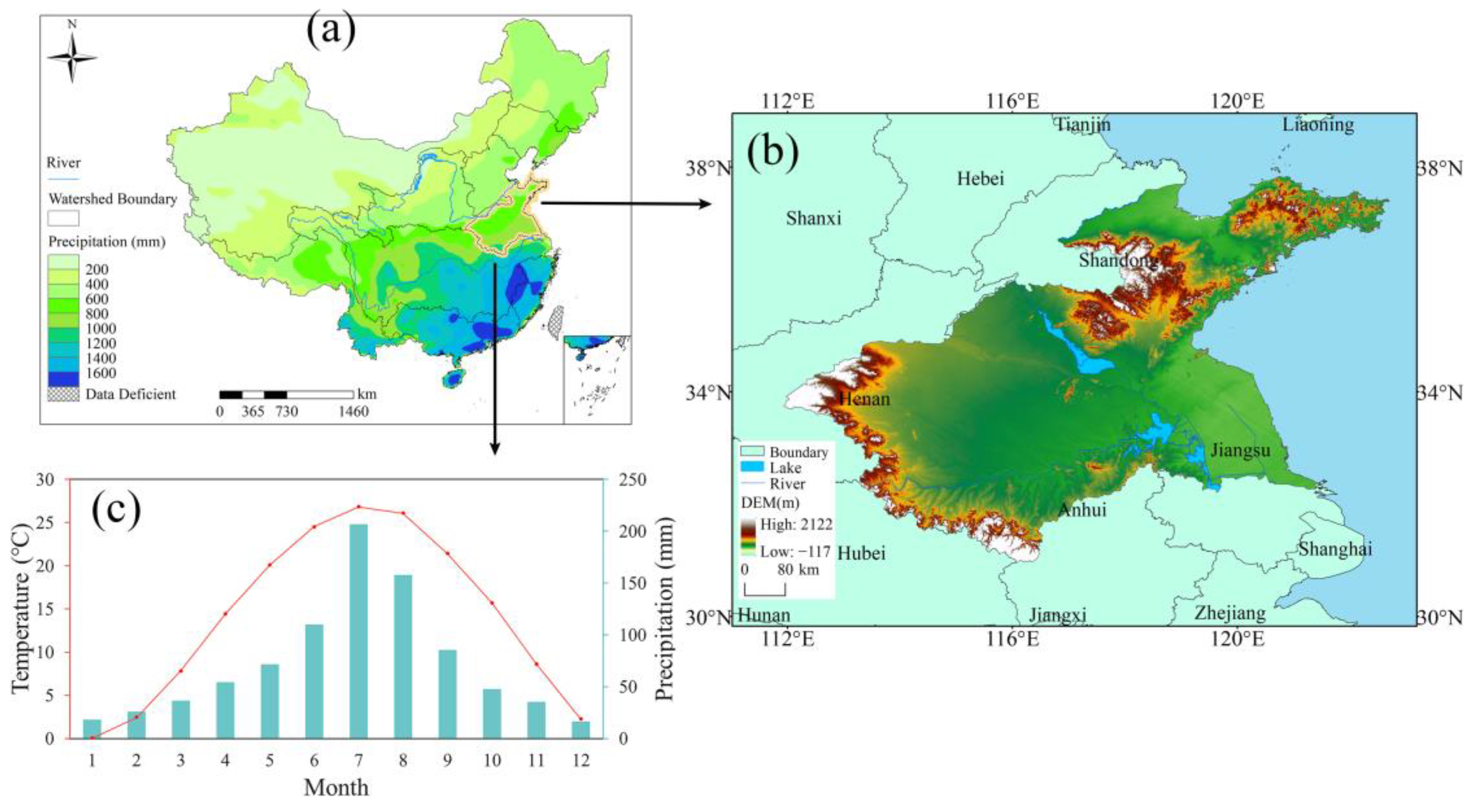
Figure 1. Relevant information on the study area. (a) Spatial distribution of annual mean precipitation over China from 1961 to 2020. (b) Overview of the study area. (c) Monthly variations in average temperature and precipitation over the Huai River Basin from 1961 to 2020. The vector map of boundaries of China’s ten major river basins used in (a) is sourced from the China Institute of Water Resource and Hydropower Research.
Atmosphere 14 01497 g001
Figure 2. The spatial distribution of the climatological average of various extreme precipitation indices over the HRB from 1961 to 2020. The indices are (a) CDD, (b) CWD, (c) R10mm, (d) PRCPTOT, (e) SDII, (f) Rx1day, (g) Rx5day, and (h) R95p.
Atmosphere 14 01497 g002
Figure 3. The spatial distribution of trends over the HRB from 1961 to 2020 for CDD (a), CWD (b), R10mm (c), PRCPTOT (d), SDII (e), Rx1day (f), Rx5day (g), R95p (h). Cross-hatch regions represent areas with statistically significant trends at a 95% confidence level.
Atmosphere 14 01497 g003
Figure 4. Taylor diagram for the 35 models of NEX-GDDP-CMIP6 simulating trends in spatial change in extreme precipitation indices over the HRB from 1995 to 2014. (a) CDD, (b) CWD, (c) R10mm, (d) PRCPTOT, (e) SDII, (f) Rx1day, (g) Rx5day, (h) R95p.
Atmosphere 14 01497 g004
Figure 5. Ranking of the simulation capability of 35 models of NEX-GDDP-CMIP6 on the trend of extreme precipitation over the HRB from 1995 to 2014. The numbers in the figure represent the ranking of each climate model in terms of simulation capabilities for different extreme precipitation indices.
Atmosphere 14 01497 g005
Figure 6. Taylor diagram for the 35 models of NEX-GDDP-CMIP6 simulating climatology in extreme precipitation indices over the HRB from 1995 to 2014. (a) CDD, (b) CWD, (c) R10mm, (d) PRCPTOT, (e) SDII, (f) Rx1day, (g) Rx5day, (h) R95p.
Atmosphere 14 01497 g006
Figure 7. Ranking of the simulation capability of 35 models of NEX-GDDP-CMIP6 on the climatological mean states of extreme precipitation over the HRB from 1995 to 2014. The numbers in the figure represent the ranking of each climate model in terms of simulation capabilities for different extreme precipitation indices.
Atmosphere 14 01497 g007
Figure 8. Ranking of the simulation capability of 35 models of NEX-GDDP-CMIP6 on the climate and trend of extreme precipitation based on frequency index (CDD, CWD, R10mm) and intensity index (PRCPTOT, SDII, Rx1day, Rx5day, R95p) over the HRB from 1995 to 2014. The numbers in the figure represent the ranking of each climate model in terms of simulation capabilities for different extreme precipitation indices.
Atmosphere 14 01497 g008
Figure 9. Comparison of the spatial distribution of average annual precipitation (a,b) between the observed (a) and preferred (b) models’ ensemble and spatial pattern of their bias (c) over the HRB from 1995 to 2014.
Atmosphere 14 01497 g009
Figure 10. Comparison of the spatial distribution of climatological means between the observed (columns 1 and 3) and preferred models’ ensemble (columns 2 and 4) for CDD (a), CWD (b), R10mm (c), PRCPTOT (d), SDII (e), Rx1day (f), Rx5day (g), R95p (h).
Atmosphere 14 01497 g010
Figure 11. Comparison of the spatial distribution of trends between the observed (columns 1 and 3) and preferred models’ ensemble (columns 2 and 4) for CDD (a), CWD (b), R10mm (c), PRCPTOT (d), SDII (e), Rx1day (f), Rx5day (g), R95p (h). Cross-hatch regions represent areas with statistically significant trends at a 95% confidence level.
Atmosphere 14 01497 g011
Figure 12. Taylor diagram for the preferred models’ simulation of climatological means in extreme precipitation indices over the HRB from 1995 to 2014. (a) CDD, (b) CWD, (c) R10mm, (d) PRCPTOT, (e) SDII, (f) Rx1day, (g) Rx5day, (h) R95p.
Atmosphere 14 01497 g012
Figure 13. Taylor diagram for the preferred models’ simulation of trends in spatial change in extreme precipitation indices over the HRB from 1995 to 2014. (a) CDD, (b) CWD, (c) R10mm, (d) PRCPTOT, (e) SDII, (f) Rx1day, (g) Rx5day, (h) R95p.
Atmosphere 14 01497 g013
Table 1. Information on 35 global climate models from NEX-GDDP-CMIP6.
Model NameIntuition/CountryHorizontal Resolution (lon × lat)
GridDegree
ACCESS-CM2 [44]CSIRO-ARCCSS/Australia144 × 1921.875° × 1.25°
ACCESS-ESM1-5 [45]CSIRO/Australia192 × 1451.875° × 1.25°
BCC-CSM2-MR [46]BCC/China160 × 3201.125° × 1.125°
CanESM5 [47]CCCma/Canada64 × 1282.812° × 2.77°
CESM2 [48]NCAR/USA288 × 1921.25° × 0.94°
CESM2-WACCM [49]NCAR/USA288 × 1921.25° × 0.94°
CMCC-CM2-SR5 [50]CMCC/Italy288 × 1921.25° × 0.9375°
CMCC-ESM2 [51]CMCC/Italy288 × 1921.25° × 0.94°
CNRM-CM6-1 [52]CNRM-CERFACS/France64 × 1281.406° × 1.406°
CNRM-ESM2-1 [53]CNRM-CERFACS/France128 × 2561.406° × 1.406°
EC-Earth3 [54]EC-Earth-Consortium/EC-Earth consortium256 × 5120.703° × 0.703°
EC-Earth3-Veg-LR [54]EC-Earth-Consortium/EC-Earth consortium256 × 5121.125° × 1.125°
FGOALS-g3 [55]CAS/China180 × 802° × 2.025°
GFDL-CM4 [56]NOAA-GFDL/USA288 × 1801.25° × 1°
GFDL-CM4_gr2 [56]NOAA-GFDL/USA90 × 1444° × 1.25°
GFDL-ESM4 [57]NOAA-GFDL/USA288 × 1801.25° × 1°
GISS-E2-1-G [58]NASA-GISS/USA144 × 902.5° × 2°
HadGEM3-GC31-LL [59]MOHC, NERC/UK144 × 1921.875° × 1.25°
HadGEM3-GC31-MM [60]MOHC/UK324 × 432~0.8° × 0.6°
IITM-ESM [61]CCCR-IITM/India192 × 941.875° × 1.915°
INM-CM4-8 [62]INM/Russia180 × 1202° × 1.5°
INM-CM5-0 [63]INM/Russia180 × 1202° × 1.5°
IPSL-CM6A-LR [64]IPSL/France144 × 1432.5° × 1.259°
KACE-1-0-G [65]NIMS-KMA/Republic of Korea144 × 1921.875° × 1.25°
KIOST-ESM [65]KIOST/Republic of Korea96 × 1920.938° × 0.938°
MIROC6 [66]MIROC/Japan256 × 1281.403° × 1.403°
MIROC-ES2L [67]MIROC/Japan256 × 1281.403° × 1.403°
MPI-ESM1-2-HR [68]MPI-M, DWD, DKRZ/Germany384 × 1920.938° × 0.939°
MPI-ESM1-2-LR [69]MPI-M, AWI, DKRZ, DWD/Germany192 × 961.9° × 1.9°
MRI-ESM2-0 [70]MRI/Japan320 × 1601.125° × 1.125°
NESM3 [71]NUIST/China192 × 961.88° × 1.88°
NorESM2-LM [72]NCC/Norway144 × 962.5° × 1.89°
NorESM2-MM [72]NCC/Norway288 × 1921.25° × 0.94°
TaiESM1 [73]AS-RCEC/Taiwan, China288 × 1921.25° × 0.94°
UKESM1-0-LL [74]MOHC/UK144 × 1921.875° × 1.25°
Table 2. The extreme precipitation index information used in this study.
IndexDescriptive NameDefinitionUnits
Indexes for frequencyCDDConsecutive dry daysMaximum number of consecutive dry daysd
CWDConsecutive wet daysMaximum number of consecutive wet daysd
R10 mmNumber of heavy precipitation daysAnnual count of days when RR ≥ 10 mmd
Indexes for intensityPRCPTOTWet day precipitationAnnual total precipitation from wet daysmm
SDIISimple daily intensity indexAverage precipitation on wet daysmm d−1
Rx1dayMaximum 1-day precipitationMonthly maximum 1-day precipitation mm
Rx5dayMaximum consecutive 5-day precipitationMonthly maximum consecutive 5-day precipitationmm
R95pVery wet day precipitationAnnual total precipitation when RR > 95th percentile of 1961–2020 dailymm
Disclaimer/Publisher’s Note: The statements, opinions and data contained in all publications are solely those of the individual author(s) and contributor(s) and not of MDPI and/or the editor(s). MDPI and/or the editor(s) disclaim responsibility for any injury to people or property resulting from any ideas, methods, instructions or products referred to in the content.