Abstract
In this study, a rainstorm of the type experienced on 20 July 2021 over central East China was simulated using the first-generation Chinese Reanalysis datasets and Global Land Data Assimilation System datasets, and the Noah land surface model coupled with the advanced weather research and forecasting model. Based on this, the gridded planetary boundary layer (PBL) profiles and ensemble states within soil perturbations were collected to investigate the typical land–atmosphere coupling chain during this modeled rainstorm by using various local coupling metrics and introduced ensemble statistical metrics. The results show that (1) except for the stratospheric thermodynamics and the surface temperature over mountain areas, the main characteristics of the mid-low atmospheric layers and the surface have been well captured in this modeled rainstorm; (2) the typical coupling intensity is characterized by the dominant morning moistening, an early afternoon weak PBL warming factor of around 2, a noontime buoyant mixing temperature deficit around 274 K, daytime PBL and surface latent flux contributions of around 100 and 280 W/m2, respectively, and significant afternoon soil-surface latent flux coupling; and (3) an overall negative soil–rainfall relationship can be identified from the ensemble metrics in which the moist static energy is more significant than PBL height, and this is consistent with the significance of daytime surface moistening indicated by local coupling metrics. Taking the multi-process chain in chronological order, the wet soil contributes greatly to daytime moisture evaporation, which then increases the early noon PBL warming and enhances the noon period buoyant mixing within weak moist heating; however, this is suppressed by large-scale forcing such as the upper southwestern inflows of rainstorms, which further significantly shapes the spatial distribution of the statistical metrics. These quantitatively described local daytime couplings highlight the potential local application of promoting public weather forecasting efforts, while the high spatial differences in the coupling indicate the more applicable threshold diagnoses within finer-scale spatial investigations.
1. Introduction
The extreme rainfall on 20 July 2021 over central East China caused great loss for both society and individuals, and various greater-scale atmospheric systems have been found to be the possible culprits, while local surface factors are still under-explored [1,2,3,4]. In particular, the comprehensive local factors indicated by the land–atmosphere coupling in weather and climate are inherently challenging and complex [5,6]. The effect on rainfall of soil moisture (SM), one of the key factors in land–atmosphere coupling, is especially evident during both model [7] and observational [8] studies. This effect has been determined through various conventional approaches (or feedback chains) but with large uncertainties because of numerous coupling deficits [9]. Therefore, quantifying the local coupling characteristics of this severe rainstorm can be of great significance for resharpening the local typical feedback chain to promote future public service efforts in local weather forecasting.
Early studies have shown that rainfall is highly coupled with SM in many “hot spot” (or typical) regions, as indicated by the extensive data of the global observation network [10], where local morning SM can significantly affect afternoon convection [11]. However, against a background of shifted local surface caused by global warming [12], these rainfall-related couplings have been found to intersect with typical local characteristics such as the regional soil moisture gradient and soil thickness [13,14]. However, due to the immeasurable uncertainties in observational and model deficits, regional coupling characteristics can be typically varied in many model-relative regional studies, as indicated by the complex surface intersection between soil moisture, land cover, land surface model (LSM), the resolution scale of the coupling model, and so on [15,16,17,18,19,20]. Generally, local land–atmosphere coupling (LoCo) uncertainties (e.g., positive and negative couplings coexisting, as well as highly discontinuous couplings) in models and datasets have resulted in complex coupling physics and further limited the predictability of energy and water budgets at a larger scale.
To quantify the various typical LoCo characteristics, the well-known Global Energy and Water Cycle Experiment (GEWEX) has promoted observational evidence rooted in process-level scales over decades, in that the variations of surface soil moisture, evapotranspiration, PBL states, PBL top entrainment, near-surface atmospheric thermal conditions, precipitation and/or clouds resulting from surface changes have been investigated through energy budget analysis and/or state covariations to evaluate various typical surface advantages and/or deficits, e.g., morning PBL moistening or deepening [21,22], local and non-local physics resulting in PBL top humidity changes [23,24], diagnostic states regarding well-mixed turbulence [25,26,27], surface and atmospheric flux contributions under surface thermal and moisture coevolution space [28], atmospheric state responses to SM [29,30,31], the persistence of SM anomalies [32], and so on. These quite different measurements have been documented into one overall LoCo process chain, and further collected into the Coupling Metrics Toolkit (www.coupling-metrics.com, accessed on 18 September 2023), in order to foster broader participation [33].
However, physical and statistical LoCo metrics are highly distinguished on the process scales of their observational physics and/or statistics, which results in regional model and/or dataset applications favoring limited metrics with large samples for robust coupling characteristics but usually only considering semi-coupling because overall typical LoCo chains in the real world can be step-wise multi-processes [34,35,36,37]. Meanwhile, the uniformly scaled multi-metrics/-processes could be challenging because of insufficient PBL observations and/or coupling theory deficits (e.g., the varied scale dependence) [10,11,12,33]. Conversely, ensemble simulations within perturbed SM can achieve the overall relation chains (e.g., correlations) during regional studies [38,39], but are usually non-observational and qualitative (e.g., negative and/or positive). Clearly, these scale dependence deficits have resulted in the overall rainfall-related coupling chain being shown to be incomplete and/or untrue.
In general, due to the unsolved spatiotemporal scale issues of coupling theory and the expensive surface-PBL observations, the coupling indicated by the highly distinguished LoCo metrics and the relation-chain-like ensemble statistical correlations lack mutual confirmation required to sharpen the plausible overall LoCo chain during regional weather applications. In particular, the ensemble statistical correlations lack verification of their reliability. To fill this gap, this study has evaluated the LoCo characteristics of the recent extreme rainstorm that occurred over central East China on resolved model grids by using various LoCo metrics and ensemble statistical relations to highlight the perspectives that multi-process and ensemble metrics can offer on the overall LoCo chain for possible application in local weather forecasting.
2. Model and Data
This study has used the Unified Noah Land Surface Model (Noah LSM) [40] coupled with the advanced weather research and forecasting model (WRF, Version 3.9.1) [41] to conduct a land–atmosphere coupling simulation of a rainstorm of the type experienced on 20 July 2021. The Noah LSM can run on finer temporal and spatial steps, and it has been widely used in numerical weather prediction and well-verified in local coupling studies [28,34,35,36,37].
As seen in Figure 1, two domains (D01 and D02) are one-way nested and centered at 113.45° E, 33.85° N with 51 model levels topped at 50 hPa and run within a 60 s time step. The outer and inner domain resolutions are 12 and 4 Km with 100 × 100 and 165 × 159 grids, respectively. During both domains, the microphysics adopt the Thompson scheme [42], the short- and long-wave physics adopt the RRTMG schemes [43], the cumulus parameterization physics adopt the Kain–Fritsch scheme [44], and the surface-layer physics adopt the Revised MM5 scheme [45]. The Yonsei University PBL scheme (YSU) uses a non-local entrainment treatment method more suitable for nocturnal PBL within lower heights [46]. For this reason, 21 levels below 1 Km are created to achieve finer PBL profiles using YSU physics.
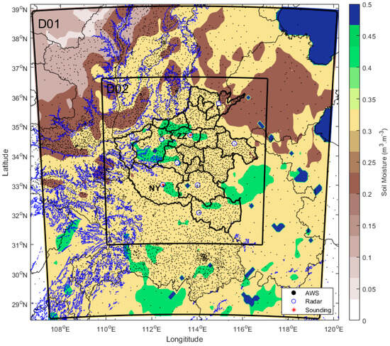
Figure 1.
Regions and observations. Topography higher than 500 m (blue contours), GLDAS surface soil moisture (shaded) at 00:00 on 20 July, locations of AWS observations (black solid points), soundings (red asterisks), radars (blue circles), and model domains (black boxes).
The atmospheric forcing datasets are collected from the first-generation global atmospheric/land-surface reanalysis project (CRA40), which has a resolution of 34 Km, 64 pressure levels, and 6 and 3 h intervals for atmospheric and surface layers, respectively [47,48]. Meanwhile, the Noah LSM driven by the Global Land Data Assimilation System reanalysis (GLDAS) has a resolution of 0.25°, 3 h intervals, and 4 layers [49]. In addition, the 3 s terrain data derived from the United States Geological Survey (USGS) and the 15 s land cover data derived from the Moderate-resolution Imaging Spectroradiometer (MODIS) product have been taken as the static underlying datasets.
The observations used in this study mainly consist of the automatic weather stations (AWS), nine S-band Doppler weather radars, and two soundings (Figure 1) derived from the CMA Henan Meteorological Bureau. The AWS has a resolution of around 0.1° and 1 h intervals and each radar plot has a resolution of around 250 m, 11 elevation numbers, and 6 min intervals. The sounding sites Zhengzhou (ZZ) and Nanyang (NY) are taken as the two typical points of this domain to investigate the rainstorm-affected typical factors and non-typical factors, respectively. Also, the grid precipitation product of the Land Surface Data Assimilation System (CLDAS) of the CMA, which has a resolution of 0.1° × 0.1° and 1 h intervals [50] during the local operational application, is collected to fulfill the accumulative rainfall validation. It should also be noted that the local hourly CLDAS rainfall products are used for calculating the longer time series accumulated precipitation (e.g., 12 h rainfall) in order to avoid discontinuities in AWS observations at different times. The AWS datasets are also supplied to ensure the objectivity of instantaneous observations.
3. Experiments
The flowchart of this study is shown in Figure 2. Firstly, all the datasets used for various coupling metric calculations are prepared as described in the following sections. The simulation derived from the CMA datasets is compared with various local observations to ensure one basis of this study, which is that the main land–atmosphere state characteristics have been well documented in this modeled rainstorm (See Section 5.1), based on which, the ensemble forecast within perturbated soil moisture is conducted to achieve another basis of this study, which is that reliable soil ensemble forecasts are obtained. Secondly, the gridded land-PBL profiles derived from the well-modeled rainstorm and the ensemble states within soil perturbations derived from the soil ensemble forecast are collected for the calculation of LoCo metrics and ensemble statistical relations to achieve the LoCo diagnoses and the paired state relations, respectively. Finally, the above-mentioned statistics are analyzed for their main spatial and temporal characteristics to achieve the overall quantitative coupling insights during this event.
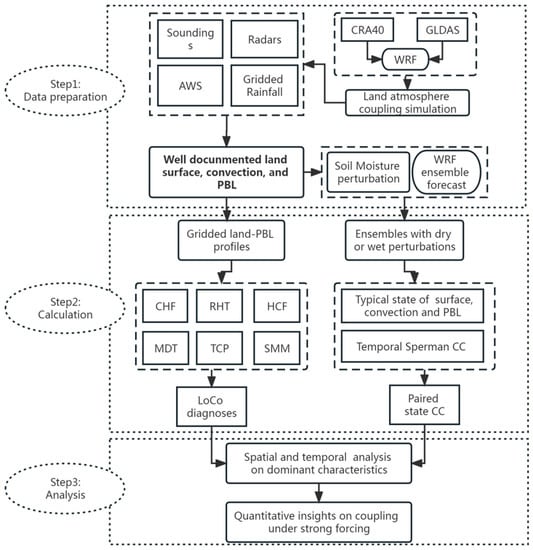
Figure 2.
Flowchart of this study. CC = correlated coefficients.
Additionally, the simulation period runs from 00:00 to 24:00 on 20 July (UTC), which includes the extreme rainfall event of ZZ city around late afternoon on 20 July. The inner domain (Figure 1; D02) is taken as the target region for the land–atmosphere coupling investigation. Three dry (wet) members assembled by systematically reduced (added) soil moisture at an interval amplitude with the self magnitude of 30% for the target region are conducted to generate a soil ensemble forecast [39]. In addition, the land atmospheric coupling chains indicated by various metrics have been compared to investigate the applicability of the main coupling characteristics to local weather forecasts.
It should be noted that the intermediately linked responses of the surface and the PBL to SM follow a nonlinear process relating to their distinct states of matter (e.g., water vapor, clouds, and rainfall) and physical characteristics (e.g., temperature, energy, and depth). In particular, the overall LoCo chain [33] proceeds step-wise and is typically based on process discrimination. Therefore, the simulated PBL thermal profiles (including temperature, water vapor, surface fluxes, and so on) are collected to evaluate the physically observable surface–PBL chain, while the simulated surface fluxes and SM are conducted to evaluate the statistically observable SM–surface chain. Furthermore, to comprehensively investigate the reliability of the coupling indicated by various ensemble statistics during this overall LoCo chain, the various surface–PBL states including the surface flux slope (the dominated surface fluxes), the near-surface atmospheric temperature and moisture, the model bottom and PBL average temperature and moisture, the PBL height and the moist static energy around 500 m (where the most unstable air parcel exists), and so on, are collected to evaluate their typical relationships in terms of the overall LoCo chain.
4. Methods
4.1. The Local Coupling Metrics
Table 1 shows various LoCo diagnoses derived from the Coupling Metrics Toolkits. The various surface advantages or deficits for potential convection indicated by CHF are classified by the observation-based thresholds suggested by the initial study (described in Section 5.2.1) [21,22]. The various deficits and advantages indicated by RHT [23,24], HCF [25,26,27], and MDT [28] are measured in hourly intervals. Meanwhile, we take four 6 h ranged periods to conduct both the TCP [29,30,31] and SMM [32], the diagnoses of which have been calculated from two adjacent 3 h forecasts during one period. Both sensible and latent heat fluxes for TCP (e.g., TCPSH and TCPLH) are considered, and the threshold for memory loss in SMM is set to (about 0.5). It should be noted that we set the interval simulation for the whole of 20 July 2021 to 3 h in order to assemble the necessary samples for calculating the LoCo diagnoses, and further analyses of both local daytime (00:00~12:00) and nighttime (12:00~24:00) are conducted.

Table 1.
Description of the LoCo metrics.
The typical LoCo chains can be completed by using predefined variations within temporally and/or spatially issued diagnoses to hopefully address their closure [33]. It should be noted that variations resulting from the surface (see Table 1) have been implicitly defined as the spatial difference of an instantaneous moment (e.g., surface–upper layer height differences in CHF or HCF), or both temporal and spatial differences (e.g., MDT, RHT, TCP, and SMM). In particular, the variation of the surface has been defined in the form of time lags in the cases of TCP and SMM.
4.2. The Ensemble Statistical Metrics
This study conducts ensemble forecasts with dry or wet perturbations (DP or WP) by utilizing the initially increased or decreased soil moisture () of one well-documented land–atmosphere simulation (or control run; ). The differences between DP (WP) and the control run are defined as () variations that arise from . Then, the temporal correlations () between various () variations are analyzed to identify ensemble statistical relations. The formulas for dry and wet variations are calculated as follows.
In Equations (1) and (2), and represent the ensemble members and total number (), respectively, and are the averaged state at one specific layer during the study area for the dry and wet states ( and ), respectively, and represents the control state (e.g., the well-documented modeled rainstorm). It should be noted that the state average is usually desired to remove the unrealistic land–atmosphere response present at the beginning [39].
Additionally, the strength of the relationship based on the Spearman rank correlation [51] between the averaged states ( or ) or variations ( or ) of different layers are calculated as follows.
In Equation (3), represents the index of the overall time steps , and represent two sorted states, such as PBL thermal or energy variables, and the superscript horizontal line represents the temporal average. Therefore, the coupling intensity () is identified when the value of is larger than 0.5 or less than −0.5, and its reliability is indicated by the significant level (p) when p is less than a threshold (e.g., 0.05).
In addition, to achieve the main spatial characteristics of the gridded surface–PBL profiles, LoCo diagnoses and of ensemble statistics, and these three kinds of samples (the number of which is equal to the D02 domain gird number calculated as 165 × 159) have been resampled into 100 bins and then fitted by a 2-peak Gaussian function in order to generate at most two main signals on the model grid resolved couplings. The Gaussian function is defined as , where s is the sample, a is the amplitude, b is the centroid (location), c is related to the peak width, and n is the number of peaks to fit (n = 2).
5. Results
5.1. Simulation Overview
5.1.1. Synoptic and Thermodynamics
As seen in Figure 3, for the 500 hPa level, a cyclonic Low (L) system crosses the whole central domain surrounded by three High (H) centers, while an intense Warm (W; around −4 °C) center is located to the west of the L (Figure 3a). For the 700 hPa level, the L center accompanied by an intense Cold (C; around 9 °C) center and strong easterly flows on its north edge is still holding but has clearly shrunk (Figure 3b). For the 850 hPa level, the L center accompanied by strong northeast flows on its north edge is still holding but has further shrunk (Figure 3c). For the surface level, the L center accompanied by an intense C center on its northern edge is similar to the upper-level patterns (Figure 3d). Clearly, the deep Low system holding for all levels is the primary synoptic pattern, and its range has shrunk at lower altitudes, and this is especially pronounced between the 500 and 700 hPa levels when the surrounding flows have clearly changed. This indicates a strong warm pool at the 500 hPa level but a strong cold invading below it. In addition, this Low over the relatively moist and quite warm surface (>25 °C) has lasted more than 12 h (ending at 12:00 or later); this should be attributed to the upper systems easterly developing easterly (e.g., the South Asia High) above the 300 hPa level (not shown).
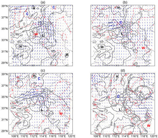
Figure 3.
Synoptic overview at 00:00 on 20 July. (a–c) The geopotential height (black lines; units: gpm), temperature (red dashed lines; units: °C), and winds (blue vectors; units: m/s) for the 500, 700, and 850 hPa levels, respectively. (d) The sea level pressure (black lines; units: hPa), temperature (red dashed lines; units: °C), and winds (blue vectors; units: m/s) for the surface layer. H = High, L = Low, C = Cold, W = Warm.
As seen in Figure 4, at 00:00 for the ZZ site, in the case of the observations, a saturated atmosphere where the difference between temperature and dew point (T-Td) is almost zero can be observed below 400 hPa, while the simulated saturated top extends up to 200 hPa, and the wind rotates counterclockwise as the pressure decreases above 850 hPa for both the observations and the simulation (Figure 4a). At 12:00 for the ZZ site, the top of the observed saturated atmosphere in the observations extends to near 300 hPa, while the simulated saturated top is now at 400 hPa, and counterclockwise rotated winds between 850 and 500 hPa can be observed in both the observations and the simulation (Figure 4b). Clearly, for the ZZ site, below 400 hPa, the regional thermodynamic conditions of this event have been well simulated, and the pressure and temperature of lifting condensation level for both the simulation (sPlcl and sTlcl) and the observations (oPlcl and oTlcl) are almost equitable. However, above 400 hPa for the ZZ site, the higher saturation top at 00:00 and lower saturation top at 12:00 of the simulation have resulted in lower and higher convective available potential energy (Cape), respectively, compared to the observations. Furthermore, at 00:00 for the NY site, below about 400 hPa, both the observed and simulated temperature and dew point profiles have behaved consistently, where counterclockwise rotated winds also can be observed, while above 400 hPa, the saturated atmosphere of the simulation is different from the dry atmosphere seen in the observations (Figure 4c). At 12:00 for the NY site, both the observed and simulated temperature profiles behaved consistently, and a shaking dew point profile of the observations can be observed when compared to the simulation, while a slightly moister atmosphere above 400 hPa in the simulation can be observed compared to the observations. Also, counterclockwise rotated winds can be observed between the surface and 500 hPa layers in both the observations and simulation (Figure 4d). The Plcl and Tlcl for both the observations and the simulation are almost equatable, while the Cape differences between the simulation and the observations for the NY site behave opposite to those of the ZZ site.
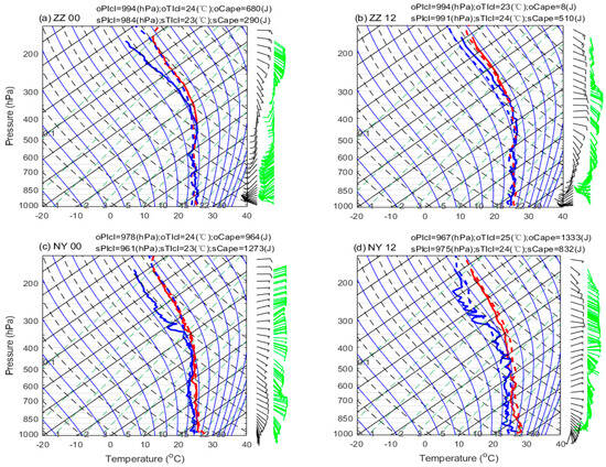
Figure 4.
Observed and simulated soundings. (a,b) The T−logP plots at 00:00 and 12:00, respectively, on 20 July for the ZZ site. In (a,b), the thick solid and thick dashed lines represent the observations and simulations, respectively, the thick red and thick blue lines represent temperature (units: °C) and dew point (units: °C), respectively, and the green and black wind barbs on the right hand represent the observed and simulated wind profiles, respectively. The isotherms (black lines), dry adiabats (dashed black lines), saturation mixing ratio (green dashed lines), moist adiabats (blue lines) are also shown. (c,d) are the same as (a,b), but for the NY site.
Obviously, the mid-low layer (below 400 hPa) thermodynamic situations of both two sites have been well simulated, and the moist atmosphere holds from 00:00 to 12:00, whereby the lifting condensation level (LCL) can be easily reached. The inverse wind directions indicate a large-scale cold front invading, and it covers almost all layers at 00:00 and then shrinks to the mid-low layers at 12:00 for the ZZ site, while it has decreased from the mid-low layers at 00:00 to the low layers at 12:00 for the NY site. In contrast, the observed upper southern flows have increased from 00:00 to 12:00 for both two sites. This indicates a northerly moving warm front. However, the simulation has a clear large bias on the upper-level (above 400 hPa) systems, and this is especially pronounced for the NY site at 00:00, which indicates possible dataset deficits (e.g., sounding drifts).
5.1.2. Convection and Rainfall
The observed composite reflectivity (CR) and 3 h accumulative rainfall () are compared with the simulation to validate the modeled performance of convection (defined as when CR > 10 dBZ) and rainfall. The diurnally observed convection is relatively stronger (>26 dBZ) compared to the simulation (>24 dBZ), and this difference is especially pronounced at the beginning of the period (e.g., from 03:00 to 06:00) (Figure 5a). And the dominant convection in the observations is also stronger (around 28 dBZ), but with a lower frequency of around 2000, which is almost half that of the simulation (Figure 5b). The varied between 0.3 and 0.5 on 20 July, with the most pronounced at 12:00 (when the extreme rainfall ends) reaching nearly 0.6. Meanwhile, RMSE shows the opposite behavior to . In particular, a significant decrease (from 17 to 13 dBZ) at the beginning of the period and a significant increase (from 13 to 16 dBZ) at the end can be seen (Figure 5c). The significantly high and low RMSE (when > 0.3 and RMSE < 14 dBZ) indicate that the main convection can be well captured from local noon to early evening (06:00~15:00), but before and following that, the simulated likely misses the true convection pattern. Additionally, the daytime shows significantly negative values over the main rainfall area (Figure 5d), and this is consistent with the opposite variation trend of the domain-averaged CR during the daytime (Figure 5a).
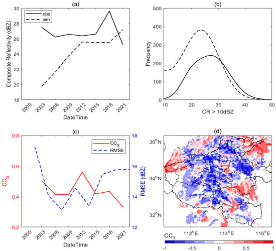
Figure 5.
Simulated and observed convection comparison. (a) The domain-averaged 3 h interval composite reflectivity (CR) against time. (b) The frequency of the 3 h interval CR that exceeds 10 dBZ averaged over the whole simulation period. (c) The spatially correlated coefficients () and root mean square errors (RMSE) of CR over the simulated period. (d) The temporally correlated coefficients () of CR over the daytime period (00:00~12:00) on 20 July 2021.
The domain-averaged 3 h rainfall () of the simulation shows a significant increase from local noon to early night, which is consistent with observations, but with lower values (Figure 6a). Nevertheless, significant rainfall biases can be found at the beginning and ending periods. Meanwhile, the frequency of the is larger in the simulation, which is especially pronounced for light rainfall (e.g., < 20 mm), though the frequency distributions of both the simulation and the observations behaved consistently (when is larger than 10 mm) (Figure 6b). Additionally, the daytime rainfall amount has a of about 0.62, and the shapes of the heavy rainfall areas are especially similar (Figure 6c,d). Also, the rainfall extremes (>200 mm) are both located at the ZZ city site. This indicates that the main rainfall spatial characteristics and location of extremes have been well simulated. However, the northeastern edge of this developing rainfall in the simulation has been clearly missed compared to the observations. This is consistent with the biased convection that developed in the north (Figure 5c,d) and the biased thermodynamics within southern flows in the upper layers (Figure 4b,d).
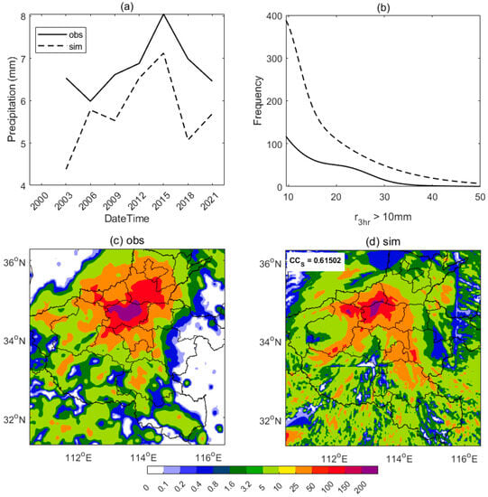
Figure 6.
Simulated and observed rainfall comparison. (a) The domain-averaged 3 h rainfall against time. (b) The frequency distribution of the 3 h rainfall () that exceeds 10 mm averaged over the whole simulation period. (c,d) The 12 h accumulated precipitation (shaded, units: mm) during the daytime (00:00~12:00) on 20 July for CLDAS observations and the simulation, respectively; the spatial correlation coefficient () is also shown.
Overall, though the modeled convection and rainfall are relatively weaker than those in the observations, both the main convection and rainfall characteristics have been well captured from local noon to early evening when the main rainstorm occurs. However, the biased convection and rainfall during later periods consistent with the biased upper systems show the potential deficits in the model calculation (e.g., the unsolved nonlinear physics), while the biases in the initial periods can be attributed to unbalanced model states (e.g., the unsolved model spin up or insufficient datasets).
5.1.3. Underlying Surface Characteristics
The domain-averaged simulation shows a similar diurnal variation to the observations but is warmer than the latter, an effect that is especially pronounced around the local noon (Figure 7a). However, the frequency of the temporally averaged in the observations is mostly above that of the simulation (Figure 7b). Clearly, the warmer diurnal variation and colder frequency spatial distribution indicate the overall simulated characteristics have fallen into two different phases. However, the observed frequency is below that of the simulation at around 302 K, in which the frequency is around 5000, which is almost twice the former. Additionally, the shows a significant decrease at the beginning, then a relatively flat variation of around 0.2 from local morning to late afternoon, and a significant decrease at the end (Figure 7c). Meanwhile, RMSE shows an opposite variation to , and the significant RMSE of around 8 K occurs at local noontime. Furthermore, a daytime that exceeds 0.5 with confidence (whose significance level is lower than 0.05) can be observed in most areas, while significant negative relations can be observed over the Southern Taihang mountain (Figure 7d). Clearly, the significantly negatively biased daytime surface temperature over mountain areas has mainly contributed to the phase differential surface characteristics.
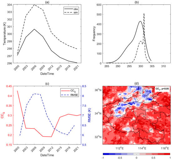
Figure 7.
Simulated and observed surface comparison. (a) The domain−averaged 3 h surface temperature against time. (b) The frequency distribution of the 3 h surface temperature averaged over the whole simulation period. (c) The spatially correlated coefficients () and root mean square errors (RMSE) of the surface temperature over the simulated period. (d) The temporally correlated coefficients () of the surface temperature during the daytime on 20 July 2021; a significance level of less than 0.05 (p < 0.05; dotted) is also shown.
In general, the long-lasting Low system with an upper warm flow and a lower strong cold front, the mid-low layer thermodynamic situations, the convection and rainfall spatiotemporal characteristics, and the diurnal surface thermal characteristics are consistent with the available observations. However, the stratospheric (higher than 400 hPa) thermodynamics consistent with the northernly developed rainfall and convection, and the temperature over mountain areas have been found to be biased. Except for in the case of the mountain areas, the main characteristics of the low atmospheric layers and the surface have been well captured by the model; therefore, this is taken as the basis of the surface–atmosphere state for further investigation.
5.2. The Local Coupling Evaluation
5.2.1. CHF
The thresholds of CHF for typical discriminating characteristics are defined as follows. For atmospherically controlled advantage (ACA), TCP varies between 0 and 300 (J/Kg) and HIlow varies between 0 and 5 (°C). For wet soil advantage (WSA), TCP varies between 0 and 230 (J/Kg) and HIlow varies between 5 and 10 (°C). For dry soil advantage (DSA), TCP varies between 180 and 300 (J/Kg) and HIlow varies between 10 and 15 (°C). For the trans region (TR), TCP varies between 100 and 180 (J/Kg) and HIlow varies between 10 and 15 (°C). For stable regions when it is too dry for rainfall (SRD), HIlow is larger than 15 (°C), and for regions when the atmosphere is too stable for rainfall (SRC), CTP is smaller than 0 (J/Kg).
At 00:00 on 20 July (local morning time), most grid points have fallen into the ACA and WSA regions during the CHF, while fewer grid points have fallen into the TR, DSA, and SRC regions (Figure 8a). In particular, one SRC region lies in the northwest domain, which is near the center of the upper Low system (Figure 3a,b), the adjacent TR and DSA areas are located on the northwest corner of the D02 domain, two WSA areas are located in the northeast corner and southeast of the D02 domain, respectively, and most of the D02 domain is occupied by ACA (Figure 8b).
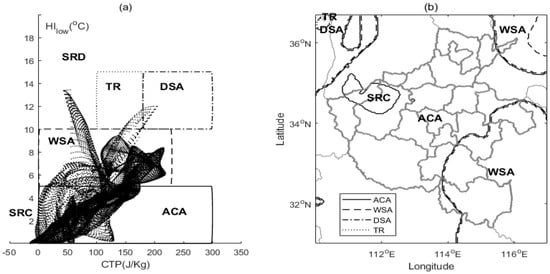
Figure 8.
The conventional trigger potential analysis at 00:00 on 20 July. (a) The scatter plots for all grids in CHF describing atmospheric controls on soil moisture–rainfall feedback. (b) The representative regions within the D02 domain, based on CHF scatter plots for all grids. In (a,b), ACA, WSA, DSA, and TR regions are denoted by solid, dashed, dash-dotted, and dotted lines, respectively. ACA = atmospherically controlled advantage, WSA = wet soil advantage, DSA = dry soil advantage, TR = trans region, SRC = stable region when atmospherically controlled, and SRD = stable region when it is too dry for rainfall.
Moreover, the consistent distributions between ACA and the strong forcing (Figure 3), and between the northwestern-southwestern diagonal line of the DSA-WSA distributions and the initial SM gradient (Figure 1), likely indicate that the easily triggered rainfall controlled by the atmosphere and the backslash-like diagonally negative-positive feedback controlled by the surface are robust to some extent. However, the distributions of these potentials are quite different from other regional studies such as over the United States [22] and Tibet [37], which should be due to differences in the local surface and upper atmosphere between these regions.
In addition, the CTP values of SRC are mostly negative, and the HIlow values of SR are quite small; this indicates that the atmosphere is likely too stable for rain to occur near the storm center. Meanwhile, the moderate CTP and high HIlow values of the TR area indicate a neutral boundary layer and dry surface, and additional CTP is needed to meet with convection in the northwest region. Clearly, except in the cases of SRC and TR, regions are favorable for potential convection as indicated by ACA, WSA, and DSA. Generally, the backslash-like negative-positive feedback and atmospheric suppression have dominated the morning convection trigger potentials.
5.2.2. RHT
The relative humidity tendency (RHT) describes the RH tendency of the PBL top that results from surface evaporation (SE), boundary layer growth (BLG), boundary layer warming (BLW), and dry air entrainment (DE). Non-evaporation (NE) has also been included for broader factor investigation. These are point-wise indicators for local cloud development [23,24]. Therefore, the main characteristics of RHT have been analyzed using temporally averaged diagnoses.
The PBL height of the ZZ site varies consistently with RH at the PBL top, and a significant decrease and increase during the beginning and ending periods, respectively, can be observed (Figure 9a). In particular, the PBL height decreases to nearly 0 at local noontime while RH at the PBL top is mostly larger than 0.8. However, the PBL height of the NY site shows opposite behavior in terms of the RH at the PBL top, and a significant daytime increase in PBL height but a decrease in RH can be observed, with the reverse occurring at night (Figure 9b). In particular, the growing PBL height and decreasing RH reach maxima of around 1000 m and 0.65, respectively, at local noon, while a significant PBL top moistening at lower PBL occurs in the late afternoon. Additionally, in the case of the ZZ site, a significant RHT tendency at the local early noon period with positive BLW, EF, and BLG can be observed (Figure 9c). While, in the case of the NY site, a positive RHT can be observed in the afternoon in addition to in the early noon period (Figure 9d). In particular, EF increases at early night for both the ZZ and NY sites, while the intermittent RHT, BLG, BLW, and absent DE for both the ZZ and NY sites indicate that the diurnal PBL clouds that develop due to local surface effects are highly nonlinear.
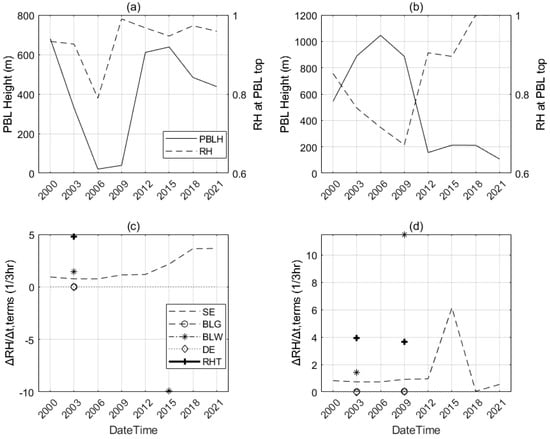
Figure 9.
The relative humidity tendency framework. Daily evolution of the boundary layer height and relative humidity at the boundary layer top for (a) the ZZ site and (b) the NY site, respectively. And the four relative humidity tendency terms, surface evaporation (SE, dashed line; unit: 1), boundary layer growth (BLG, circle; unit: %/3 h), boundary layer warming (BLW, asterisk; unit: %/3 h), dry air entrainment (DE, diamond; unit: %/3 h), and the total relative humidity tendency (RHT, cross; unit: %/3 h) for (c) the ZZ site and (d) the NY site, respectively.
RHT is mostly distributed around 4.0 with a significant frequency of around 3000 (Figure 10a,b). SE is mostly distributed around 0.85 with a significant frequency of around 1500. NE is mostly distributed around 1.9 with a significant frequency of around 600. DE is narrowly distributed around 0 with a significant frequency of around 1500. BLW is especially broadly distributed around 1.9 with a significant frequency of around 500. Nevertheless, BLG is narrowly distributed around 0.02 with a significant frequency of around 800. Clearly, SE and BLW are the largest contributors to RHT, while NE has shown relative significance during this event. Additionally, the spatial distribution of NE has behaved consistently with BLW, and strong SE surrounding the main rainfall area, weaker BLG, and weak (mostly negative) DE can be identified. It is obvious that except for the main rainfall area, EF and BLW have played the dominant roles in local PBL cloud development, while the consistent BLW and NE distribution also indicates the significant environmental factors except for the SE that directly account for the surface factors.
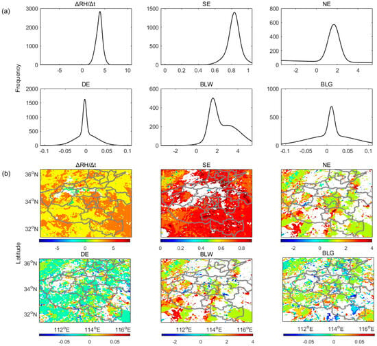
Figure 10.
(a) Frequency distribution of spatially averaged RHT terms and the non-evaporative term (NE) during the daytime on 20 July 2021. (b) The spatial distribution of temporally averaged terms.
The equitable RHT dominated by BLW and SE at early noontime when the RH begins to decrease for both the ZZ and NY sites indicates that the early noon surface–PBL coupling is characterized by the surface moistening but PBL clouds reducing. Meanwhile, the overall daytime PBL clouds resulting from the surface effects are generally dominated by BLW and SE, while the consistent distribution between diminished BLG and strong NE indicates the significantly indirect role of SE, which weakens the development of PBL clouds (e.g., through reducing, in order, surface heating, BLG, and DE). The strong surface moistening of the early noon period with overall weak dry air aloft is consistent with the description of Ek’s theory [24]. However, the different relative contributions of different RHT terms compared to those seen in Ek’s cases [23] should be attributed to the uniquely varied local characteristics during this rainstorm. Nevertheless, the opposite diurnal variations of PBL height and the quite discontinuous RHT indicate the highly nonlinear coupling resulting from varied surfaces.
5.2.3. HCF
for the ZZ site shows a sharp increase at the start of the period accompanied by increasing , weakened rainfall, and developing clouds (Figure 11a). In particular, has met with at local noontime, followed by the heavily developed rainfall and clouds accompanied by sharply decreased and during the afternoon. Nevertheless, and rainfall slowly decrease during the night, while sharply increases early in the night, but decreases to meet with late at night, when rainfall and clouds developed. Meanwhile, for the NY site shows a similar diurnal variation to the ZZ site but with a time lag of around 3 h, while, shows a similar daytime variation to the ZZ site but runs 3 h ahead at night (Figure 11b). Furthermore, the difference between and (or ) and the developing QClouds during the day predict the following rainfall for both the ZZ and NY sites. Additionally, for the domain-averaged variation, has met with and at around local noon. In particular, shows a bimodal phase, which is pronounced around local early noon and late afternoon, respectively (Figure 11c). In addition, shows a pronounced decrease during the daytime, while shows an increase at the start of the period (it lies at around 500 m) and a decrease during the afternoon (Figure 11d). Nevertheless, is significant around 09:00 when the extreme event occurs, while is especially pronounced in the afternoon.
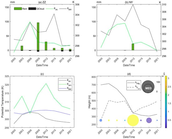
Figure 11.
The heat condensation framework. (a,b) A comparison between the buoyant mixing potential temperature (, black line; units: K) and 2 m temperature (, green line; units: K) during the whole simulation period for the ZZ and NY sites, respectively. Precipitation (green bars; units: mm) is binned by 3 hr accumulations, black bars represent the cloud water (QCloud; units: 0.1 g/Kg). (c) The domain-averaged HCF diagnoses such as , , and , against time. (d) Domain-averaged HCF diagnoses such as , , (bubble shaded) and (bubble size), against time.
The distribution is pronounced at around 1000 m with a frequency of around 1100 (Figure 12a). And shows an inverted L-shaped distribution, which is pronounced and has a maximum frequency at a value of around 90. Meanwhile, the distribution is narrowly centered at around 274 K with a frequency of around 2800. Clearly, the L-shaped frequency distribution indicates that the chances of are significantly high or low, and the most frequent is quite small (e.g., about 1 K larger than zero degrees Celsius). Additionally, except in the northwest region where the upper low-value system lasts, its surrounding is mostly around 1000 m (Figure 12b). The high lies on the east while the low is on the west, and there are three null regions during the high region. Nevertheless, except for the marginal areas, low can be observed in most areas.
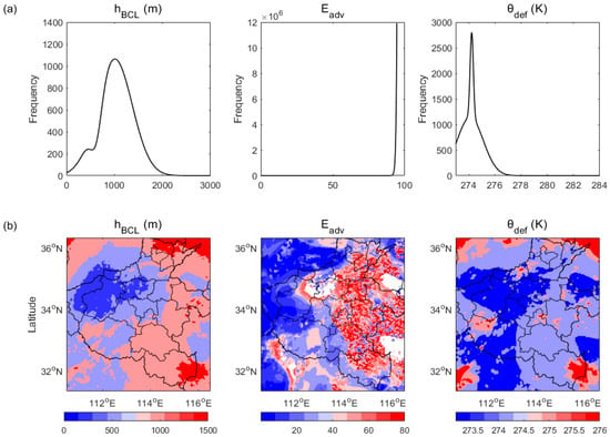
Figure 12.
(a) Frequency distribution of mean HCF diagnoses such as , and during local daytime on 20 July 2021. (b) is the same as (a) but showing the spatial distribution of temporally averaged diagnoses over local daytime.
The overall , , and intersection indicates the quite pronounced advantage of triggering local convection for the whole domain at local noon. In particular, lower (or ) within developing clouds could favor subsequent rainfall. Meanwhile, the overall and intersection where maximum occurs shows the significant latent flux advantages with saturation deficits of the PBL top after the extreme event. In contrast, the small with a relatively larger from 03:00 to 06:00 shows the overall pronounced moist energy advantages within at around 500 m. These low buoyant mixing deficits with barely null separation for reaching the transition height and favorable latent flux advantages within lower transition height show that the overall convection initiation is significantly local and likely moist, and this is consistent with the cloudy case of a previous study [27]. Moreover, the boundary condensation layer height of 1000 m and lower temperature deficit of around 274 K, and significant moistening advantages have dominated the local convection and rainfall during the daytime. However, the lower , and on the west but higher , and on the east indicate the clear regional differences between local coupling characteristics. Spatial differences between these findings and those of previous studies [25,27] should be attributed to the unsolved nonlinear physics in surface–PBL feedback.
5.2.4. MDT
During local daytime, , , and for the ZZ and NY sites are 3.3 W/m2, 63.4 W/m2, and 0.05, and 56.06 W/m2, 252.1 W/m2, and 0.22, respectively. Meanwhile, , , and for the ZZ and NY sites are 47.84 W/m2, 53.21 W/m2, and 0.9, and 181.73 W/m2, 37.7 W/m2, and 4.8, respectively (Figure 13a,b). The surface flux slopes are smaller than the entrainment flux slopes for both the ZZ and NY sites, and the flux slopes for the ZZ site are smaller than those of the NY site, while the entrainment flux slope for the NY site is quite pronounced. However, during local nighttime, , , and for the ZZ and NY sites are −12.3 W/m2, 19.4 W/m2, and −0.63, and −7.12 W/m2, 4.78 W/m2, and −1.49, respectively. Meanwhile, , , and for the ZZ and NY sites at nighttime are 3.71 W/m2, −76.76 W/m2, and −0.05, and −23.11 W/m2, −10.1 W/m2, and 2.29 respectively. The surface latent flux contributes more to PBL than heat flux for both the ZZ and NY sites, while lighter entrainment heat flux contribution for ZZ can be identified. Clearly, different inverted flux contributions between day and night can be identified, and the pronounced entrainment contribution for NY indicates an intense PBL energy transformation. Additionally, regarding QClouds and entrainment relations, the daily, daytime, and nighttime fluxes are centered at around 0 W/m2, 100 W/m2, and −50 W/m2, respectively. Nighttime fluxes show a relatively narrower distribution than the daytime and daily fluxes (Figure 13c,d), while the distribution is broader than that of . Clearly, the nighttime negative flux contribution indicates that the energy reduction resulted from the phase change of the clouds. Also, two local factors in the relationship between PBL height and daily EF can be identified, i.e., the heavy (>0.6) and light (<0.3) daily EF resulted from the wet and intermediate soil, respectively (Figure 13e).
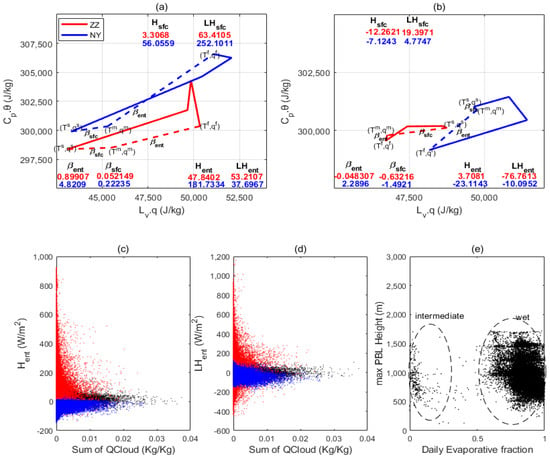
Figure 13.
The mixing diagram framework. (a) The daytime coevolution (00:00–09:00) of and on 20 July 2021 for ZZ (red lines) and NY (blue lines). Also shown are vectors ( and ; dashed lines), slopes ( and ), and energy budget components. (b) is the same as (a) but for the nighttime coevolution (12:00–21:00). (c) The relationship between and clouds for daytime (red scattered), nighttime (blue scattered), and daily (black scattered). (d) is the same as (c) but represents the relationship between and clouds. (e) The relationship of daily EF to maximum PBL height for all grid points over the whole simulation period. Also shown are intermediate, and wet soil locations (dashed circles).
The daytime averaged shows a narrow distribution centered at around 0.4 m3/m3 with a frequency of around 2200 (Figure 14a). and are mostly around 60 W/m2 and 280 W/m2, respectively. Meanwhile, and are mostly around 90 W/m2 and 100 W/m2, respectively. In addition, the latent flux distributions are clearly broader than the heat fluxes. Furthermore, except in the northwest and northeast corners, quite moist soil ( > 0.3 m3/m3) can be observed in most areas during the daytime (Figure 14b). However, the fact that both lower surface heat and latent fluxes can be observed along with the main rainstorm area shows that in addition to soil moisture, the atmospheric forcing has greatly shaped the distribution of surface fluxes during the daytime. Meanwhile, low and relatively higher have dominated the PBL flux contributions from the surface.
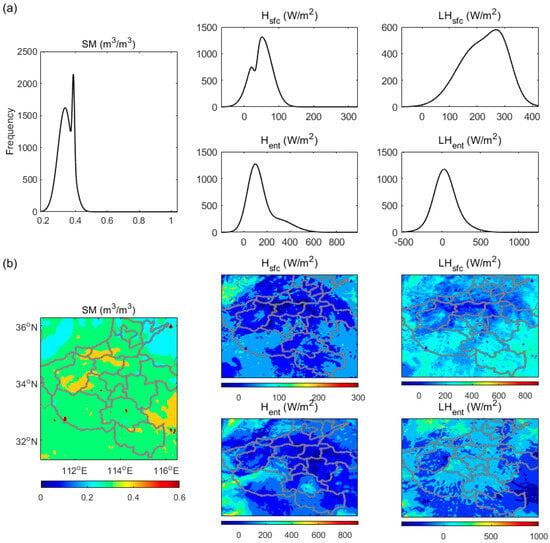
Figure 14.
(a) Frequency distribution of mean soil moisture at 0−10 cm and the PBL energy budgets of MDT during the daytime on 20 July 2021. (b) is the same as (a) but for spatial distribution.
The quite different surface latent or heat flux contribution to PBL for both the ZZ (typically affected by the rainstorm) and NY (non-typical) sites indicate that the magnitude of flux slope has been suppressed by the strong atmospheric forcing during local daytime. The strong with weak shows the quite effective energy transformation of PBL, and it is more pronounced under weak atmospheric forcing (e.g., at the NY site). However, except for latent flux, most nighttime flux contributions are negative. Moreover, in relation to QClouds, the daytime positive entrainment fluxes with a broader distribution than at nighttime indicate the dominant effects of daytime PBL latent contribution on local clouds. While the quite pronounced daily EF (around 0.8) that crosses almost all maximum PBL heights shows the dominant wet evaporation during PBL. These are consistent with the significant noontime PBL moistening indicated by RHT and HCF diagnoses. In addition, besides soil moisture, the atmospheric forcing has greatly shaped the distribution of surface fluxes during the daytime, which is further characterized by low and relatively higher . Generally, the significant daytime weak surface but strong atmosphere flux contributions are quite different from the dry region studies over the United States [28] and Tibet [34,35], and this cloud can be attributed to the quite different weather background.
5.2.5. TCP
TCPLH shows distinct bimodal distributions during the time periods of 00~06, 06~12, and 12~18 when both positive and negative centers with significant frequency can be observed, while the distribution during 18~24 is negatively centered (Figure 15a). Except for the small scattered blocks on the west domain, low negative TCPLH can be observed during 00~06. Next, except for in whole central east region, significant positive TCPLH can be observed during 06~12. Then, the positive TCPLH shrinks to the corners on the south during 12~18. Finally, little scattered positive TCPLH can be observed on the domain margin during 18~24. Clearly, the surface coupling indicated by the positive TCPLH is pronounced from the local afternoon to early night. Furthermore, the TCPSH frequency distributions for different time periods behave consistently with TCPLH but are narrower (Figure 15b). Also, similar spatial distributions of TCPSH but with weaker values compared to TCPLH for different time periods can be observed. In general, the surface coupling indicated by TCPSH and TCPLH are both significant from the local afternoon to early night, and they are especially pronounced in the surrounding areas of the whole central east domain in the local afternoon.
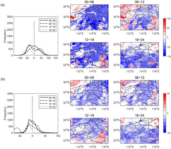
Figure 15.
(a) Frequency and spatial distribution of TCP (units: W/m2) on 20 July 2021 for latent heat flux. (b) is the same as (a) but for the sensible heat flux.
It should be recalled that Low systems developed in the central east domain (Figure 3), where the daytime surface TCP has been clearly suppressed. Overall, the large positive TCP surrounding the central east domain occurs in the local afternoon, indicating that the significant surface coupling feedback is typically positive during this event. Nevertheless, the relatively larger magnitude of TCP compared to previous climatic studies (in which, e.g., TCP varies between −30 and 40 W/m2) [29,30,31] should be attributed to the resolved scale differences between the respective model physics.
5.2.6. SMM
SMM for different periods shows quite different narrow distributions with sharp frequency, the centers of which increase as time goes on (Figure 16). Furthermore, SMM shows a significant northwest-southeast gradient distribution during the period 00~06, and this is opposite to the initial SM gradient. Later, scattered high SMM blocks lay surrounding the whole central east region during 06~12, which is consistent with the TCP of the same period. However, a significant increase in overall SMM for the 12~18 and 18~24 periods can be seen. In particular, decreased SMM in the northern region results in a clear south-north gradient distribution during the 18~24 period. This is obviously related to the northerly developed rainfall late at night.
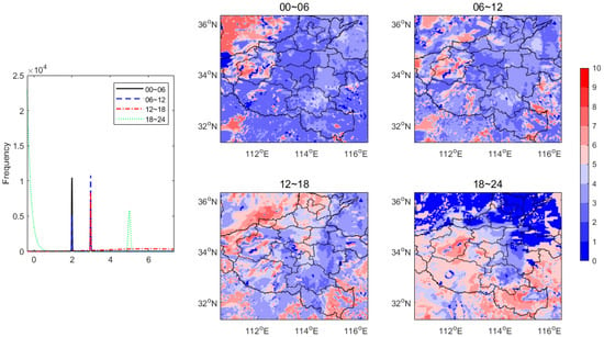
Figure 16.
Frequency and spatial distribution of SMM on 20 July 2021 for surface soil layer.
Overall, the overall SMM increases with time, and daytime SMM is weaker than nighttime. The weak SMM during the daytime should be attributed to the moisture advantage in soil evaporation and/or moist deficits in soil infiltration. Generally, the consistency of SMM with the initial soil gradient and the later developed rainfall show that both the surface soil and upper rainfall shape its spatial distribution, and also the persistence of the anomalies in SM significantly increases after the extreme rainfall. Nevertheless, due to the physical scale difference issues, the SMM magnitude of this study (mostly larger than 2) is relatively larger than in previous climatic studies (in which, e.g., SMM varies between 0 and 1.8) [32].
5.3. The Ensemble Statistical Relations
A study of the between various variations in typical surface and PBL states (within the choice standards described in Section 3) including surface flux slope (), surface temperature and water vapor (, ), 30 m temperature and water vapor (, ), 500 m moist static energy and PBL height (, ), temperature and water vapor at the height averaged between 0 and 1.5 Km (, ), and the 3 h rainfall () resulting from initial soil moisture deviations is conducted to investigate the soil–atmosphere relationship chain during this event. It should be noted that correlations with high confidence where the paired states had the same or opposite physics, or are measured in the same layer or space are excluded to identify the significance in step-wise correlated state pairs (e.g., adjacent states in the LoCo chain). Also, both the domain-averaged (representing the overall domain estimation) and point-wise relationships are evaluated, and, the step-wise relationship chains with significant correlation (e.g., >0.5) and confidence are selected and analyzed.
5.3.1. Spatially Averaged Relations
For dry perturbation (DP), significant negative correlations with high confidence can be found in the distinguished state pairs (, ), (, ), (, ), (, ), (, ), (, ), (, ), (, ), and (, ); however, significant positive correlations with high confidence can be found in the distinguished state pairs (, ), (, ), and (, ) (Figure 17a). The paired states of different layers or space with opposite physics (e.g., humidity and temperature) are further excluded, and that exceed a strength of 0.5 for (, ), (, ), (, ), and (, ) during LoCo chains have been identified (Figure 17b). For wet perturbation (WP), significant negative correlations with high confidence can be found in the distinguished state pairs (, ), (, ), (, ), and (, ); however, significant positive correlations with high confidence can be found in the distinguished state pair (, ) (Figure 17c). Furthermore, that exceeds a strength of 0.5 for (, ), (, ), (, ), and (, ) during the LoCo chains have been identified (Figure 17d).
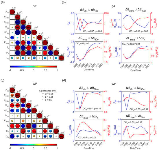
Figure 17.
(a) heat maps of surface flux slope (), surface temperature and water vapor ( and ), 30 m temperature and water vapor ( and ), 500 m moist static energy () and PBL height (), temperature and water vapor at the height averaged between 0 and 1.5 Km ( and ), and 3 h rainfall () for DP. (b) The collaborative variations in the domain-averaged paired factors whose absolute is larger than 0.5 during LoCo chains for DP. The significance level is also shown. (c,d) are the same as (a,b), but for WP.
Clearly, and of DP have fewer correlations (or are less coupled) than those of WP, while in contrast, other states of DP are more informative than those of WP. plays a more significant role than during the step-wise LoCo chains for both DP and WP. And relations are only significant for the surface flux slope for DP. This indicates the significantly different response mechanisms of the atmosphere between DP (e.g., higher PBL with steeper surface flux slope) and WP (e.g., lower PBL with smoother surface flux slope). Moreover, these distinguished surface–PBL relationships for DP (e.g., indirect dry advantage indicated by (, )) and WP (e.g., direct moist advantage indicated by (, )) are similar to those of our previous study of a different region [39], and this could be possibly general for ensemble investigations of rainfall cases with initial moist surface and strong forcing.
5.3.2. Point-Wise Relations
The of (, ) shows a distribution centered at around −0.4 with a frequency of around 600, and the of (, ) shows a distribution with a sharp unimodal centered at around 0.2, while the of (, ) shows a distribution centered at around 0.3 with a frequency of around 500, and of (, ) shows a distribution centered at −0.2 with a frequency of around 550 (Figure 18). Clearly, (, ) and (, ) show a dominant negative correlation, while (, ) and (, ) show opposite behavior. Furthermore, the significant convinced negative (or intense I of Equation (3)) of (, ) is mainly distributed in the east domain along the front of the weather system (Figure 3). Meanwhile, the significant convinced positive of (, ) within many small strip-like aggregations are mainly distributed in the moving path of the synoptic system, which is likely related to the upper and middle layers of the dominant flows (see Section 5.1). Moreover, the significant convinced positive of (, ) within many strip aggregations is mainly distributed in the west domain surrounding the main rainstorm area (null). In addition, the significant convinced negative of (, ) is mainly distributed in a limited area surrounding the rainstorm area, while a convinced positive within many small strip aggregations is distributed in the west away from the rainstorm area.
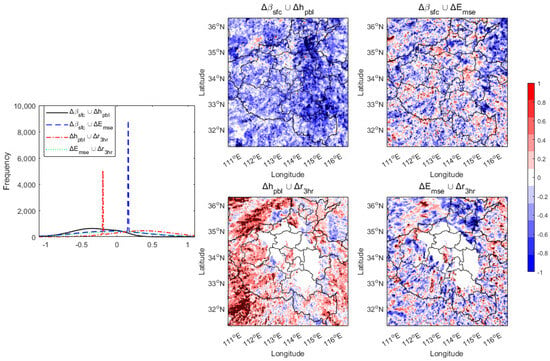
Figure 18.
The frequency (histogram fit), and spatially distributed (shaded) and its significance p (dotted) of different paired variables over the simulation period for DP. The relations between surface flux slope (), 500 m moist static energy(), PBL height(), and 3 h rainfall () are shown.
For DP, the values of (, ) are mainly negative and mostly pronounced in the east region, which is the front end of the precipitation system movement direction, while the of (, ) mainly lies in the regions within the path of the rainstorm’s southwest inflows. The of (, ) are mainly positive and mostly pronounced in the west of the rainfall area, while of (, ) with both negative significance near the rainfall area and positive significance far away from the rainfall area can be observed.
The of (, ) show a distribution centered at −0.3 and the of (, ) show both a broader distribution centered at around 0.1 and a sharp unimodal distribution centered at around 0.4. The of (, ) show both a broader distribution centered around 0.4 and a sharp unimodal distribution centered at around −0.2, while the of (, ) show a distribution centered at −0.1 (Figure 19). Clearly, the dominant for WP is similar to DP but much larger, while the two sharp unimodal distributions indicate the relative significance of their centered values for both (, ) and (, ). Moreover, the spatial distribution of the four pairs for WP is quite similar to that of DP, but the relation intensity of WP is likely narrower and smaller than that of DP.
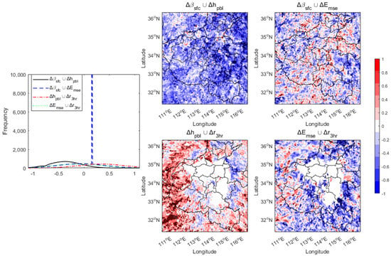
Figure 19.
Same as Figure 18 but for WP.
The dominant of (, ), (, ), (, ), and (, ) for DP and WP are −0.4, 0.2, 0.3, and −0.2, and −0.3, 0.1, 0.3, and −0.2, respectively. This indicates that the point-wise relationship chains are consistent for both DP and WP and that the intensity of the relationship for DP is relatively larger than that for WP, which is consistent with a previous study [39]. Moreover, the conceptual surface–rainfall relationships interfaced by and are both negative, and this might indicate a dominantly negative feedback chain for both DP and WP. Additionally, the significant relationship intensity spatial differences indicate this relationship chain has been highly shaped by the atmospheric forcing (e.g., environmental flows). This is especially pronounced for the chains characterized by the relation intensity among surface flux, PBL height, and rainfall (e.g., east region (, ) and west region (, )).
6. Conclusions
This study simulated a rainstorm of the type experienced on 20 July 2021 over central East China using the CRA40 and GLDAS datasets, and the Noah land surface model coupled with the advanced weather research and forecasting model (WRF, version 3.9.1). Based on this, the gridded planetary boundary layer profiles and ensemble states within soil perturbations were collected to investigate the main land–atmosphere coupling characteristics during the modeled rainstorm using various local coupling metrics and ensemble statistical relations. The main conclusions that can be drawn are as follows.
- The long-lasting Low system with an upper warm flow and a lower strong cold front, the mid-low layer thermodynamic situations, the convection and rainfall spatiotemporal characteristics, and the diurnal surface thermal characteristics of the model are consistent with the available observations. However, the stratospheric (higher than 400 hPa) thermodynamics that relate to the northern developed rainfall and convection, and the over mountain areas have been found to be biased. Except for in the case of the mountain areas, the main characteristics during the mid-low atmospheric layers and the surface have been well documented in this modeled event.
- In CHF, the PBL near the west of the storm center is likely too stable for rain to occur (SRC), and the PBL in the northwest needs additional CTP to trigger convection (TR) while other regions have shown different advantages (e.g., ACA, WSA, and DSA) and are favor of afternoon convection. In terms of RHT, the great contributions to RHT from surface evaporation (SE), PBL warming (BLW), and non-evaporative factors (NE) indicate the dominant roles of these factors in the local PBL clouds that developed before noon, with the SE of around 0.8 and the NE of around 2 being especially significant. In terms of HCF, the noon lower buoyant mixing temperature deficits (e.g., around 274 K) with developing clouds could trigger convection except in the SRC region, while the significant energy transformation of the PBL occurs when the main rainstorm ends and these dominate the development of daytime PBL cloud but with regional differences. In terms of MDT, both the daytime PBL and surface latent energy contributions of around 100 and 280 W/m2, respectively, dominate the relationship between the surface and the PBL clouds; nevertheless, soil moisture and atmospheric forcing greatly shape the daytime distribution of surface fluxes characterized as low entrainment sensible flux () but high entrainment latent flux (). In terms of TCP, surface coupling surrounding the central east domain occurs in the local afternoon and is significant during this event. In terms of SMM, this increases with time, and the comparable distributions of both initial SM and developed rainfall at the end of the day show that both the surface soil and the upper rainfall shape the spatial distribution of SMM.
- Moist static energy () is more general than PBL height () during the step-wise relationship chains for both DP and WP. The deeper PBL with a steeper surface flux slope in DP and the shallower PBL with a smoother surface flux slope in WP are significantly different. However, the point-wise surface–rainfall relationship chains interfaced by or are consistently negative for both DP and WP, while the relation intensity of DP is larger than WP. Nevertheless, the point-wise relationship chains are highly shaped by atmospheric forcing (e.g., environmental flows). This is especially pronounced for the chains characterized by the relationships between surface flux, PBL height, and rainfall.
The dominant local characteristics identified by the abovementioned LoCo metrics are shown in Figure 20. The CHF has determined both the positive (e.g., WSA) and negative (e.g., DSA) feedback [21,22], but the WSA in the east and the ACA have dominated the convection triggering potential, and this shows the dominant surface overall deficits and moistening advantage in the morning (Figure 20a). Both strong moisture evaporation and atmospheric interference (e.g., great daytime SE/BLW and NE in RHT; Figure 20b) before noon enhance the noontime buoyant mixing with higher moist heating deficits (e.g., lower daytime and , but larger in HCF; Figure 20c), which indicates the favorable shallow cloud development surrounding the SRC region [23,24]. However, great entrainment latent fluxes (e.g., higher daytime in MDT) that are most pronounced over the main rainstorm areas (Figure 20d) and likely controlled by the upper flows take over the development of clouds in the early afternoon [28]. The huge energy consumption of greatly developed upper systems results in the higher latent energy deficits of the whole east domain during the late afternoon (e.g., increased and in HCF when the extreme rainfall ends; Figure 11d) [25,26,27]. Moreover, the significant TCP between the noon period and the afternoon also emphasizes the significance of soil–surface coupling in the rainstorm’s surrounding areas (Figure 20e). However, SMM increases as rainfall develops and it is likely matched with TCP in the late afternoon period (Figure 20f). In addition, the relation intensity for DP is greater than that for WP, which should be due to the initial wet soil surface, and the consistent point-wise relationship chains interfaced by moist static energy or PBL height for both WP and DP indicate the overall dominant role of strong atmospheric forcing and negative feedback. Nevertheless, the inconsistent couplings between CHF (e.g., both negative and positive) and ensemble metrics (dominantly negative) show the complex physics of local processes to some extent.
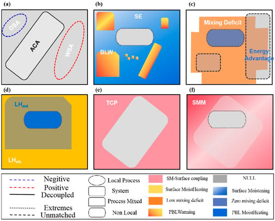
Figure 20.
Summary of the significant daytime local characteristics indicated by the LoCo metrics. (a–f) The CHF, RHT, HCF, MDT, TCP, and SMM, respectively.
It is clear that a WRF model initialized with the CRA40 and GLDAS datasets was well able to simulate various characteristics of synoptic, convection, rainfall, and the surface during this event, especially for the mid-low layers. Moreover, the dominant daytime LoCo characteristics are significant at different times and can be related chronologically (Figure 20). The surface wet soil contributes greatly to the local surface moisture evaporation during the daytime, which then contributes to various PBL advantages for shallow convection development (e.g., increase the early noon PBL warming and/or enhance the noontime buoyant mixing) through local flux allocation; however, the latent flux contribution, which is weak but more significant than the weaker heat flux contribution compared to former studies [34,35] shows an overall suppression of the upper environmental factors (e.g., southwestern low-level inflows of the rainstorm). In contrast, the strong rainstorm forcing significantly shapes the spatial distribution of soil moisture memory, terrestrial coupling parameters, and ensemble statistical relations.
Overall, the local daytime coupling chain during this event can be quantitatively identified as follows: the surface moist heating with developing PBL clouds/rainfall shows the positive response of the atmosphere to the surface from morning until noon, however, the stronger PBL moist heating with significant energy transformation of upper developing systems greatly weakens this response later in the day and further reshapes the surface characteristics, which can be closely related to the background winds. Generally, the overall feedback chain was highly affected by the nonlinear processes during the later period of this event, and the ensemble metrics can identify an overall negative SM–rainfall feedback on a daily scale. This is consistent with the dissipative effect of human-made surfaces in a related study on a greater scale [4].
7. Discussion
Though the LoCo metrics can qualify various local factors by using point-wise simulation profiles under a resolved model grid (4 Km), there are still limitations because of the unsolved multi-scale issues and nonlinearity of physics considering multi-process coexistence. The actual land–atmosphere interaction in nature occurs on much smaller scales, e.g., surface-feature size and atmospheric turbulence scales, and the nonlinear responses, e.g., the upper processes, clearly respond differently to relatively uninformed surfaces, and all the local characteristics are more or less spatiotemporally discontinuous. Therefore, these various inconsistencies in the LoCo metrics show that comparative metrics evaluations are essential to identify the process-distinguished local factors for different regions and/or scales. Additionally, the generality of the chaos of the point-wise ensemble statistics alongside the incompleteness of the spatially averaged relations show that the dominant daily negative surface–rainfall relationship has significant regional uncertainties at finer scales. Therefore, a more detailed investigation of local coupling across different regions should be carried out in the future to enhance the quantitative insights on the typically varied LoCo relationship chain.
For potential real-world applications, the daytime HCF diagnoses have been shown to be reliable indicators for incoming rainfall or convection at a specific location (e.g., for the ZZ and NY sites), and a point-scale weather service could possibly benefit from this. Also, the point-wise CHF and other metric diagnoses with various advantages can be directly referenced for local convection initiation decisions, while the ensemble statistic relations and nighttime LoCo diagnoses should be further studied. In addition, with the development of finer-scale observations of rainfall-related matters [52,53,54], not only finer-scale land–atmosphere coupling assimilation research but also high-resolution radar [55,56] and satellite [57,58,59,60,61,62,63,64,65] data assimilation studies within PBL layers but not completely observed could also benefit from the LoCo metrics for comprehensive data or method evaluation.
Overall, for the heavy rainfall cases, though the model estimations of the consistent daytime moistening of wet surfaces for almost all the metrics can be robust, the abundant evaporation is heavily suppressed during the main rainstorm periods, and the varied pronounced local effects before the rainstorm result in quite different semi-coupled daytime processes during the overall LoCo chain. Similarly, the complete relationships on a daily scale in the ensemble metrics remain empirical and without clear physical identification. Therefore, all the process-typical LoCo diagnoses and the qualitative ensemble diagnoses should be especially enhanced for sharpening the overall feedback chain to clarify various typical local contributions in local rainstorm cases. In particular, the fair or quantitative explanations of the role of local factors in a severe rainstorm event that caused significant disaster and tragedy for both society and individuals and any related typical characteristics [1,2,3,4,66], including LoCo, should be enhanced if they are to play a role in mitigating future risks.
Author Contributions
Conceptualization, methodology, validation, formal analysis, Y.G.; investigation, resources, and data curation, C.S.; writing—original draft preparation, C.S.; writing—review and editing, A.S. visualization, A.S.; supervision, C.S.; project administration, A.S.; funding acquisition, C.S. All authors have read and agreed to the published version of the manuscript.
Funding
This research was funded by the Science and Technology Project on Innovation Ecosystem Construction at Zhengzhou Supercomputing Center in Henan province (grant number: 201400210800), the China Environmental Protection Foundation Blue Mountain Project (grant number: CEPFQS202169-28), the China Meteorological Administration Meteorological Observation Centre “Chipset Plan” (Xiaoman I) and “Incubation Project” (MOCFH202309).
Institutional Review Board Statement
Not applicable.
Informed Consent Statement
Not applicable.
Data Availability Statement
The data presented in this study are available on request.
Acknowledgments
We would like to express our gratitude to the China Meteorological Administration Meteorological Observation Centre and the Henan Meteorological Bureau for their support in carrying out this study. We would like to thank the anonymous reviewers for their valuable feedback, which greatly improved the quality of this article. And we also would like to give our many thanks to those who have made their efforts in advancing this work, and the fellow travelers along the way.
Conflicts of Interest
The authors declare no conflict of interest.
References
- Liu, X.; Yang, M.; Wang, H.; Liu, K.; Dong, N.; Wang, H.J.; Zhang, L.M.; Fan, W. Moisture sources and atmospheric circulation associated with the record-breaking rainstorm over Zhengzhou city in July 2021. Nat. Hazards 2023, 116, 817–836. [Google Scholar] [CrossRef]
- Yang, Y.; Gao, T.; Xie, L.; Zhang, R.H.; Zhang, W.; Xu, H.X.; Cao, F.Q.; Chen, B. Tropical cyclone over the western Pacific triggers the record-breaking “21/7” extreme rainfall in Henan, central-eastern China. Environ. Res. Lett. 2022, 17, 124003. [Google Scholar]
- Xue, M. Preface to the Special Collection on the July 2021 Zhengzhou, Henan Extreme Rainfall Event. Adv. Atmos. Sci. 2023, 40, 335–336. [Google Scholar] [CrossRef]
- Luo, Y.; Zhang, J.; Yu, M.; Liang, X.D.; Xia, R.D.; Gao, Y.Y.; Gao, X.Y.; Yin, J.F. On the Influences of Urbanization on the Extreme Rainfall over Zhengzhou on 20 July 2021: A Convection-Permitting Ensemble Modeling Study. Adv. Atmos. Sci. 2023, 40, 393–409. [Google Scholar] [CrossRef]
- Betts, A.K. Land-surface-atmosphere coupling in observations and models. J. Adv. Model. Earth Sys. 2009, 1, 4. [Google Scholar] [CrossRef]
- Song, Y.M.; Guo, W.D.; Zhang, Y.C. Numerical study of impacts of soil moisture on the diurnal and seasonal cycles of sensible/latent heat fluxes over semi-arid region. Adv. Atmos. Sci. 2009, 26, 319–326. [Google Scholar] [CrossRef]
- Beljaars, A.; Viterbo, P.; Miller, M.; Betts, A.K. The anomalous rainfall over the United States during July 1993: Sensitivity to land surface parameterization and SM anomalies. Mon. Wea. Rev. 1996, 124, 362–383. [Google Scholar] [CrossRef]
- Koster, R.D.; Suarez, M.J.; Higgins, R.W.; Van den Dool, H.M. Observational evidence that soil moisture variations affect precipitation, Geophys. Res. Lett. 2003, 30, 1241. [Google Scholar] [CrossRef]
- Liu, W.; Zhang, Q.; Li, C.; Xu, L.; Xiao, W. The influence of soil moisture on convective activity: A review. Theor. Appl. Climatol. 2022, 149, 221–232. [Google Scholar] [CrossRef]
- Koster, R.D.; Dirmeyer, P.A.; Guo, Z.; Bonan, G.; Chan, E.; Cox, P.; Gordon, B.; Kanae, S.; Kowalczyk, E.; Lawreencce, D.; et al. Regions of Strong Coupling Between Soil Moisture and Precipitation. Science 2004, 305, 1138–1140. [Google Scholar] [CrossRef]
- Guillod, B.P.; Orlowsky, B.; Miralles, D.G.; Teuling, A.J.; Seneviratne, S. Reconciling spatial and temporal soil moisture effects on afternoon rainfall. Nat. Commun. 2015, 6, 6443. [Google Scholar] [CrossRef] [PubMed]
- Hsu, H.; Dirmeyer, P.A. Soil moisture-evaporation coupling shifts into new gears under increasing CO2. Nat. Commun. 2023, 14, 1162. [Google Scholar] [CrossRef] [PubMed]
- Zhang, R.; Xu, X.; Guo, J.; Sheng, Z. The ratio distribution of evapotranspiration to precipitation well related with soil thickness of Karst watershed in southwest China. J. Geophys. Res. Atmos. 2023, 128, e2022JD037951. [Google Scholar] [CrossRef]
- Divyansh, C.; Francina, D.; Christopher, M.T.; Cornelia, K.; Stephen, W.N. Dry-to-Wet Soil Gradients Enhance Convection and Rainfall over Subtropical South America. J. Hydrometeor. 2023. [Google Scholar] [CrossRef]
- Quintanar, A.; Mahmood, R.; Mofley, M.; Yan, J.; Loughrin, J.; Lovanh, N. Simulation of boundary layer trajectory dispersion sensitivity to soil moisture conditions: MM5 and Noah-based investigation. Atmos. Environ. 2009, 43, 3774–3785. [Google Scholar] [CrossRef]
- Suarez, A.; Mahmood, R.; Quintanar, A.; Beltrán-Przekurat, A.; Pielke Sr, R. A comparison of the MM5 and the RAMS simulations for land-atmosphere interactions under varying soil moisture. Tellus 2014, 66, 178–183. [Google Scholar]
- Mahmood, R.; Leeper, R.; Quintanar, A. Sensitivity of planetary boundary layer atmosphere to historical and future changes of land use/land cover, vegetation fraction, and soil moisture in Western Kentucky, USA. Global Planet. Chang. 2011, 78, 36–53. [Google Scholar] [CrossRef]
- Leeper, R.; Mahmood, R.; Quintanar, A. Influence of Karst Landscape on Planetary Boundary Layer Atmosphere: A Weather Research and Forecasting (WRF) Model-Based Investigation. J. Hydrometeor. 2011, 12, 1512–1529. [Google Scholar] [CrossRef]
- Simon, J.S.; Bragg, A.D.; Dirmeyer, P.A.; Chaney, N.W. Semi-coupling of a field-scale resolving land-surface model and WRF-LES to investigate the influence of land-surface heterogeneity on cloud development. J. Adv. Model. Earth Sys. 2021, 13, e2021MS002602. [Google Scholar] [CrossRef]
- Santanello, J.A.; Lawston, P.; Kumar, S.; Dennis, E. Understanding the impacts of soil moisture initial conditions on NWP in the context of land–atmosphere coupling. J. Hydrometeor. 2019, 20, 793–819. [Google Scholar] [CrossRef]
- Findell, K.L.; Eltahir, E. Atmospheric controls on soil moisture-boundary layer interactions. Part I: Framework development. J. Hydrometeor. 2003, 4, 552–569. [Google Scholar] [CrossRef]
- Findell, K.L.; Eltahir, E. Atmospheric Controls on Soil Moisture–Boundary Layer Interactions. Part II: Feedbacks within the Continental United States. J. Hydrometeor. 2003, 4, 570–583. [Google Scholar] [CrossRef]
- Ek, M.; Mahrt, L. Daytime evolution of relative humidity at the boundary-layer top. Mon. Wea. Rev. 1994, 122, 2709–2721. [Google Scholar] [CrossRef]
- Ek, M.; Holtslag, A. Influence of soil moisture on boundary cloud development. J. Hydrometeor. 2004, 5, 86–99. [Google Scholar] [CrossRef]
- Tawfik, A.B.; Dirmeyer, P.A. A process-based framework for quantifying the atmospheric preconditioning of surface-triggered convection. Geophys. Res. Lett. 2014, 41, 173–178. [Google Scholar] [CrossRef]
- Tawfik, A.B.; Dirmeyer, P.A.; Santanello, J.A. The heated condensation framework. part i: Description and southern great plains case study. J. Hydrometeor. 2015, 16, 150603105509002. [Google Scholar] [CrossRef]
- Tawfik, A.B.; Dirmeyer, P.A.; Santanello, J.A. The heated condensation framework. part ii: Climatological behavior of convective initiation and land-atmosphere coupling over the conterminous united states. J. Hydrometeor. 2015, 16, 150603105509002. [Google Scholar] [CrossRef]
- Santanello, J.A.; Peters-Lidard, C.D.; Kumar, S. A modeling and observational framework for diagnosing local land–atmosphere coupling on diurnal time scales. J. Hydrometeor. 2009, 10, 577–599. [Google Scholar] [CrossRef]
- Delworth, T.L.; Manabe, S. The influence of potential evaporation on the variabilities of simulated soil wetness and climate. J. Climate 1988, 1, 523–547. [Google Scholar] [CrossRef]
- Delworth, T.L.; Manabe, S. The influence of soil wetness on near-surface atmospheric variability. J. Climate 1989, 2, 1447–1462. [Google Scholar] [CrossRef]
- Dirmeyer, P.A. The terrestrial segment of soil moisture–climate coupling. Geophys. Res. Lett. 2011, 38, L16702. [Google Scholar] [CrossRef]
- Guo, Z.C.; Dirmeyer, P.A.; Koster, R.D.; Sud, Y.; Bonan, G.; Oleson, K.; Chan, E.; Versghy, D.; Cox, P.; Gordon, C.T.; et al. GLACE: The Global Land–Atmosphere Coupling Experiment Part II: Analysis. J. Hydrometeor. 2006, 7, 611–625. [Google Scholar] [CrossRef]
- Santanello, J.A.; Dirmeyer, P.A.; Ferguson, C.R.; Findell, K.; Tawfik, A.; Berg, A.; Ek, M.; Gentine, P.; Guillod, B.; Heerwaardeen, C.; et al. Land–atmosphere interactions: The LoCo perspective. BAMS 2018, 99, 1253–1272. [Google Scholar] [CrossRef]
- Sun, G.; Hu, Z.; Ma, Y.; Xie, Z.; Yang, S.; Wang, J. Analysis of local land-atmosphere coupling in rainy season over a typical underlying surface in Tibetan Plateau based on field measurements and ERA5. Atmos. Res. 2020, 243, 105025. [Google Scholar] [CrossRef]
- Sun, G.; Hu, Z.; Ma, Y.; Xie, Z.; Yang, S. Simulation analysis of local land-atmosphere coupling in rainy season over a typical underlying surface in Tibetan Plateau. Hydrol. Earth Sys. Sci. 2020, 24, 5937–5951. [Google Scholar] [CrossRef]
- Abdolghafoorian, A.; Dirmeyer, P.A. Validating the land-atmosphere coupling behavior in weather and climate models using observationally based global products. J. Hydrometeor. 2021, 22, 1507–1523. [Google Scholar] [CrossRef]
- Zhao, C.; Meng, X.; Li, Y.; Lyu, S.; Guo, J.; Liu, H. Impact of soil moisture on afternoon convection triggering over the Tibetan Plateau based on 1-D boundary layer model. J. Geophys. Res. Atmos. 2022, 127, e2021JD035591. [Google Scholar] [CrossRef]
- Quintanar, A.; Mahmood, R. Ensemble forecast spread induced by soil moisture changes over mid-south and neighbouring mid-western region of the USA. Tellus 2012, 64, 145–153. [Google Scholar] [CrossRef]
- Min, J.Z.; Guo, Y.K.; Wang, G.J. Impacts of soil moisture on typical frontal rainstorm in yangtze river basin. Atmosphere 2016, 7, 42. [Google Scholar] [CrossRef]
- Tewari, M.; Chen, F.; Wang, W.; Dudhia, J.; LeMone, M.A.; Mitchell, K.; Ek, M.; Gayno, G.; Wegiel, J.; Cuenca, R.H. Implementation and verification of the unified NOAH land surface model in the WRF model. In Proceedings of the 20th Conference on Weather Analysis and Forecasting/16th Conference on Numerical Weather Prediction, Seattle, WA, USA, 12–16 January 2004; pp. 11–15. [Google Scholar]
- Skamarock, W.C.; Klemp, J.B.; Dudhia, J.; Gill, D.O.; Barker, D.; Duda, M.G.; Huang, X.Y.; Wang, W.; Powers, J.G. A Description of the Advanced Research WRF Version 3 (No. NCAR/TN-475+STR). NCAR Tech. Note 2008, 475, 113. [Google Scholar]
- Thompson, G.; Field, P.; Rasmussen, R.; Hall, W. Explicit Forecasts of Winter Precipitation Using an Improved Bulk Microphysics Scheme. Part II: Implementation of a New Snow Parameterization. Mon. Wea. Rev. 2008, 136, 5095–5115. [Google Scholar] [CrossRef]
- Iacono, M.J.; Delamere, J.S.; Mlawer, E.J.; Shephard, M.W.; Clough, S.A.; Collins, W.D. Radiative forcing by long–lived greenhouse gases: Calculations with the AER radiative transfer models. J. Geophys. Res. Atmos. 2008, 113, D13103. [Google Scholar] [CrossRef]
- Kain, J.S. The Kain–Fritsch convective parameterization: An update. J. Appl. Meteor. 2004, 43, 170–181. [Google Scholar] [CrossRef]
- Jimenez, P.A.; Dudhia, J.; Gonzalez–Rouco, J.F.; Navarro, J.; Montavez, J.P.; Garcia–Bustamante, E. A revised scheme for the WRF surface layer formulation. Mon. Wea. Rev. 2012, 140, 898–918. [Google Scholar] [CrossRef]
- Hong, S.Y.; Noh, Y.; Dudhia, J. A new vertical diffusion package with an explicit treatment of entrainment processes. Mon. Wea. Rev. 2006, 134, 2318–2341. [Google Scholar] [CrossRef]
- Andras, H.; Paul, B.; Gionata, B.; Dick, D.; Hans, H.; Joaquin, M.S.; Iryna, R.; Adrian, S.; Cornel, S. The impact of observations in the ECMWF latest reanalysis system. In Proceedings of the WMO Workshop, Shanghai, China, 10–13 May 2016. [Google Scholar]
- Wang, M.Y.; Yao, S.; Jiang, L.P.; Liu, Z.Q.; Shi, C.X.; Hu, K.X.; Zhang, T.; Zhang, Z.S.; Liu, J.W. Collection and Pre-Processing of Satellite Remote-Sensing Data in CRA-40 (CMA’s Global Atmospheric ReAnalysis). Adv. Meteoro. Sci. Tech. 2018, 8, 158–163. (In Chinese) [Google Scholar]
- Beaudoing, H.; Rodell, M. NASA/GSFC/HSL(2020), GLDAS Noah Land Surface Model L4 3 hourly 0.25 × 0.25 degree V2.1, Greenbelt, Maryland, USA, Goddard Earth Sciences Data and Information Services Center (GES DISC). Available online: https://disc.gsfc.nasa.gov/ (accessed on 4 September 2023).
- Sun, S.; Shi, C.; Pan, Y.; Bai, L.; Xu, B.; Zhang, T.; Han, S.; Jiang, L. Applicability assessment of the 1998-2018 CLDAS multi-source precipitation fusion dataset over China. J. Meteoro. Res. 2020, 34, 879–892. [Google Scholar] [CrossRef]
- Fieller, E.C.; Hartley, H.O.; Pearson, E.S. Tests for rank correlation coefficients. I. Biometrika 1957, 44, 470–481. [Google Scholar] [CrossRef]
- Ghosh, K.G. Analysis of Rainfall Trends and its Spatial Patterns During the Last Century over the Gangetic West Bengal, Eastern India. J. Geovis. Spat. Anal. 2018, 2, 15. [Google Scholar] [CrossRef]
- Mantovani, J.R.; Bueno, G.T.; Alcântara, E.; Park, E.; Cunha, A.; Londee, L.; Massi, K.; Marengo, J. Novel Landslide Susceptibility Mapping Based on Multi-criteria Decision-Making in Ouro Preto, Brazil. J. Geovis. Spat. Anal. 2023, 7, 7. [Google Scholar] [CrossRef]
- Filonchyk, M.; Yan, H.; Zhang, Z.; Yang, S.; Li, W.; Li, Y. Combined use of satellite and surface observations to study aerosol optical depth in different regions of China. Sci. Rep. 2019, 9, 6174. [Google Scholar] [CrossRef]
- Shen, F.; Min, J.; Xu, D. Assimilation of radar radial velocity data with the WRF Hybrid ETKF–3DVAR system for the prediction of Hurricane Ike (2008). Atmos. Res. 2016, 169, 127–138. [Google Scholar] [CrossRef]
- Shen, F.; Xu, D.; Min, J.; Chu, Z.; Li, X. Assimilation of radar radial velocity data with the WRF hybrid 4DEnVar system for the prediction of hurricane Ike (2008). Atmos. Res. 2020, 234, 104771. [Google Scholar] [CrossRef]
- Xu, D.; Liu, Z.; Huang, X.Y.; Min, J.; Wang, H. Impact of assimilating IASI radiance observations on forecasts of two tropical cyclones. Meteorol. Atmos. Phys. 2013, 122, 1–18. [Google Scholar] [CrossRef]
- Shen, F.; Min, J. Assimilating AMSU-A radiance data with the WRF Hybrid En3DVAR system for track predictions of Typhoon Megi (2010). Adv. Atmos. Sci. 2015, 32, 1231–1243. [Google Scholar] [CrossRef]
- Xu, D.; Min, J.; Shen, F.; Ban, J.; Chen, P. Assimilation of MWHS radiance data from the FY–3B satellite with the WRF Hybrid–3DVAR system for the forecasting of binary typhoons. J. Adv. Model. Earth Sys. 2016, 8, 1014–1028. [Google Scholar] [CrossRef]
- Xu, D.; Liu, Z.; Fan, S.; Chen, M.; Shen, F. Assimilating all-sky infrared radiances from Himawari-8 using the 3DVar method for the prediction of a severe storm over North China. Adv. Atmos. Sci. 2021, 38, 661–676. [Google Scholar] [CrossRef]
- Xu, D.; Zhang, X.; Liu, Z.; Shen, F. All-sky infrared radiance data assimilation of FY-4A AGRI with different physical parameterizations for the prediction of an extremely heavy rainfall event. Atmos. Res. 2023, 293, 106898. [Google Scholar] [CrossRef]
- Shen, F.; Xu, D.; Li, H.; Min, J.; Liu, R. Assimilation of GPM Microwave Imager Radiance data with the WRF hybrid 3DEnVar system for the prediction of Typhoon Chan-hom (2015). Atmos. Res. 2021, 251, 105422. [Google Scholar] [CrossRef]
- Song, L.; Shen, F.; Shao, C.; Shu, A.; Zhu, L. Impacts of 3DEnVar-Based FY-3D MWHS-2 Radiance Assimilation on Numerical Simulations of Landfalling Typhoon Ampil (2018). Remote Sens. 2022, 14, 6037. [Google Scholar] [CrossRef]
- Zhang, X.; Xu, D.; Liu, R.; Shen, F. Impacts of FY-4A AGRI Radiance Data Assimilation on the Forecast of the Super Typhoon “In-Fa” (2021). Remote Sens. 2022, 14, 4718. [Google Scholar] [CrossRef]
- Shu, A.; Shen, F.; Jiang, L.; Zhang, T.; Xu, D. Assimilation of Clear-sky FY-4A AGRI radiances within the WRFDA system for the prediction of a landfalling Typhoon Hagupit (2020). Atmos. Res. 2022, 283, 106556. [Google Scholar] [CrossRef]
- Liu, Y.; Yang, Y. Spatial-temporal variability pattern of multi-depth soil moisture jointly driven by climatic and human factors in China. J. Hydro. 2023, 619, 129313. [Google Scholar] [CrossRef]
Disclaimer/Publisher’s Note: The statements, opinions and data contained in all publications are solely those of the individual author(s) and contributor(s) and not of MDPI and/or the editor(s). MDPI and/or the editor(s) disclaim responsibility for any injury to people or property resulting from any ideas, methods, instructions or products referred to in the content. |
© 2023 by the authors. Licensee MDPI, Basel, Switzerland. This article is an open access article distributed under the terms and conditions of the Creative Commons Attribution (CC BY) license (https://creativecommons.org/licenses/by/4.0/).