Article

A Novel Combined Model for Air Quality Index Forecasting in Changchun

School of Science, Changchun University, Changchun 130022, China
*
Author to whom correspondence should be addressed.
Atmosphere 2023, 14(10), 1475; https://doi.org/10.3390/atmos14101475
Submission received: 17 August 2023 / Revised: 22 September 2023 / Accepted: 22 September 2023 / Published: 24 September 2023
(This article belongs to the Section Air Quality)

Abstract

:
With the rapid development of the economy and continuous improvement in people’s living standards, the predictions of the air quality index have attracted wide attention. In this paper, a new feature selection method (Pearson-MI) and a combined model construction method (modified inverse variance method) were proposed to study the air quality index (AQI) and its influencing factors in Changchun. The Pearson-MI method selects the factors that affect the AQI of Changchun City from many influencing factors. This method reduces the RMSE of the LSTM model and XGBoost model by 27% and 5% and the MAE by 41% and 5%, respectively. A model that combines XGBoost, SVR, RF, and LSTM was constructed using the inverse variance method to predict the air quality index of Changchun City. The modified combined model resulted in a 2% reduction in RMSE and a 0.6% reduction in MAE compared with the unmodified combined model. The numerical results of our study show that the prediction accuracy of the modified combined model is obviously higher than that of the basic model, and the prediction accuracy is further improved under the Pearson-MI feature selection.

1. Introduction

1.1. Background and Motivation

Air is essential for the survival and development of all life on Earth, and it affects a person’s health as well as the economy [1]. Air quality is largely determined by natural and human activities, such as volcanic eruptions, forest fires, climate change, ozone hole, industrialization, urbanization, and transportation emissions [2]. Many pollutants can be found in the atmosphere, such as SO2, NO2, CO2, NO, CO, NO, PM2.5, and PM10. A large amount of research on air pollution forecasting and air quality index forecasting around the world has focused on pollutant forecasting. Air pollution is both an environmental and a public health issue, especially in developing countries. Short- or long-term exposure to polluted environments can have serious adverse effects on human health, and air pollution is responsible for increased mortality and hospitalization rates, reduced life expectancy, and epidemics of asthma and allergies [3]. Air pollution is also an important factor affecting climate change and ecohydrological processes. One study found that there can be significant economic costs for individuals and society due to air pollution [4].
With the rapid development of the economy and continuous improvements in people’s living standards, the study of air quality has received much attention. Only when we use objective and scientific air quality assessment methods can we really mobilize the enthusiasm and scientific nature of local governments to control air pollution [5]. Changchun is one of the central cities in northeast China; it is very representative of an industrial base [6]. Accurate prediction of the AQI in Changchun could not only provide a scientific basis for the government to formulate and optimize environmental management policies, but it could also provide important early warning information for residents so that they can take appropriate protective measures during the peak pollution period [7]. At the same time, excellent AQI prediction methods can be used to evaluate the effect of air quality improvements. Therefore, the establishment of an air quality prediction model in Changchun has an important reference significance for the environmental monitoring of industrial cities in China.
According to the concentration of air pollutants, the air quality index is a comprehensive index used to reflect the quality of the atmospheric environment [8]. The air quality index and corresponding grades are shown in Table 1.

1.2. Related Work

Artificial intelligence algorithms are playing an increasingly important role in environmental detection. For example, in hydrology, artificial intelligence, and climate detection, the use of corresponding algorithms can achieve good prediction results [9,10,11].
Establishing a scientific system of influencing factors is an important part of air quality research. Luo et al. (2022) [12] have shown that although air pollution is caused by pollutants being discharged into the atmosphere, the actual observed pollution level is affected by meteorological conditions because they can affect the diffusion of pollutants. According to the air quality status and spatial distribution characteristics of 113 key environmental protection cities in China, Zhang and Lin (2022) [13] analyzed the main socio-economic factors affecting changes in air quality. Zhao et al. (2021) [14] studied the relationship between the concentration of six pollutants in the air and thirteen economic and social factors, consequently proposing suggestions for improving air quality.
Different feature selection schemes may have different impacts on model accuracy. Aly et al. (2023) [15] proposed a feature selection method based on a decision tree algorithm and enhanced Gini index. The results show that this method greatly reduces the data dimension and avoids the problem of over-fitting. Mohamed et al. (2022) [16] obtained a feature selection method, FWA-FS, based on the fireworks algorithm. Experimental results show that FWA-FS can significantly improve classification performance. Sethi et al. (2021) [17] presented a feature selection method based on minimum absolute selection and a contraction operator to predict air quality. Their results show that the feature subset extracted using feature selection performs better than the complete dataset and the subset extracted via LASSO regression.
Traditional machine learning algorithms have been able to better predict the air quality index, but traditional machine learning algorithms have limitations. That is, the same model has significantly different effects on different data. Maltare Nilesh et al. (2023) [18] used various machine learning methods such as SARIMA, SVM, and LSTM to predict the air quality index in Ahmedabad, Gujarat, India. Their results show that the support vector machine algorithm of the RBF kernel model has a better prediction effect compared with other models. Shi et al. (2023) [19] established a new grey prediction model to predict the air quality in Shijiazhuang. Their experimental results outline that the model shows a good prediction performance and generalization ability. Singh et al. (2023) [20] used satellite data to discuss the changes in the AQI in India during the COVID-19 pandemic; they used the most advanced statistical and deep learning methods to predict the AQI. Their results show that the short-term AQI prediction accuracy of Holt–Winter shows a better performance. Wong Y J et al. (2023) [21] used tree-based models and linear models to study nitrogen dioxide and ozone concentrations and found that the performance of random forest and GBM models was better than that of GAM and GLM models.
In order to overcome the limitations of a single prediction model, building a fusion prediction model is an effective solution for the prediction of the air quality index. Xu et al. (2021) [22] proposed an improved seagull optimization algorithm and combined it with support vector regression to establish a hybrid prediction model. Phruksahiran (2021) [23] introduced an integrated prediction method combined with a machine learning algorithm to investigate the prediction of the concentration of atmospheric pollutants. Their results show that this method is helpful in enhancing the accuracy of air quality index prediction. Yan et al. (2021) [24] predicted the air quality index of Beijing, and their results showed that CNN-LSTM and LSTM were generally superior to CNN and BPNN.
In addition, in the process of model fitting, K-fold cross-validation can be added to avoid over-fitting and reduce the fitting effect caused by insufficient data [25]. At the same time, grid search can be used to select the optimal parameters of the model so that the model has the best fitting effect [26].

1.3. Our Contribution

The contributions of the paper can be summarized as follows.
  • We propose the Pearson-MI method to analyze the importance of various features. This method can effectively obtain the contributions of features during the training process and perform feature screening and filtering on the prediction model.
  • This paper uses a variety of models to predict the air quality index. Using XGBoost, support vector regression (SVR), random forest, and LSTM can reduce the contingency and inadaptability of the prediction of a single model.
  • In this paper, a variety of models are combined, and the model is weighted by the modified reciprocal variance method. This can further improve the predictive performance of the model.
  • Numerical experiments show that the combined model based on Pearson-MI feature selection and an improved inverse variance method to weigh the model shows a good performance in the prediction of the air quality index.
The remainder of this paper is structured as follows: In Section 2, we introduce the Pearson-MI method and the modified inverse variance method in detail. In Section 3, we take Changchun City as an example, introduce the data source, and describe data preprocessing, feature selection, and model prediction in detail. Finally, in Section 4, we summarize our research content.
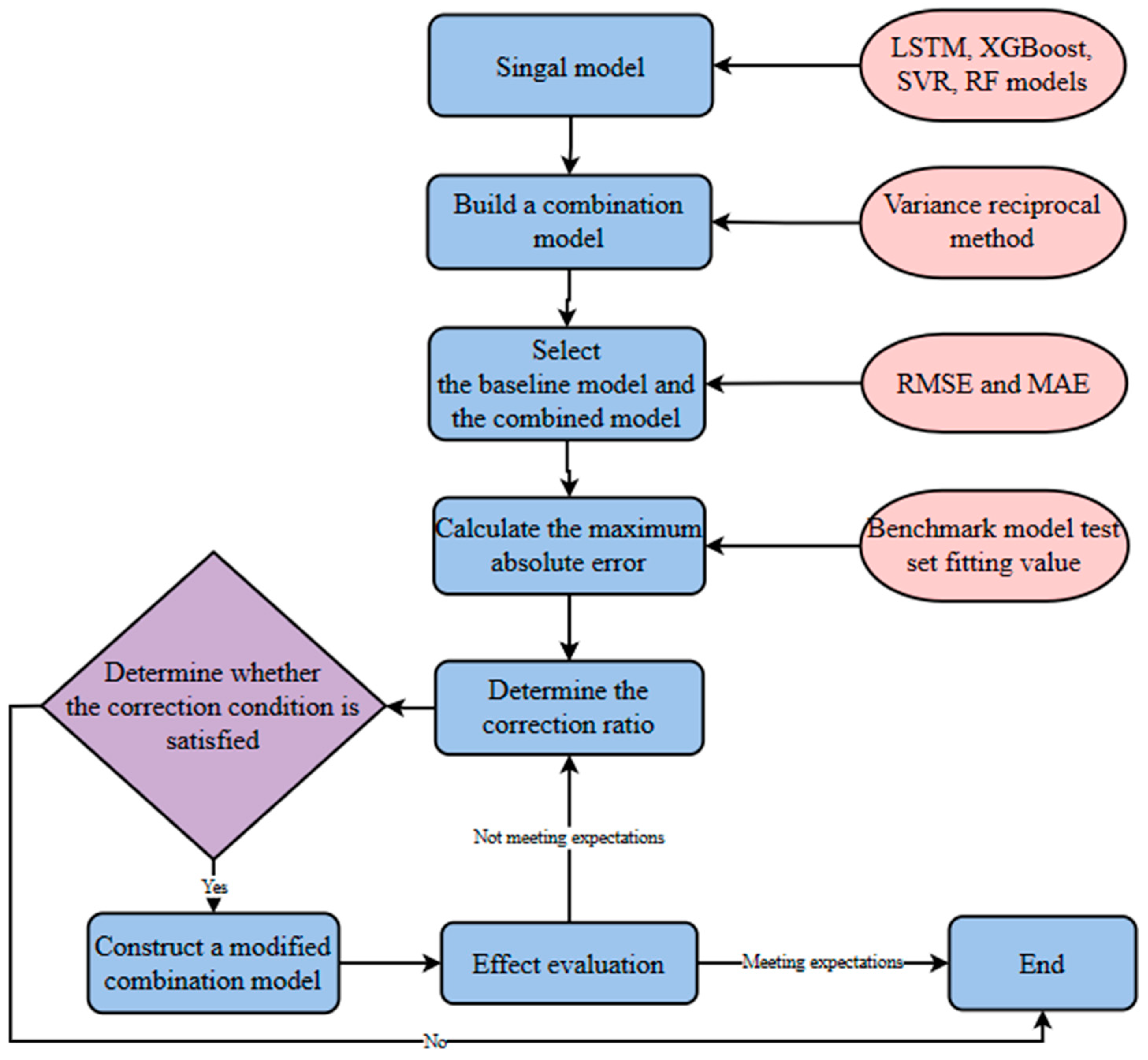
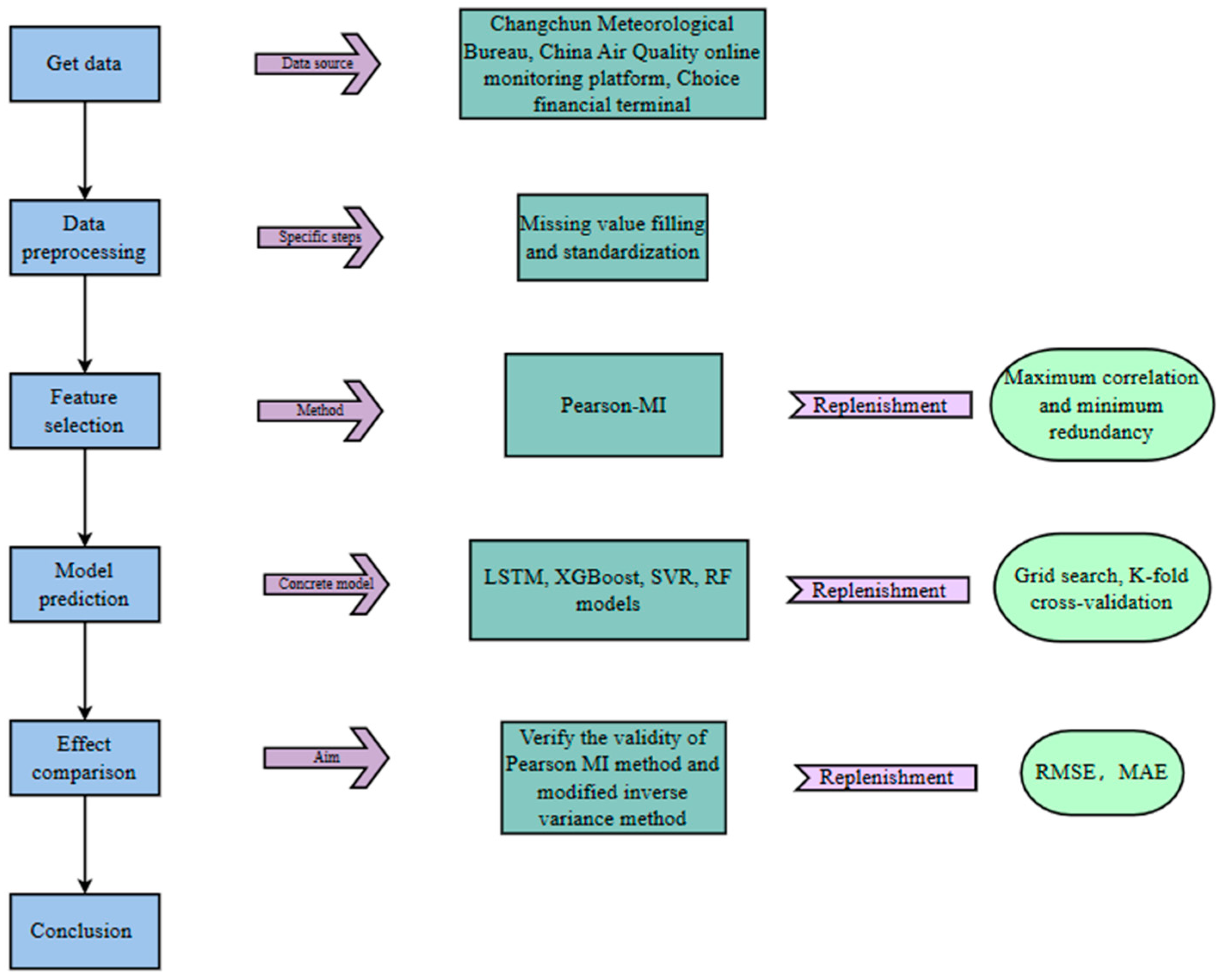
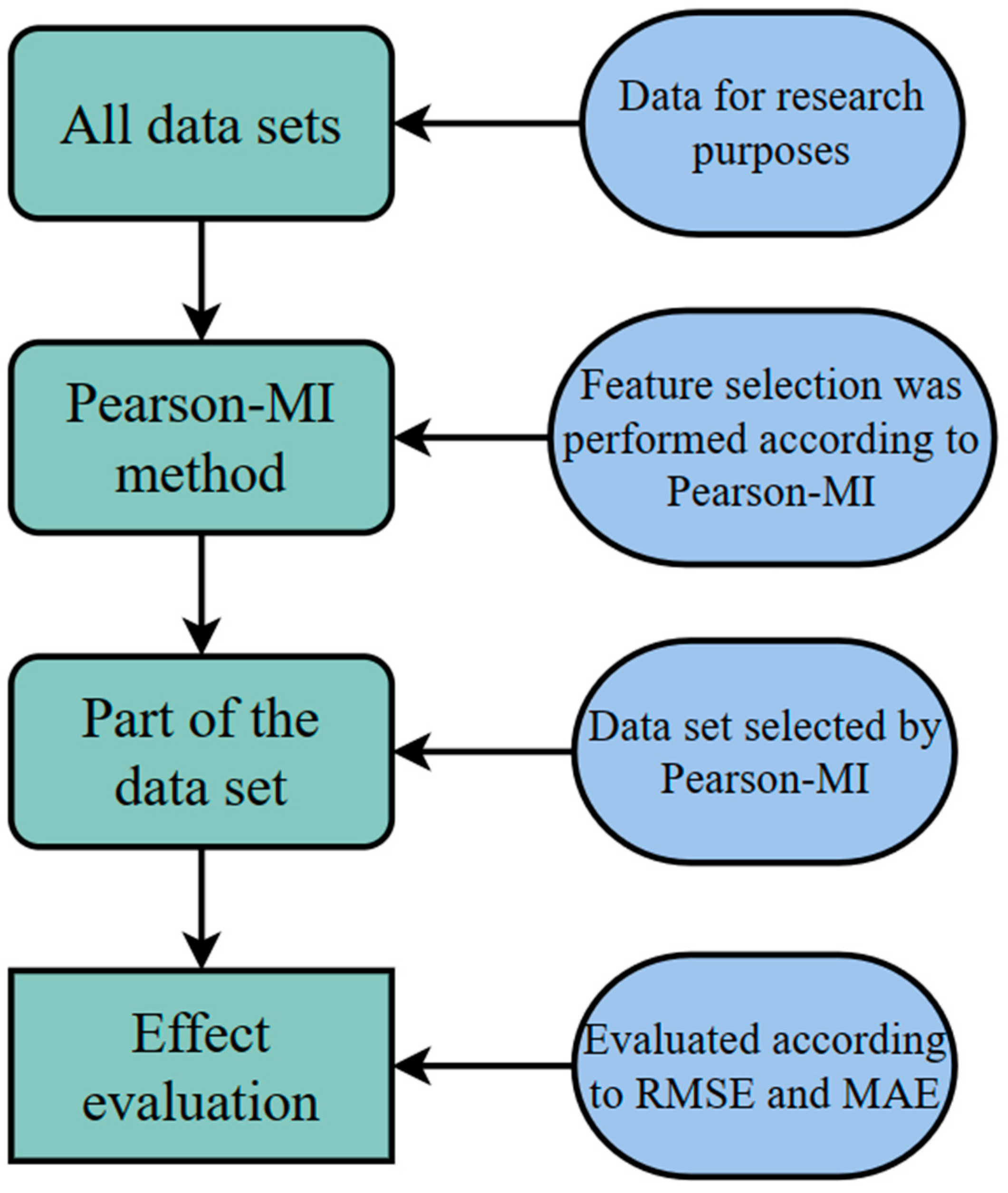
The overall framework of this article is outlined in Figure 1.

2. Methodology and Materials

2.1. Pearson-MI Method

Based on the Pearson correlation coefficient and mutual information, the Pearson-MI method was constructed using the principle of maximum correlation and minimum redundancy, which is used for feature selection. The steps are given as follows.
Step 1. Calculate the correlation between independent variables and dependent variables, including linear correlation and nonlinear correlation. The measurement indices are the Pearson correlation coefficient and mutual information.
ρ = c o v ( A i , B ) σ A i σ B ,
D i = I ( A i ; B ) .
where ρ is the Pearson correlation coefficient used to measure the linear correlation between variables; A i is the independent variable, indicating that i-th is the influencing factor; B is the dependent variable, namely the air quality index; cov is the covariance between variables, and σ is the standard deviation. D i and I are mutual information to measure the nonlinear correlation between variables.
Step 2. Eliminate independent variables with a low correlation with dependent variables (maximum correlation).
Step 3. Calculate the linear correlation between independent variables after being eliminated in Step 2, and the measurement index is the Pearson correlation coefficient.
Step 4. Take out independent variables with a high correlation as alternative variables. If the alternative variables contain similar indicators, only one is reserved. The remaining variables are required.
Step 5. Calculate the mutual information of the required variable and the combination of various features in the required variable and the alternative variable.
Step 6. Select the feature combination with the smallest mutual information as the feature after feature selection.
Step 7. Evaluate the effect. This is used to judge the validity of feature selection.
The following are the definitions of some nouns.
Dependent variable: air quality index.
Independent variables: the various factors that affect the air quality index, also known as influencing factors.
Similar indicators: average temperature, highest temperature, and lowest air temperature are similar indicators, or there is a significant correlation between a certain independent variable and other variables.
Required variable: a variable selected according to the Pearson-MI method that must be used as an influencing factor.
Alternative variables: variables that may be selected as influencing factors based on the Pearson-MI method.
A flowchart of the Pearson-MI method for feature selection is shown in Figure 2:

2.2. Modified Reciprocal Variance Method

The main idea of the reciprocal variance method is that the weight of each model is distributed according to the reciprocal of its variance. That is, the smaller the variance, the greater the weight of the model. This is because the variance reflects the dispersion of data, and the smaller the variance, the more stable the data are. Specifically, for the J-th model its weight is the following:
ω j = Q j 1 j = 1 m Q j 1 ,
Q j 1 = y f y t 2 .
where ω j is the weight of the J-th model, Q j 1 is the reciprocal of the variance of the J-th model verification set, m is the number of single models, y j is the fitting value of the J-th model, and y ^ is the true value.
The steps to build a combination model using the reciprocal variance method are as follows:
Step 1. Identify the single model used to build the composite model.
Step 2. Calculate the weight of each model according to the variance of each single model verification set (or training set).
Step 3. Constructing a combined model and weighing and summing each single model test set according to the weights obtained in Step 2 so as to obtain the predicted value of the combined model.
The steps for constructing the modified combination model using the modified reciprocal variance method are as follows:
Step 1. Identify the single model used to build the composite model.
Step 2. Calculate the prediction accuracy of each single model.
Step 3. Construct a combination model of each single model via the reciprocal variance method to obtain a combination model composed of different single models and different numbers of single models, and calculate the prediction accuracy of all the combination models.
Step 4. Select a single model with a better prediction accuracy than the combined model. If the selected single model also has a better prediction accuracy without combination, the single model satisfying the above two conditions is recorded as a baseline model, and the other models are modified models.
Step 5. Calculate the maximum absolute error between the fitting values of the baseline model test set and sort the fitting values of the baseline model test set from large to small according to the maximum absolute error.
Step 6. Define the correction scale δ , which represents the part of the baseline model test set that will be corrected.
Step 7. Judge whether the correction condition is met under the correction ratio δ . If the fitting value of the baseline model and modified model test set meets the following two conditions, correcting the fitting value of the baseline model test set through the fitting value of the modified model test set:
y α < < y m < < y β ,
y α < < y m < < y α + ε 2   o r   y β ε 2 < < y m < < y β .
where y α represents the minimum fitting value of the baseline model test set, y β represents the maximum fitting value of the baseline model test set, y m represents the remaining baseline models and the modified models, and ε represents the maximum absolute error between the fitting values of the baseline model test set.
Step 8. Under the correction scale, if the fitting values of the baseline model and the modified model test set do not meet the conditions in Step 7, the fitting values of the combined model are shown as Equation (7); otherwise, they are shown as Equation (8):
y = ω α y α + + ω β y β ,
y = ω α y α + + ω m y m .
where y represents the fitting value of the combined model constructed by the baseline model and y represents the fitting value of the combined model constructed by the qualified baseline model and the modified model.
Step 9. Evaluate the effect of the modified combined model. The prediction accuracy can be evaluated by the root mean square error and average absolute error. If it does not meet this expectation, return to Step 6.
R M S E = S Q R T ( y ˜ y ^ / n ) ,
M A E = y ˜ y ^ / n .
where RMSE represents the root mean square error, y ^ represents the true value and y ˜ represents the fitting value of the combined model, n represents the amount of test set data, and SQRT represents the root opening sign.
The following are the definitions of some nouns.
Baseline model: a single model that must be used to build a modified composite model.
Modified model: a single model other than the baseline model.
Modified combined model: the model obtained from the baseline model and the modified model using the modified inverse variance method.
Test set: used to evaluate the generalization ability of the model.
The flow chart of constructing the modified combination model via the modified reciprocal variance method is shown in Figure 3:

3. Results and Discussions

3.1. Data Introduction and Preprocessing

The data in this paper are mainly divided into various pollutant concentration data in the air, meteorological data, and energy price data, among which the concentration data of various pollutants in the air include CO concentration, NO2 concentration, PM2.5 concentration, PM10 concentration, SO2 concentration, and O3 concentration. Meteorological data include average air pressure, maximum air pressure, minimum air pressure, average air temperature, maximum air temperature, minimum air temperature, average relative humidity, minimum relative humidity, daily precipitation, maximum wind speed, and maximum wind speed. Energy price data include natural gas prices and gas prices, in addition to the air quality index and air quality index ranking.
The air quality index can be directly calculated from the concentration data of various pollutants in this article. The changes in the meteorological data can directly or indirectly affect the generation, diffusion, and removal processes of pollutants, thereby affecting the air quality. There is a certain inverse relationship between energy price data and energy usage. For example, natural gas, as a non-renewable clean energy source, releases fewer pollutants from its combustion compared to other traditional fuels such as coal and oil. Lower natural gas prices can encourage energy consumers to choose natural gas as a substitute for more polluting fuels. Therefore, the selection of various pollutant concentration data, meteorological data, and energy price data in the air for the study of the air quality index in this article has good practical significance.
The data used in this paper are the daily data from 1 January 2014 to 31 December 2022. The concentration data of various pollutants in the air derive from the China Air Quality Online Detection Platform, meteorological data are from the Changchun Meteorological Station, and energy price data derive from the Choice Financial Terminal.
Because the meteorological data are from the Changchun Meteorological Station, there are no missing data. For the pollutant concentration data and energy price data with few missing values, this paper fills them with the mean value method. Because the data of adjacent dates usually have a certain correlation, the trend and periodicity of the data can be maintained as much as possible by using the mean method to fill in, and the mean method is simple and easy to implement and does not require complex calculations or models.
x i = x i + 1 + x i 1 2 .
where x i is the missing data, and i represents day i. Because the dimensions of the data filled with missing values are inconsistent, this paper removes the dimensions by standardizing the data, namely:
z i = x i x ¯ x z .
where z i is the standardized data, x ¯ represents the mean value and x z represents the standard deviation.
In this paper, the dataset is divided into a training set and a test set, with a ratio of 8:2. The training set data are from 1 January 2014 to 13 March 2021, and the testing set data are from 14 March 2021 to 31 December 2022. At the same time, in order to effectively improve the learning ability of the model, this paper makes the learning model increasingly robust via K-fold cross-validation, which is K = 5 in this paper.

3.2. Feature Selection

Feature selection is carried out based on the Pearson correlation coefficient and mutual information with the principle of maximum correlation and minimum redundancy, namely the Pearson-MI method. Firstly, the Pearson correlation coefficient can be used to measure the linear correlation between independent variables and dependent variables and between independent variables. Secondly, mutual information can be used to measure the nonlinear correlation between independent variables and dependent variables and between independent variables. Finally, feature selection is carried out according to the principle of maximum correlation and minimum redundancy. The independent variables (also known as influencing factors or characteristics) in this paper are CO concentration, NO2 concentration, PM2.5 concentration, PM10 concentration, SO2 concentration, O3 concentration, average air pressure, maximum air pressure, minimum air pressure, average air temperature, maximum air temperature, minimum air temperature, average relative humidity, minimum relative humidity, daily precipitation, maximum wind speed, maximum wind speed, natural gas price, gas price, etc. For the air quality index ranking, the dependent variable is the air quality index.
Firstly, the mutual information and Pearson correlation coefficient between independent variables and dependent variables are calculated, and the correlation (linear correlation and nonlinear correlation) between independent variables and dependent variables is measured using mutual information and the Pearson correlation coefficient. The calculation results are shown in Table 2:
It can be seen from Table 2 that the minimum relative humidity, maximum wind speed, daily precipitation, and natural gas price have low mutual information values, and the Pearson correlation coefficients are all less than 0.3, so they are eliminated according to the principle of maximum correlation.
Secondly, mutual information values and the Pearson correlation coefficients for CO concentration, NO2 concentration, PM2.5 concentration, PM10 concentration, SO2 concentration, O3 concentration, average air pressure, maximum air pressure, minimum air pressure, average air temperature, maximum air temperature, minimum air temperature, average relative humidity, maximum wind speed, gas price, and AQI ranking were calculated, and the calculation results are shown in Table 3.
It can be seen from Table 3 that there is a high correlation between average air pressure, maximum air pressure, minimum air pressure, average air temperature, maximum air temperature, and minimum air temperature, and the linear correlation between maximum air temperature and minimum air temperature is one. Eliminating any feature can reduce the correlation between independent variables. At the same time, in order to reduce the calculation amount, only one such feature is reserved in this paper. That is, the maximum air temperature and maximum air pressure are reserved.
The average value of mutual information in Table 3 represents the average value of mutual information between an influencing factor and all other influencing factors; the number of linear correlations represents the number of highly linear correlations between an influencing factor and all other influencing factors; the table shows the influencing factors with linear correlations greater than 0 and the corresponding average value of mutual information and linear correlations. As can be seen from Table 3, there is a high correlation between average air pressure, maximum air pressure, minimum air pressure, average air temperature, maximum air temperature, and minimum air temperature, and the linear correlation between maximum air temperature and minimum air temperature is one. Removing any feature can reduce the correlation between independent variables, and in order to reduce the calculation amount, only one index of the same kind is retained in this paper; that is, the maximum air temperature and maximum air pressure are retained, and the required variables are NO2 concentration, SO2 concentration, O3 concentration, maximum air temperature, maximum air pressure, gas price, AQI ranking, and maximum wind speed, while the alternative variables are average relative humidity, PM10 concentration, CO concentration, and PM2.5 concentration.
To sum up, there are at least 8 and at most 12 factors influencing the AQI of Changchun. By calculating the mutual information (redundancy) of the combination of each influencing factor among the required variables and alternative variables, the factors influencing the AQI of Changchun were finally selected.
In Table 4, when the number of influencing factors is 8, the influencing factors are selected as mandatory variables; when the number of influencing factors is 9, the influencing factors are selected as mandatory variables and any alternative variables; and when the number of influencing factors is 12, the influencing factors are selected as mandatory variables and alternative variables. Minimum redundancy means that the number of influencing factors is the same. The combination of influencing factors with minimum redundancy is selected as the combination of influencing factors under the number of influencing factors. It can be seen from Table 4 that the minimum redundancy is obtained when the combination of influencing factors is 12. Therefore, the factors influencing the AQI ranking, CO concentration, NO2 concentration, PM2.5 concentration, PM10 concentration, SO2 concentration, O3 concentration, gas price, maximum pressure, maximum temperature, average relative humidity, and maximum wind speed are selected in this paper.

3.3. Single Model Prediction

For the data of missing value filling, normalization, and feature selection, appropriate models for fitting can be selected. The models selected in this paper include the support vector regression model, extreme gradient lifting model, random forest model, and long-term and short-term memory network model. In the process of fitting, in order to obtain the best-fitting effect and avoid over-fitting, this paper uses grid search to select the best parameters, and we avoid over-fitting by using K-fold cross-validation. Because grid search requires the search range to be given in advance, this paper first sets a larger parameter range for different parameters in each model when selecting the optimal parameters through grid search, and this gradually reduces the search range according to the training results until the optimal parameters are obtained.
In order to show that the selected single model in this paper has a better prediction accuracy and to verify the effectiveness of the feature selection method used in this paper, firstly, the dataset is trained using a single model. The datasets are all datasets without feature selection and part of the datasets after feature selection, and the fitting value of the test set is compared with the true value of the Changchun air quality index to judge the fitting effect of the single model selected in this paper. Secondly, the fitting effect of the test set trained using the single model is compared with that of all datasets without feature selection and part of the datasets after feature selection. This is used to judge the effectiveness of the feature selection method used in this paper. The single models used in this paper include the support vector regression model, extreme gradient lifting model, random forest model, and long-term and short-term memory network model. The evaluation indices of the models are root mean square error and average absolute error.
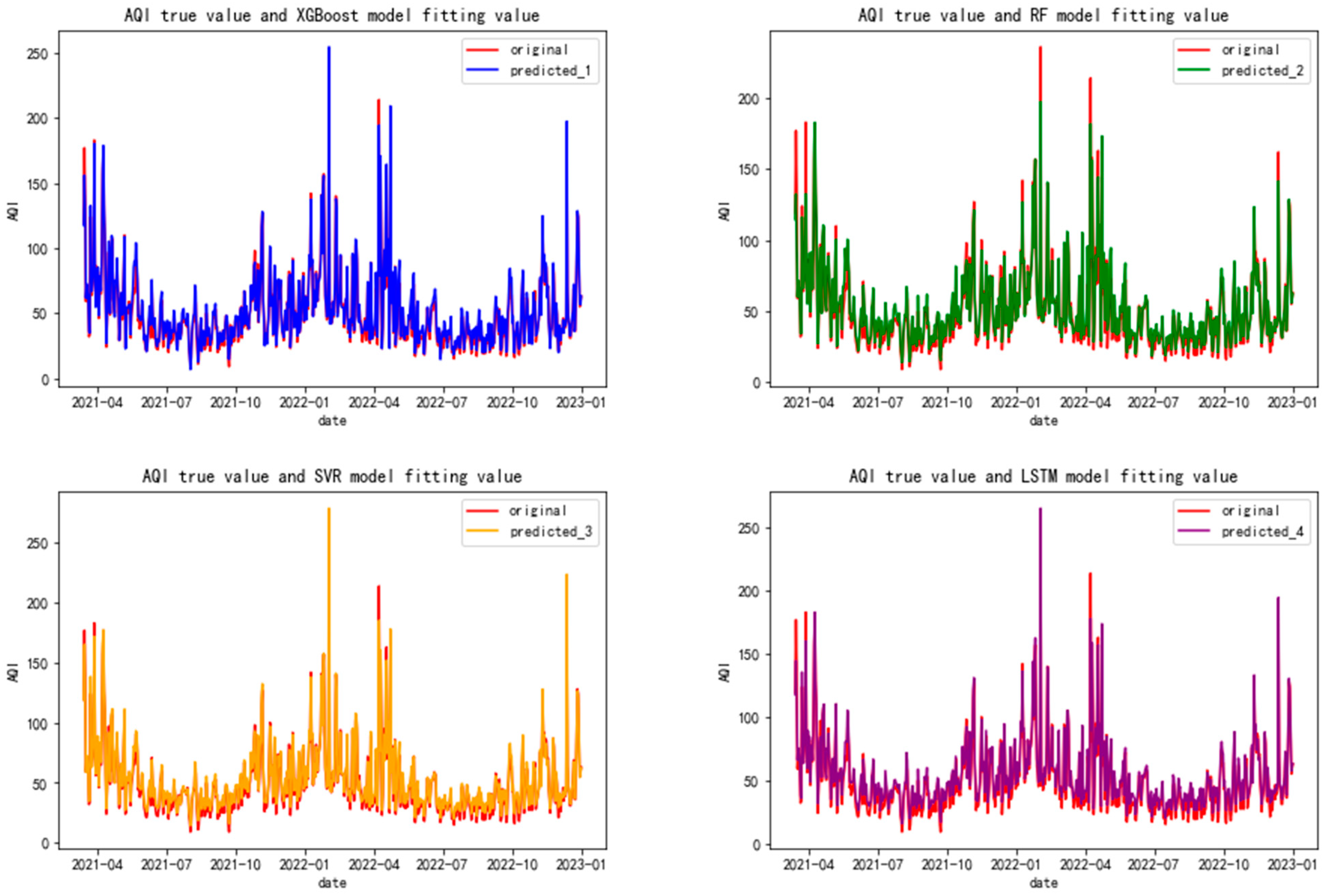
Figure 4 shows the comparison between the fitting value of the test set of the dataset without feature selection in each single model and the true value of the Changchun air quality index. In Figure 4, the red curve represents the true value of the Changchun air quality index, the green curve represents the fitting value of the test set trained using the random forest model, the yellow curve represents the fitting value of the test set trained via the SVR model, and the purple curve represents the fitting value of the test set trained using the LSTM model. It can be seen from Figure 4 that after the dataset without feature selection is trained using the SVR model, LSTM model, XGBoost model, and random forest model, the curve composed of the test set values basically coincides with the curve composed of the real value of the Changchun air quality index, indicating that the single model selected in this paper can better train and fit the data.
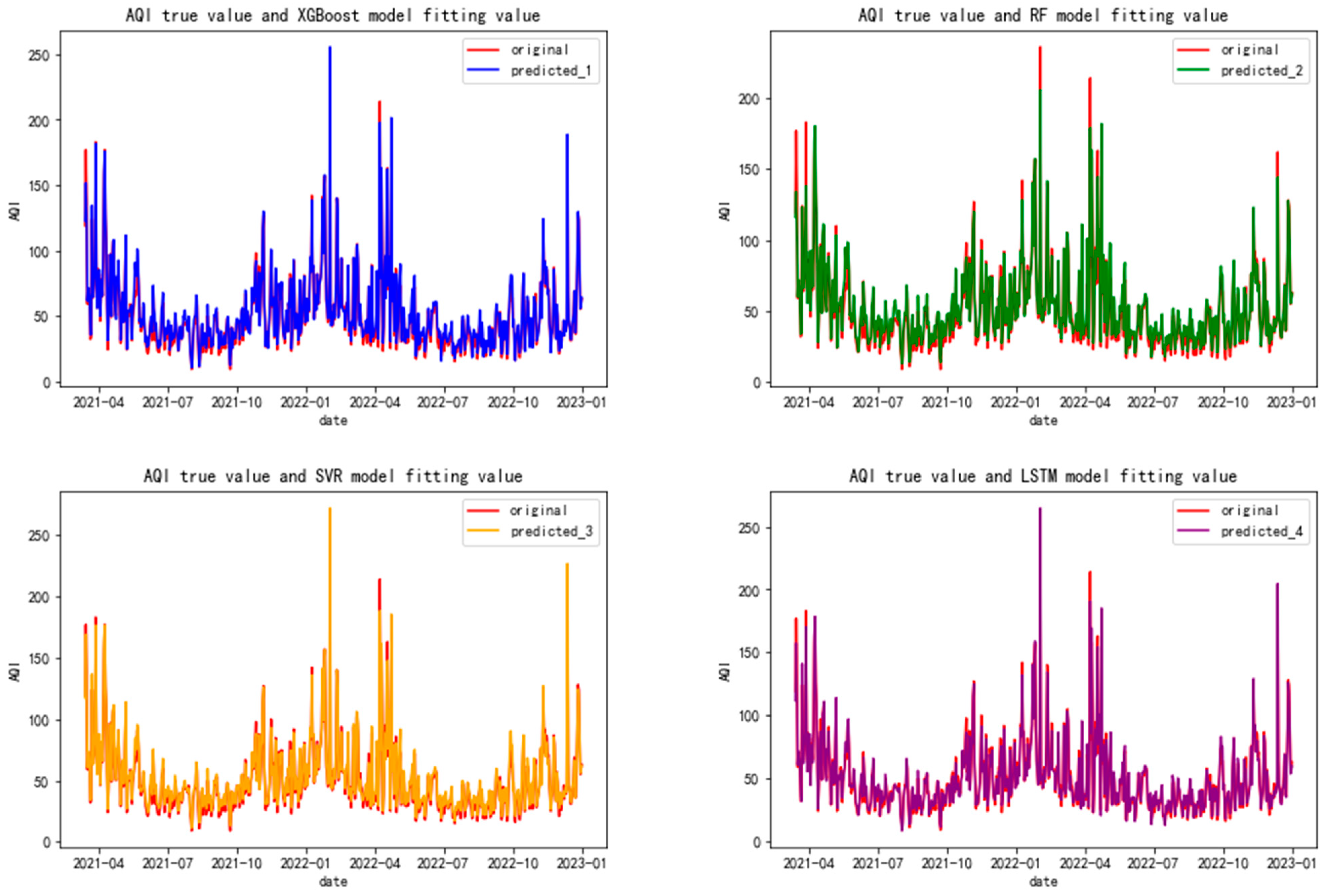
Figure 5 shows the comparison between the fitting value of the test set of the feature-selected dataset in each single model and the true value of the Changchun air quality index. In Figure 5, the red curve represents the true value of the Changchun air quality index, the green curve represents the fitting value of the test set trained using the random forest model, the yellow curve represents the fitting value of the test set trained via the SVR model, and the purple curve represents the fitting value of the test set trained using the LSTM model. As can be seen from Figure 5, after the dataset after feature selection is trained using the SVR model, LSTM model, XGBoost model, and random forest model, the curve composed of test set values basically coincides with the curve composed of the real value of the Changchun air quality index, which preliminarily shows that the dataset after feature selection using the Pearson-MI method has a good fitting effect after being trained by four single models.
Figure 4 and Figure 5 show the comparison between the fitting values of the test sets in each model and the real values of the Changchun air quality index of all datasets without feature selection and some datasets after feature selection, respectively. Table 5 shows the prediction accuracy of different datasets according to the evaluation indices.
Table 5 shows the fitting effects of the SVR model, LSTM model, XGBoost model, and random forest model on the test set. The evaluation indices include root mean square error and average absolute error to reflect the feature selection effect. It can be seen from Table 5 that when the LSTM model and XGBoost model are used to fit the data, the fitting effect of the dataset after feature selection is obviously improved compared with the dataset without feature selection. When using the SVR model and random forest model to fit the data, we can see that the fitting effect of the dataset after feature selection is not significantly improved compared with the dataset without feature selection, but it does not make the fitting effect worse, indicating that using fewer datasets can obtain the same fitting effect as using all datasets. To sum up, the feature selection method used in this paper achieves the purpose of removing redundant features, reducing computational costs, and obtaining a higher learning accuracy.

3.4. Combination Model Prediction

In order to improve the prediction accuracy of the model, this paper uses the reciprocal variance method to combine a single model to form a new combined model. Whether the combined model has a better prediction accuracy than the single model can be judged by comparing the prediction accuracy of the combined model with that of the single model. The combined model composed by the reciprocal variance method is composed by providing different weights to a single model test set, and the weights are obtained from the verification dataset, so only the predicted values composed by a single model test set through the reciprocal variance method exist in the combined model.
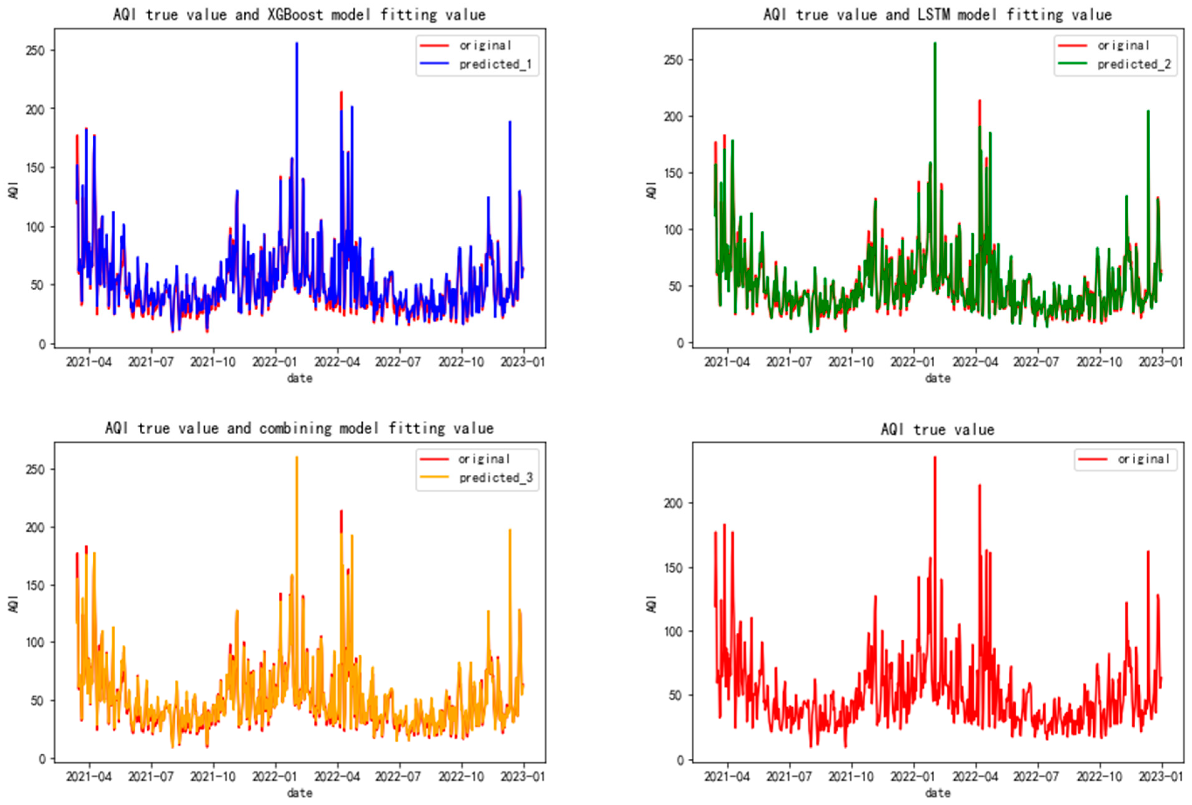
Figure 6 shows the comparison between the true value of the Changchun air quality index and the fitting value of the XGBoost model test set, the comparison between the true value of the Changchun air quality index and the fitting value of the LSTM model test set, the comparison between the true value of the Changchun air quality index and the predicted value of the combined model (composed of XGBoost model and LSTM model), and the true value of the Changchun air quality index. As can be seen from Figure 6, the LSTM model, XGBoost model, and combined model (composed of XGBoost model and LSTM model) have a good fitting effect.
Table 6 shows the evaluation indices of the LSTM model, XGBoost model test set fitting value, and the combined model (composed of XGBoost model and LSTM model) prediction value. From Table 6, it can be seen that the root mean square error and average absolute error of the LSTM model in a single model are smaller than the XGBoost model, indicating that the LSTM model has a better fitting effect than the XGBoost model and the combined model composed of the LSTM model and XGBoost model has a better prediction accuracy than two single models.
Table 7 shows the prediction accuracy of the predicted values obtained by combining different single models by the reciprocal variance method, and the number of single models used in the combined model includes two, three and four; that is, multiple single models form a combined model via the reciprocal variance method. It can be seen from Table 7 that the predicted values obtained using the LSTM model and XGBoost model through the reciprocal variance method have a higher prediction accuracy than other combined models, and the predicted values obtained by the SVR model and random forest model via the reciprocal variance method have the worst prediction accuracy compared with other combined models. It can be seen from Table 5 that the LSTM model and XGBoost model have higher fitting accuracy compared with other single models, indicating that the combined model composed of single models with a better prediction accuracy still has a higher prediction accuracy. It can also be seen from Table 7 that the increase in the number of single models used in combined models cannot improve the prediction accuracy of combined models.
To sum up, the LSTM model and XGBoost model have good fitting effects in a single model, and the combined model composed of the LSTM model and XGBoost model via the reciprocal variance method also has a good fitting effect. Therefore, when the models are combined by the reciprocal variance method, the models with a better fitting effect should be selected for combination. Meanwhile, it should be noted that there is no absolute relationship between the increase in the number of single models used in combination and the improvement in the prediction accuracy of the models.

3.5. Modified Combination Model Prediction

In order to further improve the prediction accuracy of the model and to verify the fitting effect of the modified reciprocal variance method proposed in this paper, this paper selects two models with a better fitting effect as the baseline models in the SVR model, random forest model, XGBoost model, and LSTM model, and we take the remaining two models as modified models to construct a combined model through the modified reciprocal variance method. At the same time, comparing the prediction accuracy of the modified combined models under different correction ratios, it can be seen from Table 8 that the LSTM model and XGBoost can be used as the baseline models, and the SVR model and random forest model are the modified models. Compared with the original reciprocal variance method, the modified reciprocal variance method further considers the influence of extreme values in the fitted values of the baseline model on the fitted results.
As can be seen from Figure 7, the root mean square error of the modified combined model of the LSTM model and XGBoost model via the modified reciprocal variance method shows an upward trend with the increase in the correction ratio. According to the modified reciprocal variance method, before modifying the combined model composed of the reference models, the absolute error between the two reference models is first calculated, and according to the absolute error, the fitting values of the test sets of the reference model are sorted according to the order from large to small, and then whether the fitting values of the reference model and the modified model test sets meet the modification rules of the modified reciprocal variance method is judged. If so, the fitting values of the Changchun air quality index can be modified according to the modified reciprocal variance method to make it have better accuracy, and with the continuous improvement in the modification ratio, the absolute error between the reference models will decrease, which means that the probability of the extreme deviation value will decrease. At this time, the probability of error when correcting the fitting value of the baseline model test set by correcting the fitting value of the model test set also increases, so the following situation, outlined in Figure 7, appears: with the continuous increase in the correction ratio, the root mean square error also shows an upward trend.
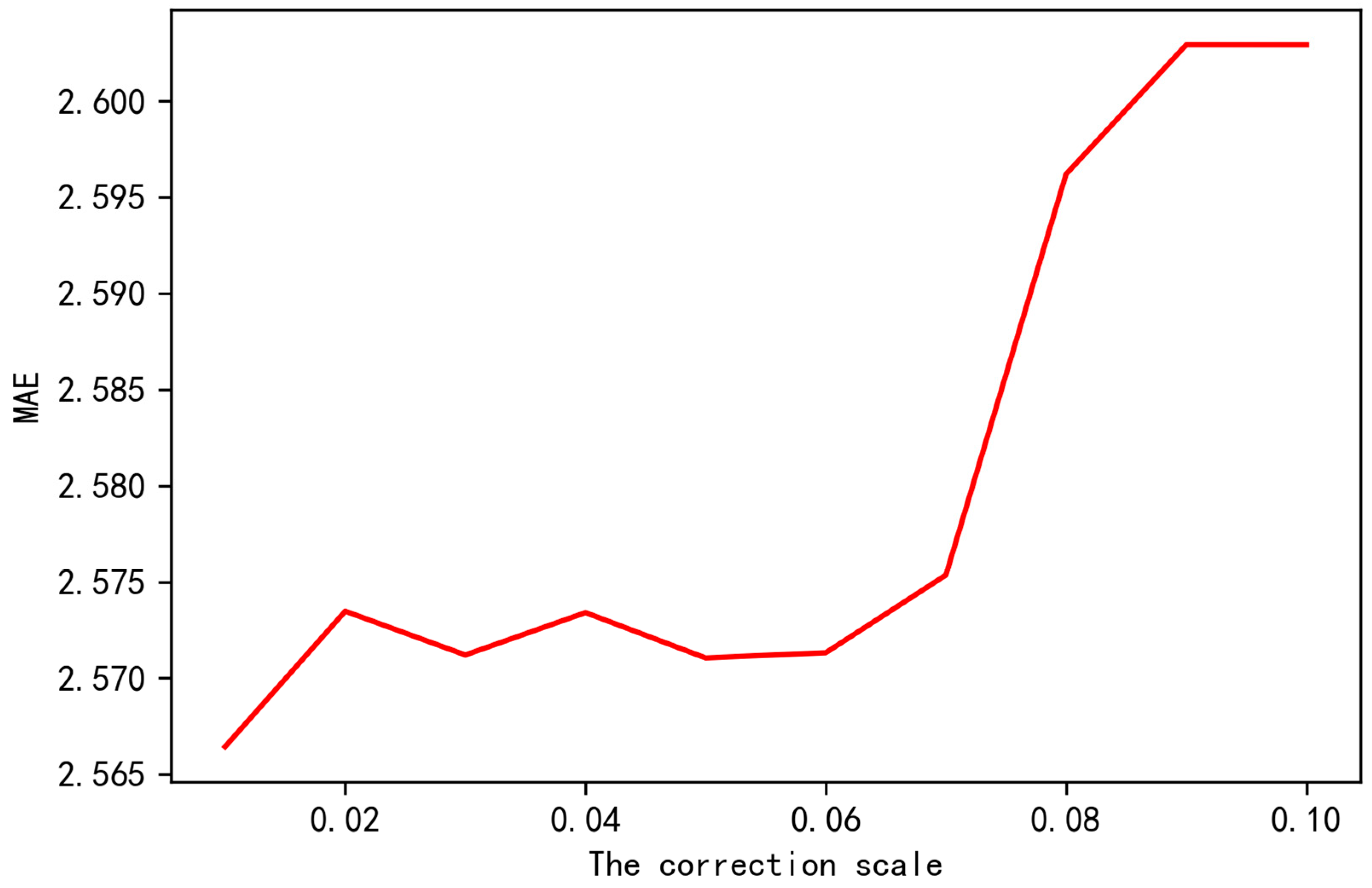
As can be seen from Figure 8, the average absolute error of the modified combined model composed of the LSTM model and XGBoost model via the modified reciprocal variance method shows an upward trend with the increase in the correction ratio. Similar to the conclusion in Figure 7, with the continuous increase in the correction ratio, the absolute error between baseline models decreases, which means that the probability of an extreme deviation value decreases. At this time, the probability of error when correcting the fitting value of the baseline model test set by correcting the fitting value of the model test set also increases, so the situation outlined in Figure 8 appears: with the continuous increase in the correction ratio, the average absolute error also shows an upward trend.
It can be seen from Figure 7 and Figure 8 that when the correction ratio is from 1% to 10%, the root mean square error and the average absolute error also show an upward trend with the continuous increase in the correction ratio. When the correction ratio is 1%, both the root mean square error and the average absolute error can reach the minimum.
Table 8 shows the prediction accuracy of the modified combined model composed of the LSTM model and XGBoost model as the baseline model, SVR model, and random forest model as the modified model and the modified reciprocal variance method under different modified ratios. It can be seen from Table 8 that the root mean square error and average absolute error of the combined model composed of the LSTM model and XGBoost model via the reciprocal variance method are 4.131 and 2.581, respectively. When the correction ratio is 8%, the average absolute error of the modified combined model is 2.596, and with continuous improvement in the correction ratio, the average absolute error of the modified combined model reaches 2.603. Therefore, it can be obtained that the modified combined model composed of the LSTM model and XGBoost model via the reciprocal variance method can improve the fitting accuracy when the correction ratio is from 1% to 7% and when the correction ratio is from 8% to 10%, although the average absolute error of the modified combined model is slightly higher than that of the combined model (composed of the LSTM model and XGBoost model via the reciprocal variance method). However, the root mean square error of the modified combined model is still better than that of the combined model. To sum up, the modified reciprocal variance method can effectively improve the prediction accuracy of the model.
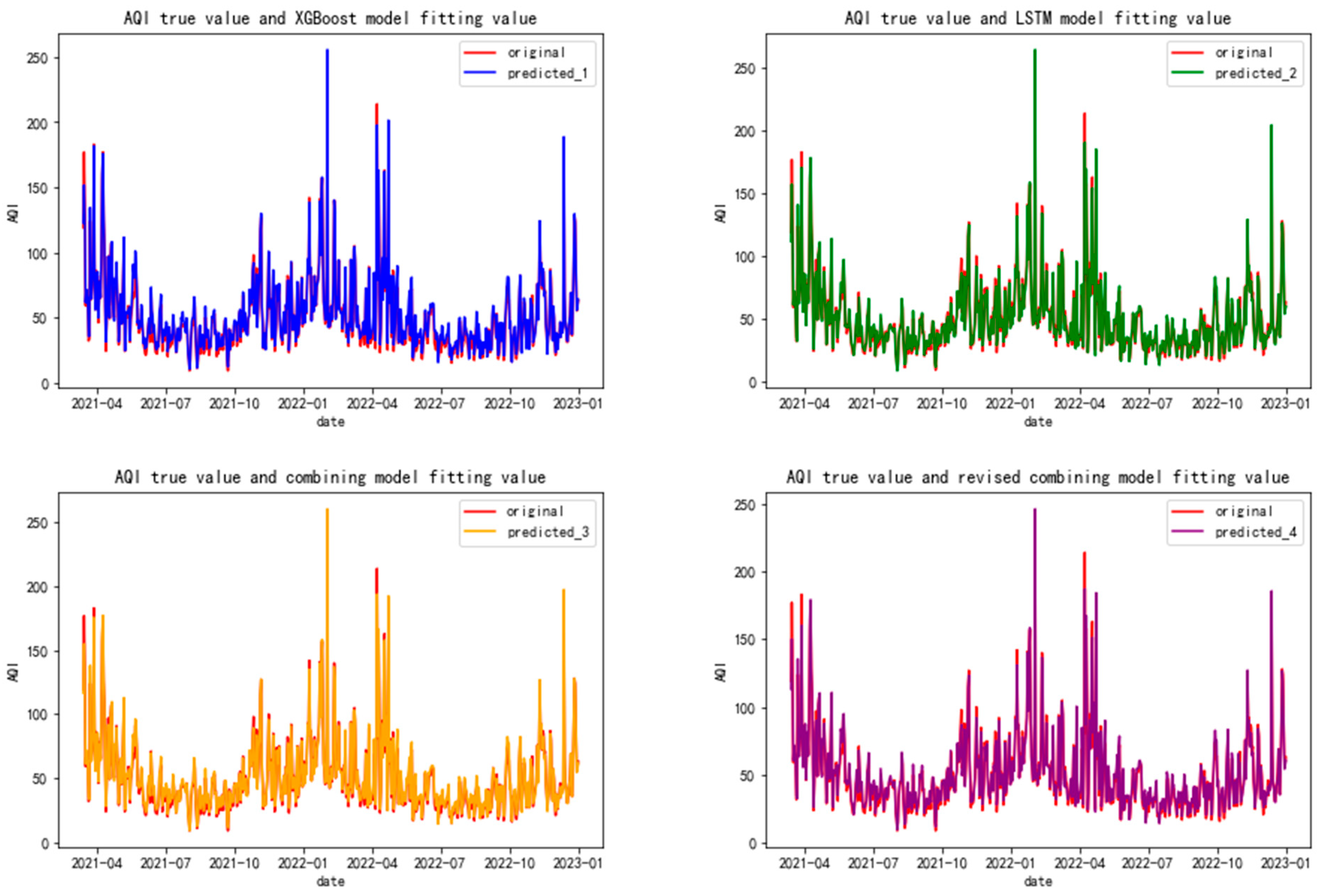
Figure 9 shows the comparison charts of the Changchun air quality index true value and XGBoost model test set, the Changchun air quality index true value and LSTM model test set, the Changchun air quality index true value and combined model (composed of XGBoost model and LSTM model) predicted value, and the Changchun air quality index true value and modified combined model (composed of XGBoost model and LSTM model) predicted value. From Figure 9, it can be seen that the LSTM model, XGBoost model, combined model, and modified combined model all have a good fitting effect.
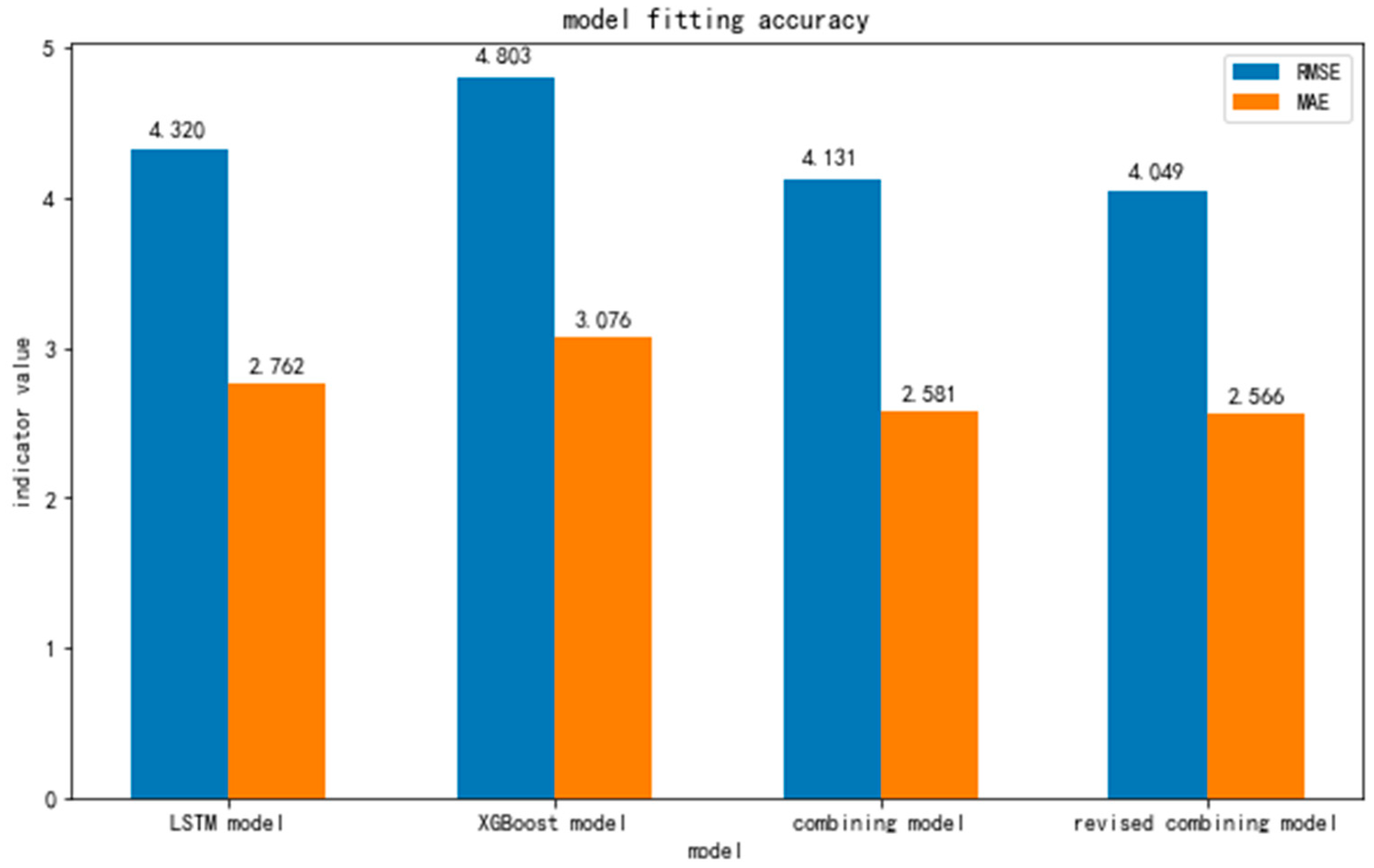
Figure 9 shows the RMSE and MAE for the different models, where the modified combined model uses a correction ratio of 1%. As can be seen from Figure 10, the combined model composed of the reciprocal variance method of the LSTM model and XGBoost model has a better prediction accuracy than the LSTM model and XGBoost model, and the modified combined model composed of the modified reciprocal variance method has a better prediction accuracy. Therefore, it can be concluded that the modified inverse variance method can effectively improve the prediction accuracy of the model under the condition that the correction proportion is 1%. To sum up, the modified inverse variance method proposed in this paper has a good effect.
4. Conclusions

In summary, this paper proposes the Pearson-MI feature selection method and the modified inverse variance method. The Pearson-MI method overcomes the nonlinear relationship between influencing factors that the Pearson correlation coefficient cannot measure, and mutual information cannot directly select influencing factors according to the value. The modified inverse variance method overcomes the influence of extreme deviation in the fitting data on the prediction results. Taking Changchun City as an example, this paper selected the factors affecting the AQI of Changchun City using the Pearson-MI method and compared the results with those obtained without the use of feature selection. The results show that the Pearson-MI method has a significant effect on improving the prediction accuracy of the model. The models used in this paper include the LSTM model, XGBoost model, SVR model, and RF model; for the selected factors affecting the air quality index of Changchun City, this study constructed a combined model using the inverse variance method, which has a better prediction accuracy than the LSTM, XGBoost, SVR, and RF models. In order to further improve the prediction accuracy of the model, in this study, the modified combination model was constructed by the modified inverse variance method. Compared with the combined model, the modified combination model reduces the RMSE by 2% and MAE by 0.6%. Therefore, the Pearson-MI method and the modified inverse variance method have great significance for the selection of the influencing factors of AQI and the improvement in the prediction accuracy of the model.

Author Contributions

F.C.: conceptualization, methodology, and writing—reviewing and editing. L.W.: data curation, writing—original draft preparation, and software. H.D.: validation, writing—reviewing and editing. All authors have read and agreed to the published version of the manuscript.

Funding

This work is supported by the National Natural Science Foundation of China (grant No. 11701077) and the Natural Science Foundation of Jilin Province (grant No. 20220101026JC, 20220201160GX, 20210101476JC).

Institutional Review Board Statement

Not applicable.

Informed Consent Statement

Not applicable.

Data Availability Statement

The data that support the findings of this study are available from the corresponding author upon reasonable request.

Conflicts of Interest

The authors declare that there are no conflicts of interest regarding the publication of this paper.

References

  1. Wang, K.; Fan, X.; Yang, X.; Zhou, Z. An AQI decomposition ensemble model based on SSA-LSTM using improved AMSSA-VMD decomposition reconstruction technique. Environ. Res. 2023, 232, 116365. [Google Scholar] [CrossRef] [PubMed]
  2. Kaur, J.; Singh, S.; Parmar, K.S. Forecasting of AQI (PM2.5) for the three most polluted cities in India during COVID-19 by hybrid Daubechies discrete wavelet decomposition and autoregressive (Db-DWD-ARIMA) model. Environ. Sci. Pollut. Res. Int. 2023. [Google Scholar] [CrossRef] [PubMed]
  3. Wang, Y.; Ding, D.; Ji, X.; Zhang, X.; Zhou, P.; Dou, Y.; Dan, M.; Shu, M. Construction of Multipollutant Air Quality Health Index and Susceptibility Analysis Based on Mortality Risk in Beijing, China. Atmosphere 2022, 13, 1370. [Google Scholar] [CrossRef]
  4. Liu, X.; Wang, P. Population Agglomeration, Air Pollution, and Economic Sustainable Development: A Spatial Econometric Analysis Based on 266 Chinese Cities at Prefecture Level and Above. Sci. Decis. Mak. 2022, 11, 81–93. (In Chinese) [Google Scholar]
  5. Chen, S.X. Scientific statistics supporting atmospheric governance. China Econ. Rep. 2017, 2017, 54–56. (In Chinese) [Google Scholar]
  6. Zhen, Q. Quantitative Identification of Urban Functional Areas in Downtown Area of Changchun Based on POI Data. In IOP Conference Series: Earth and Environmental Science; IOP Publishing: Bristol, UK, 2019; Volume 330, p. 052001. [Google Scholar]
  7. Xingpo, L.; Hongyuan, G. Air quality indicators and AQI prediction coupling long-short term memory (LSTM) and sparrow search algorithm (SSA): A case study of Shanghai. Atmos. Pollut. Res. 2022, 13, 101551. [Google Scholar]
  8. Sarkar, N.; Gupta, R.; Keserwani, P.K.; Govil, M.C. Air Quality Index prediction using an effective hybrid deep learning model. Environ. Pollut. 2022, 315, 120404. [Google Scholar] [CrossRef]
  9. Wong, Y.J.; Shiu, H.Y.; Chang, J.H.H.; Ooi, M.C.G.; Li, H.H.; Homma, R.; Shimizu, Y.; Chiueh, P.T.; Maneechot, L.; Sulaiman, N.M.N. Spatiotemporal impact of COVID-19 on Taiwan air quality in the absence of a lockdown: Influence of urban public transportation use and meteorological conditions. J. Clean. Prod. 2023, 365, 132893. [Google Scholar] [CrossRef]
  10. Zhao, B.; Wong, Y.; Ihara, M.; Nakada, N.; Yu, Z.; Sugie, Y.; Miao, J.; Tanaka, H.; Guan, Y. Characterization of nitrosamines and nitrosamine precursors as non-point source pollutants during heavy rainfall events in an urban water environment. J. Hazard. Mater. 2022, 424, 127552. [Google Scholar] [CrossRef]
  11. Rakholia, R.; Le, Q.; Vu, K.; Ho, B.Q.; Carbajo, R.S. AI-based air quality PM2.5 forecasting models for developing countries: A case study of Ho Chi Minh City, Vietnam. Urban Clim. 2022, 46, 101315. [Google Scholar] [CrossRef]
  12. Luo, S.; Zhu, Y.; Chen, S.X. Episode based air quality assessment. Atmos. Environ. 2022, 285, 119242. [Google Scholar] [CrossRef]
  13. Zhang, X.; Lin, M. Regional disparities of urban air pollution in China and analysis of socio-economic influencing factors: A comparative study based on two air quality indices. J. Univ. Chin. Acad. Sci. 2020, 37, 39–50. (In Chinese) [Google Scholar]
  14. Zhao, Y.; Zhang, X.; Chen, M.; Gao, S.; Li, R. Regional disparities and attribution analysis of urban air quality in China. Acta Geogr. Sin. 2021, 76, 2814–2829. (In Chinese) [Google Scholar]
  15. Bouke, M.A.; Abdullah, A.; ALshatebi, S.H.; Abdullah, M.T.; El Atigh, H. An intelligent DDoS attack detection tree-based model using Gini index feature selection method. Microprocess. Microsyst. 2023, 98, 104823. [Google Scholar] [CrossRef]
  16. Guendouz, M.; Amine, A. A New Wrapper-Based Feature Selection Technique with Fireworks Algorithm for Android Malware Detection. Int. J. Softw. Sci. Comput. Intell. (IJSSCI) 2022, 14, 1–19. [Google Scholar] [CrossRef]
  17. Sethi, J.K.; Mittal, M. An efficient correlation based adaptive LASSO regression method for air quality index prediction. Earth Sci. Inform. 2021, 14, 1777–1786. [Google Scholar] [CrossRef]
  18. Maltare, N.N.; Vahora, S. Air Quality Index prediction using machine learning for Ahmedabad city. Digit. Chem. Eng. 2023, 7, 100093. [Google Scholar] [CrossRef]
  19. Shi, K.; Ding, R.; Wu, L.; Zheng, Y. Construction of a New Grey System Multiple Model for Predicting Air Quality—A Case Study of Shijiahua City. Chinese J. Syst. Sci. 2023, 2, 75–81. [Google Scholar]
  20. Singh, T.; Sharma, N.; Satakshi; Kumar, M. Analysis and forecasting of air quality index based on satellite data. Inhal. Toxicol. 2023, 35, 24–39. [Google Scholar] [CrossRef]
  21. Wong, Y.J.; Yeganeh, A.; Chia, M.Y.; Shiu, H.Y.; Ooi, M.C.G.; Chang, J.H.W.; Shimizu, Y.; Ryosuke, H.; Try, S.; Elbeltagi, A. Quantification of COVID-19 impacts on NO2 and O3: Systematic model selection and hyperparameter optimization on AI-based meteorological-normalization methods. Atmos. Environ. 2023, 301, 119677. [Google Scholar] [CrossRef]
  22. Xu, T.; Yan, H.; Bai, Y. Air pollutant analysis and AQI prediction based on GRA and improved SOA-SVR by considering COVID-19. Atmosphere 2021, 12, 336. [Google Scholar] [CrossRef]
  23. Phruksahiran, N. Improvement of air quality index prediction using geographically weighted predictor methodology. Urban Clim. 2021, 38, 100890. [Google Scholar] [CrossRef]
  24. Yan, R.; Liao, J.; Yang, J.; Sun, W.; Nong, M.; Li, F. Multi-hour and multi-site air quality index forecasting in Beijing using CNN, LSTM, CNN-LSTM, and spatiotemporal clustering. Expert Syst. Appl. 2021, 169, 114513. [Google Scholar] [CrossRef]
  25. Khan, M.A.; Zafar, A.; Farooq, F.; Javed, M.F.; Alyousef, R.; Alabduljabbar, H.; Khan, M.I. Geopolymer concrete compressive strength via artificial neural network, adaptive neuro fuzzy interface system, and gene expression programming with K-fold cross validation. Front. Mater. 2021, 8, 621163. [Google Scholar] [CrossRef]
  26. Bigoni, C.; Cadic-Melchior, A.; Morishita, T.; Hummel, F.C. Optimization of phase prediction for brain-state dependent stimulation: A grid-search approach. J. Neural Eng. 2023, 20, 016039. [Google Scholar] [CrossRef] [PubMed]
Figure 1. Overall framework.
Atmosphere 14 01475 g001
Figure 2. Feature selection flow chart of Pearson-MI method.
Atmosphere 14 01475 g002
Figure 3. Flow chart of revised combined model.
Atmosphere 14 01475 g003
Figure 4. Comparison of fitting effect between AQI true value and single model test set (all data).
Atmosphere 14 01475 g004
Figure 5. Comparison of fitting effect between AQI true value and single model test set (partial dataset).
Atmosphere 14 01475 g005
Figure 6. Comparison of fitting effect of LSTM model, XGBoost model, and corresponding combination model.
Atmosphere 14 01475 g006
Figure 7. Root mean square error of modified combined model under different correction ratios.
Atmosphere 14 01475 g007
Figure 8. Average absolute error of modified combined model under different correction ratios.
Atmosphere 14 01475 g008
Figure 9. Comparison of fitting effect of LSTM model, XGBoost model, corresponding combination model, and modified combination model.
Atmosphere 14 01475 g009
Figure 10. Fitting accuracy of LSTM model, XGBoost model, and combined model.
Atmosphere 14 01475 g010
Table 1. Air quality index and corresponding grades.
Air Quality IndexAir Quality Index LevelAir Quality Index Category
0–50Level 1Excellent
51–100Level 2Good
101–150Level 3Mild Pollution
151–200Level 4Moderate Pollution
201–300Level 5Heavy Pollution
>300Level 6Serious Pollution
Table 2. Mutual information between AQI and influencing factors and Pearson correlation coefficient.
IndicatorsMIPearson Correlation Coefficient
Gas prices 3.8630.220
Minimum temperature 3.486−0.021
Average temperature 3.456−0.021
Maximum temperature 3.439−0.021
Average pressure 3.195−0.020
AQI ranking on the day 3.1160.586
NO2 2.9230.689
Minimum air pressure 2.8890.254
Maximum air pressure 2.8720.291
SO2 2.6290.524
Average relative humidity 2.507−0.021
PM2.5 2.3170.946
Maximum wind speed 2.044−0.032
O3 1.8180.043
PM10 1.7000.936
CO 1.6750.777
Minimum relative humidity 1.596−0.148
Maximum wind speed 1.5530.005
Daily precipitation 0.973−0.012
Natural gas prices0.2330.232
Table 3. Mutual information and linear correlation number among influencing factors.
Influencing factorsAverage MINumber of Linear Correlations
Minimum temperature 3.3803
Average temperature 3.3584
Maximum temperature 3.3423
Average pressure 3.1384
Minimum air pressure 2.8741
Maximum air pressure 2.8581
Average relative humidity 2.5454
PM10 concentration 2.4841
CO concentration 2.2921
PM2.5 concentration2.2192
Table 4. Minimum redundancy of each influencing factor combination.
Number of Influencing FactorsMinimum Redundancy
82.743
92.664
102.620
112.624
122.617
Table 5. Comparison of feature selection effects.
ModelRoot Mean Square ErrorThe Average Absolute Error
SVR (full data)5.2103.520
SVR (feature selection)5.2473.370
LSTM (all data)5.8894.715
LSTM (feature selection)4.3202.762
XGBoost (all data)5.0393.241
XGBoost (feature selection)4.8033.076
Random forest (full data)6.3954.181
Random forest (feature selection)6.3724.190
Table 6. Evaluation indices of prediction effect of LSTM model, XGBoost model, and corresponding combination model.
ModelRoot Mean Square ErrorThe Average Absolute Error
LSTM (feature selection)4.3202.762
XGBoost (feature selection)4.8033.076
LSTM, XGBoost4.1312.581
Table 7. Effect of combined model based on reciprocal variance method.
ModelRoot Mean Square ErrorThe Average Absolute Error
LSTM, XGBoost4.1312.581
LSTM, SVR4.5062.813
LSTM, random forest4.2962.835
SVR, random forest5.0133.529
SVR, XGBoost4.7123.022
XGBoost, random forest4.8843.240
SVR, XGBoost, random forest4.6993.186
SVR, XGBoost, LSTM4.3242.691
SVR, random forest, LSTM4.4152.906
XGBoost, random forest, LSTM4.2092.723
SVR, XGBoost, random forest, LSTM4.3232.803
Table 8. Fitting accuracy of combined models with different correction ratios.
Correction RatioRoot Mean Square ErrorThe Average Absolute Error
1%4.0492.566
2%4.0502.573
3%4.0512.571
4%4.0522.573
5%4.0592.571
6%4.0572.571
7%4.0632.575
8%4.0922.596
9%4.0942.603
10%4.0912.603
Disclaimer/Publisher’s Note: The statements, opinions and data contained in all publications are solely those of the individual author(s) and contributor(s) and not of MDPI and/or the editor(s). MDPI and/or the editor(s) disclaim responsibility for any injury to people or property resulting from any ideas, methods, instructions or products referred to in the content.