Seasonal Changes in Atmospheric Optical Turbulence in a Near Maritime Environment Using Turbulence Flux Measurements

Abstract

Light propagation through the atmosphere is affected by fluctuations in the refractive index along the path of propagation, called optical turbulence. In the atmospheric surface layer, these fluctuations are due mostly to turbulent mixing of variations in temperature. To this end, a characterization of the atmospheric surface layer above the water in Maryland, USA, is presented. Meteorological data were collected from a sensor array comprising two sonic anemometers and an infrared gas analyzer (IRGASON) over the 12-month period from January to December, 2021. The instruments were positioned vertically at heights of approximately 4 m, 6 m, and 8 m above the water. The temperature structure parameter $C_T^2$ was calculated and scaled using Monin–Obukhov assumptions. We find that the distribution of atmospheric stability presents as an approximately normal distribution during the winter and early spring, but is skewed negatively during the summer and late fall. We hypothesize that this could be due to a more stable stratification of the underlying water during summer months. Under unstable (−z/L) conditions, turbulent quantities including the temperature structure parameter scale in a manner consistent with the literature, but with generally better agreement during the summer months. Additionally, the $C_T^2$ estimations appear more consistent during the summer months across all values of (z/L). Under stable (+z/L) conditions, there are wide variations in $C_T^2$, which is also consistent with the literature.

1. Introduction

Atmospheric optical transmission is a primary interest for the scientific community due to its wide range of applications. Technologies in the areas of directed energy, remote sensing, target designation, ranging, defensive countermeasures, and communication are of specific interest. As these optical technologies continue to develop, measurement and prediction of the major factors which impact laser systems will become increasingly important, including a deeper understanding of optical turbulence parameters. Specifically, optical turbulence can have deleterious effects on system performance due to scintillation, beam spreading, beam wander, and reduced coherence [1]. The refractive index fluctuations in the atmosphere, generally due to temperature fluctuations, must be understood to advance these laser-based technologies [2]. Near maritime (coastal, littoral) environments are frequently the site of these systems, but are not as well characterized as terrestrial or open ocean environments [3,4,5].

Measurements of optical turbulence are often accomplished using a scintillometer, which can measure path-integrated surface fluxes of sensible heat, latent heat, and momentum over large-scale, heterogeneous surfaces without flow distortion [6]. The scintillometer is a double ended method in which a transmitter and receiver are required; a setup that can be difficult to employ in certain environments and for mobile platforms. Other methods have been developed to estimate optical turbulence from macrometeorological techniques [7,8,9,10,11], or with machine learning [3,4,5]. Turbulence flux methods that make use of Monin–Obukhov Similarity Theory (MOST) may also yield direct measurements of the optical turbulence structure along with other atmospheric surface layer quantities [6,12,13,14,15,16,17,18]. In this paper, we apply turbulence flux methods to the near-maritime environment and extend the literature in an area that is not as well characterized. Specifically, we employ a sensor array consisting of two sonic anemometers and one infrared gas analyzer which were used to provide local measurements of velocity and temperature over a 12 month period during 2021.

The instruments were situated in the surface layer, which is the lowest part of the atmospheric boundary layer, and which plays a primary role in the transport of suspended particles, water vapor, and heat [12,19]. This paper seeks to explore the atmospheric surface layer in a near-maritime environment as compared to over the open ocean or over land, as the near-maritime environment tends to be markedly different in both its seasonal and diurnal variations. This project uses the MOST scaling for both stable and unstable conditions, enabling one to model the normalized variances of the wind velocity and temperature, and allowing for a global comparison of the characteristics of the atmospheric surface layer. Emphasis here is placed on scaling of the constant for the second order structure function of temperature, $C_T^2$. The temperature structure constant is the characteristic of the atmosphere that most directly affects optical propagation, and the characteristic most useful to optical engineers. Using MOST to examine $C_T^2$ scaling can provide researchers with the knowledge of how temperature and wind fluctuations in a near maritime environment will affect optical system performance.

2. Background

Calculation of $C_T^2$ typically comes from an assumed form for the second order structure function of temperature,

$$D_T\left(r\right)=\overline{{\left[T\left(x\right)-T(x+r)\right]}^2}=C_T^2{r}^{2/3}$$

(1)

where r is a streamwise separation between two points, and with the $r^{2/3}$ scaling valid over an appropriate range of scales. The structure constant $C_T^2$ then serves as a single parameter that can describe the magnitude of temperature fluctuations within a turbulent environment.

Established similarity theory may be used to scale a range of quantities within the atmospheric surface layer [13]. In the surface layer, or the constant flux layer of the atmosphere, the turbulence structure may be scaled via five parameters: a friction velocity, the surface temperature flux, the surface flux of a conserved scalar, the buoyancy parameter, and a length scale z usually taken as the height of interest. The structure parameters for temperature or refractive index, when properly non-dimensionalized, are then only functions of a non-dimensional stability parameter. This scaling within the surface layer has been used successfully in a wide range of applications [6,12,13].

In Monin–Obukhov similarity theory, velocity may be scaled with the friction velocity, $u_{\ast }$, which is related to the shear stress and defined as

$$u_{\ast }={\left[{\overline{u^{{}^{\prime }}{w}^{{}^{\prime }}}}^2+{\overline{v^{{}^{\prime }}{w}^{{}^{\prime }}}}^2\right]}^{\frac{1}{4}},$$

(2)

where $u^{{}^{\prime }}$, $v^{{}^{\prime }}$, and $w^{{}^{\prime }}$ are the fluctuating velocity components in the stream wise, transverse, and vertical directions, and where the over-bar denotes averaging. The Obukhov length scale, L, is then

$$L=-\frac{u_{\ast }^3}{k\left(\frac{g}{\overline{T}}\right)\left(\overline{w^{{}^{\prime }}T{}^{\prime }}\right)},$$

(3)

where $\overline{T}$ is the virtual air temperature in Kelvin, g is the gravitational constant, and k is the Von-Karman constant of 0.41. Nondimensionalization of temperature will use the turbulent temperature scale, $T_{\ast }$, defined as

$$T_{\ast }=-\frac{\left(\overline{w^{{}^{\prime }}{T}^{{}^{\prime }}}\right)}{u_{\ast }}.$$

(4)

Finally, using the Obukhov length and a reference height, the stability parameter $\frac{z}{L}$ is

$$\frac{z}{L}=-\frac{\left(g/\overline{T}\right)\left(\overline{w^{{}^{\prime }}{T}^{{}^{\prime }}}\right)}{u_{\ast }^3/kz},$$

(5)

where z is, for maritime measurements, the vertical height from the waterline. This stability parameter may be interpreted as a ratio of the amount of turbulence generated from buoyancy compared to the amount of turbulence generated from shear. Given these scaling parameters, MOST theory then allows the non-dimensional scaling of turbulent quantities within the surface layer as a function of just the stability parameter. For example, the turbulent velocity fluctuations ${\sigma }_i$ will scale as [12,20,21,22]

$$\frac{{\sigma }_i}{u_{\ast }}={\varphi }_i\left(\frac{z}{L}\right)=A_i{\left[1+B_i\left|\frac{z}{L}\right|\right]}^{C_i},i=u,v,w;$$

(6)

where $A_i$, $B_i$, $C_i$, are the scaling coefficients determined from field experiment. Likewise, the temperature structure constant $C_T^2$ will be non-dimensionalized and scaled as

$$\frac{{\left(kz\right)}^{2/3}{C}_T^2}{T_{\ast }^2}={\varphi }_i\left(\frac{z}{L}\right).$$

(7)

The similarity functions fitted for non-dimensional $C_T^2$ are, according to Wyngaard [13]:

$$\frac{{\left(kz\right)}^{2/3}{C}_T^2}{T_{\ast }^2}=6.7k^{2/3}{\left(1-14.9\frac{z}{L}\right)}^{-2/3}$$

(8)

and under stable conditions

$$\frac{{\left(kz\right)}^{2/3}{C}_T^2}{T_{\ast }^2}=4.5k^{2/3}\left(1+1.3{\left(\frac{z}{L}\right)}^{2/3}\right)$$

(9)

3. Experimental Setup and Data Processing

To determine the surface layer turbulence structure in the context of Monin–Obukhov Similarity Theory, eddy covariance is used with data from an array of sonic anemometers. The setup and implementation of this technique are described below.

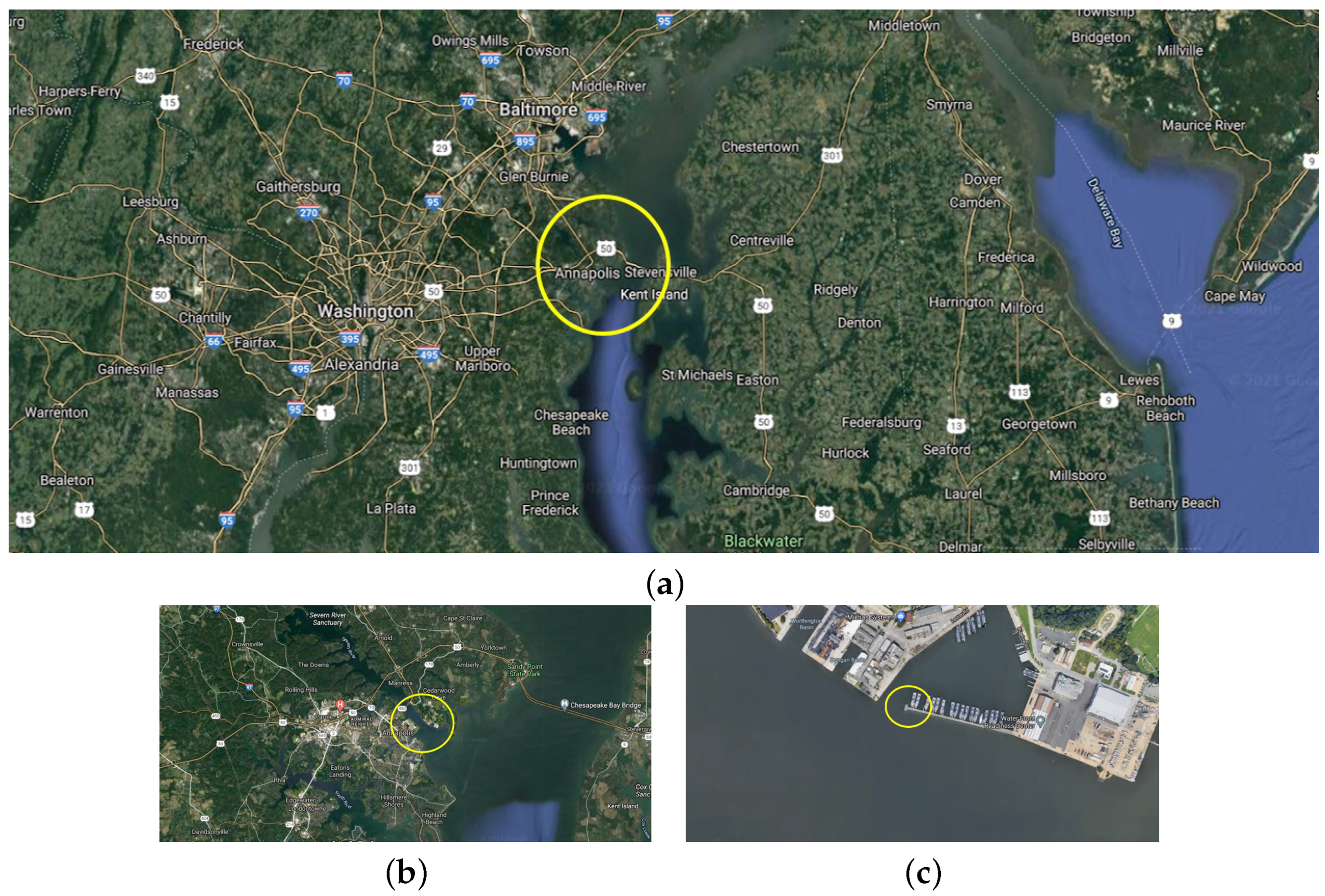
The testing location is on a pier at the U.S. Naval Academy (38.58 N, 076.28 W) in Annapolis, Maryland off the Severn River. The Severn River stems from the Chesapeake Bay which is a partially enclosed estuary located in the mid-Atlantic region of the United States and is separated from the Atlantic Ocean by the Delmarva Peninsula. Figure 1 depicts the testing location which is east of Washington D.C., and south-south east of Baltimore. The sensor array is on a 100 meter long pier and adjacent to a number of other environmental monitoring instruments which have been used previously for atmospheric optical turbulence study [3,4]. The outlying area surrounding the sensor array includes a large structure located approximately 100m to the East, several other buildings approximately 100m across the water to the North, and land masses surrounding the body of water from the east to the west with mostly open fetch of water from 090 to 270 degrees.

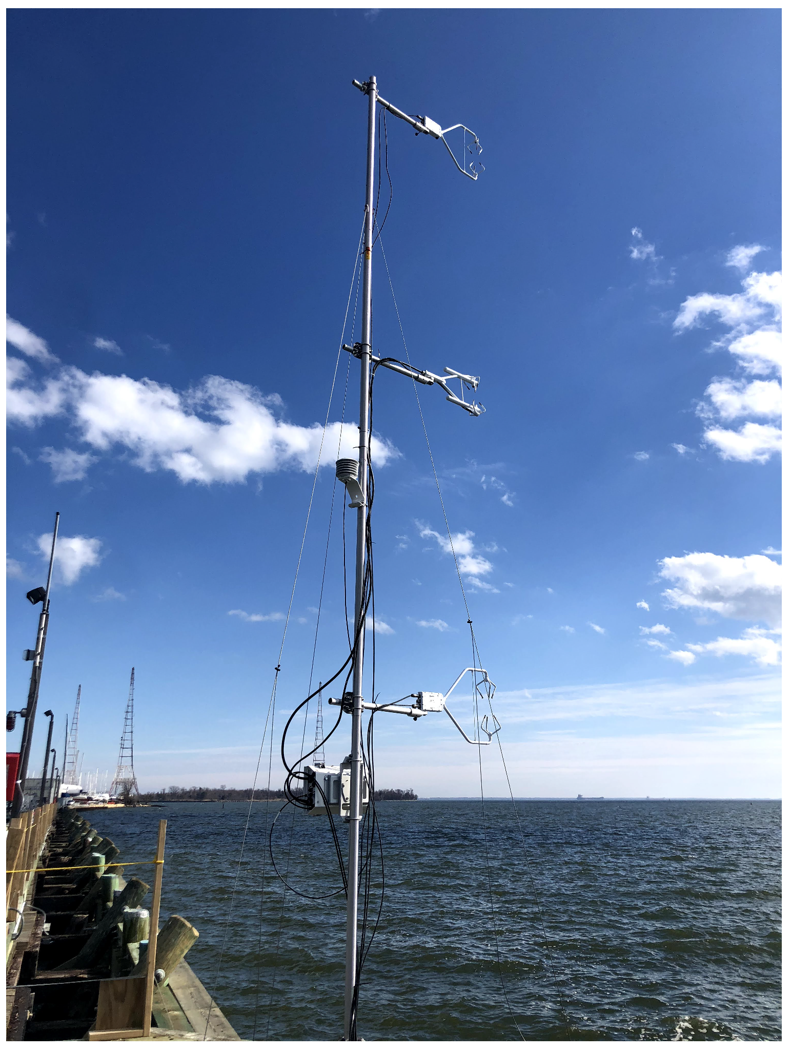
Eddy covariance measurements at this location are obtained via two Campbell Scientific CSAT3B sonic anemometers and one IRGASON infrared gas analyzer. The IRGASON is an in-situ, open-path, mid infrared absorption gas analyzer integrated with a three-dimensional sonic anemometer providing orthogonal wind components and optimized for remote eddy-covariance flux applications. Its data collection center, the EC100, measures and controls the output elements of the IRGASON such as wind velocity components, sonic air temperature, ambient temperature, $H_{2}O$ and $C{O}_2$ density. The sonic anemometer (CSAT3B) is an ultrasonic anemometer used for measuring sonic temperature and three-dimensional wind velocity. The sensor array described in this paper uses two CSAT3Bs in order to provide a more complete profile of the atmospheric surface layer above the Severn River.

All three instruments are mounted on a 6 m tall mast approximately 100 m down the pier. The mast is bolted down and supported by guy wires keeping the vertical stability within a range of $\pm 3$ degrees for any unusually high wind velocities. The two CSAT3B sonic anemometers were placed as the highest and lowest sensors with the IRGASON placed in the center of the mast due to the weight of its collection center. The mean heights of the sensors are 8, 6, and 4 m above the waterline. These heights vary with Severn River tides, which have a typical diurnal variation of approximately 1.3 m. The complete mast can be seen in Figure 2.

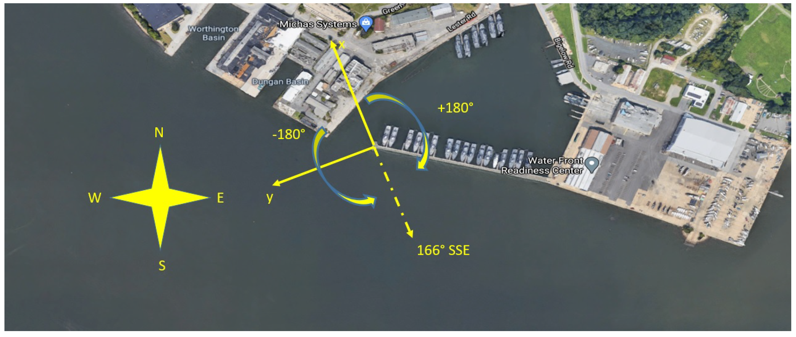
The orientation of the instruments is shown in Figure 3. The sensor array is facing 166° from true north, approximately South-South East. The positive x-axis for each sonic anemometer and IRGASON corresponds to the flow into the shaft of each instrument, therefore the u velocity component will be oriented to flow at 346°, while w is vertical. All wind velocity readings are reported as wind vectors and not meteorological wind direction. Some additional details of the instrumentation setup are outlined in reference [24].

The collection period presented here is from January 2021 to December 2021. Data are logged continuously with intermittent stops for data collection lasting roughly 30 min, and occasional outages due to power loss. The sensors were programmed to collect at 40 Hz (25 ms) intervals. Each CSAT3B sonic anemometer and IRGASON is factory calibrated and has a maximum wind accuracy offset error of less than ±8 cm·s${}^{-1}$ and a measurement resolution of 1 mm·s${}^{-1}$ rms for the stream wise and transverse wind directions. Data conditioning included double rotation [25] as well as outlier identification and linear detrending. The fluctuating components, $u^{{}^{\prime }}=u-\overline{u}$, where $\overline{u}$ is the mean from each 30 min interval, were calculated from the linearly detrended data.

The application of Monin–Obukhov theory requires a flat, horizontally homogeneous surface, with roughness length significantly less than the Obukhov length z. The statistics presented below are from data that were filtered to require mean wind velocity magnitude greater than 2 m/s and wind directions with fetch over the Chesapeake encompassing an arc of 124°. Approximately 23% of the data set met both of these criterion and was included in the statistical analysis. Preliminary statistics for each of the instruments on the tower showed that the kinetic energy from the lowest sonic anemometer, at 4 m above the water, did not scale the same as for the other two instruments. We concluded that this anemometer was subject to mechanical effects from the surface topography, but that the IRGASON and the highest anemometer were both adequately positioned within the surface layer. The data presented here are from these top two instruments, unless otherwise noted. Other environmental factors including cloud cover or solar radiation may influence results, but are not controlled for here. For simplicity, most of the monthly results below are from the odd-numbered months: January, March, May, etc., which capture the seasonal variations over the full twelve months of data.

4. Results and Discussion

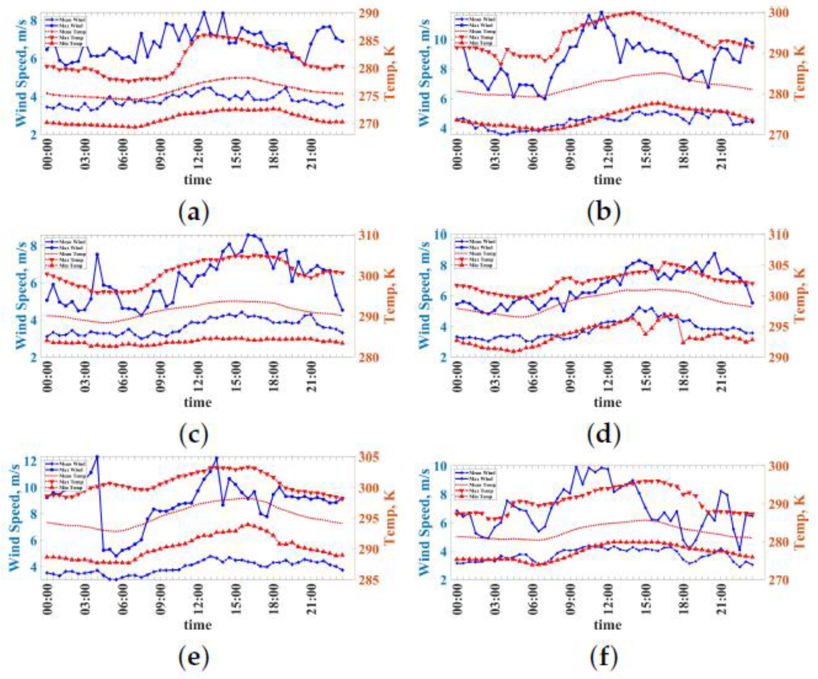
Figure 4 show the diurnal temperature and wind velocity magnitude changes throughout the year, featuring specifically the odd numbered months of January, March, May, July, September, and November. The data are from the IRGASON at a height of 6 m above the water. The minimum and maximum lines are the minimum and maximum values, respectively, for the ensemble average of that 30 min increment in the month. The mean temperature shows an increase of approximately twenty degrees from January to July. Maximum wind velocities are calculated in a similar manner as the maximum temperature. Because 30 min periods with wind velocity under 2 m/s were filtered out, minimum average wind velocities are not shown. Low wind speeds risk that the turbulence is underdeveloped, and periods of low wind speed or low turbulence intensity may not conform to Monin–Obukhov theory or to Taylor’s hypothesis [12]. From the figure, we see relatively consistent average wind speeds throughout the year, with slightly higher values in the spring and fall. Wind speeds are larger during the day than at night, but maximum values, likely coming from storms, are more randomly distributed.

Histograms of the stability parameter for March and September are shown in Figure 5. The winter and early spring months, as shown in the March histogram, show an approximately normal distribution of values, while the summer and early fall months, as in the September data, exhibit significant negative skewness. One possible explanation for this is the stronger stratification within the water during the summertime, when the surface waters of the Chesapeake receive more solar heating and there is less vertical mixing of the bay. This would contribute to higher temperatures at the bottom boundary of the atmosphere, an increased likelihood of a negative air water temperature difference, and negative stability during this time.

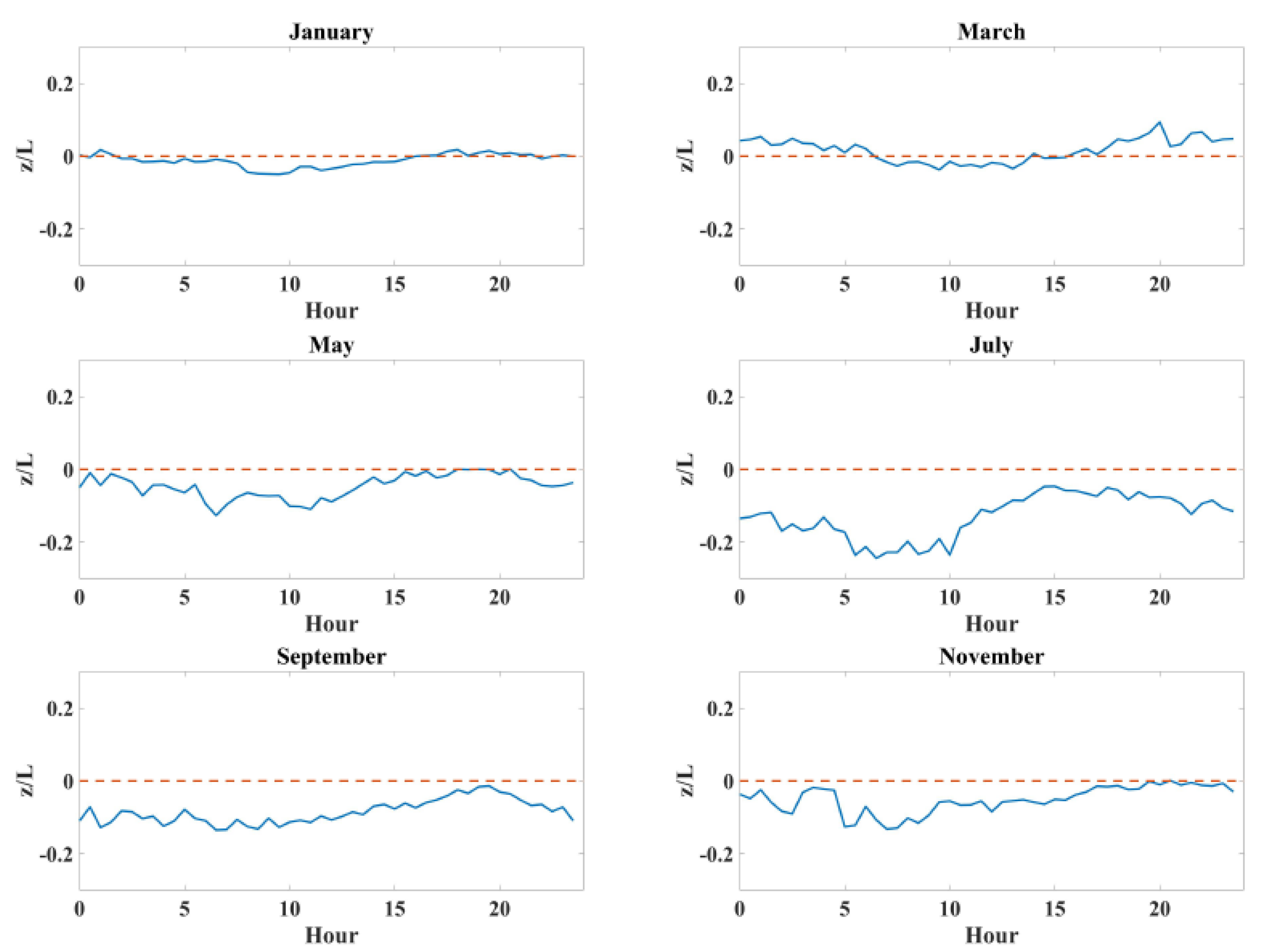
The average (median) diurnal variations in the atmospheric stability parameter, z/L are presented bi-monthly for 2021 in Figure 6. Note the small range for z/L here compared to the histogram in Figure 5; while there are significant month-to-month differences, the average for every month does not deviate far from zero (neutral stability.) Here, we see a larger peak-to-trough amplitude of variation in the summer months, even with few positive stability conditions. There are some differences in these data compared to the results from Prasad et al., which come from a coastal station in India [14]. They saw unstable conditions forming rapidly in the morning hours, and relatively few stable periods at any time of the day or year. The Chesapeake data, by contrast, only exhibits the same trends during the winter and early spring, with the March data as a representative example. In the summer and early fall, the atmosphere remains unstable through the night and has a relatively small dip correlated with sunrise. Again, a possible explanation is that the warm and stably stratified waters of the Bay continue to induce a strong vertical heat flux throughout the night even after the air temperatures, with strong terrestrial influence, have dropped.

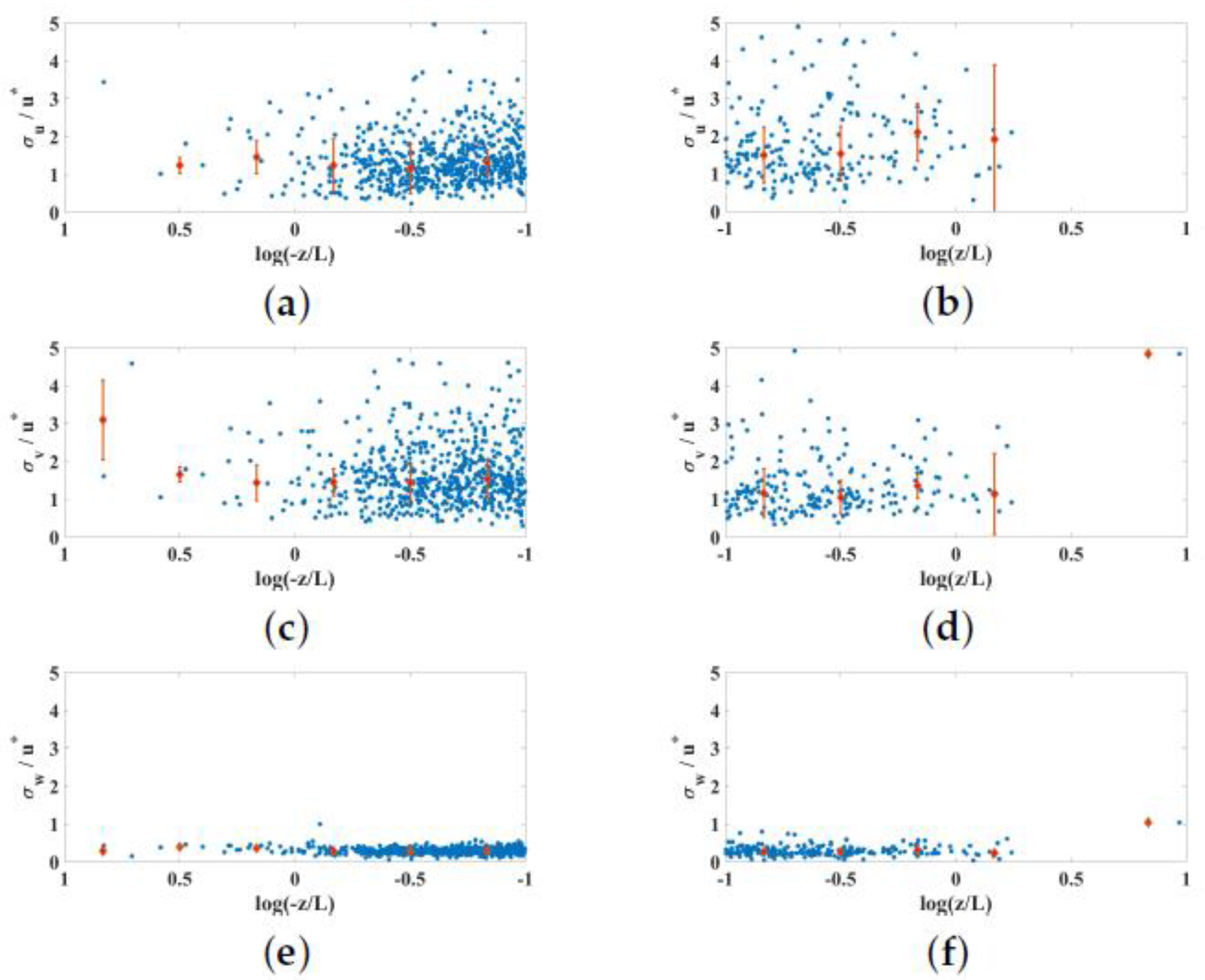
Figure 7 shows turbulent velocity fluctuations normalized by the friction velocity, ${\sigma }_i/u_{\ast }$ for both negative (left) and positive (right) stability conditions. Note the log scale on the horizontal axis such that the neutral stability case is to the far right on the negative stability plots, and to the far left on the positive stability plots. Overall, the normalized velocities for the negative stability cases match nicely with other results for the atmospheric surface layer found in the literature [12,14]. Positive stability velocity fluctuations show a reluctance to collapse, as has also been shown by many others. We see similar magnitude in streamwise and spanwise stresses, with a significantly lower magnitude and a lower variance to the vertical stress at this location.

Figure 8 shows the logarithm of the temperature structure coefficients throughout the year. Each data point represents a daily average, and they are plotted sequentially beginning with 01 JAN on the far left. Points marked with an x are from the IRGASON at a height of 6 m above the water, while points marked with a dot are from the CSAT3B at a height of 8 m. As expected, the temperature structure coefficients for the lower instrument are somewhat larger than those for the higher instrument. The average value of $C_T^2$ is relatively steady throughout the year, but with a slightly lower value for January 2021 ($C_T^2=0.0024$$K^2{m}^{-2/3}$) than for the other months (an average of $C_T^2=0.0066$$K^2{m}^{-2/3}$). This is driven by one week of very low $C_T^2$ values early in the month, but the root cause of these low values is not clear.

The non-dimensional Monin–Obukhov similarity function for the structure parameter of temperature, ${\left(kz\right)}^{2/3}{C}_T^2/T_{\ast }^2$, is plotted against z/L for all data in Figure 9. This includes all months, and data from both the IRGASON at a height of 6 m and the top sonic anemometer at a height of 8 m. The solid black line is from [13]. The temperature structure parameter is calculated explicitly from Equation (1), using a single length scale of $r=z/2$, which should be well within the inertial range of the flow. Like the stresses, we see good agreement in cases with −z/L, and less agreement for +z/L. Predictions in neutral conditions are especially challenging, despite the more frequent than normal occurrence of these conditions in this environment. With similar data, other researchers have developed alternative Monin–Obukhov scaling coefficients for their environments [12]. Because of the strength of fit between our data and the coefficients from Wyngaard, for the regions where our data would provide a confident result we refrain from proposing any alternatives.

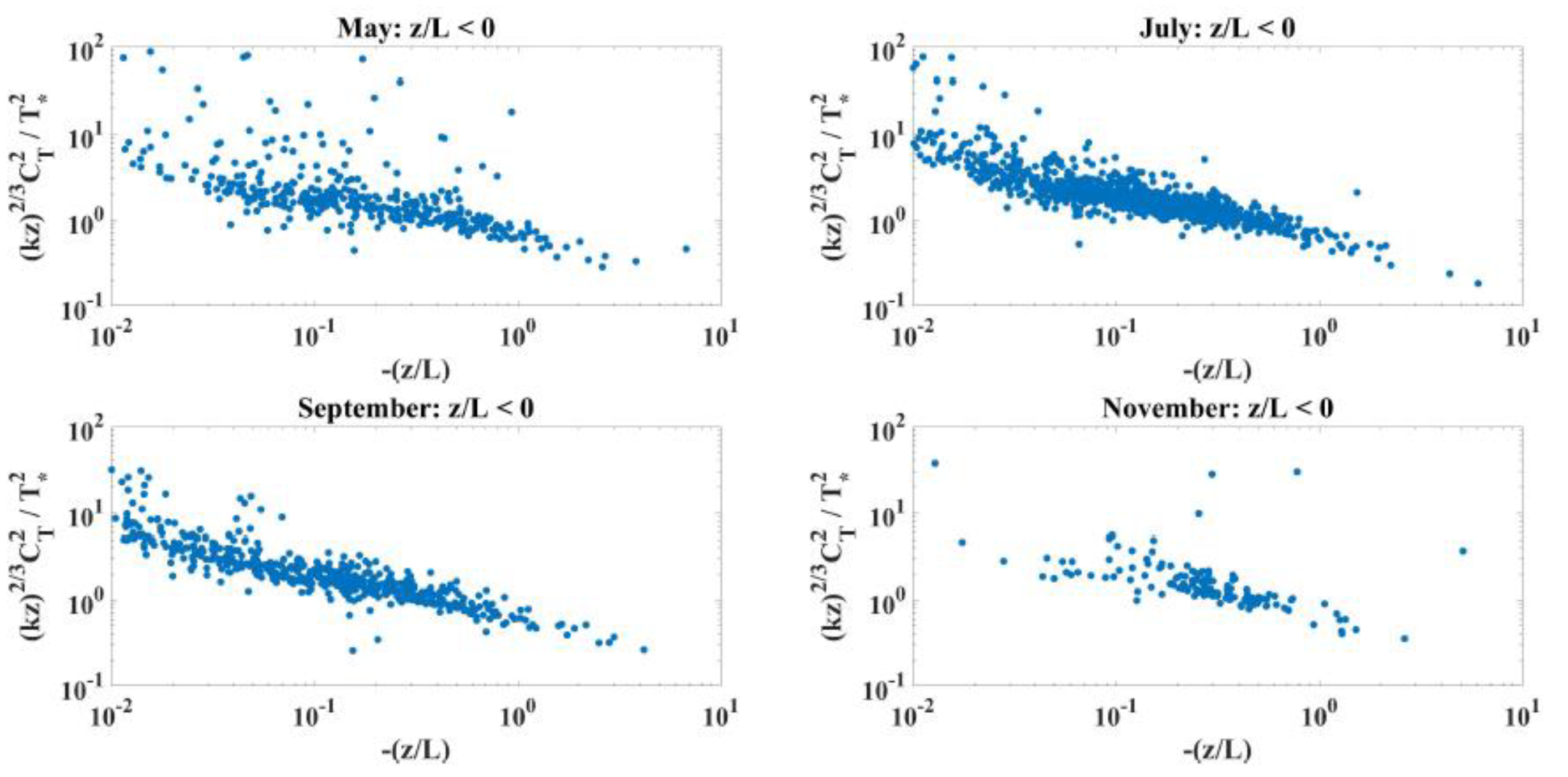
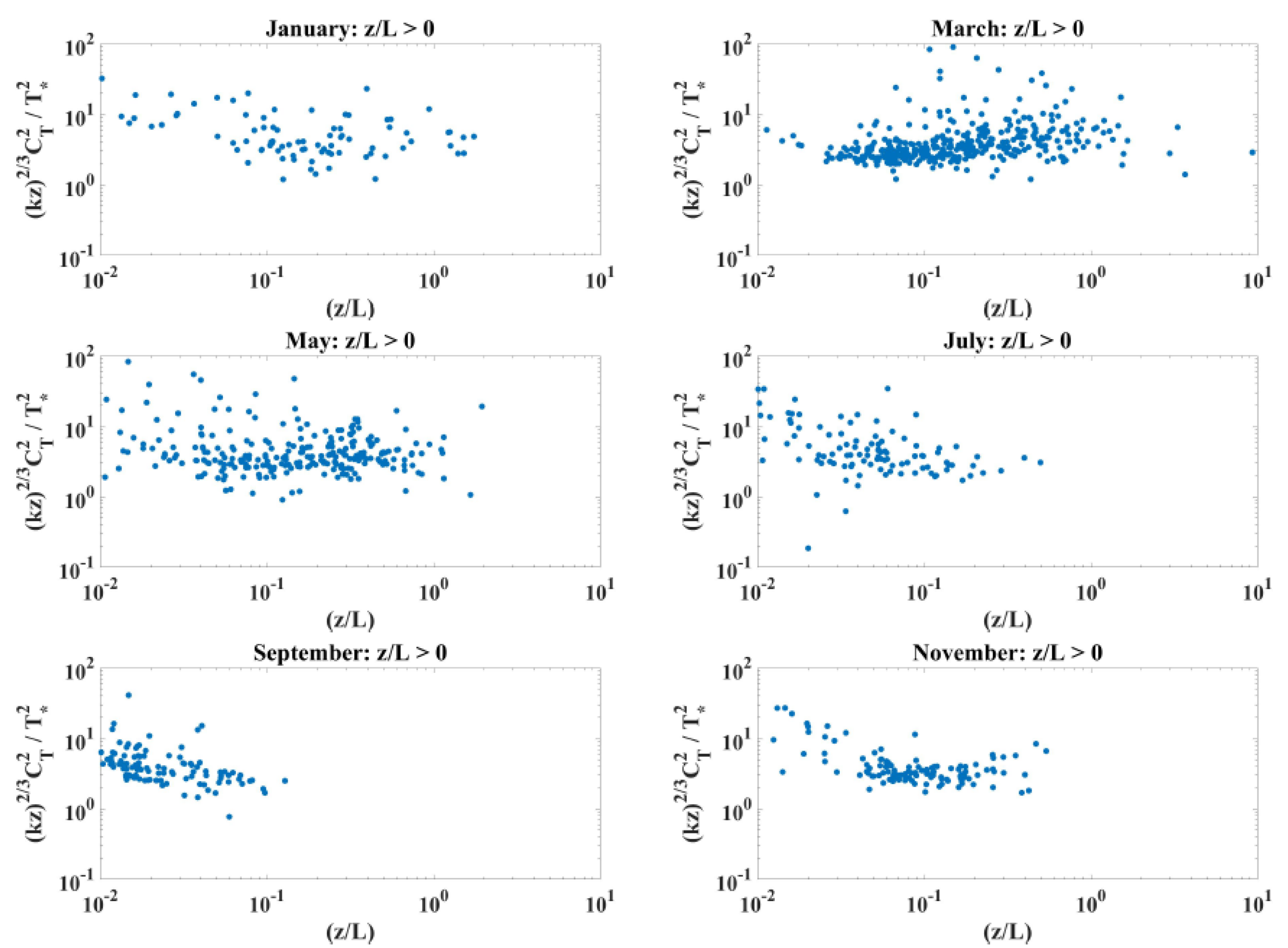
Figure 10 and Figure 11 show the normalized temperature structure coefficient by month for negative and positive conditions, respectively. Interestingly, these show that predictions under negative stability are better during the summer and fall months, even for the same z/L. This likely coincides with a strong air water temperature difference driving the vertical flux, even if the friction velocity is also large. These well-mixed conditions are likely to better match the assumptions required for Monin–Obukhov scaling. For positive z/L, there is very little data over the summer months making conclusions less robust. On the whole, we see a relatively constant temperature structure scaling once the near-neutral data are excluded. The variance in the data is also much larger for +z/L than for −z/L, leading to a general conclusion that other predictive tools are needed for this situation.

5. Conclusions

Optical turbulence characterization in a near-maritime environment is a complex and dynamic field of research, requiring an extensive understanding of the atmospheric surface layer. Over the course of 12 months, we collected velocity and sonic temperature measurements from a sensor suite constituting two CSAT3B sonic anemometers and one Infrared Gas Analyzer (IRGASON), deployed on a mast over the Chesapeake Bay in Annapolis, Maryland. This environment provided unique daily and seasonal variations compared to previous literature, which has reported predominantly terrestrial or fully maritime environments. We found that unstable conditions persisted throughout the summer and early fall months—when the surface waters are warmest—resulting in an unusual pattern of atmospheric stability. The temperature structure parameter showed less seasonal variation, from a monthly low of log($C_T^2$) = −2.62 to a high of −2.05 with a yearly average of −2.21. We also saw that the non-dimensional temperature structure parameter, from which optical propagation predictions can be made, scaled as expected during periods of atmospheric instability. We find that Monin–Obukhov similarity theory describes the structure of turbulence well under conditions of instability, which are common in this location. Among equal values of the stability parameter, this scaling was improved under conditions of high buoyant flux and high shear, which tended to match warm-water conditions in the late summer.