Article

A Machine Learning Approach for Air-Quality Forecast by Integrating GNSS Radio Occultation Observation and Weather Modeling

1
National Space Science Center, Chinese Academy of Sciences (NSSC/CAS), Beijing 100190, China
2
Beijing Key Laboratory of Space Environment Exploration, Beijing 100190, China
3
School of Astronomy and Space Science, University of Chinese Academy of Sciences, Beijing 100049, China
4
Joint Laboratory on Occultations for Atmosphere and Climate (JLOAC), National Space Science Center, CAS (NSSC/CAS) and University of Graz, Beijing 100190, China
5
Key Laboratory of Science and Technology on Space Environment Situational Awareness, Chinese Academy of Sciences, Beijing 100190, China
6
School of Civil and Resource Engineering, University of Science and Technology Beijing, Beijing 100083, China
7
National and Local Joint Engineering Laboratory for Big Data Analysis and Computer Technology, Beijing 100190, China
8
School of Petroleum Engineering, China University of Petroleum (East China), Qingdao 266580, China
9
Azureland Energy Technologies, Qingdao 266000, China
*
Authors to whom correspondence should be addressed.
Atmosphere 2023, 14(1), 58; https://doi.org/10.3390/atmos14010058
Submission received: 14 November 2022 / Revised: 15 December 2022 / Accepted: 17 December 2022 / Published: 28 December 2022
(This article belongs to the Section Atmospheric Techniques, Instruments, and Modeling)

Abstract

:
Air-quality monitoring and forecasting are crucial for atmosphere pollution control and management. We propose an innovative data-driven framework for air quality index (AQI) prediction by integrating GNSS radio occultation (GNSS-RO) observation and weather modeling. Empowered by the state-of-the-art machine learning approach, our method can effectively predict regional AQI with a comparable accuracy much more quickly than the traditional numerical modeling and simulation approach. In a real case study using a representative region of China, our data-driven approach achieves a 2000 times speedup; meanwhile, the prediction error measured by rRMSE is only 2.4%. We investigate further the effects of different models, hyperparameters, and meteorological factors on the performance of our AQI prediction framework, and reveal that wind field and atmospheric boundary-layer height are important influencing factors of AQI. This paper showcases a direct application of GNSS-RO observation in assisting in forecasting regional AQI. From a machine learning point of view, it provides a new way to leverage the unique merits of GNSS atmospheric remote sensing technology with the help of the more traditional weather forecasting modeling approach.

1. Introduction

1.1. Background and Motivation

Urban air pollution has been having a severe impact on public health and social activities [1,2]. In the endeavor of controlling and managing urban air pollution problems, the monitoring and evaluation of ambient air quality plays a vital role for governments and policymakers to design and formulate more effective air-pollution control measures and acts [3]. As a straightforward way of understanding and converting different air-pollution concentrations to a single number, AQI has been adopted widely by several countries and agencies for public information and data interpretation [4]. Thus, in this paper, we focus on the evaluation and, more importantly, the forecasting of AQI in a complex atmospheric system.
Physical models, such as weather research and forecasting (WRF) models, are commonly used to predict AQIs [5,6]. In essence, as a physics-based meteorological science research and simulation forecasting approach, WRF is used to obtain the distribution of the atmospheric wind field by counting observations of temperature, humidity, and pressure [7,8]. These observations can be used as boundary and initial conditions for forecasting meteorological parameters by such physical forward and assimilation models. However, although versatile and grounded by physical laws, the WRF approach is quite strict on the initial conditions, and the parameterization schemes with prediction accuracy heavily depend on the quality and abundance of model parameters. Moreover, as a grid-based computational approach, WRF is inherently computationally expensive and can easily become intractable when the domain of interest is beyond certain sizable areal coverage. Those drawbacks limit the capability of WRF in providing timely prediction, especially for a situation in which real-time forecasting is important [9,10].
On the other hand, data-driven approaches have made great progress in the recent decade [11,12]. Machine learning is widely used in functional integration applications due to its strong fitting ability. Compared with traditional physical forecasting models, machine learning models can greatly improve the speed of prediction by eliminating the need to construct a set of control equations to describe atmospheric motion patterns. Empowered by machine learning methods, data assimilation and model- prediction frameworks have exhibited the satisfactory performance in real-world applications [13].
In general, higher wind speed is more favorable for the dilution and diffusion of pollution in the air, whereas prolonged breezes or static wind tends to inhibit the diffusion of pollution and magnify the pollutants in the near-surface layer. At the bottom portion of the troposphere, the atmospheric boundary layer acts like a container to restrain the pollution concentration in the near-surface layer. The turbulence in the atmospheric boundary layer can accelerate the diffusion of air pollutants, and when the turbulence is limited, the pollutant concentration in the near-surface layer tends to increase.
Large-scale and fine-grained data collection of those abovementioned meteorological conditions has been a great challenge. The recent development of GNSS-RO remote sensing technology provides a promising way of obtaining several atmospheric parameters with a considerably high areal and vertical resolution with global coverage and high accuracy [14,15]. In addition, it has the advantages of self-correction, all-weather, real-time, long-term stability, and low cost. GNSS-RO can provide the derived atmospheric refractive index, which in turn correlates to atmospheric parameters, such as temperature, humidity, and air pressure [16,17,18]. Because GNSS-RO satellite orbits outside the atmosphere, there is no measurement error caused by temperature and other factors nor affected results by the deviation of space-based baselines [19]. Therefore, we take advantage of GNSS-RO’s unique strength in meteorological observations and utilize it to drive a newly designed machine learning framework for regional AQI prediction from a modern data-driven perspective.

1.2. Related Work

Realistic observations are crucial when conducting data-driven assimilation and prediction, whether they provide key pillars in the parameter space or important boundary, and initial conditions. Most previous studies predicting AQI have combined air-pollution observations with the forecasts of near-future meteorological conditions [20,21]. Among those meteorological conditions, temperature, humidity, pressure, wind speed, and boundary-layer height are critical because they affect the effectiveness of AQI prediction [22,23]. Dominick et al. argues that the concentration of air pollutants varies depending on meteorological factors, pollutant source intensity, the proximity of receptors, and local topography [24]. Revlett shows that ambient ozone concentrations are strongly correlated with atmospheric state, insolation, temperature, wind speed, and mixed layer depth [25].
Data-driven approaches using machine learning methods have shown good performance in dynamic systems in a variety of domains [26,27,28,29]. In addition, there are several recent studies applying machine learning methods for AQI prediction. Samal et al. proposed a new model-based bidirectional long short-term memory (BiLSTM) that provides nearly 16% better prediction performance enhancement than the common IDW method [30]. Sivakumar et al. used a multivariate linear regression machine learning model for AQI prediction in mining-based industrial areas for different sets of pollutant parameters [31]. Wang et al. indicate the superiority of LSTM in AQI prediction by comparing the performance of support vector regression (SVR), multilayer perceptron (MLP), backpropagation (BP), neural network, recurrent neural network (Simple RNN), and CT-LSTM methods for AQI prediction [32].
In the aspect of the utilization of GNSS-RO data in related atmospheric studies, in numerical weather prediction and tropical cyclone forecast, Bai et al. reviewed the application of GNSS-RO observations in numerical weather prediction (NWP) and tropical cyclone (TC) forecasting, illustrating that GNSS-RO measurements have made significant contributions to NWP and TC forecasting [33]. Chen et al. utilized the GSI hybrid assimilation system to assimilate RO data and the multiresolution global model (MPAS) to investigate the RO data impact on prediction of Typhoon Nepartak that passed over southern Taiwan in 2016 [34]. Ruston et al. summarized the impact of the FORMOSAT-7/COSMIC-2 GNSS-RO mission measurements in two independent NWP systems, which are now assimilating these measurements operationally [35].

1.3. Our Contribution

Although there have been numerous attempts to forecast AQI by using different approaches and their combinations, including numerical simulation and machine learning methods, to the best of our knowledge, we first use GNSS-RO observations to infer the forecasting of AQI in a carefully designed machine learning framework guided by WRF models. In essence, we propose a new approach to predict AQI efficiently and accurately. In comparison with physical model-based methods such as WRF, by using machine learning we eliminate the need to establish and solve complex and large governing equation systems, providing superior computational efficiency when making predictions.
This paper is structured as follows. In Section 2, we provide the methodology and describe in detail the workflow and procedures of our new data-driven framework for AQI prediction. In Section 3, we describe the Beijing–Tianjin–Hebei region from 50° N to 30° N and within 100° E to 130° E, as a representative region of study. In Section 4, we discuss the results of the newly proposed method by using real data for the study region as a critical performance assessment of the new method. We discuss the impacts and limitations of this work and outlook for future improvement in Section 5 with conclusions summarized in Section 6.

2. Methodology

2.1. Overall Workflow

The overall workflow is shown in Figure 1. In the data acquisition phase, we obtain data from ERA-interim as the initial field for the WRF model, which simulates temperature, humidity, pressure, wind field, and atmospheric boundary-layer height information. These data, combined with data from AQI monitoring stations, can be used for the training of wind field prediction models and AQI prediction models. In the model training phase, based on the data obtained in the previous phase, three neural network models—LSTM, convolutional neural network (CNN), and (deep neural network) DNN—are used to train the wind field prediction model, and the AQI prediction model, respectively. For the wind field prediction model, the inputs of the model are temperature, humidity, and pressure, and the output of the model is the predicted value of the wind field. For the AQI prediction model, the inputs to the model are historical data information of temperature, humidity, pressure, wind field, atmospheric boundary layer height, and AQI, and the output of the model is the predicted value of AQI for the next time. Because we are using a data-driven approach, we obtain GNSS-RO data from the European Centre for Medium-Range Weather Forecasts (ECMWF) in the model validation phase. The GNSS-RO data inversion allows us to obtain temperature, humidity, pressure, and atmospheric boundary-layer height information. By using the temperature, humidity, and pressure among them, the wind field information can be predicted by the wind field prediction model. Then, combined with the atmospheric boundary-layer height information, the AQI data at the next moment can be predicted by the AQI prediction model. Finally, we analyze the performance of the model driven by GNSS-RO data, the effect of different variables and hyperparameters on AQI prediction, and compare the effectiveness of different machine learning models and the required prediction time.

2.2. AQI

The AQI is a dimensionless index that quantitatively describes air-quality conditions. Its values can be used to communicate to the public the current level of air pollution. The AQI can be measured directly by AQI monitoring stations. The stations obtain measured concentrations of each pollutant such as fine particulate matter (PM2.5), respirable particulate matter (PM10), sulfur dioxide (SO2), nitrogen dioxide (NO2), ozone (O3), and carbon monoxide (CO). Based on the concentration values, the air-quality subindex (IAQI) can be calculated, and then the AQI can be calculated from Equation (1),
A Q I = m a x ( I A Q I 1 , I A Q I 2 , . . . , I A Q I n ) ,
where, I A Q I P represents the air-quality subindex of pollutant item P in the corresponding area and n represents the pollutant item.
Different AQI values correspond to different classifications and have different levels of health effects. Laymen do not need to remember the specific AQI values and levels, but only need to pay attention to the six evaluation categories and characterization colors, such as excellent (green), good (yellow), light pollution (orange), moderate pollution (red), heavy pollution (purple), and severe pollution (maroon), etc. The larger the AQI value, the higher the level and category, and the darker the characterization color, the more serious the air pollution condition, and the greater the health risk to humans.

2.3. Data Collection

2.3.1. Data from Monitoring Station

The ERA-interim dataset from ECMWF is a reanalysis of the rich global atmospheric data available since 1979. In this paper, ERA-interim data are used as the initial condition, including temperature, humidity, pressure, wind field, boundary-layer height, etc. for each time instant [36,37].
The AQI data used in this paper are from the China National Environmental Monitoring Center, and some of the AQI data are missing due to local conditions. In this study, the AQI data are automatically interpolated by appropriate methods using data from other nearby observation stations to obtain the local AQI. For the area from 50° N to 30° N and 100° E to 130° E, a grid with a resolution of 0.25 degrees was chosen. We selected 33 monitoring stations in the Beijing–Tianjin–Hebei region. For each monitoring station point, we choose the temperature, humidity, pressure, wind field, atmospheric boundary-layer height, and AQI information for one month, one data every three hours. Therefore, the scale of input data is 33 × 120 × 7. The output data is the AQI at the next moment. Therefore, the size of the output data is 33 × 120 × 1.

2.3.2. Data from WRF

The numerical model WRF can be used to numerically simulate and forecast the wind field in the Beijing–Tianjin–Hebei region. In our previous study, we used a double-nested grid scheme to simulate and calculate the wind field conditions in the whole Beijing–Tianjin–Hebei region [38]. Here, we use the derived meteorological parameters from WRF to train the machine learning models. The input of the WRF model is the ERA-interim dataset. We are not at liberty to disclose the parameters of the WRF model, but there are various classical WRF models for wind field and atmospheric boundary-layer height predictions available for the reader to reproduce.

2.3.3. Data from GNSS-RO

The Catalogue of Somatic Mutations in Cancer (COSMIC) occultation data from June 2018 to July 2019 were chosen for this study, and each occultation event was classified by time period. At each time period, the temperature, humidity, and pressure of each profile are interpolated according to the same grid division as ERA-interim and collated into the GNSS-RO dataset. Before interpolation, the data first need to be preprocessed. Because the GNSS-RO dataset is from a different source than the WRF dataset, a normalization method needs to be used to achieve unity in the probability distribution of the two datasets [39,40].
One occultation event can only provide the occultation data profile of the satellite location at a certain time, so the weather data of the predicted area needs to be obtained by interpolation. Each occultation event is classified by time period, and the time period in which at least seven occultations occurred in the Beijing–Tianjin–Hebei region within two hours is selected, and the temperature, humidity, and pressure are interpolated according to the same grid division as the ERA-interim to extract the temperature, humidity, and pressure at the corresponding latitude and longitude.

2.4. Neural Network Models

Wind and AQI field prediction are essentially spatial–temporal problems. LSTM is one of the most widely used algorithms to solve time sequence-related modeling, and CNN is suitable for image-based or spatially resolved problems [41,42,43]. Meanwhile, DNN generally outperforms the traditional shallow architecture of machine learning models by additional processing layers (e.g., adaptive layers). Therefore, we choose three neural network models—LSTM, CNN, and DNN—to train the AQI prediction model. In this paper, we use the PyTorch framework to build neural network models.

2.4.1. LSTM

LSTM is a special recurrent neural network designed to solve the problem of gradient disappearance and gradient explosion during training of long sequences, which requires remembering what needs to be remembered for a long time and forgetting the unimportant information. The LSTM generally outperforms other neural network models for tasks that require “long-term memory”. There are three main phases within the LSTM: the forgetting phase, the selection memory phase, and the output phase [44,45]. The LSTM network trains the long-term and short-term memory parameters of each module to achieve a balance between long-term and short-term memory. The neural network is continuously updated with iterations, and for each time instant, a matrix of weights is trained to represent the degree of memory and forgetting [44].
In this paper, the LSTM model uses one LSTM layer and one fully connected layer, and the init condition of the LSTM layer contains two random vectors. Algorithm 1 reveals the architecture of the model.    
Algorithm 1: LSTM architecture
1 initialization;
2 x = LSTM(input_size, hidden_size = 32, num_layers = 4)(input);
3 output = full_connect(hidden_size = 32, output_size)(x);
4 return output;

2.4.2. CNN

A CNN is a feedforward neural network and is one of the most widely used deep learning algorithms. A CNN consists of the following five kinds of layers: input layer, convolutional layer, pooling layer, fully connected layer, and output layer. Compared with other neural networks, the advantage of the CNN in prediction performance is that the features of the input can be extracted by convolution and pooling. The convolutional layer extracts features through the dot product of the convolutional kernel and the training set data. The pooling layer processes the data from the convolutional layer to reduce the feature dimensionality. Due to the convolutional and pooling layers, CNNs have good performance in extracting features from the input data [46].
In this paper, the CNN model uses two convolutional layers and one fully connected layer, and the convolutional kernel size is 1 × 1, and the output size of the fully connected layer is 5 because the batch size is 5. Algorithm 2 reveals the architecture of the model.    
Algorithm 2: CNN architecture
1 initialization;
2 x = conv(input_size, hidden_size, kernel_size = 1)(input);
3 x = conv(hidden_size, 1, kernel_size = 1)(x);
4 x = full_connect(input_size, 32)(x);
5 x = full_connect(32, 10)(x);
6 output = linear(10, output_size)(x);
7 return output;

2.4.3. DNN

The DNN uses a backpropagation algorithm consisting of multiple layers of perceptrons. It is a kind of multilayer feedforward neural network. the DNN algorithm consists of two stages: signal forward propagation and error backward propagation. Forward propagation is the process of prediction results and error output from input to output; backward propagation is the process of adjusting weights and thresholds from output to input. The training results are recorded in the form of weights and thresholds for each neuron. By repeating the two stages of forward and backward propagation, the neural network is continuously trained so that the predicted value is closest to the true value [46].
In this paper, the DNN model uses two fully connected layers. Algorithm 3 reveals the architecture of the model.   
Algorithm 3: DNN architecture
1 initialization
2 x = full_connect(input_size, hidden_size_1)(input)
3 x = full_connect(hidden_size_1, hidden_size_2)(x)
4 output = full_connect(hidden_size_2, output_size)(x)
5 return output;

2.5. Process of Train and Validation

When building a network model, the data needs to be preprocessed first. The data preprocessing can reduce the poor generalization ability of the neural network model due to data characteristics and to reduce the error. The data ranges of the input features are not consistent, and the excessive data bias is not conducive to the processing of neural networks. Therefore, this study uses normalization to eliminate the problem of poor training effect and training speed of neural networks due to different ranges of sample data. In addition, it is also able to eliminate the effect of magnitude. By normalizing both input and output features and reducing the range of variables to [0, 1], the equation of the new variable A after normalization is obtained in Equation (2),
A = A m i n ( A ) m a x ( A ) m i n ( A ) ,
where m i n ( A ) denotes the minimum value of the variable A, m a x ( A ) denotes the maximum value of the variable A.
When building the network model, the activation function needs to be considered. The rectified linear unit (ReLU) function is chosen for the activation functions of all three neural networks in this project. The ReLU function can control the activation state of neurons, and the gradient descent and backpropagation efficiency of the ReLU function is more efficient than other activation functions in gradient descent and backpropagation, which can effectively avoid the gradient explosion and gradient disappearance problems. The expression of the ReLU function is shown in Equation (3):
R e L U ( x ) = m a x ( 0 , x ) .
The loss function also needs to be considered when building the network model. For the AQI prediction, the relative root mean squared error (rRMSE) is used as the test. r R M S E is calculated by the formula in Equation (4),
r R M S E = R M S E p ¯ ,
where rRMSE is the relative root mean squared error, RMSE is the root mean squared error, and p ¯ is the measured mean value.

3. Study Area

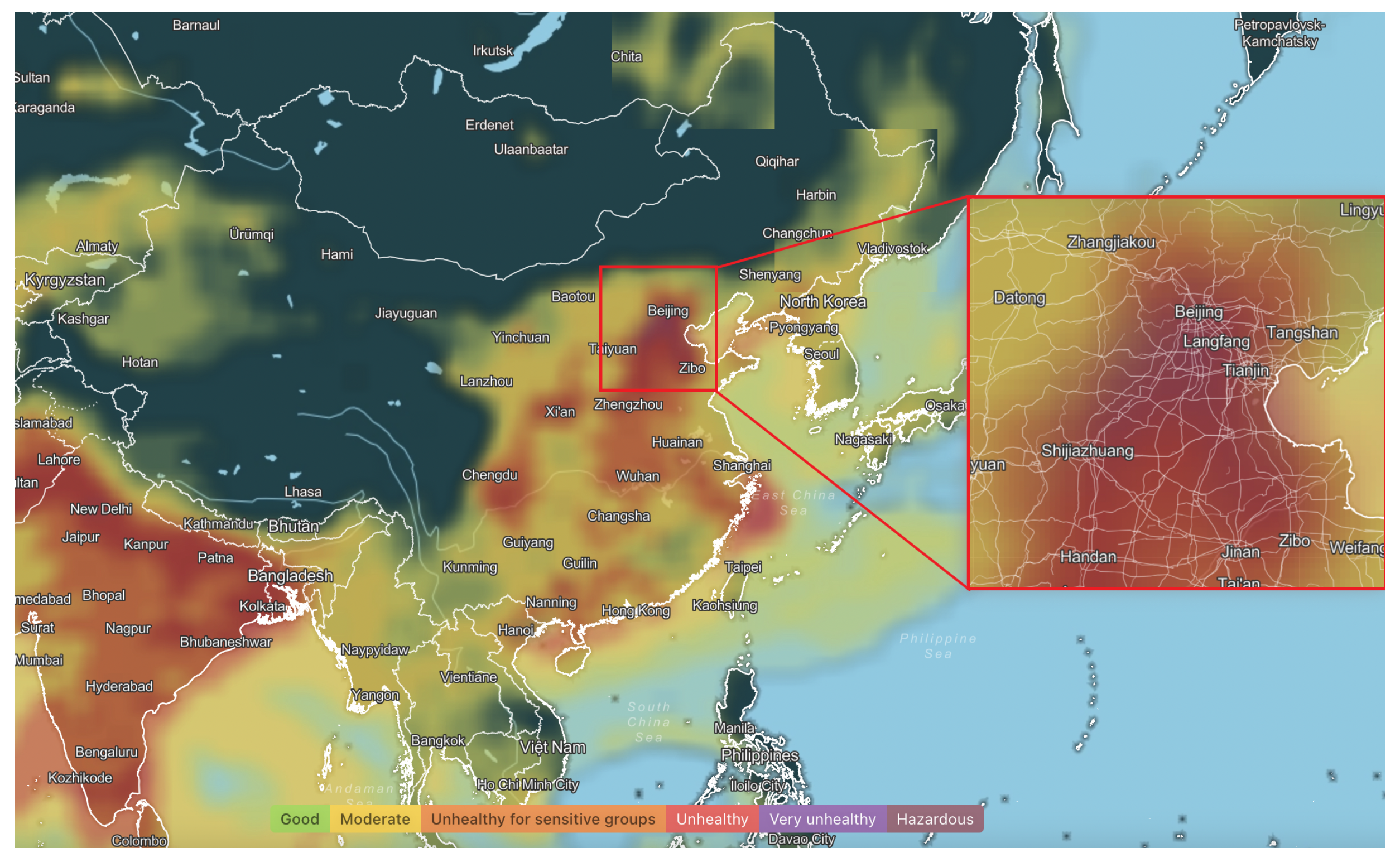
The Beijing–Tianjin–Hebei area is one of the most highly populated and industrialized regions in China with high traffic flow and heavy air pollution. Air pollution has been a significant problem for this region. Measures act and practices have been taken into place during the past decade to mitigate the air pollution issue [47]. Among them, AQI monitoring and forecasting are of great importance. Therefore, in this paper, we choose Beijing–Tianjin–Hebei as a representative case study. The horizontal coverage of the study area of this project is from 50° N to 30° N and 100° E to 130° E, as shown in Figure 2.

4. Results and Discussions

4.1. Effect of Different Neural Network Models on AQI Prediction

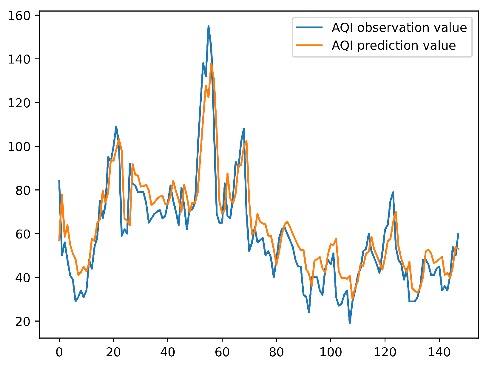
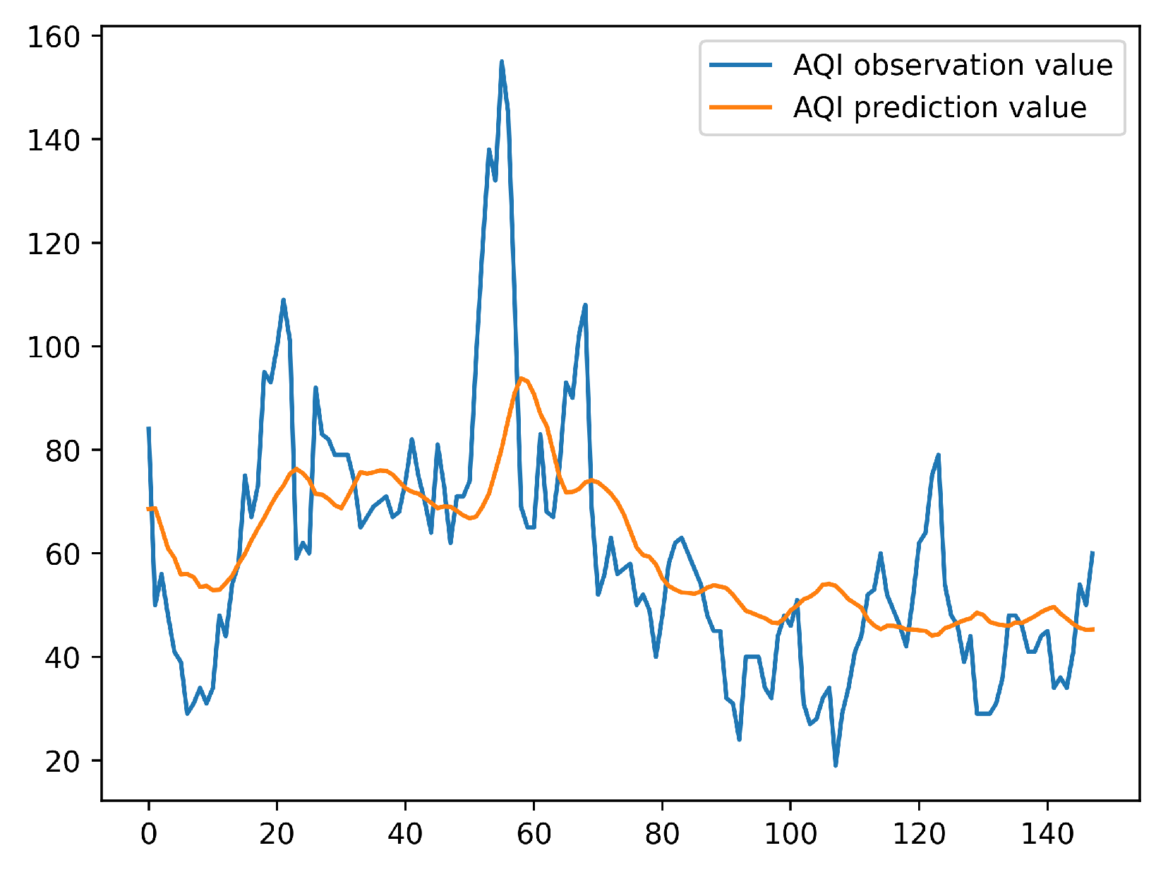
We implement three different neural network models, LSTM, CNN, and DNN for AQI prediction. The results of each neural network model for the next 3 h of AQI forecast are shown in Figure 3, Figure 4 and Figure 5.
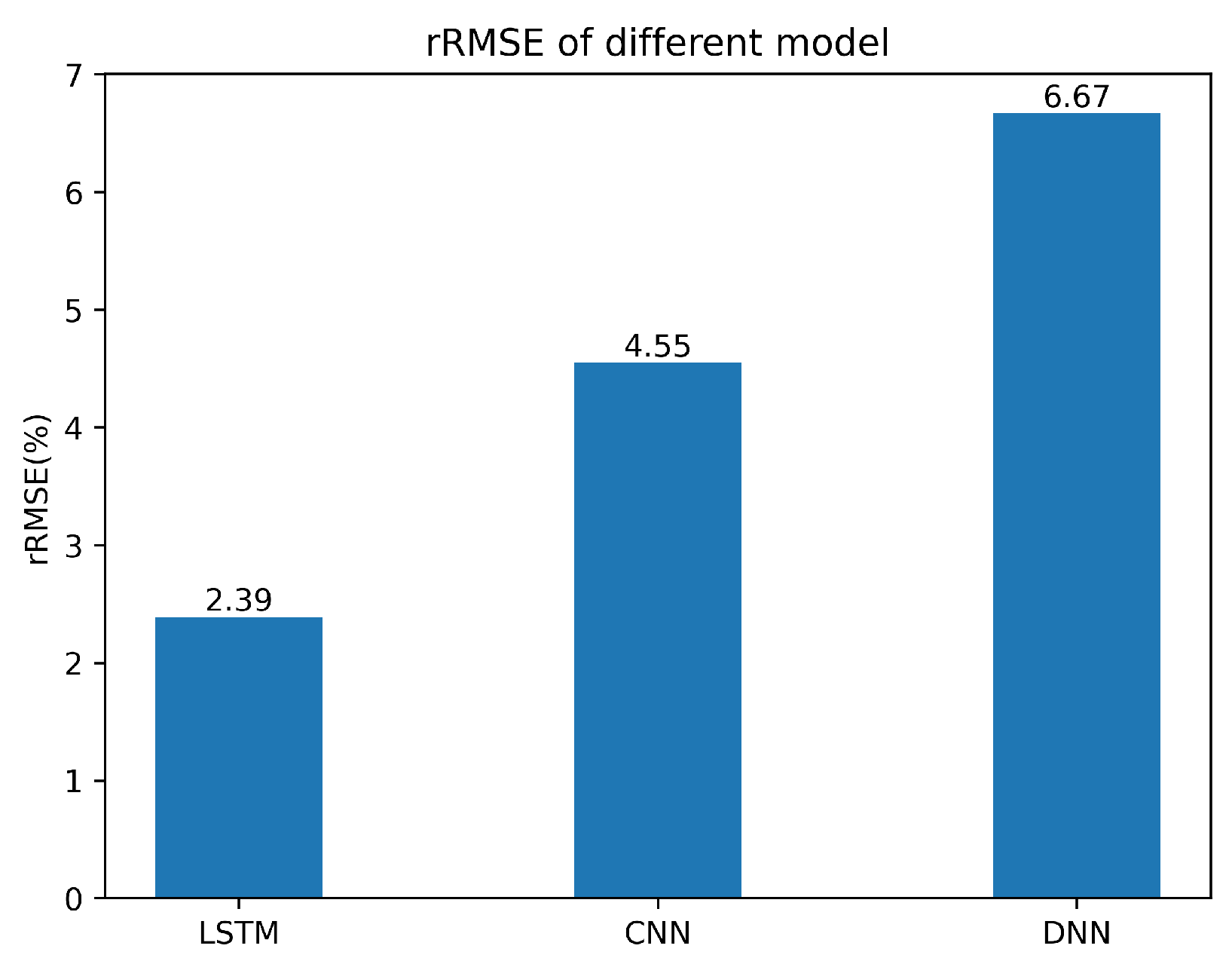
Figure 6 exhibits the errors of the AQI forecast by those three different neural networks. As can be seen in Figure 6, the rRMSE of LSTM is 2.39%, the rRMSE of CNN is 4.55%, and the rRMSE of DNN is 6.67%, respectively, which indicates that LSTM outperforms the other two models in prediction accuracy.
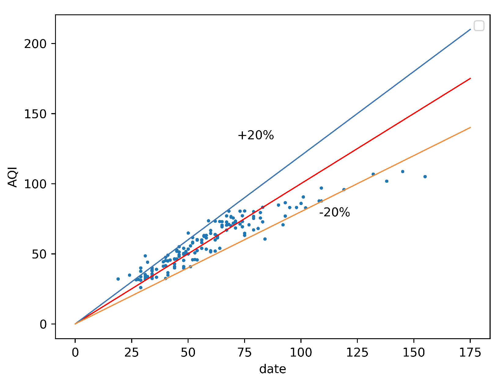
For a selected location of the center of the simulation domain at 115 E and 40 N, Figure 7 shows the comparison between the predicted and observed AQI values using the LSTM model. The axis indicates the predicted value of the neural network, and the vertical axis indicates the observed value. The closer the points in the plot are to the line y = x , the closer the predicted value and the monitored value are to each other. Thus, the prediction performance of the neural network can be readily obtained from the distribution of the scattered points. From Figure 7, it is found that LSTM has good performance because most of the points are around the line y = x scattering within an error range of ± 20 % .

4.2. Impact of the Ratio of the Training Set and Test Set on AQI Prediction

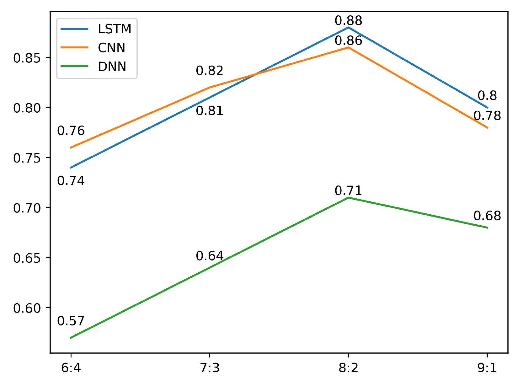
In the field of machine learning, it is important to divide the training set and test set reasonably. We filtered the dataset division with the smallest rRMSE by adjusting the ratio of the training set and test set in the dataset with other parameters unchanged. The effect of different division ratios on the training effect is shown in Figure 8, from which it can be seen that the best division ratio is 8:2 between the training and test sets. When the ratio of the training set is too low, the training effect is not good because there are not enough samples for support; when the ratio is more than 8:2, the ratio of the test set is too low, and the reflection of the training effect is not enough. Through comparison, 8:2 was determined to be the best dataset division for this study model.

4.3. Impact of Meteorological Parameters on AQI Prediction

Among the meteorological parameters, not all of them have significant impacts on AQI prediction. On the contrary, too many features with low correlation can lead to compromised neural network training effectiveness and speed. Therefore, the effects of different meteorological parameters on AQI prediction effectiveness need to be analyzed. Permutation importance provides a model-independent method for calculating feature importance, which randomly shuffles all values of a feature on the dataset and illustrates the importance of the feature by the difference between old and new prediction results.
We respectively shuffle the five features of wind speed, temperature, humidity, pressure, and boundary-layer height. Figure 9 shows the obtained results. The bar height corresponds to the importance of each feature. It can be seen that the boundary layer height is the most important feature, followed by temperature, wind speed, humidity, and pressure in that order. Among the five features, the atmospheric boundary layer height is the most important, wind speed is more sensitive than humidity and pressure, and wind speed and atmospheric boundary layer height are the top two influencing factors of AQI.
To further illustrate the effects of wind fields and atmospheric boundary-layer height on AQI predictions, an ablation test was conducted. The ablation test is similar to the control variables method by eliminating the effect of a particular feature observation on the results. The results of the ablation experiment are shown in Table 1. By analyzing the results of the ablation experiment, the importance of a particular feature in the model can be determined. Here, we tested the experiments combining wind field, combining atmospheric boundary-layer height, and combining both wind field and atmospheric boundary-layer height, using temperature, humidity, and pressure as features as the baseline. The results of the ablation tests show that both wind field and atmospheric boundary-layer height have important effects on the results. In summary, we believe that wind field and atmospheric boundary-layer height are important influencing factors of AQI.

4.4. Effect of Hyperparameters on AQI Prediction

In deep learning, hyperparameters have an important impact on the prediction effectiveness of the model. In this study, the main hyperparameters involved are the learning rate and the epoch of iterations. The learning rate is the magnitude of updating the network weights in the optimization algorithm, and it is critical to the algorithm’s performance. The epoch of iterations is the number of training times of the entire training set when it is fed into the neural network, and the number of iterations can be considered appropriate when the difference between the validation error rate and the training error rate is small.
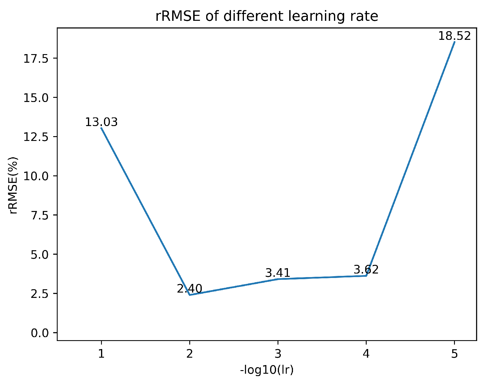
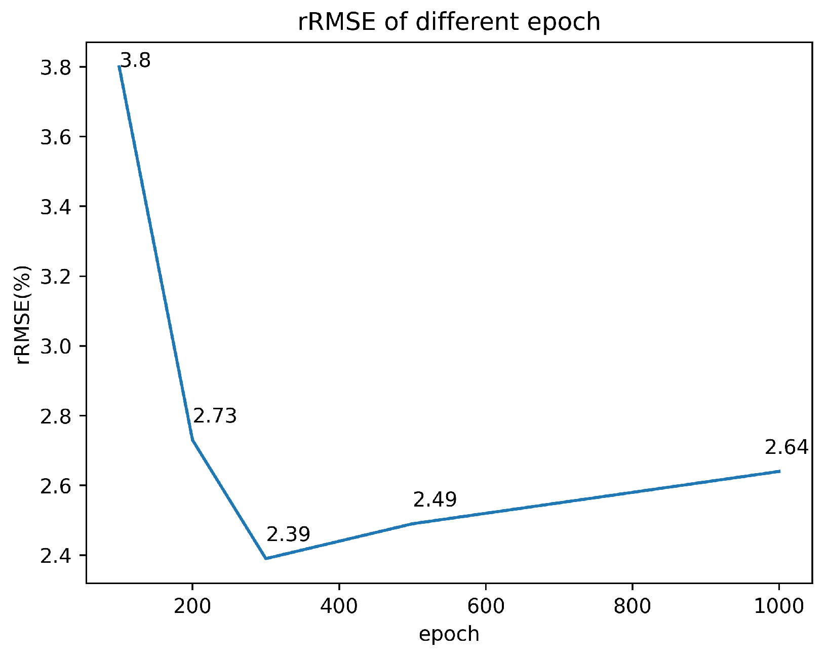
Figure 10 shows the rRMSEs of the models trained with different learning rates. It is apparent that as the learning rate decreases, the model first performs better and then becomes worse on the test set. This is because a large learning rate tends to cause the parameters to oscillate back and forth on both sides of the optimal solution, and a small learning rate slows down model convergence. Figure 11 shows the rRMSE of the model at the different number of iterations of training on the test set, and the model performs best when the selected number of iterations is 300. The model does not work well due to the poor fitting ability when the number of iterations is less than 300. On the other hand, the overfitting phenomenon tends to occur, when the number of iterations keeps increasing.

4.5. Prediction Time of Different Prediction Models

This experiment was conducted by using a desktop computer with 32 GiB RAM, 12-core CPU, and RTX 3060 graphics card for training. To evaluate the computational efficiency, we conduct the comparison of prediction time of different data-driven methods as well as the WRF approach in Table 2. Among the four models, LSTM, CNN, DNN, and WRF, the WRF model does not require training time, but uses the longest prediction time of about 15 min and 32 s; the DNN model has the shortest training time, with training time and prediction time of 31 s and 0.48 s, respectively. The LSTM model has the longest training time and prediction time of 1 min and 42 s and 0.46 s, respectively. the CNN model has the training time and prediction time between the DNN model and the LSTM model with 1 min 2 s and 0.47 s, respectively. Because the deployment model is used for prediction, only the prediction time needs to be considered. Combined with the actual prediction results, we choose the LSTM model for application deployment. The prediction time of the LSTM method is improved by more than 2000 times compared with the WRF model, and the method provides a good prospect for fast forecasting of AQI.

5. Limitations and Expected Impacts

We propose an AQI prediction method driven by GNSS-RO data, which is location-independent and can achieve real-time AQI prediction in all weather as long as GNSS-RO data and historical AQI observations are available. For edge-end devices that can only receive GNSS-RO data, our method has good AQI prediction results. However, there are still many directions for improvement in the future. On the one hand, we use the classical neural network model for AQI prediction and do not investigate the neural network model architecture. On the other hand, the sources of training and validation data are different (WRF & GNSS-RO), and we only used data normalization to preprocess the dataset.
Future work can build on our work and try to validate more complex LSTM models. In the future, there are plans to launch more GNSS-RO satellites and we will obtain enough GNSS-RO data for training. After obtaining enough data, we can consider using the GNSS-RO dataset as the training set for the machine learning model to achieve consistency in data distribution. It is also a good idea to use the incremental method of small sample data for model training.

6. Conclusions

In summary, we propose a new data-driven method for rapid AQI forecasting that integrates GNSS-RO meteorological observations and weather modeling under a modern machine-learning framework. By using the Beijing–Tianjin–Hebei region as a real-world case study, we implement the new approach for AQI forecasting performance evaluation. Our approach achieves 2000 times speedup in comparison with the traditional physics-based models. As the core of the machine learning approach, we compare the performance of three neural network models, namely, LSTM, CNN, and DNN for GNSS-RO data assimilation. The prediction results show that the LSTM model performs the best in terms of prediction accuracy with a calculated rRMSE of 2.4%. We also provide the analysis of different meteorological parameters and hyperparameters to understand their influence on AQI results and algorithmic performance. Thus, together with the advantages of GNSS-RO remote sensing in terms of correctness, coverage, and resolution, our new method is promising for rapid AQI forecasting and worthy of further studies to explore the prediction accuracy and efficiency by using more advanced machine learning models in more complex scenarios.

Author Contributions

Methodology, W.L., W.B.; writing—original draft preparation, S.K.; supervision, Y.S.; project administration, H.S., Y.W. All authors have read and agreed to the published version of the manuscript.

Funding

This research was supported by the National Natural Science Foundation of China, grant numbers 42104032 and 42074042; Key Program of Joint Fund of the National Natural Science Foundation of China and Shandong Province under Grant U22A20586; Youth Cross Team Scientific Research Project of the Chinese Academy of Sciences (JCTD-2021-10); FengYun Application Pioneering Project (FY-APP-2022.0108).

Conflicts of Interest

The authors declare no conflict of interest.

References

  1. Brunekreef, B.; Holgate, S.T. Air pollution and health. Lancet 2002, 360, 1233–1242. [Google Scholar] [CrossRef] [PubMed]
  2. Kampa, M.; Castanas, E. Human health effects of air pollution. Environ. Pollut. 2008, 151, 362–367. [Google Scholar] [CrossRef] [PubMed]
  3. Brunekreef, B. Health effects of air pollution observed in cohort studies in Europe. J. Expo. Sci. Environ. Epidemiol. 2007, 17, S61–S65. [Google Scholar] [CrossRef] [PubMed]
  4. Chen, W.; Wang, F.; Xiao, G.; Wu, K.; Zhang, S. Air Quality of Beijing and Impacts of the New Ambient Air Quality Standard. Atmosphere 2015, 6, 1243–1258. [Google Scholar] [CrossRef] [Green Version]
  5. Zhu, S.; Lian, X.; Liu, H.; Hu, J.; Wang, Y.; Che, J. Daily air quality index forecasting with hybrid models: A case in China. Environ. Pollut. 2017, 231, 1232–1244. [Google Scholar] [CrossRef] [PubMed]
  6. Jiang, C.; Wang, H.; Zhao, T.; Li, T.; Che, H. Modeling study of PM2.5 pollutant transport across cities in China’s Jing–Jin–Ji region during a severe haze episode in December 2013. Atmos. Chem. Phys. 2015, 15, 5803–5814. [Google Scholar] [CrossRef] [Green Version]
  7. Solbakken, K.; Birkelund, Y.; Samuelsen, E.M. Evaluation of surface wind using WRF in complex terrain: Atmospheric input data and grid spacing. Environ. Model. Softw. 2021, 145, 105182. [Google Scholar] [CrossRef]
  8. Liu, Y. Relationships of wind speed and precipitable water vapor with regional PM2.5 based on WRF-Chem model. Nat. Resour. Model. 2021, 34, e12306. [Google Scholar] [CrossRef]
  9. Zhang, Y.; Bocquet, M.; Mallet, V.; Seigneur, C.; Baklanov, A. Real-time air quality forecasting, part I: History, techniques, and current status. Atmos. Environ. 2012, 60, 632–655. [Google Scholar] [CrossRef]
  10. Hutchison, K.D.; Smith, S.; Faruqui, S.J. Correlating MODIS aerosol optical thickness data with ground-based PM2.5 observations across Texas for use in a real-time air quality prediction system. Atmos. Environ. 2005, 39, 7190–7203. [Google Scholar] [CrossRef]
  11. Solomatine, D.; See, L.; Abrahart, R. Data-Driven Modelling: Concepts, Approaches and Experiences. In Practical Hydroinformatics: Computational Intelligence and Technological Developments in Water Applications; Abrahart, R.J., See, L.M., Solomatine, D.P., Eds.; Water Science and Technology Library; Springer: Berlin/Heidelberg, Germany, 2008; pp. 17–30. [Google Scholar] [CrossRef]
  12. Provost, F.; Fawcett, T. Data Science and its Relationship to Big Data and Data-Driven Decision Making. Big Data 2013, 1, 51–59. [Google Scholar] [CrossRef] [PubMed]
  13. Buizza, C.; Quilodrán Casas, C.; Nadler, P.; Mack, J.; Marrone, S.; Titus, Z.; Le Cornec, C.; Heylen, E.; Dur, T.; Baca Ruiz, L.; et al. Data Learning: Integrating Data Assimilation and Machine Learning. J. Comput. Sci. 2022, 58, 101525. [Google Scholar] [CrossRef]
  14. Chan, K.M.; Wood, R. The seasonal cycle of planetary boundary layer depth determined using COSMIC radio occultation data. J. Geophys. Res. Atmos. 2013, 118, 12,422–12,434. [Google Scholar] [CrossRef]
  15. Guo, P.; Kuo, Y.H.; Sokolovskiy, S.V.; Lenschow, D.H. Estimating Atmospheric Boundary Layer Depth Using COSMIC Radio Occultation Data. J. Atmos. Sci. 2011, 68, 1703–1713. [Google Scholar] [CrossRef]
  16. Zakharov, V.I.; Kunitsyn, V.E. Possibilities of radio occultation sounding using the GPS/GLONASS system for regional monitoring of the atmosphere. Mosc. Univ. Phys. Bull. 2007, 62, 260–265. [Google Scholar] [CrossRef]
  17. Wickert, J.; Reigber, C.; Beyerle, G.; König, R.; Marquardt, C.; Schmidt, T.; Grunwaldt, L.; Galas, R.; Meehan, T.K.; Melbourne, W.G.; et al. Atmosphere sounding by GPS radio occultation: First results from CHAMP. Geophys. Res. Lett. 2001, 28, 3263–3266. [Google Scholar] [CrossRef] [Green Version]
  18. Steiner, A.K.; Kirchengast, G.; Ladreiter, H.P. Inversion, error analysis, and validation of GPS/MET occultation data. Ann. Geophys. 1998, 17, 122–138. [Google Scholar] [CrossRef] [Green Version]
  19. Bonafoni, S.; Biondi, R. The usefulness of the Global Navigation Satellite Systems (GNSS) in the analysis of precipitation events. Atmos. Res. 2016, 167, 15–23. [Google Scholar] [CrossRef]
  20. Díaz-Fernández, J.; Bolgiani, P.; Santos-Muñoz, D.; Sastre, M.; Valero, F.; Sebastián-Martín, L.I.; Fernández-González, S.; López, L.; Martín, M.L. On the characterization of mountain waves and the development of a warning method for aviation safety using WRF forecast. Atmos. Res. 2021, 258, 105620. [Google Scholar] [CrossRef]
  21. Cheng, W.L.; Chen, Y.S.; Zhang, J.; Lyons, T.J.; Pai, J.L.; Chang, S.H. Comparison of the Revised Air Quality Index with the PSI and AQI indices. Sci. Total Environ. 2007, 382, 191–198. [Google Scholar] [CrossRef]
  22. Cao, B.; Wang, X.; Ning, G.; Yuan, L.; Jiang, M.; Zhang, X.; Wang, S. Factors influencing the boundary layer height and their relationship with air quality in the Sichuan Basin, China. Sci. Total Environ. 2020, 727, 138584. [Google Scholar] [CrossRef] [PubMed]
  23. Njuki, S.M.; Mannaerts, C.M.; Su, Z. Influence of Planetary Boundary Layer (PBL) Parameterizations in the Weather Research and Forecasting (WRF) Model on the Retrieval of Surface Meteorological Variables over the Kenyan Highlands. Atmosphere 2022, 13, 169. [Google Scholar] [CrossRef]
  24. Dominick, D.; Latif, M.T.; Juahir, H.; Aris, A.; Zain, S. An assessment of influence of meteorological factors on PM10 and NO2 at selected stations in Malaysia. Sustain. Environ. Res. 2012, 22, 305–315. [Google Scholar]
  25. Revlett, G.H. Ozone Forecasting Using Empirical Modeling. J. Air Pollut. Control. Assoc. 1978, 28, 338–343. [Google Scholar] [CrossRef]
  26. Farchi, A.; Laloyaux, P.; Bonavita, M.; Bocquet, M. Using machine learning to correct model error in data assimilation and forecast applications. Q. J. R. Meteorol. Soc. 2021, 147, 3067–3084. [Google Scholar] [CrossRef]
  27. Du, S.; Wang, R.; Wei, C.; Wang, Y.; Zhou, Y.; Wang, J.; Song, H. The Connectivity Evaluation Among Wells in Reservoir Utilizing Machine Learning Methods. IEEE Access 2020, 8, 47209–47219. [Google Scholar] [CrossRef]
  28. Abarbanel, H.D.I.; Rozdeba, P.J.; Shirman, S. Machine Learning: Deepest Learning as Statistical Data Assimilation Problems. Neural Comput. 2018, 30, 2025–2055. [Google Scholar] [CrossRef]
  29. Jose, D.M.; Vincent, A.M.; Dwarakish, G.S. Improving multiple model ensemble predictions of daily precipitation and temperature through machine learning techniques. Sci. Rep. 2022, 12, 4678. [Google Scholar] [CrossRef] [PubMed]
  30. Samal, K.; Babu, K.; Das, S. Spatio-temporal Prediction of Air Quality using Distance Based Interpolation and Deep Learning Techniques. EAI Endorsed Trans. Smart Cities 2021, 5, e4. [Google Scholar] [CrossRef]
  31. Sigamani, S.; Venkatesan, R. Air quality index prediction with influence of meteorological parameters using machine learning model for IoT application. Arab. J. Geosci. 2022, 15, 340. [Google Scholar] [CrossRef]
  32. Wang, J.; Li, J.; Wang, X.; Wang, J.; Huang, M. Air quality prediction using CT-LSTM. Neural Comput. Appl. 2021, 33, 4779–4792. [Google Scholar] [CrossRef]
  33. Bai, W.; Deng, N.; Sun, Y.; Du, Q.; Xia, J.; Wang, X.; Meng, X.; Zhao, D.; Liu, C.; Tan, G.; et al. Applications of GNSS-RO to Numerical Weather Prediction and Tropical Cyclone Forecast. Atmosphere 2020, 11, 1204. [Google Scholar] [CrossRef]
  34. Chen, S.Y.; Shih, C.P.; Huang, C.Y.; Teng, W.H. An Impact Study of GNSS RO Data on the Prediction of Typhoon Nepartak (2016) Using a Multiresolution Global Model with 3D-Hybrid Data Assimilation. Weather. Forecast. 2021, 36, 957–977. [Google Scholar] [CrossRef]
  35. Ruston, B.; Healy, S. Forecast Impact of FORMOSAT-7/COSMIC-2 GNSS Radio Occultation Measurements. Atmos. Sci. Lett. 2021, 22, e1019. [Google Scholar] [CrossRef]
  36. Dee, D.P.; Uppala, S.M.; Simmons, A.J.; Berrisford, P.; Poli, P.; Kobayashi, S.; Andrae, U.; Balmaseda, M.A.; Balsamo, G.; Bauer, P.; et al. The ERA-Interim reanalysis: Configuration and performance of the data assimilation system. Q. J. R. Meteorol. Soc. 2011, 137, 553–597. [Google Scholar] [CrossRef]
  37. Berrisford, P.; Kållberg, P.; Kobayashi, S.; Dee, D.; Uppala, S.; Simmons, A.J.; Poli, P.; Sato, H. Atmospheric conservation properties in ERA-Interim. Q. J. R. Meteorol. Soc. 2011, 137, 1381–1399. [Google Scholar] [CrossRef]
  38. Chu, X.; Bai, W.; Sun, Y.; Li, W.; Liu, C.; Song, H. A Machine Learning-Based Method for Wind Fields Forecasting Utilizing GNSS Radio Occultation Data. IEEE Access 2022, 10, 30258–30273. [Google Scholar] [CrossRef]
  39. Liu, Y.; Xue, J. Assimilation of global navigation satellite radio occultation observations in GRAPES: Operational implementation. J. Meteorol. Res. 2014, 28, 1061–1074. [Google Scholar] [CrossRef]
  40. Johny, C.J.; Sarkar, S.K.; Punyasesudu, D. Atmospheric phenomena deduced from radiosonde and GPS occultation measurements for various application related studies. J. Earth Syst. Sci. 2009, 118, 49–59. [Google Scholar] [CrossRef] [Green Version]
  41. Zaini, N.; Ean, L.W.; Ahmed, A.N.; Malek, M.A. A systematic literature review of deep learning neural network for time series air quality forecasting. Environ. Sci. Pollut. Res. 2022, 29, 4958–4990. [Google Scholar] [CrossRef]
  42. Essam, Y.; Ahmed, A.N.; Ramli, R.; Chau, K.W.; Idris Ibrahim, M.S.; Sherif, M.; Sefelnasr, A.; El-Shafie, A. Investigating photovoltaic solar power output forecasting using machine learning algorithms. Eng. Appl. Comput. Fluid Mech. 2022, 16, 2002–2034. [Google Scholar] [CrossRef]
  43. Song, H.; Du, S.; Wang, R.; Wang, J.; Wang, Y.; Wei, C.; Liu, Q. Potential for Vertical Heterogeneity Prediction in Reservoir Basing on Machine Learning Methods. Geofluids 2020, 2020, 3713525. [Google Scholar] [CrossRef]
  44. Yu, Y.; Si, X.; Hu, C.; Zhang, J. A Review of Recurrent Neural Networks: LSTM Cells and Network Architectures. Neural Comput. 2019, 31, 1235–1270. [Google Scholar] [CrossRef] [PubMed]
  45. Dong, Y.; Wang, J.; Xiao, L.; Fu, T. Short-term wind speed time series forecasting based on a hybrid method with multiple objective optimization for non-convex target. Energy 2021, 215, 119180. [Google Scholar] [CrossRef]
  46. Suk, H.I. Chapter 1—An Introduction to Neural Networks and Deep Learning. In Deep Learning for Medical Image Analysis; Zhou, S.K., Greenspan, H., Shen, D., Eds.; Academic Press: Cambridge, MA, USA, 2017; pp. 3–24. [Google Scholar] [CrossRef]
  47. Liu, T.; Gong, S.; He, J.; Yu, M.; Wang, Q.; Li, H.; Liu, W.; Zhang, J.; Li, L.; Wang, X.; et al. Attributions of meteorological and emission factors to the 2015 winter severe haze pollution episodes in China’s Jing-Jin-Ji area. Atmos. Chem. Phys. 2017, 17, 2971–2980. [Google Scholar] [CrossRef]
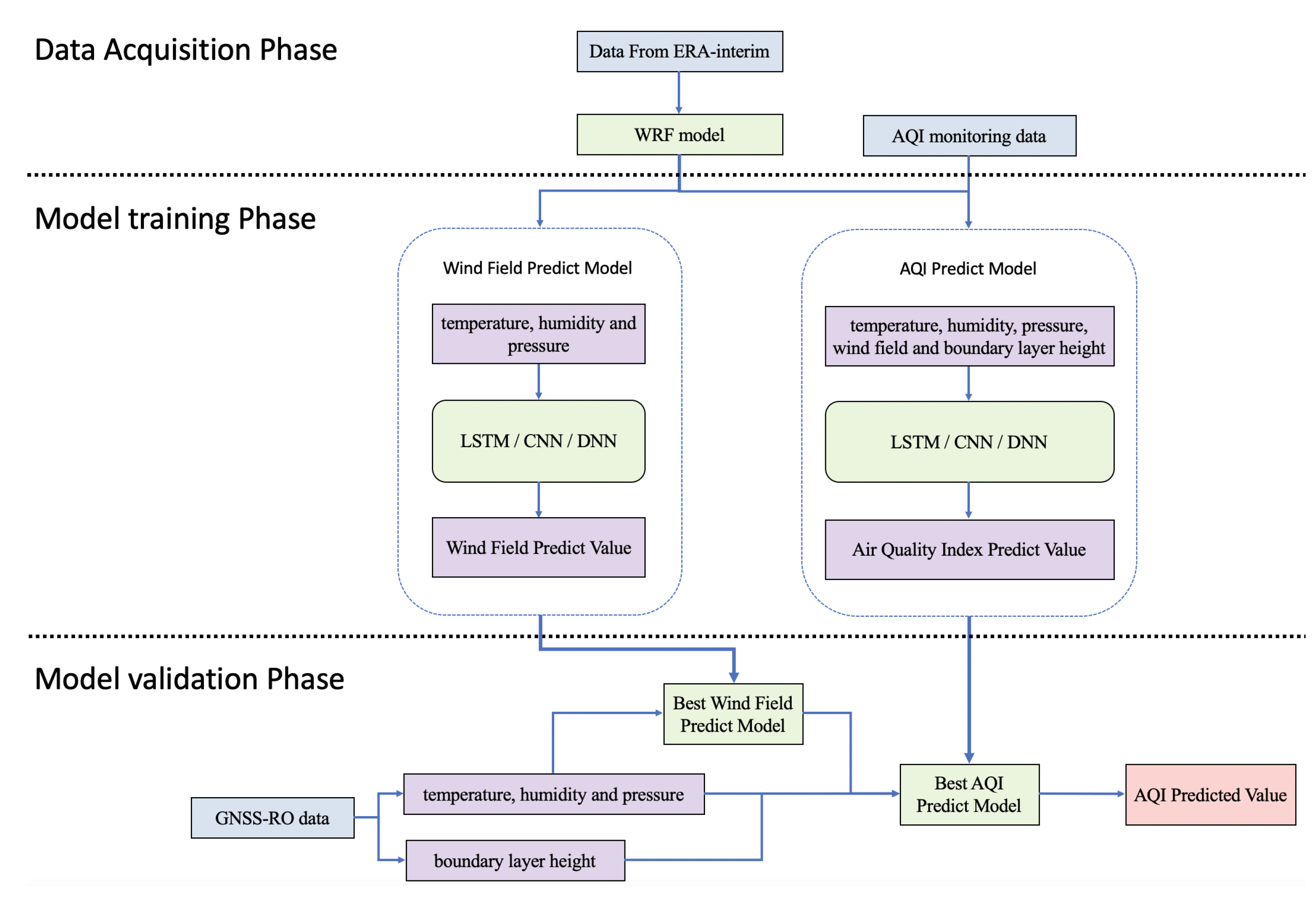
Figure 1. Overall workflow.
Atmosphere 14 00058 g001
Figure 2. Schematic diagram of the air quality index in the Beijing-Tianjin-Hebei region of China.
Atmosphere 14 00058 g002
Figure 3. LSTM air quality index prediction results.
Atmosphere 14 00058 g003
Figure 4. CNN air quality index prediction results.
Atmosphere 14 00058 g004
Figure 5. DNN air quality index prediction results.
Atmosphere 14 00058 g005
Figure 6. Air quality index prediction errors of different neural network models.
Atmosphere 14 00058 g006
Figure 7. Comparison of predicted and observed AQI values in LSTM.
Atmosphere 14 00058 g007
Figure 8. Comparison of different ratios of the training set and test set.
Atmosphere 14 00058 g008
Figure 9. Importance of different features in the model.
Atmosphere 14 00058 g009
Figure 10. Effect of different learning rates on model prediction effectiveness.
Atmosphere 14 00058 g010
Figure 11. Effect of different epoches on model prediction effectiveness.
Atmosphere 14 00058 g011
Table 1. Ablation test result.
rRMSEMAE
Baseline2.6680%8.952
+ wind field2.5009%8.865
+ boundary layer height2.5137%8.769
+ wind field and boundary layer height2.3948%8.553
Table 2. Training time and prediction time for different models.
LSTMCNNDNNWRF
Train Time1 min 42 s1 min 2 s31 s0 s
Predict Time0.46 s0.47 s0.48 s15 min 32 s
Relative Pred Time0.049%0.050%100%0.052%
Disclaimer/Publisher’s Note: The statements, opinions and data contained in all publications are solely those of the individual author(s) and contributor(s) and not of MDPI and/or the editor(s). MDPI and/or the editor(s) disclaim responsibility for any injury to people or property resulting from any ideas, methods, instructions or products referred to in the content.