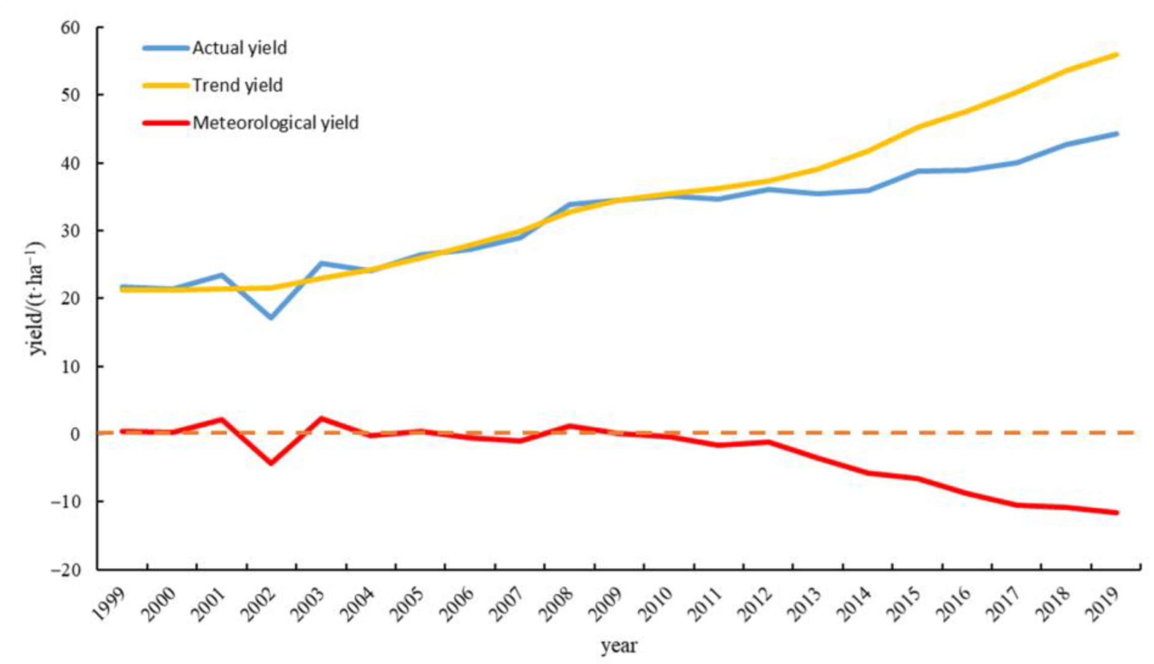
3.2. Screening of Key Meteorological Factors
The KMO statistic test is required before a principal component analysis is used, and the KMO statistic was 0.422 < 0.600, which is not suitable for variable importance ranking using a principal component analysis [
52]. In previous studies by Li et al. [
10] and Shen et al. [
53], GRA was utilized to screen key meteorological factors. The data of Yantai City from 1999 to 2019 were standardized, and the GRA was used to calculate each index’s correlation coefficients in the sub-sequence and the parent sequence. Combined with Equation (4), the average value of the correlation coefficient of each meteorological factor was taken as the grey relational coefficient between each meteorological factor and the meteorological yield.
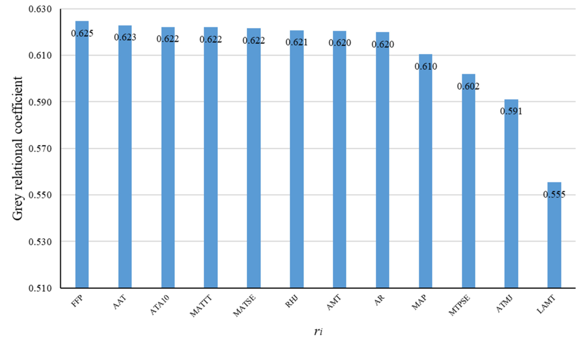
GRA was conducted on twelve meteorological factors and meteorological yield to obtain the grey correlation coefficient. The results are shown in
Figure 3.
The correlation degree of different meteorological factors was sorted, and the ranking order represents the impact degree of different meteorological factors on apple meteorological yield.
Figure 3 illustrates that the twelve meteorological factors affecting apple meteorological yield were sorted as follows: the frost-free period, the annual mean temperature, the accumulated temperature above 10 °C, the March–October mean temperature, the June–August mean temperature, the July relative humidity, the annual extreme low temperature, the annual difference in temperature, the annual average precipitation, the June–August precipitation, the mid-January mean temperature, and the coldest month mean temperature.
Grey correlation analysis can be employed to obtain the correlation ranking among variables, but it is not easy to judge the promoting or inhibiting relationship between variables. Therefore, key factors are initially screened by a grey relational analysis. Generally, two to four variables are selected as key variables [
54,
55]. The low threshold is set by selecting eight variables as candidates for key meteorological factors based on the initial screening. Thus, the meteorological factors with a correlation coefficient greater than 0.62 are defined as the key meteorological factors. The preliminary screening results include the frost-free period, the annual mean temperature, the accumulated temperature above 10 °C, the March–October mean temperature, the June–August mean temperature, the July relative humidity, the annual extreme low temperature, and the annual difference in temperature. Producers should pay more attention to the changes in the key meteorological factors, timely adjust the field’s microclimate, and formulate a reasonable fruit-tree management plan to prevent the dramatic decline of apple yield.
3.3. Construction of Meteorological Yield Forecast Model
SPSS 28.0 was applied for the collinearity test, principal component analysis, and multiple linear regression. The correlation and scatter diagrams were conducted with R version 4.2.2 using the packages dplyr, tidyverse, and ggplot2 for visualization of data in plots and heatmaps [
56,
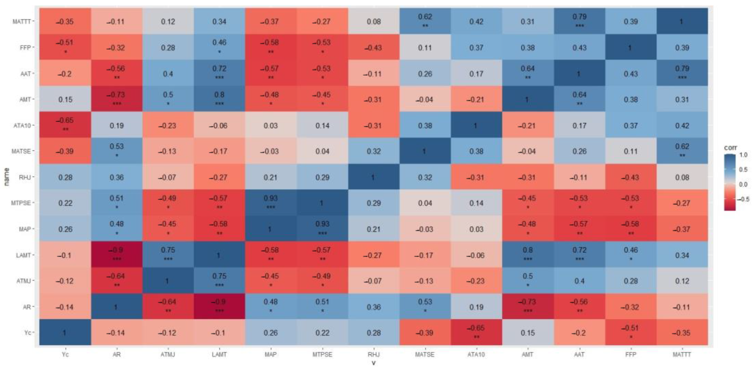
57]. The results of the correlation analysis are shown in
Figure 4.
Figure 4 demonstrates that, under the two-tailed test conditions, the meteorological yield was significantly correlated with the frost-free period and the accumulated temperature above 10 °C. Additionally, the accumulated temperature above 10 °C had an extremely significant inhibitory effect on the meteorological yield of apples (
p < 0.01), and the frost-free period had a significant inhibitory effect on the meteorological yield of apples (
p < 0.05). There were certain correlations among different meteorological factors. For example, the annual mean temperature was extremely significantly positively correlated with the March–October mean temperature, the annual extreme low temperature, and the coldest month mean temperature (
p < 0.01), while the annual mean temperature was extremely significantly negatively correlated with the annual difference in temperature and the annual average precipitation (
p < 0.01). The annual difference in temperature was extremely significantly negatively correlated with the coldest month mean temperature, the mid-January mean temperature, the annual mean temperature, and the annual extreme low temperature (
p < 0.01), while the annual difference in temperature was significantly positive correlated with the annual average precipitation, the June–August precipitation, and the June–August mean temperature (
p < 0.05). The coldest month mean temperature was extremely significantly positively correlated with the mid-January mean temperature, the annual mean temperature, and the annual extreme low temperature (
p < 0.001). The correlation analysis shows that the correlation between meteorological factors was strong, but the correlation between meteorological factors and meteorological yield was not high. The multiple regression equation and variance analysis are shown in Equation (17) and
Table 2.
It can be remarked from the results of variance analysis in
Table 2 that Significance F value is greater than 0.05, which indicates that the multiple regression equation was not significant and could not be used for prediction. This phenomenon is probably caused by the serious collinearity between meteorological factors. Therefore, the collinearity diagnosis of meteorological factors needs to be checked. The collinearity diagnosis result is shown in
Table 3.
Table 3 shows the
values of different meteorological factors were greater than 10, and the
values of the annual difference in temperature indicators were far more than 100, indicating that there is serious multicollinearity among different meteorological factors in Yantai. The meteorological factors in the meteorological system will interact and influence each other, so that one meteorological factor can be calculated from other meteorological factors. For example, the annual difference in temperature is obtained by subtracting the mean temperature of the coldest month from the mean temperature of the hottest month in a year. Interaction may be the reason for the serious collinearity of meteorological factors in Yantai City. The direct establishment of regression models will cause serious information coverage problems making the original data unable to be fully utilized. Because of the serious collinearity between meteorological factors in Yantai City, the established multiple regression model is invalid. A principal component analysis reduces the dimensionality of multivariate factors, extracts most of the information of the original data, and reduces the coverage between the information. Therefore, a principal component analysis can solve the problem.
The principal component analysis model was established, and the Bartlett sphericity test was performed on the standardized correlation coefficient matrix. The significance was 0.00 < 0.05; thus, the original hypothesis of Bartlett’s sphericity test was rejected, and the principal component analysis could be performed. The meteorological yield and twelve meteorological factors were analyzed using a principal component analysis. The results are shown in
Table 4.
Table 4 demonstrates that the cumulative contribution of the first five principal components reached 90.076%, which meets the requirement of a cumulative contribution of >85% for a principal component analysis. It indicates that most of the information in the original data has been extracted at this point. For its principal components, only five principal components were needed to represent the twelve indicators, and the contribution of each variable to the principal components constitutes the principal component matrix, as shown in
Table 5.
As shown in
Table 5, the principal component
is composed of the annual mean temperature, the annual difference in temperature, the coldest month mean temperature, and the annual extreme low temperature. The principal component
is composed of the June–August mean temperature, the March–October mean temperature, and the accumulated temperature above 10 °C. The principal component
is composed of the July relative humidity. The principal component
is composed of the annual average precipitation and the June–August precipitation. The principal component
is composed of the mid-January mean temperature. The principal components
can be named as temperature factor, growing season heat factor, humidity factor, precipitation factor, and cooling factor, respectively. The principal component
can be expressed as:
The principal components
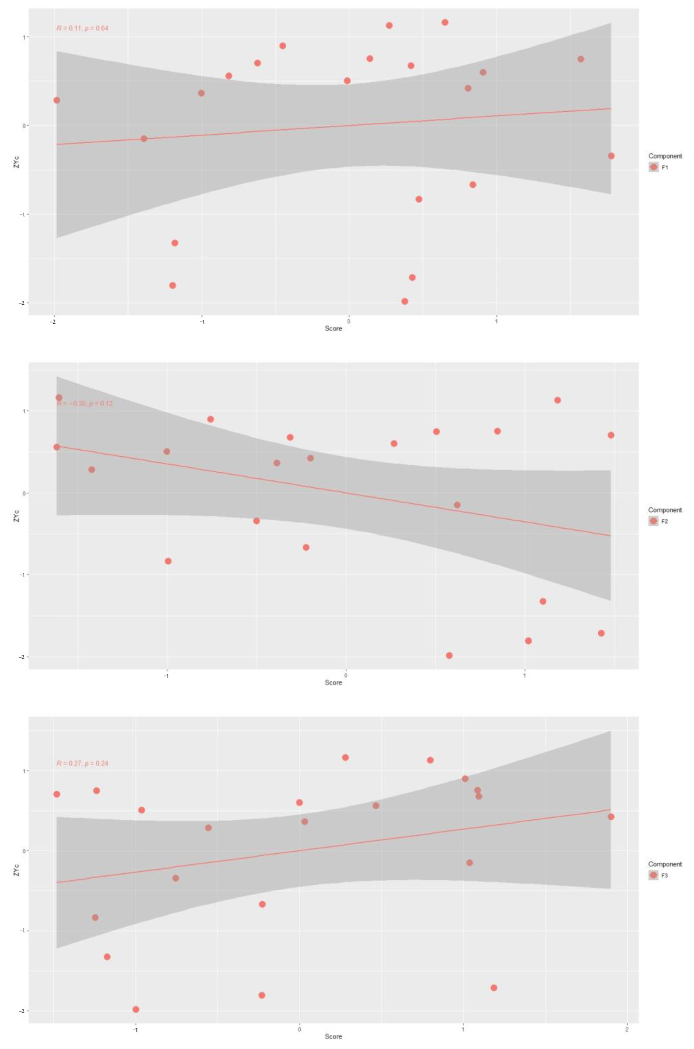
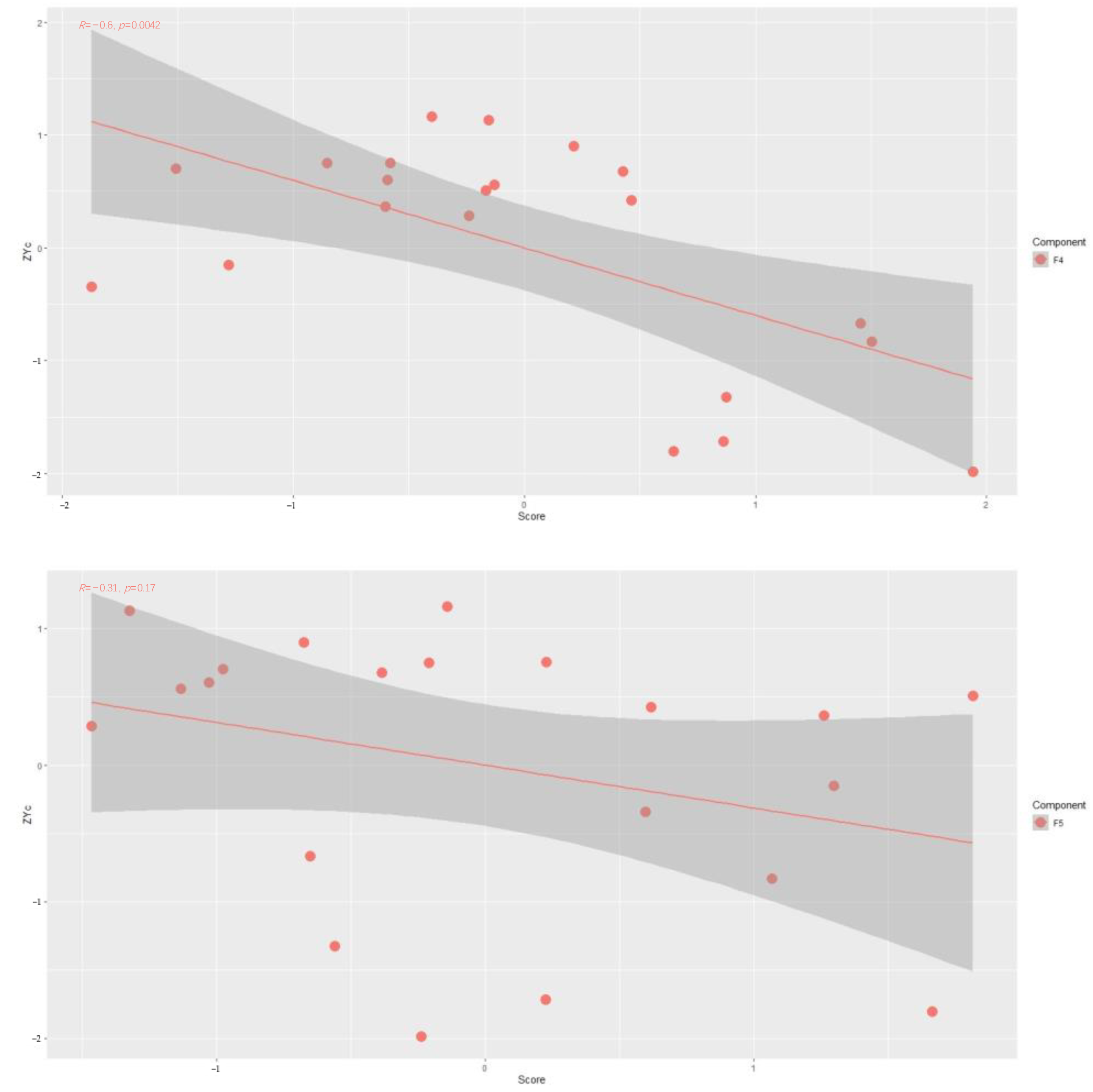
were taken as independent variables, and the method of multiple linear regression was adopted to perform an ordinary least squares (OLS) analysis on meteorological yield after the normalization of dependent variables. The relationships between principal components
and normalized meteorological yield are shown in
Figure 5.
Figure 5 demonstrates that with the increase of the independent variables
and
, the value of
increases continuously;
, and
with the opposite trend of change, indicating that
and
have a negative correlation coefficient, and
has a positive correlation coefficient with
and
.
According to the standardized residual analysis (
Figure 6), the standardized residual follows the mean value of −1.73 × 10
−16 and the normal distribution with a standard deviation of 0.894, which can be approximated following a normal distribution with a mean of zero and a standard deviation of one. The residual distribution satisfies the applicable range of multiple linear regression. Meanwhile, the value of the Durbin–Watson statistic is closer to two and there is less correlation between the residual terms. The value of the Durbin–Watson statistic of the model constructed in this paper is 1.658, which indicates that the residual terms are not correlated.
According to the above analysis, the relationship between the dependent variable
and the independent variables
is linear. The independent variables
are not random. Moreover, there is no exact linear relationship between two or more independent variables due to the extraction of the PCA. The expected value of the residual in terms of the independent variable is 0:
. The variance of the residual term is the same for all observations:
. The residual term is not correlated between the observed values:
. The residual term is normally distributed. All the basic assumptions of the multiple linear regression model are consistent. Therefore, the MLR–PCA was established and the backward stepwise regression analysis results are shown in
Table 6.
Table 6 shows that the
values of meteorological yield after the normalization of the principal components
and the dependent variable are all less than 10, indicating that the principal component analysis solved the interference of multicollinearity on the prediction model. The principal components
, and
are negatively correlated with the meteorological yield, which means the higher the growing season heat factor, precipitation factor, and cooling factor are, the lower the meteorological yield is. The principal components
and
are positively correlated with meteorological yield, which means that the higher temperature factor and humidity factor are, the higher the meteorological yield is. The regression coefficient is consistent with the results observed in
Figure 5. The expression of multiple linear regression is:
According to Equations (18) and (19), the standardized linear equation can be expressed as:
According to Equation (20), the coefficients of the accumulated temperature above 10 °C, the June–August precipitation, the annual average precipitation, the June–August mean temperature, and the March–October mean temperature were large. Combined with the conclusion in
Section 3.2 “Screening of Key Meteorological Factors”, the key meteorological factors were the accumulated temperatures above 10 °C, the March–October mean temperature, and the June–August mean temperature.
The standardized linear equation was destandardized and the expression of the linear equation was obtained as:
Using Equation (19), in terms of the temperature factor, the whole period of the increase of the temperature factor on apple meteorological yield does not have a significantly positive effect. This result proves that there is not a simple linear relationship between the temperature factor and the meteorological yield in Yantai, but there may be a complex nonlinear interaction. In terms of the growing season heat factor, there is a significantly negative correlation (p < 0.05) between the growing season heat factor and apple’s meteorological yield. This result proves that the heat supply in the growing period of Yantai may exceed the heat required for the development of apples. High temperatures can easily cause thermal damage, resulting in cell dehydration, affecting the physiological metabolic activities of plants and reducing the yield. In terms of the humidity factor, there is a positive correlation (p < 0.1) between the humidity factor and apple’s meteorological yield. This shows that Yantai summer humidity may not meet the needs of apple growth. In summer, when the humidity is low and the temperature is high, the stomata on the leaves of plants will close to keep the water in the plant. The closure of stomata will make the leaves unable to capture carbon dioxide, leading to starvation. In terms of precipitation factor, the precipitation factor on apple meteorological yield over the whole period has an extremely significantly negative effect (p < 0.001). This means that the precipitation in Yantai exceeds the amount needed for apple growth. Excessive precipitation may cause waterlogging, and the surge in soil water content may cause anoxia, which will cause a series of hazards. In terms of cooling factor, the cooling factor on apple meteorological yield over the whole period has an extremely significantly negative effect (p < 0.01). The result indicates that low value of cooling, especially in winter, significantly reduces apple’s yield. When apple trees cannot meet the cooling requirements for releasing dormancy, forcibly breaking dormancy will greatly reduce their flowering and fruit setting rates and affect the apple yield.
3.4. Establishment and Evaluation of Comparative Models for Forecasting Meteorological Yield
Lasso regression avoids the distortion of the regression results caused by multicollinearity and endogeneity between variables in the regression process by rapidly compressing the coefficients of nonimportant explanatory variables to zero. We chose to compare the fitting effect and prediction results of lasso regression and the MLR–PCA model constructed in this paper and evaluate whether the prediction accuracy was improved by the MLR–PCA model. Lasso regression was conducted with R version 4.2.2 using the packages glmnet for visualization of data (
Figure 7).
The lambda for which we choose to cross-validate the model with the smallest mean error is denoted as lambda.min. According to
Figure 7b, the value of lambda.min is 1.00, and the corresponding number of important explanatory variables is 3. Combining with
Figure 7a, the important explanatory variables were the frost-free period, the accumulated temperature above 10 °C, and the June–August mean temperature. In order to compare the fitting effect and significance of the model [
58], the multiple linear regression model was established with important explanatory variables as independent variables and meteorological yield as dependent variables.
The goodness-of-fit and significance of the two models were compared, including MLR–PCA and lasso regression. The results are shown in
Table 7. It can be seen from
Table 7 that the regression effect of the MLR–PCA model and the lasso regression model is extremely significant (
p < 0.01). In addition, the goodness-of-fit of MLR–PCA is higher than that of the lasso regression model.
In order to verify whether MLR–PCA analysis can effectively improve the model accuracy, the relevant data from Yantai City in 2020 were used [
40], the meteorological yield forecasts of apple from the MLR–PCA model and the lasso regression model were calculated and combined with the harmonic weight trend yield forecast method [
48,
49,
50]. The predicted value of apple yield was obtained, and the yield prediction effects of the three models are shown in
Table 8.
By comparing the methods, the predicted value of the MLR–PCA model was 47.256 t·ha−1, compared with the actual yield of 44.128 t·ha−1. The relative error was 7.089%, which was the smallest among the selected models, indicating that the MLR–PCA model is superior and accurate in forecasting.

